Roles of climate variability on the rapid increases of early winter haze pollution in North China after 2010

North China experiences severe haze pollution in early winter, resulting in many premature deaths and considerable economic losses. The number of haze days in early winter (December and January) in North China (HD_NC) increased rapidly after 2010 but declined slowly before 2010, reflecting a trend reversal. Global warming and emissions were two fundamental drivers of the long-term increasing trend of haze, but no studies have focused on this trend reversal. The autumn sea surface temperature (SST) in the Pacific and Atlantic, Eurasian snow cover and central Siberian soil moisture, which exhibited completely opposite trends before and after 2010, might have close relationships with identical trends of meteorological conditions related to haze pollution in North China. Numerical experiments with a fixed emission level confirmed the physical relationships between the climate drivers and HD_NC during both decreasing and increasing periods. These external drivers induced a larger decreasing trend of HD_NC than the observations, and combined with the persistently increasing trend of anthropogenic emissions, resulted in a realistic, slowly decreasing trend. However, after 2010, the increasing trends driven by these climate divers and human emissions jointly led to a rapid increase in HD_NC.

1 Introduction

Haze pollution, characterized by low visibility and a high concentration of fine particulate matter (PM_2.5), has become a serious environmental and social problem in China, as haze dramatically endangers human health, ecological sustainability and economic development (Ding and Liu, 2014; Wang and Chen, 2016). Exposure to PM_2.5 was estimated to cause 4.2 million premature deaths worldwide in 2015 (Cohen et al., 2017), and PM_2.5 caused up to 0.96 million premature mortalities in China in 2017 (Lu et al., 2019). Air pollution accounts for a loss of 1.2 %–3.8 % of the gross national product (GNP) annually (Zhang and Crooks, 2012). The most polluted areas in China are North China (NC; 34–42 ^∘ N, 114–120^∘ E), the Fenwei Plain, the Sichuan Basin and the Yangtze River Delta; among them, NC is the most polluted (Yin et al., 2015). Meteorological conditions characterized by low surface wind speeds and a shallow boundary layer result in stagnant air, which limits the horizontal and vertical dispersion of particles and induces the accumulation of pollutants (Niu et al., 2010; Wu et al., 2017; Shi et al., 2019). High relative humidity favors the hygroscopic growth of pollutants (Ding and Liu, 2014; Yin et al., 2015), and anomalous ascending motions weaken the downward invasion of cold and clear air from high altitudes (Zhong et al., 2019). The forecasting of meteorological conditions is more accurate on the synoptic scale, but the predictions of interannual variations are not good enough. Thus, the prediction of haze is a considerable challenge.

Previous studies have proven that the interannual to decadal variations in winter haze have strong responses to external forcing factors, such as the sea surface temperature (SST) in the Pacific and Atlantic, snow cover and soil moisture (Xiao et al., 2015; Yin and Wang, 2016a, b; Zou et al., 2017). Anomalies of these factors exerted their impacts to modulate local dispersion conditions by atmospheric teleconnections and greatly intensified haze pollution in NC. The eastern Atlantic/western Russia (EA/WR), western Pacific (WP) and Eurasian (EU) patterns served as effective atmospheric bridges linking distant and preceding external factors to the anomalous anticyclonic circulations over northeastern Asia (Yin and Wang, 2017; Yin et al., 2017). With enhanced anticyclonic anomalies, the haze pollution in NC was significantly aggravated by poor ventilation conditions and high moisture.

The long-term trend of haze pollution has always been attributed to increasing human activities directly related to aerosol emissions (Yang et al., 2016; Li et al., 2018). It is true that emissions are important in the formation of haze, but their role varies from region to region (Mao et al., 2019). The trend of haze days in Yangtze River Delta and Pearl River Delta was closely related to the trend of particle emissions (Fig. S1b, c), whereas a weak correlation existed in Fenwei Plain (Fig. S1d). A surprising phenomenon can be seen in NC: the number of winter haze days and particle emissions showed similar trends before the early 1990s, but their close relationship disappeared afterward (Fig. S1a). Many recent studies have also shown that the long-term trend in the haze problem has likely been driven by global warming (Horton et al, 2014; Cai et al., 2017). Weakening surface winds have been reported over land over the last few decades, while the global surface air temperature (SAT) has warmed significantly (Mcvicar et al., 2012). In addition, enhanced vertical stability, which favors the accumulation of pollutants, has been observed with global warming (Liu et al., 2013). However, none of the abovementioned studies focused on the change in the haze trend. Over the past few decades, the global and Northern hemispheric SAT averages have generally displayed a continuous warming trend, which was not exactly similar to the trend of haze days in NC (Fig. S2). It follows that haze pollution, especially the change in its trend, is regulated by multiple drivers and that the long-term impacts of external forcing factors, which efficiently modulate the interannual and decadal variations in haze, deserve further investigation.

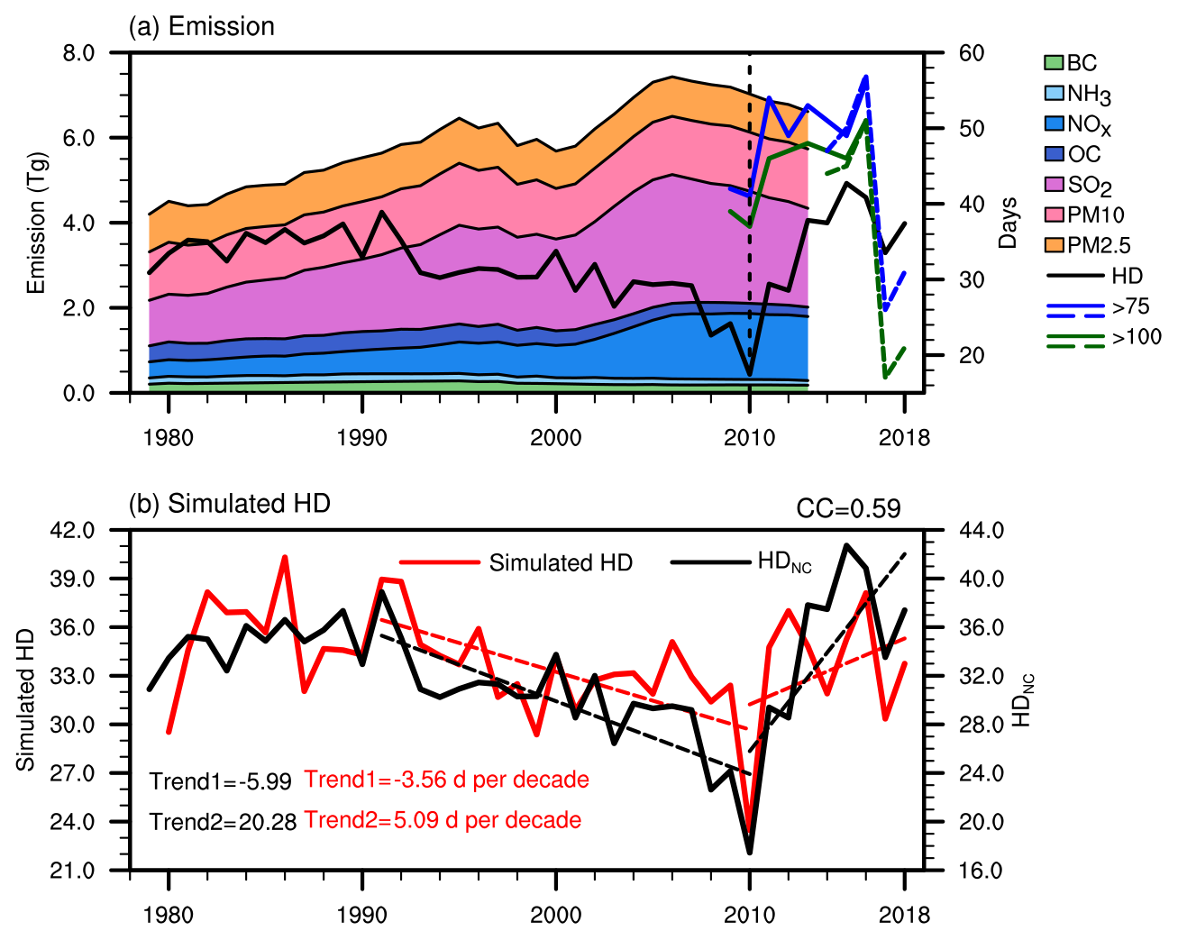
Figure 1 (a) Variations in the December and January emissions (unit: Tg) of black carbon (BC), ammonia (NH₃), nitrogen oxide (NO_x), organic carbon (OC), sulfur dioxide (SO₂), PM₁₀ and PM_2.5 over North China from 1979 to 2013 and the variation in HD_NC from 1979 to 2018 (black solid line). The blue and green solid (dashed) lines indicate the number of days when the hourly PM_2.5 concentrations exceeded 75 and 100 µg m⁻³, respectively, from 2009 to 2016 (2014 to 2018) using Beijing (North China) observed data from the US embassy (China National Environmental Monitoring Centre). (b) Temporal evolution of HD_NC (in black) and simulated haze days (unit: days; red) in NC. The dashed lines denote linear regressions for 1991–2010 (P1) and 2010–2018 (P2). Trend 1 and Trend 2 represent the linear trends of the observed (black) and simulated (red) haze days in P1 and P2, respectively.

2 Datasets and methods

2.1 Data description

Monthly mean meteorological data from 1979 to 2018 were obtained from NCEP/NCAR Reanalysis datasets ($\mathrm{2.5}{}^{\circ }\times \mathrm{2.5}{}^{\circ }$), including the geopotential height at 500 hPa (H500), vertical wind from the surface to 150 hPa, surface air temperature (SAT), wind speed and special humidity at the surface (Kalnay et al., 1996). The boundary layer height (BLH, $\mathrm{1}{}^{\circ }\times \mathrm{1}{}^{\circ }$) values were from ERA-Interim reanalysis data obtained from the European Centre for Medium-Range Weather Forecasts (ECMWF; Dee et al., 2011). The number of haze days was calculated from the long-term meteorological data, mainly based on observed visibility and relative humidity (Yin et al., 2017). The PM_2.5 concentrations from 2009 to 2016 were acquired from the US embassy, and the PM_2.5 concentrations from 2014 to 2018 were obtained from the China National Environmental Monitoring Centre. Monthly total emissions of BC, NH₃, NO_x, OC, SO₂, PM₁₀ and PM_2.5 were obtained from the Peking University emission inventory. The monthly mean extended reconstructed SST data ($\mathrm{2}{}^{\circ }\times \mathrm{2}{}^{\circ }$) were obtained from the National Oceanic and Atmospheric Administration (Smith et al., 2008). The monthly snow cover data were supplied by Rutgers University (Robinson et al., 1993). The monthly soil moisture data ($\mathrm{0.5}{}^{\circ }\times \mathrm{0.5}{}^{\circ }$) were downloaded from NOAA's Climate Prediction Center (Huug et al., 2003).

2.2 GEOS-Chem description and experimental design

We used the GEOS-Chem model to simulate PM_2.5 concentrations (http://acmg.seas.harvard.edu/geos/, last access: 22 October 2020). The GEOS-Chem model was driven by MERRA-2 assimilated meteorological data (Gelaro et al., 2017). The nested grid over Asia (11^∘ S–55^∘ N, 60–150^∘ E) had a horizontal resolution of 0.5^∘ latitude by 0.625^∘ longitude and 47 vertical layers up to 0.01 hPa. The GEOS-Chem model includes fully coupled O₃−NO_x–hydrocarbon and aerosol chemical mechanisms with more than 80 species and 300 reactions (Bey et al., 2001; Park et al., 2004). The PM_2.5 components simulated in GEOS-Chem include sulfate, nitrate, ammonium, black carbon and primary organic carbon, mineral dust, secondary organic aerosols and sea salt. The GEOS-Chem model has been widely used. Dang and Liao (2019) used the model to show that the simulated spatial patterns and daily variations of winter PM_2.5 based on GEOS-Chem agree well with the observations from 2013 to 2017, which are the available years with measured PM_2.5. We selected the year of 2015, as emission reduction just begun to strengthen, and 2017, as this is when the air pollution prevention and management plan for “2+26” cities launched (Yin and Zhang, 2020), as two representative years to simulate the actual PM_2.5 concentrations, so as to evaluate the performance of the GEOS-Chem model. The simulation results are very close to the observed data (Fig. S3), with high correlation coefficients reaching 0.88 and 0.85 in 2015 and 2017, respectively, indicating that this model could basically reflect the change in actual PM_2.5 concentrations.

In this study, we designed two kinds of experiments: one was an experiment for simulating PM_2.5, and the other was a composite using simulated data. The simulation had changing meteorological fields in winter from 1980 to 2018 and fixed emissions in 2010 representing a high emission level. The emission data in 2010 were from MIX 2010 (Li et al., 2017). The numerical experiment was performed to examine the variation in PM_2.5 in the meteorological parameters during the 1980–2018 period under fixed-emission scenarios.

The composite was conducted to analyze the differences in the simulated HD_NC according to the years selected for the external forcing factors. Using the simulated dataset with the fixed-emission scenario, we were capable of eliminating the impacts of emissions and simply considering the effect of the four external forcing factors. The 4 (2) years with the largest (favored years) and smallest (unfavored years) four external forcing indices (i.e., SST_P, $-\mathrm{1}\times {\mathrm{ST}}_A$, Snowc and $-\mathrm{1}\times \mathrm{Soilw}$) were selected, and the differences in the simulated HD_NC under these four conditions in P1, 1991–2010, (P2, 2010–2018) were calculated. The simulated HD_NC in favored years minus the simulated HD_NC in unfavored years was calculated to analyze the effect of these four forced factors.

2.3 Statistical methods

In this study, the statistical model of fitted HD_NC was built based on multiple linear regression (MLR). This approach, a model-driven method, was ultimately expressed as a linear combination of K predictors (x_i) that could generate the least error of prediction $\stackrel{\mathrm{̃}}{y}$ (Wilks, 2011). With coefficients β_i, intercept β₀ and residual ε, the MLR formula can be written in the following form: $\stackrel{\mathrm{̃}}{y}={\mathit{\beta }}_{\mathrm{0}}+\sum {\mathit{\beta }}_i{x}_i+\mathit{\epsilon }$.

The trends calculated in this study were obtained by linear regression after a 5 year running average. This method removed the interannual variation and more prominent trend characteristics. Moreover, the stage trends were calculated according to the inflection point, which passed the Mann–Kendall test.

3 Trend change in early winter haze

In winter in North China, the haze pollution early in the season is the most serious (Yin et al., 2019). The number of haze days in early winter (December and January) in North China (HD_NC) reached a remarkable inflection point in 2010 (Fig. 1a), passing the Mann–Kendall test. The trend of HD_NC was vastly different before and after 2010: it slowly decreased during the 1991–2010 period (P1) at a rate of 4.67 d per decade but rapidly increased after 2010 (P2, 2010–2018) at a rate of 25.43 d per decade, with both of these values passing the 95 % t test. Recent studies have generally revealed that, based on observations, the number of boreal winter haze days across NC had a slightly decreasing trend after 1990 (Ding and Liu, 2014; He et al., 2019; Mao et al., 2019; Shi et al., 2019), which is consistent with the decreasing trend presented by the dataset in our research. Excluding the year 2010 did not affect the change in the trend of the two periods, with a decreased rate of 3.82 d per decade during the 1991–2009 period and an increased rate of 20.76 d per decade during the 2011–2018 period (passing the 95 % t test). In addition, Dang and Liao (2019) confirmed the varying trend of HD_NC via simulations of the global 3-D chemical transport (GEOS-Chem) model; using the well-simulated frequency of serious haze days in winter, they also revealed the abovementioned changing trend of HD_NC, i.e., decreasing in the early period and increasing in the later period. To further determine the reliability of the post-2010 upward trend of HD_NC, we used hourly PM_2.5 concentrations observed at the US embassy in Beijing from 2009 to 2017 and the PM_2.5 concentrations over North China monitored by China National Environmental Monitoring Centre from 2014 to 2018 to count the number of days when the PM_2.5 concentrations were >75 and >100 µg m⁻³ (Fig. 1a). These statistics also reflected the rising trend after 2010 as well as the improved air quality in 2017 and a rebound in pollution in 2018. Although there was a certain gap between HD_NC (based on visibility and humidity) and these statistics, the two datasets revealed the same variations after 2010, and the statistics confirmed the robustness of the observed HD_NC.

The above analysis substantiated the rapid aggravation of haze pollution in early winter after 2010. With regard to the increase in air pollution, there is no doubt that anthropogenic emissions were the fundamental cause of this long-term variation. Before the mid-2000s, the particle emissions throughout NC sustained stable growth but gradually began to decline afterward, which is inconsistent with the trend of HD_NC or even contrary in some subperiods. The previous decreasing trend of HD_NC hid the effects of the increased pollutant emissions; thus, people ignored the pollution problem and failed to control it in time. As a consequence, the subsequent rise in HD_NC was extremely rapid and seriously harmed the biological environment and human health. The stark discrepancy between the trends of pollutant emissions and HD_NC strongly indicate that anthropogenic emissions were not the only factor leading to a sharp deterioration in air quality after 2010 (Wei et al., 2017; Wang, 2018). Therefore, an important question must be asked: in addition to human activities, what factors caused the rapidly increasing trend of HD_NC after 2010?

As mentioned above, local meteorological factors could modulate the capacity to disperse and the formation of haze particles, which have critical influences on the occurrence of severe haze pollution. To reveal the impacts of meteorological conditions on the changing trend of HD_NC, the area-averaged linear trends of these meteorological factors in NC during P1 and P2 were calculated – all of which exceeded the 95 % confidence level (Fig. 2). In P1, the area-averaged linear trends of the boundary layer height (BLH), wind speed and omega all showed significant positive trends, while specific humidity showed a significant negative trend in NC; these conditions favored a superior air quality (Niu et al., 2010; Ding and Liu, 2014; Yin et al., 2017; Shi et al., 2019; Zhong et al., 2019). However, the trends of these four meteorological factors completely reversed in P2. Reductions in the BLH and wind speed, the enhancement of moisture and an anomalous ascending motion resisted the vertical and horizontal dispersions of particles and helped more pollutants gather in relatively narrow spaces. These four meteorological factors expressed an evident influence on the change trend of HD_NC and showed reversed trends between P1 and P2, similar to HD_NC. Furthermore, the magnitudes of the change rates of these factors were stronger in P2 than in P1 (Fig. 2), and HD_NC displayed this feature as well. The GEOS-Chem simulations with changing emissions and fixed meteorological conditions failed to reproduce the change trend of haze (Dang and Liao, 2019); however, with varying meteorology and fixed emissions, they could recognize the interannual variation in haze days. We designed an experiment driven by changing meteorological conditions in winter from 1980 to 2018 and fixed emissions at the relatively high 2010 level. According to the technical regulation of the ambient air quality index (Ministry of Ecology and Environment of the People's Republic of China, 2012), a haze day was defined as a day with a daily mean PM_2.5 concentration exceeding 75 µg m⁻³. The simulations of the frequency of haze days in NC by GEOS-Chem reproduced the trend reversal of haze pollution (Fig. 1b). The simulation results were highly correlated with HD_NC and showed that the trend in P2 was stronger than that in P1, indicating that meteorological conditions drove the trend change in haze pollution.

4 Climate variability drove the trend reversal

According to many previous studies, the variabilities of the Pacific SST, Atlantic SST, Eurasian snow cover and Asian soil moisture play key roles in the interannual variations in haze pollution in NC (Xiao et al., 2015; Yin and Wang, 2016a, b; Zou et al., 2017), and the associated physical mechanisms have been evidently revealed. Thus, the following question is raised here: did these four factors drive the trend reversal of HD_NC, and if so, how?

As shown in Figure S4a, the preceding autumn SST in the Pacific, associated with the detrended HD_NC, presented a “triple pattern”, similar to a Pacific Decadal Oscillation (PDO), with two significant positive regions and one nonsignificant negative region (Yin and Wang, 2016a; Zhao et al., 2016). In the following research, the SST anomalies in the two positively correlated regions located in the Gulf of Alaska (40–60^∘ N, 125–165^∘ W) and the central eastern Pacific (5–25^∘ N, 160^∘ E–110^∘ W) were used to represent the effects originating from the North Pacific. The area-averaged September–November SST of these two regions was calculated as the SST_P index, and the correlation coefficients with HD_NC were 0.59 and 0.67 before and after removing the linear trend during the 1979–2018 period, respectively; both correlation coefficients were above the 99 % confidence level. The responses of the atmosphere to these positive SST_P anomalies were the positive phase of the EA/WR pattern and the enhanced anomalous anticyclone center over NC (Yin et al., 2017; Fig. S5). Modulating by such large-scale atmospheric anomalies, increased moisture, anomalous upward motion and reduced BLH and wind speed (Fig. S5) created a favorable environment for the accumulation of fine particles (Niu et al., 2010; Ding and Liu, 2014; Shi et al., 2019; Zhong et al., 2019). A numerical experiment based on the Community Atmosphere Model version 5 (CAM5) effectively reproduced the observed enhanced anticyclonic anomalies over Mongolia and North China in response to positive PDO forcing, which resulted in an increase in the number of wintertime haze days over central eastern China (Zhao et al., 2016). The trend changes in the North Pacific SST were examined in P1 and P2. Consistent with the changing trend of HD_NC, reversed trends were also found in the North Pacific, i.e., a significant negative trend during P1 and a positive trend during P2 over the two Pacific areas (Fig. 3a, b). These similar trend changes suggest that the North Pacific SST might have been a major driver of the abrupt change in HD_NC. It is clear that SST_P underwent a significant trend change around 2010 (Fig. 4a). Thus, the persistent decline in SST_Pduring P1 (at a significant rate of −0.2 ^∘C per decade, passing the 95 % t test; Table 1) contributed to the slowly decreasing trend of HD_NC (Fig. 4a) via the modulations of SST_P on the atmospheric circulation (Fig. S5). During P2, the larger increase in SST_P at a rate of 2.0 ^∘C per decade (passing 95 % t test) dramatically drove the rapid increase in HD_NC.

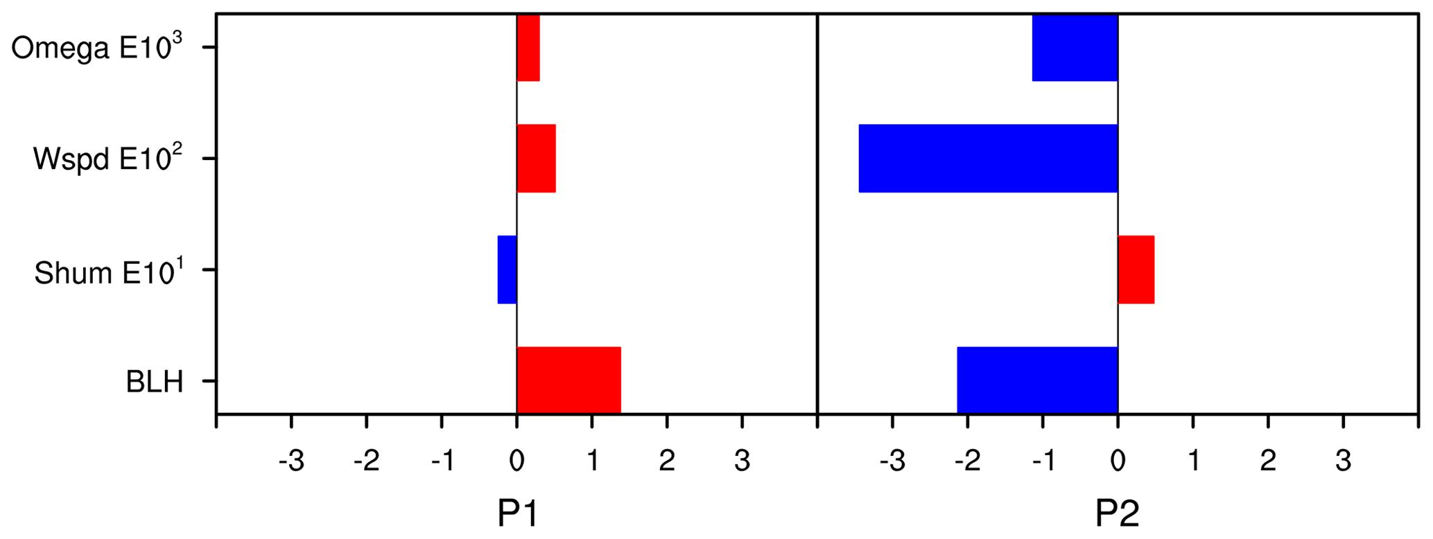
Figure 2 Area-averaged linear trends of the BLH (unit: m yr⁻¹), specific humidity (unit: % 10 yr⁻¹), surface wind speed (unit: m s⁻¹ 10² yr⁻¹) and omega (unit: pascals s⁻¹ 10³ yr⁻¹) over NC in early winter for the 1991–2010 (P1) and 2010–2018 (P2) periods. All datasets were 5-year running averages before calculating the trends.

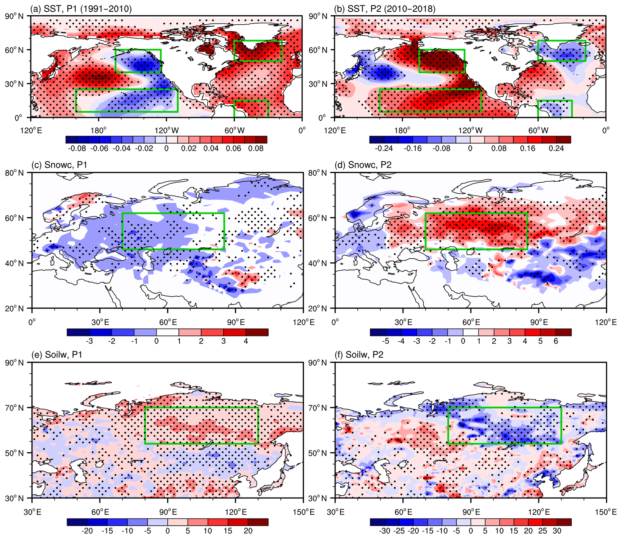
Figure 3 Linear trends of the Pacific and Atlantic SST (unit: ^∘C yr⁻¹; a, b), Eurasian snow cover (unit: % yr⁻¹; c, d) and central Siberian soil moisture (unit: mm yr⁻¹; e, f) for the 1991–2010 (P1) and 2010–2018 (P2) periods. All datasets were 5-year running averages before calculating the trends. The green boxes represent the regions where the four indices are defined. Black dots indicate that the trends were above the 95% confidence level.

Table 1 Correlation coefficients (CCs) between HD_NC and the SST_P, SST_A, Snowc and Soilw indices after detrending, and the trends of the SST_P, SST_A, Snowc and Soilw indices for the 1991–2010 and 2010–2018 periods. CC₁, CC₂ and CC₃ represent the correlation coefficients from 1979 to 2018, 1979 to 2010 and 2010 to 2018, respectively. “${}^{***}$” indicates that the CC was above the 99 % confidence level, “${}^{**}$” indicates that the CC was above the 95 % confidence level and “^*” indicates that the CC was above the 90 % confidence level.

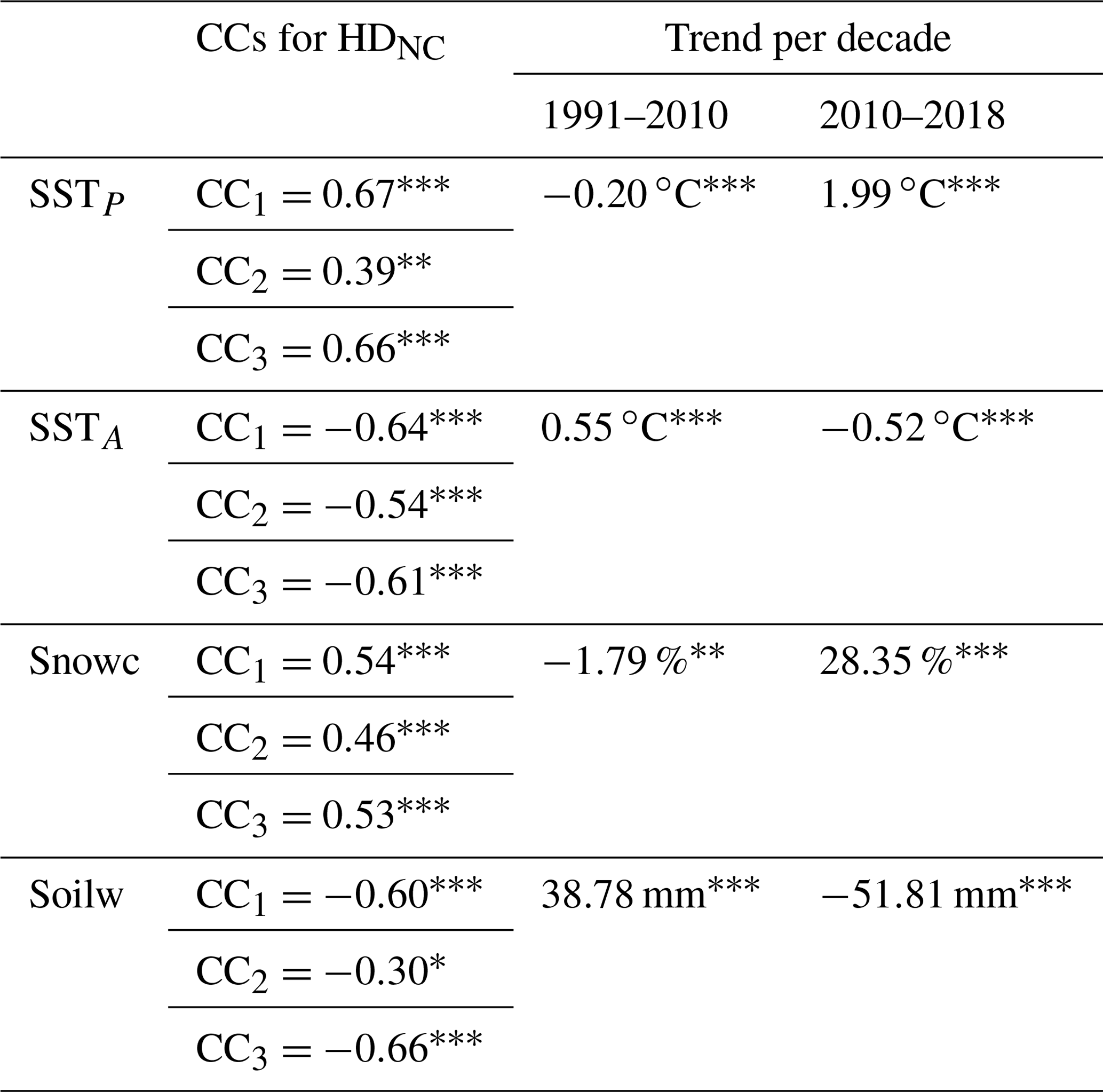
Besides the triple pattern in the Pacific, two areas exhibiting significant negative correlations with HD_NC were examined in the Atlantic (Shi et al., 2015): one located over southern Greenland (50–68^∘ N, 18–60^∘ W) and another located over the equatorial Atlantic (0–15^∘ N, 30–60^∘ W; Fig. S4a). The area-averaged September–November SST of the two negatively correlated regions in Atlantic was defined as the SST_A index, whose correlation coefficients with HD_NC were −0.55 and −0.64 from 1979 to 2018 before and after detrending, respectively (above the 99 % confidence level). The response of atmospheric circulation to these negative SST_A anomalies culminated in a positive EA/WR pattern, and the stimulated easterly weakened the intensity of East Asian jet stream (EAJS) in the high troposphere (Fig. S6). Influenced by the colder SST_A, there was a very obvious abnormal upward movement above the boundary layer, reducing both the BLH and the surface wind speed; thus, pollutants were prone to gather, causing haze pollution (Niu et al., 2010; Wu et al., 2017; Shi et al., 2019). With a linear barotropic model, Chen et al. (2019) confirmed the important role of subtropical northeastern Atlantic SST anomalies in contributing to the anomalous anticyclone over northeastern Asia and anomalous southerly winds over NC, which enhanced the accumulation of pollutants. The spatial linear trend in the SST of both Atlantic areas changed from positive in P1 to negative in P2, which was completely contrary to the trend of HD_NC (Fig. 3a, b). The SST_A reached an inflection point in 2010 (Fig. 4b) and contributed to the decrease in HD_NC during P1 (change rate of SST_A of 0.55^∘C per decade, passing the 95 % t test) and the increase in HD_NC during P2 (change rate of SST_A of −0.52^∘C per decade, passing the 95 % t test).

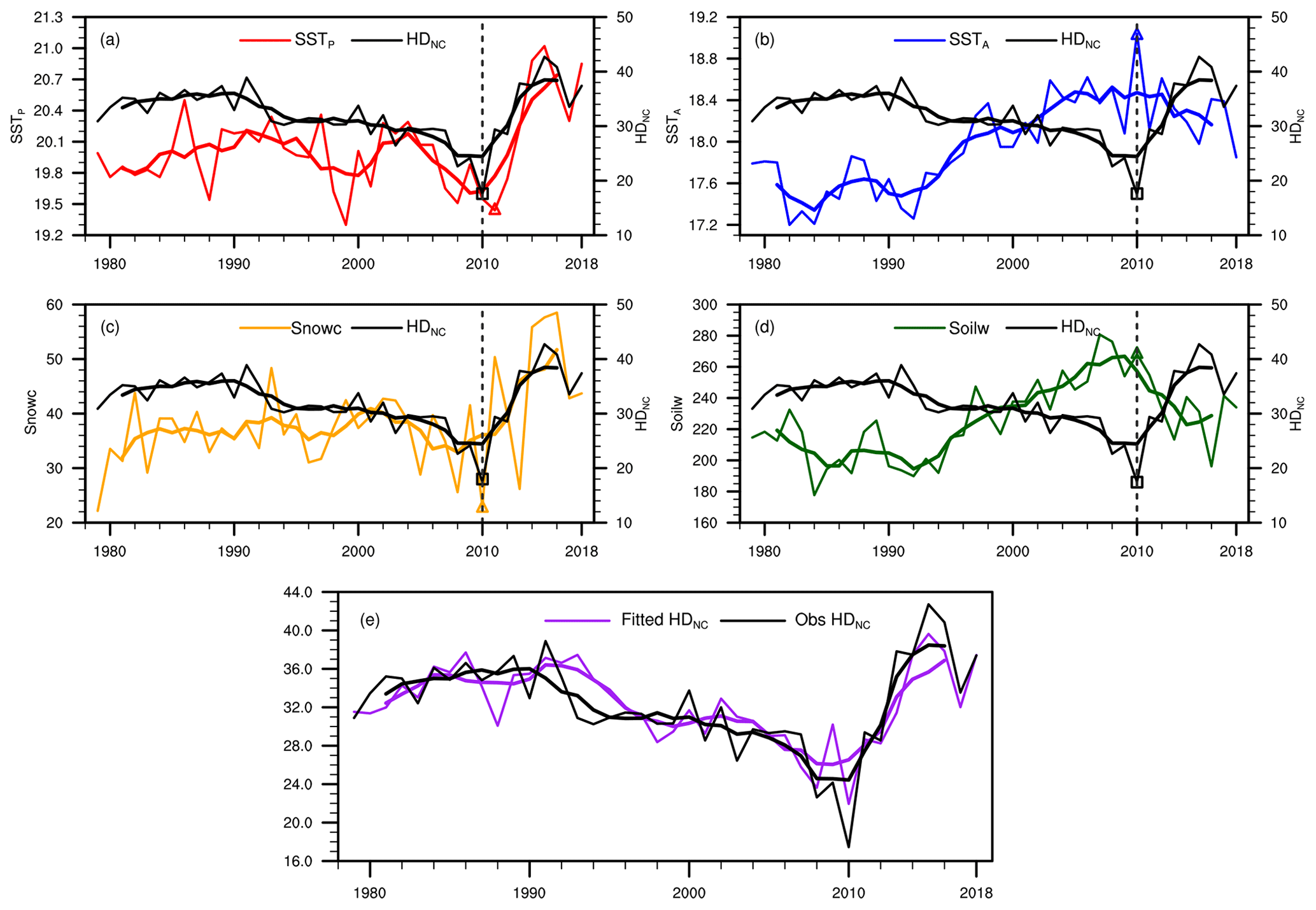
Figure 4 Variations in HD_NC (in black) and the SST_P (unit: ^∘C; a, red), SST_A (unit: ^∘C; b, blue), Snowc (unit: %; c, yellow) and Soilw (unit: mm; d, green) indices as well as the HD_NC values fitted by the MLR model for the above four factors (unit: days; e, purple) from 1979 to 2018. Thick lines indicate 5-year running averaged time series. The rectangles and triangles indicate the inflection points of HD_NC and the four indices, which were tested by the Mann–Kendall test.

The effect of Eurasian snow cover on the number of December haze days in NC intensified after the mid-1990s (Yin and Wang, 2018). The roles of extensive boreal Eurasian snow cover were also revealed by numerical experiments via the Community Earth System Model (CESM): positive snow cover anomalies enhanced the regional circulation mode of poor ventilation in NC and provided conducive conditions for extreme haze (Zou et al., 2017). The correlation between the October–November snow cover and HD_NC was significantly positive in eastern Europe and western Siberia (46–62^∘ N, 40–85^∘ E, Fig. S4b), where the spatial linear trend of snow cover was consistent with that of HD_NC. A significant negative trend in P1 and a positive trend in P2 were discovered (Fig. 3c, d). The area-averaged October–November snow cover over eastern Europe and western Siberia was defined as the Snowc index, and its correlation coefficients with HD_NC were 0.43 and 0.54 from 1979 to 2018 before and after detrending, respectively (above the 99 % confidence level). The features of the weakened EAJS and significant anomalous anticyclone could be found clearly in the induced atmospheric anomalies associated with the positive Snowc anomalies (Fig. S7). The related abnormal upward motion restricted the momentum to the surface. In addition, the corresponding lower BLH and weaker surface wind speed also reduced the dispersion capacity, resulting in the generation of more haze pollution (Fig. S7). The Snowc index fell slowly until 2010 (at a rate of −1.8 % per decade, passing the 95 % t test) and then rose rapidly (at a rate of 28.3 % per decade, passing the 95 % t test) and experienced a large trend reversal in 2010, in accordance with the behavior of HD_NC (Fig. 4c). Therefore, relying on the revealed physical mechanisms, the strengthened relationship between Snowc and HD_NC and the tremendous increase in Snowc during P2 substantially triggered the rapid enhancement of haze pollution in NC.

In addition to snow cover, soil moisture was another important factor affecting HD_NC (Yin and Wang, 2016b). The September–November soil moisture and HD_NC were negatively correlated in central Siberia (54–70^∘ N, 80–130^∘ E; Fig. S4c). The area-averaged September–November soil moisture over central Siberia was denoted as the Soilw index, whose correlation coefficients with HD_NC were −0.57 and −0.60 from 1979 to 2018 before and after detrending, respectively (above the 99 % confidence level). Negative Soilw anomalies could induce a positive phase of EA/WR, and the associated anticyclonic circulations occurred more frequently and more strongly (Fig. S8). Correspondingly, the local vertical and horizontal dispersion conditions were limited. With increasing moisture, pollutants can more easily accumulate in a confined area. The spatial linear trend of soil moisture also shifted from increasing to decreasing in 2010, opposite to the trend of HD_NC (Fig. 3e, f). The change rate of Soilw was 38.8 mm per decade, passing the 95 % t test (opposite to that of HD_NC), during P1, and the rate of change became more intense (−51.8 mm per decade, passing the 95 % t test) during P2, physically driving a similar large change in HD_NC (Fig. 4d).

The varying trends of these four preceding external factors jointly drove the trend reversal of HD_NC based on their physical relationships with the haze pollution in North China. To exclude the impacts of the stage trends of these variables on the physical links between the climate drivers and HD_NC, the correlations between these factors and HD_NC were explored during the decreasing stage (i.e., 1979–2010) and increasing stage (2010–2018), and all of these correlations were significant (Table 1). Thus, the physical relationships between HD_NC and these four factors were long-standing and did not disappear as the trend changed. These four external factors had completely opposite trends in P1 and P2. Excluding SST_A, the amplitudes of the change trends of the other three indices in P2 were obviously stronger than those in P1 and were identical to those of HD_NC (Table 1). In our study, we composited the simulations based on the GEOS-Chem model to determine the impact of each factor on haze pollution under the fixed-emission level. The years in the top 20 % and the bottom 20 % of the four indices (i.e., SST_P, $-\mathrm{1}\times {\mathrm{SST}}_A$, Snowc and $-\mathrm{1}\times \mathrm{Soilw}$) in P1 and P2 were selected, which could remove the effects of different trends. The composite differences for the four external forcing factors were significant in the selected regions and passed the Student's t test (Fig. S9). The responses of simulated HD_NC to the original (detrended) sequences of SST_P, SST_A, Snowc and Soilw were all positive, which is consistent with the observational results (Fig. 5). Specifically, for the four original (detrended) drivers, the resulting differences in simulated HD_NC were 3.94 (5.28), 5.97 (5.07), 1.86 (1.86) and 6.49 (6.49) days in P1 and 4.46 (4.46), 4.26 (4.26), 7.54 (7.54) and 7.35 (7.35) d in P2 (Fig. 5). These differences were distinct and further confirmed that each factor played a role in the occurrence of haze pollution in NC.

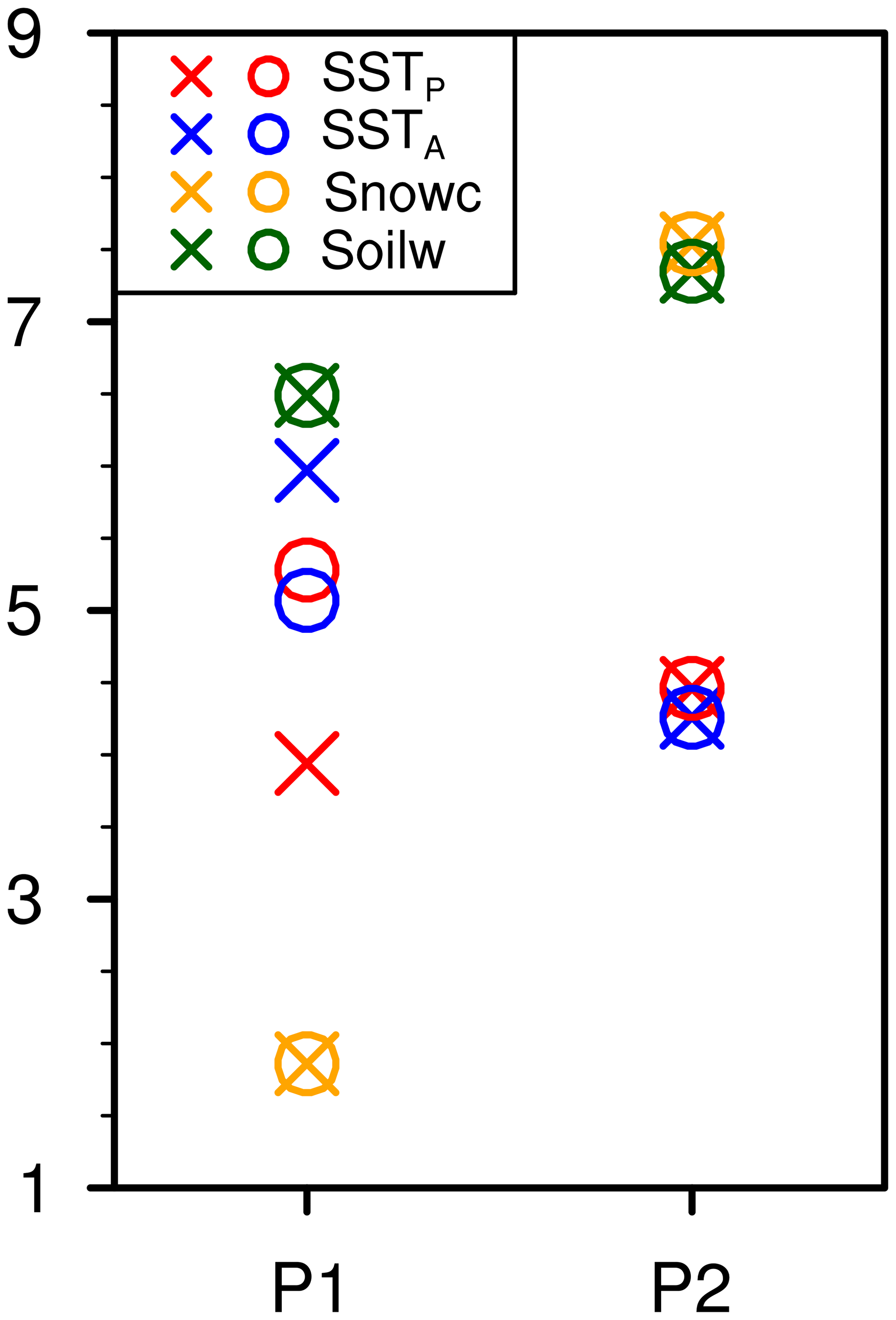
Figure 5 Composite of the simulated HD_NC caused by the four external forcing factors (favored years minus unfavored years). The circles and crosses represent the original and detrended sequences, respectively.

These four indices were employed to linearly fit HD_NC based on a multiple linear regression (MLR) model (Wilks, 2011). As shown in Fig. 4e, the correlation coefficient between the fitted and observed HD_NC was 0.82. After a 5-year running average, the correlation coefficient reached 0.92. This model showed good ability to fit the inflection point in 2010 and highlighted the trend changes. Such a good fitting effect indicates that changes in the four external forcing factors could well have influenced the variation in HD_NC. By exciting stronger responses in the atmosphere, such as the positive EA/WR phase and the strengthened anomalous anticyclone over NC, the abovementioned climate drivers created stable and stagnant environments in which the haze pollution in NC could rapidly exacerbate after 2010 (Table 1). Among the four indices, the correlation coefficients between SST_P and Snowc (Pair 1) and between SST_A and Soilw (Pair 2) were high, whereas the rest were insignificant. The variance inflation factors of the four factors in the MLR model were less than 2, showing that the collinearity among them was weak. When selecting one factor from both Pair 1 and Pair 2 to refit HD_NC, the correlation coefficient between the fitted and observed HD_NC and the trends of the fitted HD_NC in P2 worsened (Fig. S10). Therefore, these four external factors were all indispensable to achieve a better fitting effect. The intercorrelated climate factors of Pair 1 and Pair 2 contributed 27.8 % and 84.6 %, respectively, to the trends of HD_NC in P1 and 54.8 % and 20.4 %, respectively, to the trends in P2. Thus, the joint effect of SST_A and Soilw played a more important role in the decreasing trend of HD_NC in P1; however, the impacts of SST_P and Snowc were more than twice those of SST_A and Soilw in P2. More importantly, the fitted curve revealed a decreasing trend of HD_NC (−5.24 d per decade, passing the 95 % t test) that was larger than the observed value (−4.67 d per decade) during P1. Many studies have noted that human activities have led to persistently increasing trends of HD_NC (Yang et al., 2016; Li et al., 2018). The combination of the exorbitant decreased trend indicated by climate conditions and the long-term trend from anthropogenic emissions resulted in a realistic slow decline (Table 2). This proportion of the trend explained by climate drivers (72.3 %) decreased in P2 because the increasing trend, jointly driven by the climate drivers and emissions, led to a rapid increase in HD_NC.

Table 2 The contribution rate of fitted HD_NC and each external forcing factor to the trend of HD_NC in P1 and P2, respectively.

5 Conclusions and discussion

Haze events in early winter in North China exhibited rapid growth after 2010, which was completely different from the slow decline observed before 2010, showing a trend reversal in the year 2010 (Fig. 1). The trend changes in the associated meteorological conditions exhibited identical responses. After 2010, the lower BLH, weakened wind speed, sufficient moisture and anomalous ascending motion (all with larger tendencies than before 2010) limited the horizontal and vertical dispersion conditions and, thus, enhanced the occurrence of early winter haze pollution (Fig. 2). However, before 2010, the climate conditions showed the opposite characteristics and could create an environment with adequate ventilation for the dissipation of particles.

In this study, the external forcing factors that are closely related to the significant growth of HD_NC after 2010 and the associated physical mechanisms were investigated. These factors might strongly link to the anomalous anticyclone over NC via exciting the EA/WR teleconnection pattern, thereby regulating the meteorological conditions, weakening the dispersion conditions and facilitating the accumulation of haze pollutants. The four climate drivers physically related to HD_NC showed inverse trend changes with an inflection point in 2010, which agrees with the behavior of HD_NC (Fig. 4). The factors of Pair 1 (SST_A and Soilw) and Pair 2 (SST_P and Snowc) had joint effects and played more important roles in the increasing trend of HD_NC in P2 and the decreasing trend of HD_NC in P1, respectively (Table 2). The fitting result of the four factors with the trend of HD_NC showed a strongly decreasing trend in P1 and a weakly increasing trend in P2. In combination with increasing emissions, these factors jointly led to a relatively slow decreasing trend of HD_NC before 2010 and rapid growth afterward. Therefore, both the decreasing trend in P1 and the increasing trend in P2 were caused by a combination of climate drivers and emissions.

Note that a number of factors contribute to the uncertainties in our results. Although a high emission scenario was used to simulate the number of haze days and emphasized the influence of meteorology, no complete and varied emission inventories were used to drive the GEOS-Chem model to make a comparison, which caused certain uncertainty. Furthermore, when assessing the contribution percentages of the external forcing factors, the coupling effect between climate variability and anthropogenic emissions was not considered; therefore, the contribution rate of climate conditions might be overestimated.

For the long-term trend of haze, human activities are the recognized and fundamental driver (Li et al., 2018; Yang et al., 2016). Anthropogenic emissions have exceeded a high level since the 1990s, providing a sufficient foundation for the generation of severe haze pollution (Fig. 1). However, the effects of climate variability delayed warnings before 2010. Together with the local meteorological conditions, the trends of the climate drivers reversed in 2010, initiating a dramatic increase in HD_NC after 2010, which quickened the worsening of haze pollution in NC (Fig. 4e; Table 1). The superimposed effect of high-level human emissions with strengthened climate anomalies loudly sounded the alarms due to the extremely rapid rise of haze pollution.