the Creative Commons Attribution 4.0 License.
the Creative Commons Attribution 4.0 License.
 | 28 Oct 2020
Deep-convective influence on the upper troposphere–lower stratosphere composition in the Asian monsoon anticyclone region: 2017 StratoClim campaign results
Pasquale Sellitto
Francesco D'Amato
Silvia Viciani
Alessio Montori
Antonio Chiarugi
Fabrizio Ravegnani
Alexey Ulanovsky
Francesco Cairo
Fred Stroh
The StratoClim stratospheric aircraft campaign took place in summer 2017 in Nepal (27 July–10 August) and provided for the first time a wide dataset of observations of air composition inside the Asian monsoon anticyclone (AMA). In the framework of this project, with the purpose of modelling the injection of pollutants and natural compounds into the stratosphere, we performed a series of diffusive back trajectory runs along the flights' tracks. The availability of in situ measurements of trace gases has been exploited to evaluate the capability of the trajectory system to reproduce the transport in the upper troposphere–lower stratosphere (UTLS) region. The diagnostics of the convective sources and mixing in the air parcel samples have been derived by integrating the trajectory output with high-resolution observations of cloud tops from the Meteosat Second Generation (MSG1) and Himawari geostationary satellites. Back trajectories have been calculated using meteorological fields from European Centre for Medium-Range Weather Forecasts (ECMWF) reanalysis (ERA-Interim and ERA5) at 3 and 1 h resolution, using both kinematic and diabatic vertical motion. The comparison among the different trajectory runs shows, in general, a higher consistency with observed data as well as a better agreement between the diabatic and kinematic version when using ERA5-based runs with respect to ERA-Interim. Overall, a better capacity in reproducing the pollution features is finally found in the diabatic version of the ERA5 runs. We therefore adopt this setting to analyse the convective influence in the UTLS starting from the StratoClim observations. A large variety of transport conditions have been individuated during the eight flights of the campaign. The larger influence by convective injections is found from the continental sources of China and India. Only a small contribution appears to be originated from maritime regions, in particular the South Pacific and the Bay of Bengal, which, unexpectedly, was not particularly active during the period of the campaign. In addition, a mass of clean air injected from a typhoon has also been detected at around 18 km. Thin filamentary structures of polluted air, characterized by peaks in CO, are observed, mostly associated with young convective air (age less than a few days) and with a predominant South China origin. The analysis revealed a case of direct injection of highly polluted air close to the level of the tropopause (anomalies of around 80 ppbv injected at 16 km) that then kept rising inside the anticyclonic circulation. Due to the location of the campaign, air from continental India, in contrast, has been only observed to be linked to air masses that recirculated within the anticyclone for 10 to 20 d, resulting in a lower concentration of the trace gas. The analysis of a flight overpassing an intense convective system close to the southern Nepalese border revealed the injection of very young air (few hours of age) directly in the tropopause region (∼18 km), visible in the trace gases as an enhancement in CO and a depletion in the O3 one. From the whole campaign, a vertical stratification in the age of air is observed: up to 15 km, the age is less than 3 d, and these fresh air masses constitute almost the totality of the air composition. A transition layer is then individuated between 15 and 17 km, where the convective contribution is still dominant, and the ages vary between 1 and 2 weeks. Above this level, the mean age of the air sampled by the aircraft is estimated to be 20 d. There, the convective contribution rapidly decreases with height and finally becomes negligible around 20 km.
- Article
(4282 KB) - Full-text XML
-
Supplement
(2871 KB) - BibTeX
- EndNote


The upper troposphere–lower stratosphere (UTLS) dynamics of the Northern Hemisphere (NH) during the summer season (June to August) is dominated by the summer Asian monsoon anticyclone (AMA) system (Randel and Park, 2006). In the AMA regions, air masses from the boundary layer (BL) can be effectively uplifted to the UTLS and subsequently transported to the stratosphere, with a vertical transport resulting from the interaction of deep convection with the strong anticyclonic flow of the lower stratosphere (LS) (Randel et al., 2010; Lawrence, 2011). Deep convection can also directly transport air into the stratosphere during intense overshooting events. Once transported into the UTLS, pollutants mainly remain trapped inside the Asian monsoon anticyclone, which acts as a horizontal transport barrier for air masses (Randel et al., 2010; Vernier et al., 2011). High concentrations of tropospheric trace gases as carbon monoxide (CO), nitrogen oxides (NOx), peroxyacetyl nitrate (PAN) and hydrogen cyanide (HCN) were detected by satellite measurements inside the anticyclone borders (Park, 2004; Randel et al., 2010; Santee et al., 2017), while low concentrations of stratospheric tracers were observed (Park et al., 2008; Konopka et al., 2010). Similarly, the AMA also appears as a region of enhanced concentration of water vapour (Forster and Shine, 2002; Dvortsov and Solomon, 2001; Santee et al., 2017), and a model study from Gettelman et al. (2004) suggested that transport related to the AMA could represent up to 75 % of the total net upward flux of water vapour in the summer tropical tropopause layer (TTL). This confinement may favour chemical and microphysical transformations inside its boundaries and may significantly affect the radiative balance and therefore climate at a regional to global scale (Solomon et al., 2010; Sherwood et al., 2010). An additional effect of the convective uplift in the AMA is the formation of the Asian tropopause aerosol layer (ATAL; Vernier et al., 2011), extending between 13 and 18 km over Asia. This layer has been proved to exert a short-wave direct radiative forcing at the top of the atmosphere with values between −0.1 W m−2 (Vernier et al., 2015) and −0.05 W m−2 (Kloss et al., 2019). While it has been demonstrated that the AMA clearly provides an effective pathway for trapping tropospheric pollutants and water vapour in the atmosphere (Ploeger et al., 2013; Vogel et al., 2015), the mechanisms of transport and the distribution of the sources are still not well known (Vogel et al., 2012). A study from Chen et al. (2012) based on Lagrangian model simulations driven by Global Forecast System (GFS) winds suggested that, during the summer season, the BL-to-TTL transport throughout the Asian monsoon regions is dominated by the western Pacific region and the South China Sea. Other relevant sources would include, in order, the Bay of Bengal, South Asian subcontinent and, to a lesser extent, the Tibetan Plateau. Bergman et al. (2013), with a similar Lagrangian approach based on Modern-Era Retrospective analysis for Research and Applications (MERRA) winds, indicated that, at 100 hPa inside the AMA, the main contribution comes from the Tibetan Plateau and India to a similar extent (∼40 % and ∼30 %, respectively) while the western Pacific contributes just ∼10 %. Results from Vogel et al. (2015), based on the analysis of artificial emission tracers from a chemical Lagrangian model for summer 2012, confirmed that the northern Indian subcontinent (with the Tibetan Plateau) and South East Asia (including the eastern part of the Bay of Bengal) represent the most important source regions for the chemical composition of the AMA at the tropopause level. Tissier and Legras (2016), with a study based on backward and forward trajectories on ERA-Interim winds between the top of convective clouds to the tropopause, found that, for the boreal summers of years 2005–2008, the Asian mainland was representing the main source for the AMA composition (∼50 %), followed by the Tibetan Plateau and the North Asian Pacific Ocean to a similar extent (∼20 %).
These studies mostly rely on simulation results, therefore potentially depending on the choice of the driving model setting, while little in situ observational evidence has been collected over this region (mostly from balloon soundings; Bian et al., 2012). The StratoClim aircraft field campaign took place during the end of July to the middle of August 2017 and offered a unique occasion for a detailed in situ sampling of the air composition at the UTLS level of the AMA region during the monsoon season.
Here, starting from the aircraft measurements, we present the convective-source apportionment from the eight flights based on a Lagrangian approach coupled with geostationary observations of convective clouds. The comparison with the in situ measurements is, in turn, exploited to evaluate the capability of the back trajectory approach to capture the convective transport. Using different meteorological input (ERA5 and ERA-Interim as well as kinematic and diabatic vertical velocity), we provide an evaluation of the performance of each setting. A study on the convective transport during the StratoClim campaign is then presented based on the best meteorological framework. The analysis starts from the CO species, used as a tracer for anthropogenic pollution, to characterize the intensity and the timescales of convective transport into the UTLS. A detailed description of the transport processes and of the air composition in terms of convective tracers is presented for two selected flights. These two cases captured the strongest influence of deep convection on the trace gases composition, allowing the characterization of the transport of tropospheric air and demonstrating the potential of the system to capture the transport features in the UTLS from the scale of the anticyclonic circulation to the fine structures of pollution filaments. Finally, we present a statistical analysis, based on all of the campaign flights, of the vertical distribution of convective influence and age of convective air inside the AMA.

Figure 1Campaign flight tracks. (a) Flights 1 (29 July 2017), 3 (31 July 2017), 6 (6 August 2017) and 7 (8 August 2017). (b) Flights 2 (29 July 2017), 4 (2 August 2017) and 5 (4 August 2017). (c) Flight 8 (10 August 2017).
The StratoClim campaign took place in Nepal, based in Kathmandu (27∘42′ N, 85∘19′ E), between the end of July and end of August 2017. Using the M-55 Geophysica aircraft, eight flights were conducted covering the Nepalese and northern Indian region (see Fig. 1). Flights generally lasted between 3 and 4.5 h, mainly sampling the layer between 15 and 20 km. Half of the flights (2, 3, 5, 7) took place during local morning hours, while the other half (1, 4, 6, 8) were conducted during local afternoon hours. More details on the time and altitude of the flights can be found in Figs. 7 and 9 as well as Figs. S1–S6 in the Supplement). Flights 1, 3, 6 and 7 (Fig. 1a) probed the northern Indian area and the southern Bangladesh areas, sampling features of different origin (see Fig. 7 and Figs. S1, S3 and S6 in the Supplement). Flights 2, 4 and 5 sampled air over the Nepalese region at different altitudes (see Figs. 1b and Figs. S2, S4 and S5 in the Supplement). Finally, flight 8 had been designed to fly over a convective system developed at the border between Nepal and northern India (see Figs. 1c and 9c).
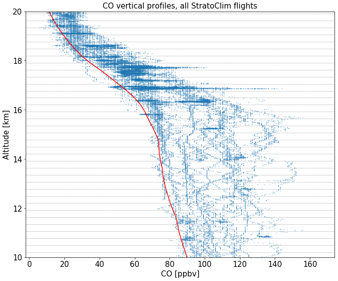
Figure 2Total CO measurements along all eight flights of the campaign. The red line represents the estimated CO background, computed as the fifth percentile of the measurements along the 240 m altitude bins (horizontal thin grey lines).
3.1 CO and O3 measurements from the Geophysica
The high-time-resolution (1 Hz) CO concentration values were collected by the instrument COLD2 (Carbon Oxide Laser Detector; Viciani et al., 2018), installed in the dome on the top of the Geophysica. COLD2 is a quantum cascade laser spectrometer based on direct absorption in combination with a multipass cell. The instrument provides in situ CO absolute concentration values with a relative error of 3 % and a sensitivity of 1–2 ppbv. The CO vertical profiles, recorded by COLD2 during the eight flights of the campaign, are shown in Fig. 2. A background CO concentration (CObase(z0)), in absence of fresh convective transport, is estimated taking the fifth percentile of the CO observations collected for each vertical bin of an array of 50 equidistant levels (z0i) ranging from 8 to 20 km (therefore 240 m between each bin). Ozone concentration, used for the analysis of flight 8 (see Fig. 9), was measured with a chemiluminescent ozone analyser, FOZAN-II (Fast OZone ANalyzer), developed and manufactured by CAO (Russia) and ISAC-CNR (Italy). The instrument is described in detail by Yushkov et al. (1999). This is a fast-response, two-channel automated instrument to measure ozone concentration in the atmosphere from aboard the high-altitude aircraft M-55 Geophysica. This instrument makes use of solid-state chemiluminescent sensors, which are durable enough to provide continuous operation of the instrument for at least 40 h. The instrument has a built-in high-precision ozone generator enabling periodic auto-calibration during the flight. The time response is less than 1 s, and it has a relative error of ≤8 %. Due to technical issues during the campaign, no O3 measurements are available for flights 1 and 7.
3.2 Transport analysis
In the study of atmospheric transport, the Lagrangian approach allows the characterization of the source receptor relation of atmospheric tracers. In the StratoClim framework, we used the TRACZILLA Lagrangian model (Pisso and Legras, 2008), a modified version of FLEXPART (Stohl et al., 2005; Legras et al., 2005), to understand the influence of transport and mesoscale dynamics on the features observed during the flights. Simulations have been based on the simultaneous release of a 1000-back-trajectory cluster, representative of a generic passive tracer, launched in correspondence with the aircraft position. The trajectories have been released with a time step of 1 s along the flight path, travelling back in time for 30 d. The trajectories are bounded to a geographical domain enclosed in a latitude and longitude range of 0–50∘ N and 10∘ W–160∘ E, respectively. When a trajectory crosses these boundaries, it is considered to be terminated. The fraction of the terminated parcels corresponds to the white layer in the colour-coded analysis of convective sources (Figs. 5, 7, 9, 10, 11). The back trajectories have been calculated in four different settings, choosing from ECMWF reanalysis horizontal winds (ERA-Interim and ERA5 at 3 and 1 h resolution, respectively) and kinematic and diabatic vertical motions. Vertical diffusion is represented by a random walk equivalent to D=0.1 as in Pisso and Legras (2008). To individuate the encounter with convective events, diffusive back trajectories have been coupled with high-frequency charts of cloud top altitudes from geostationary satellites (MSG1 and Himawari) as described in the following section. Therefore, a specific geographical bin is indicated as a convective source when, over that bin, a trajectory is found with a pressure higher than the high cloud top pressure, as similarly done in Tissier and Legras (2016). From this analysis we then derive an estimation of the height of convective injection, given from the altitude of encounter between the trajectories and the cloud top height, that would ideally correspond to the main detrainment height. In addition, the time elapsed between the convective cloud encounter and the flight measurements (corresponding to the time of trajectory release) provides an estimate of the age of the air masses. This age is representative of the time elapsed between the detrainment and the capture by the aircraft (and therefore of the age of the air in the UTLS), but we can assume it to be close to the real time of transport from the boundary layer. The unknown in this analysis is indeed the time necessary for the air masses to be uplifted from the boundary layer to the cloud top. As the vertical velocity in a convective updraft of the region may reach 10 m s−1, the time span of the vertical transport would be a few hours (1–2 h) and can therefore be assumed to be the error in the underestimation of the time of transport from the boundary layer. Finally, the possible convective sources will be classified in main source regions as shown in the region mask of Fig. 3.
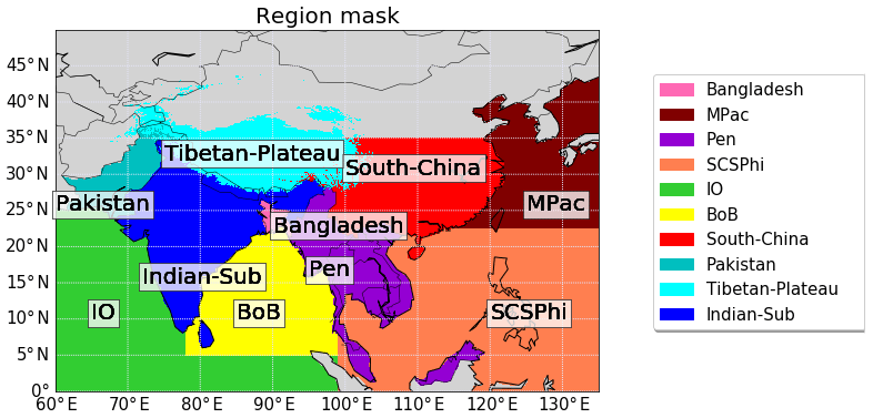
Figure 3Source region mask for the AMA area. In colour: Indian subcontinent (Indian-Sub), Tibetan Plateau (Tibetan-Plateau), South China (South China), Pakistan (Pakistan), South East Asia peninsula (Pen), South China Sea and Philippines (SCSPhi), Bangladesh (Bangladesh), North China (North China), Bay of Bengal (BoB), mid-Pacific (MPac), Indian Ocean (IO).
3.3 Geostationary retrieval of cloud top: MSG1 and Himawari
The cloud top height is taken from the cloud top temperature and height (CTTH) product, developed within the European Organisation for the Exploitation of Meteorological Satellites (EUMETSAT) Satellite Application Facility (SAF) on Support to Nowcasting and Very Short Range Forecasting (NWC) products (Schulz et al., 2009; Derrien et al., 2010). To cover the whole domain of interest, we make use of the CTTH product from both the MSG1 images for longitudes west of 90∘ E and the HIMAWARI-8 images for longitudes east of 90∘ E. The MSG1 satellite, operated by EUMETSAT and relocated at 41.5∘ E after 4 July 2016, carries the Spinning Enhanced Visible and Infrared Imager (SEVIRI), an optical imaging radiometer. A detailed description of MSG1 can be found in Schmetz et al. (2002). The SEVIRI instrument has three visible–near-infrared solar channels (0.6, 0.8 and 1.6 m), eight thermal infrared channels (3.9, 6.2, 7.3, 8.7, 9.7, 10.8, 12.0 and 13.4 µm) and one high-resolution visible channel (0.4–1.1 µm). The nadir spatial resolution of SEVIRI is 1 km for the high-resolution visible channel and 3 km for the others, with a frequency of image collection of 15 min. HIMAWARI-8 is a geostationary meteorological satellite launched by the Japan Meteorological Agency (JMA) on 7 October 2014, and it is centred at 140∘ E, covering the East Asian and western Pacific regions. The visible–infrared radiometer onboard (Advanced Himawari Imager, AHI) has 16 observational bands: 4 bands in the visible and near-infrared spectrum (0.47–0.86 µm), 2 bands in the short-wave infrared (1.6–2.3 µm), 1 band in the medium-wave infrared (3.9 µm), and 9 bands in the thermal infrared (TIR) region (5–14 µm). It has a nadir spatial resolution of 500 m and 1 km in the visible range and 2 km in the IR, and the observations are collected at 10 min intervals. For computational reasons, we use here one image every 20 min. For the processes we are considering, this does not significantly affect the results of the analysis.
The cloud analysis algorithm for the CTTH product includes methods for the identification and property retrieval of multi-layered cloud systems and the determination of cloud thermodynamic phase based on an algorithm that incorporates numerical weather prediction model profiles to input vertical atmospheric profiles into a fast radiative transfer model (RTTOV from Met Office; Saunders et al., 1999). The estimate of the cloud top height is based on different approaches, including a best fit between the simulated and the measured 10.8 µm brightness temperatures, the H2O–IRW (in the IR window) intercept method (Schmetz et al., 1993), and the radiance-rationing method (Menzel et al., 1983). The techniques used to retrieve the cloud top height depend on the cloud type (CT product). The CT discrimination is performed by a multispectral threshold method applied on the identified cloudy pixels using the various channel combinations. This product classifies major cloud classes: fractional clouds; semitransparent clouds; and high, medium and low opaque clouds. More details on the retrieval algorithm can be found in Stengel et al. (2014), Finkensieper et al. (2016) and the Algorithm Theoretical Basis Document (ATBD) Meteo-France (2016) document (http://www.nwcsaf.org, last access: 13 November 2019). A comparison of the SAF-NWC product with spaceborne active lidar measurements can be found in Sèze et al. (2015). Here we use a specific version of the product where the ancillary data are taken from ERA5 at hourly resolution. For the scope of our analysis, we selected the highest and opaque cloud classes (high opaque clouds, very high opaque clouds and very high semi-transparent thick clouds) that are representative of the deep-convective events as classified in the cloud type (CT) product.
3.4 Kinematic vs. diabatic approach and ERA-Interim–ERA5 comparison
3.4.1 Spatial distribution of sources
One of the potentially largest uncertainties in the study of Lagrangian modelling is the representation of vertical transport. The most common methods for estimating the vertical motion are the kinematic approach, which computes vertical velocities from mass conservation, and the diabatic approach, which uses diabatic heating rates as vertical velocities in a coordinate system with potential temperature as the vertical coordinate. Usually vertical velocities from reanalysis are noisy, and strong dispersion was observed in the kinematic trajectories (Ploeger et al., 2010, 2011; Schoeberl and Dessler, 2011), with unrealistic transport characteristics such as excessive or too low age of air in the stratosphere (Schoeberl and Dessler, 2011; Diallo et al., 2012). At the same time, previous studies based on ERA-Interim wind fields and heating rates in the AMA region suggested a higher reliability of the diabatic heating rates for convective transport to the TTL (Ploeger et al., 2011; Bergman et al., 2015) as well as higher vertical motion in the inner tropical pipe region (Hoppe et al., 2016). In order to evaluate the sensitivities and estimate the uncertainties associated with vertical velocities, we compare kinematic and diabatic trajectories. Moreover, we test both ERA-Interim ( horizontal resolution, 3 h temporal resolution and 60 vertical levels) and the newer ERA5 dataset at higher spatial and temporal resolution ( horizontal resolution, 137 vertical levels and 1 h temporal resolution). In both cases the vertical velocities are taken as an instantaneous field for the kinematic computation, while for the diabatic computation, the heating rates are only available as averages of the reanalysis time step. The diabatic vertical velocities in this paper are estimated making use only of the radiative heating term, which represents the dominating contribution in the UTLS region (Ploeger et al., 2010).

Figure 4Convective-source distribution identified by the trajectories for the whole aircraft campaign. The probability per square kilometre of finding a source over a specific area is computed as the fraction of parcels that encounter a convective cloud there with respect to the total number of released parcels. The plots are in logarithmic scale. The percentage in the title indicates the fraction of convective parcels integrated over the whole surface. (a) Convective-source distribution obtained with ERA5 meteorology and kinematic vertical motion (EAZ); (b) ERA-Interim meteorology and kinematic vertical motion (EIZ); (c) ERA5 meteorology and diabatic vertical motion (EAD); (d) ERA-Interim meteorology and diabatic vertical motion (EID).
Figure 4 shows the probability distribution of all the convective sources individuated by the back trajectories run for the whole ensemble of flights, corresponding to the different meteorological inputs (ERA5 and ERA-Interim, abbreviated EA and EI, respectively) and the different vertical velocity computations (kinematic and diabatic, indicated by Z and D, respectively). The comparison among the runs shows a general consistent pattern, with some differences when comparing EA with EI. In particular, EI runs show an increased probability of detecting convective sources in the maritime regions (Pacific Ocean and Bay of Bengal) with respect to EA runs and less convective sources in the Tibetan Plateau area. A higher number of convective sources is also found in northern China in the EI. Comparisons between D and Z runs, for both EA and EI, does not show significant differences in the distribution of the sources. A higher percentage of detected convective parcels is nevertheless found in the diabatic run with respect to the kinematic computation, and while in EA the difference is of a few percentage points, in EI the gap between D and Z is higher (∼15 %). This difference is mainly due to the faster uplift in EID linked to the strong heating rates, while in EIZ the vertical motion is slower and more diffusive. More details on this comparison, based on a larger ensemble of simulations, will be discussed in a future paper. Very recent work from Li et al. (2020), also showing a comparison between EAD, EAZ, EIZ and EID from two balloon soundings, found a faster vertical transport in EA than in EI in both D and Z runs. While this is consistent with our results in the kinematic version, we find more convective influence in the EI diabatic run with respect to the EA diabatic run. It has to be noted however that here the amount of convective influence is not just linked to the vertical transport from the wind fields but is also strongly related to the spatial distribution of convective clouds from observation: differences in the horizontal winds in the model may therefore lead to a change in the number of convective encounters in the results. A more detailed and systematic study on the vertical transport can be found in Legras and Bucci (2020).
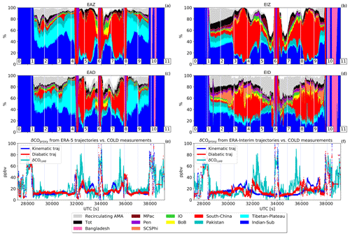
Figure 5Convective-source contributions in the ERA5 (left column) and ERA-Interim (right column) computations along the flight time of F6 (6 August 2017). The thickness of each coloured layer in (a)–(d) represents the percentage of contribution of the region associated with the colour code shown in Fig. 3. The grey layer indicates the percentage of parcels recirculating inside the Asian monsoon anticyclone without hitting convection. The thickness of the black layer indicates the percentage of contribution from sources different from the ones identified in Fig. 3. The remaining white layer represents the percentage of parcels that exited the boundaries of the domain before encountering any convective cloud. Panels (e) and (f) show the time series of the CO anomalies δCOcold (in green) measured by the COLD2 instruments compared to the artificial CO enhancement δCOproxy simulated from both the kinematic (blue) and diabatic (red) computations. Numbers on the panel punctuate the flight path on equally spaced time intervals, corresponding to the position of the flight, as shown in Fig. 7b.
3.4.2 Convective-source analysis and comparison with CO measurements
Here, we exploit the results of the StratoClim campaign to assess the performance of each reanalysis setting driving the simulations. To understand the capability of the trajectory system to reproduce small-scale transport features, we compare the temporal evolution of the simulated convective contributions with the measured CO from the COLD2 instrument. As a representative case we discuss here the performances of the trajectory analysis for F6 (6 August 2017), while the dynamics and the features observed in this flight are further examined in Sect. 4.1.2. During F6, the aircraft performed a long leg at a constant altitude (around 16.9 km, in the upper troposphere), travelling in a south-east direction towards Bangladesh and then turning back along the same path at the same altitude. In this transect the aircraft encountered a plume of pollution that appears as a distinguished isolated feature (Fig. 5e–f; around seconds 32 000 and 36 000). Overall, all the four simulations indicate that the plume has been convectively injected in the upper troposphere from the South Chinese region (see Fig. 5a–d). Comparing the two reanalysis results, ERA5 shows a higher consistency in the evolution of the feature with respect to ERA-Interim. The latter seems in fact to individuate the plume at a northern position with respect to the measurements (segments 3–4 and 8–9 of the flight). Moreover, the consistency between Z and D results is not the same for EI and EA. The EID run, for instance, returns noisier results with respect to EIZ as well as a higher fraction of recirculating air (grey shade) and notable differences in the relative contribution of the sources as a function of time (Fig. 5b and d). In the case of EAD and EAZ runs instead, there are no meaningful discrepancies in the spatial and temporal structure of the plume, and the main differences are found solely in the relative amount of contribution from the possible sources. According to the EAD simulations, for example, the Chinese component of the plume between segments 5–6 and 7–8 represents around 20 % of the total composition, while for the EAZ, such a percentage rises to 80 % (Fig. 5a and c).
In order to have a more quantitative estimate of the quality of the different approaches, we compared the CO measurements from COLD2 with an estimated concentration derived from the simulations performed along the flight path. For each time step along the flight, the back trajectory analysis indicates the geographical distribution of the convective sources. To take into account the spatial heterogeneity in emission intensity, we multiplied the convective distribution by the CO fluxes from an emissions database. We used here the 2010 monthly emissions from the MIX v1.1 gridded emissions database (M. Li et al., 2017) based on a harmonization of different up-to-date Asian regional emission inventories. The quantity we obtain (δCOTrac(z(t))) is therefore indicative of the CO mass potentially transported from the BL up to the flight position, hence the enhancement of CO with respect to the background. With our diagnostic, it is not possible to pursue a rigorous computation of the CO mixing ratio since the simulation does not take into account all the processes of microphysics and chemistry. We therefore adopted an empirical rescaling as explained in the following.
Figure 2 shows the total CO observations (COcold(z)) along the vertical profiles, collected during the whole campaign. For each vertical bin z0i we computed the mean CO enhancement δCOcold(z0i) with respect to the CObase(z0i) baseline (as defined in Sect. 3.1).
Similarly, for each point along the flights, we compute the δCOTrac(z(t)) quantity and, for each vertical bin, its average on the whole ensemble of measurements .
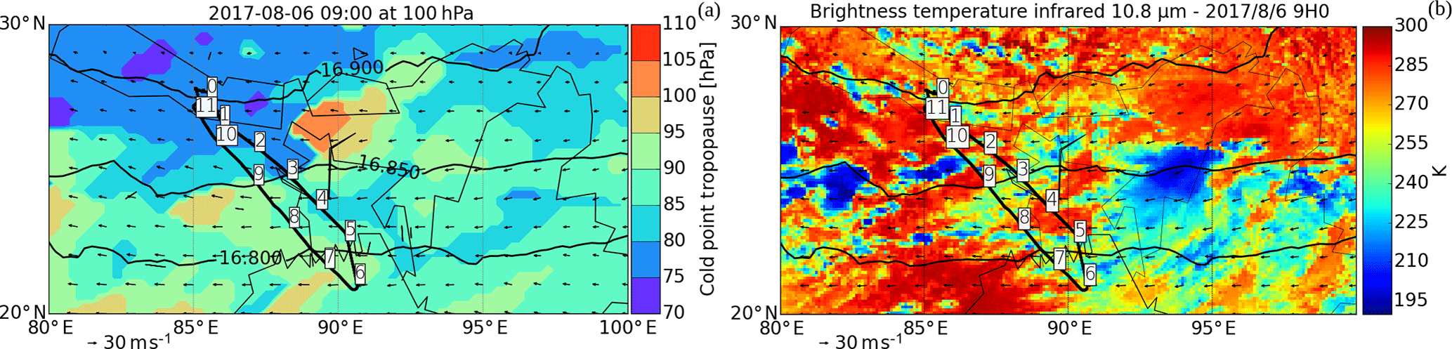
Figure 6(a) Cold-point pressure, wind speed and direction, and geopotential contours from ERA5 at 100 hPa for 6 August at 09:00 UTC (around the middle of flying time of F6). (b) Brightness temperature at 10.8 µg from the MSG1-Himawari observations at the same time as in (a). The black line traces the complete flight track. The numbers on the track punctuate the flight path at equally spaced time intervals, corresponding to the numbers shown in Fig. 7d.
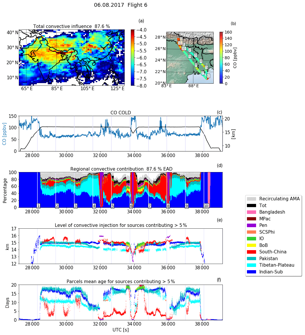
Figure 7Back trajectory analysis of convective sources for F6 (6 August 2017). (a) Convective-source-region distribution. (b) CO concentration along the flight track. The numbers along the flight track correspond to the numbers along the time series of panel (d). (c) CO concentration along the path of flight (in blue) and altitude of the flight (black). (d) Convective-source contributions along the flight. The colour is referring to the region colour code of Fig. 3 plus the non-convective air recirculating inside the AMA (grey shade) and the remaining convective sources (black). (e) Level of injection for convective sources contributing 5 % of the total convective air. This level is computed as the height at which the trajectory is first found below the convective cloud top. (f) Age of the convective air for convective sources contributing for 5 % of the total convective air. The age is computed as the number of days between the trajectory release and the encountering of a convective cloud.
The parameters and are therefore representative of the relative CO enhancement at a given altitude with respect to the campaign average enhancement, as evaluated by the simulations and the measurements, respectively.
We therefore define our CO enhancement proxy from TRACZILLA as
We want to emphasize that this approach is not intended to give a quantitative method for computing CO anomalies in the atmosphere. It is instead an empirical quantity that can be directly comparable to the observations to check for the correct identification of the pollution plumes.
Results for F6 are shown in Fig. 5e and f. Again, the results from ERA5 (Fig. 5e) show a better consistency with the measurements and a better coherence between the kinematic and diabatic versions. The simulation presents a correct timing in the capture of the plume (between points 4 and 8), with a signal enhancement compatible with the measured one. The Pearson correlation coefficients (R) between the simulated and the measured values of CO anomalies are 65.7 % and 67.7 % for the kinematic and the diabatic runs, respectively. In the ERA-Interim version (Fig. 5f) the relative enhancement between outside and inside the plume is damped, and the timing is not consistent with the observations. This is particularly visible in the kinematic computation (that has in fact the lowest correlation coefficient, 49.4 %), while the diabatic one looks closer to the COLD2 measurements (with a correlation of 56.4 %).
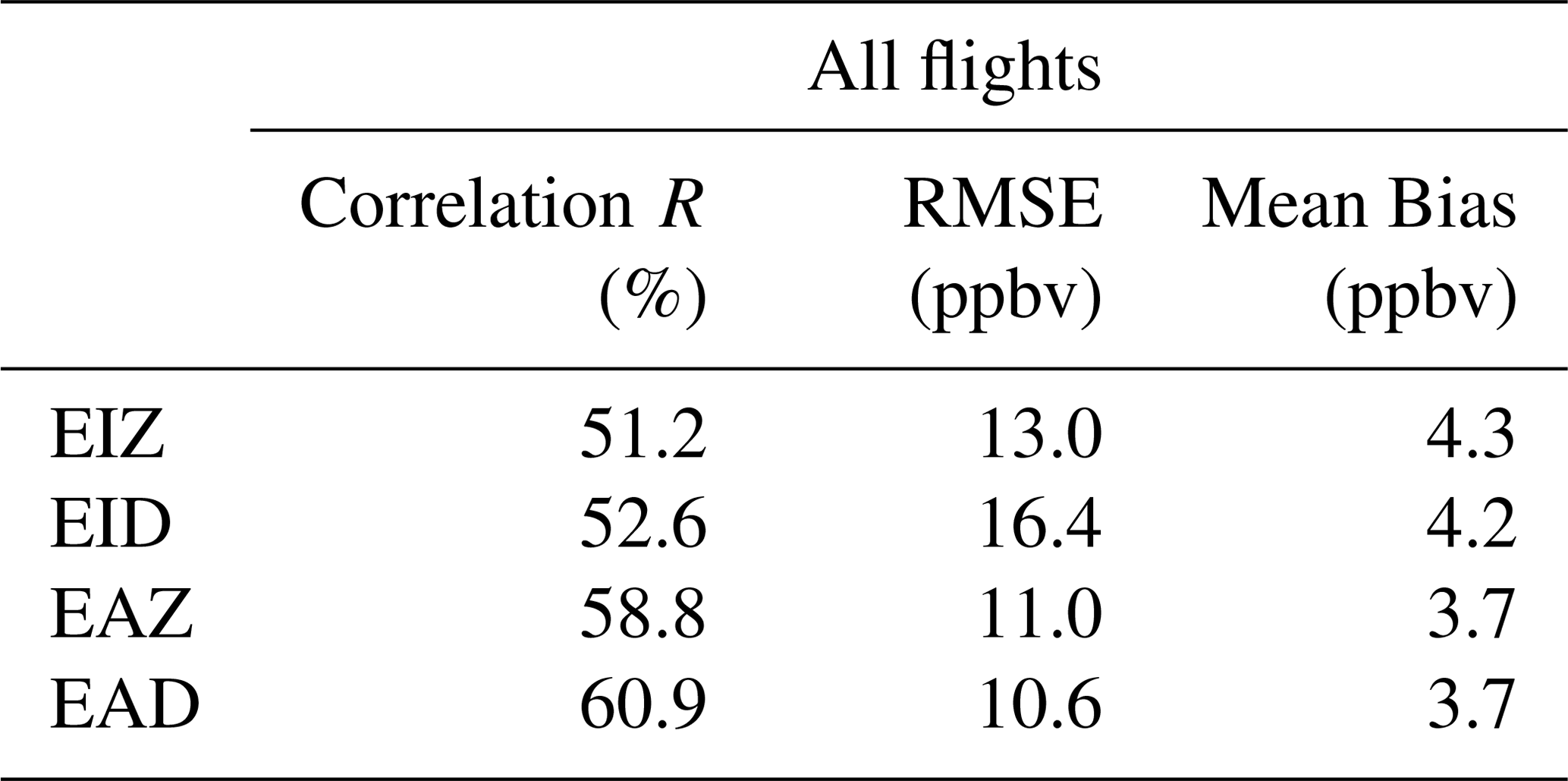
The results of the statistics are shown in Table S1 of the Supplement for each single flight and in Table 1 for the whole campaign average. The correlation analysis confirms that ERA5 performs better than ERA-Interim in reproducing the trace gas transport to the UTLS (R of around 60 % vs. 50 %). In both EA and EI, the diabatic vertical transport better reproduces the variability observed in the CO measurements, with a slight enhancement in the correlation with data with respect to the kinematic simulations. In the EI version, though, the diabatic computation shows a higher RMSE due to the noisy nature of the output signal. Overall, the EAD approach appears to perform the best, with the highest R correlation coefficient (60.9 %), lowest root mean square error (10.6 ppbv) and lowest mean bias (3.7 ppbv) with respect to the other approaches. The interpretation of the convective transport influence that follows is therefore based on the ERA5 diabatic simulations.
Table 1Correlation coefficient, root mean square error and mean bias between δCOproxy(z(t)) and δCOcold for the different meteorological settings (EAZ, EAD, EIZ, EID). Values are averaged on the results from all the eight flights.
This section provides a detailed discussion of the transport properties for two noteworthy cases of convective influence observed during the campaign: F6, which provides a clear case of deep-convective injection of fresh pollution in the upper troposphere, and F8, in which the aircraft first flew over an extended continental convective system, sampling air from both fresh and old convection, and later captured an older plume of clean oceanic air injected into the UTLS by a typhoon system.
4.1 Flight 6, 6 August 2017: convective outflow of Chinese pollution
4.1.1 Meteorological condition
F6 took place under the condition of unimodal anticyclone (i.e. a circulation revolving around a single centre; see Fig. S7f in the Supplement). The geopotential contours at 100 hPa show a circulation centred around 33∘ N and 90∘ E, close to the flight track position (20–26∘ N and 85–90∘ E). F6 therefore sampled the inner part of the AMA. The cold-point pressure in the region of the Geophysica sampling was between 85 and 95 hPa (from ERA5; see Fig. 6a), right above the level of the flight. The mean winds around the flight position were purely easterlies, transporting air from the centre of South China along the anticyclonic circulation. No close intense convective system was detected, with the exception of the one at 92–95∘ E (see Fig. 6a). The influence of transport from these clouds would eventually be observed as young air from the Indian subcontinent, but, as indicated by the trajectory study in the next section, the flight did not capture any influence from this region.
4.1.2 Air mass source apportionment
During F6 (see Fig. 7b) the aircraft flew at a nearly constant altitude, around 16.9 km (∼98 hPa), going from Kathmandu toward the Bay of Bengal in a south-east direction. In addition, the aircraft performed a dive at 15 km over the Bangladesh coast, measuring a CO peak of 160 ppbv (at 34 000 s; black line in Fig. 7c). The source contribution analysis from the trajectories (Fig. 7d) shows a dominance of northern Indian air (∼40 % of air composition) mixed with clean Tibetan convective air (varying between ∼20 % and ∼40 %) for the lower CO concentration regions. This air is characterized by air injected at 15 and 14 km (Fig. 7e) and an average age of the order of 2 weeks and 10 d, respectively (Fig. 7f). Those air masses had circulated around the anticyclone before being sampled by the aircraft. The CO mixing ratio measured at this altitude varied between 60 and 80 ppbv while flying north of 24∘ N but increased up to 140 ppbv when arriving around 23∘ N (between flight points 4–5 and 7–8; see blue line in Fig. 7c). This pollution plume is characterized by three distinct peaks. The more external ones (and therefore the northern filament) reach a CO concentration of 120 ppbv (at 32 000 and 36 000 s), composed 100 % of convective air of a few hours of age (∼6 h) coming from the South East Asia peninsula region, and the analysis reveals that this air has been injected at a very high altitude (16 km, among the highest injection altitude detected for the StratoClim campaign). Looking at the more detailed distribution of sources in correspondence with this region (Fig. 7a), we found that the convection over the Asian peninsula was mainly located in north-central Myanmar. The analysis suggests that this filament is overlapping with another thin plume of pollution from South China, similarly very fresh (age around 1 d). The second filament is detected at around 33 400 and 35 500 s and brings the most polluted air (around 140 ppbv) associated with a dominance of convective South Chinese air (>80 % of contribution) with a longer average age of transport (around 2 d). This second filament originated mainly around the Sichuan Basin (see the maxima around 105∘ E in Fig. 7a), a very polluted region of China, with an injection level of around 15.5 km. The third and weaker filament is observed at around 33 000 and 35 200 s and is characterized by a CO concentration of around 90 ppbv. This is composed mainly of a mixture of ∼17 d old Indian air (30 %) and 3 d old South Chinese air (20 %) that a more detailed analysis shows to be injected from a western region of South China (at 112∘ E). The highest CO peak in the middle of the flight (flight point 6) is instead linked to very fresh pollution captured during the deep dive down to 15 km. The plume has an age of transport of the order of a few hours, coming from the Pen region and South China and transported from low level injection (around 13 km). It is interesting to note that this peak is not simply related to the change in altitude since, as shown in Fig. 5a, the enhancement in CO is still present even when the height-dependent background profile is subtracted.
From a more detailed analysis of the geostationary satellite images (not shown), those high-injection events turn out to be very localized (convective-cloud dimensions of the order of 1∘) and fast-developing (persisting for a period of around 2 h), injecting air directly into the upper troposphere. This pollution is then advected horizontally by the anticyclonic circulation ascending at the same time, following the upward large-scale pattern suggested by Vogel et al. (2019). The total vertical displacement between the convective injection of air and the moment of observation is 2 km for the Chinese air in a time frame of 2–3 d and ∼1km for the South East Asia peninsula air in a time frame of 5–7 h, faster with respect to the estimated average radiative heating rate (Wright and Fueglistaler, 2013). The analysis of this specific flight reveals how mass samples at 16.9 km can reach up to 100 % fresh convective air composition and anomalies of CO up to 90 ppbv. This happens during a weaker phase of convection over the region, indicating that, throughout the whole monsoon season, deep convection may play a relevant role in the composition of the UTLS, transporting young and heavily polluted air masses directly close to the tropopause level.
4.2 Flight 8, 10 August 2017: tropopause crossing, overshoots and typhoon plume
4.2.1 Meteorological condition
F8 took place during a more extended phase of the anticyclone, when the core was shifted westward, with an Iranian mode stretching to 20∘ E, a central mode positioned between 60 and 80∘ E, and a Japanese mode extending to 150∘ E (see Fig. S7h in the Supplement). During this flight, the aircraft sampled the inner part of the central mode in a region where the cold-point pressure was varying between 85 and 90 hPa (see Fig. 8a). In this case, during the flight leg between segments 3 and 8, the flight was crossing the tropopause (altitude around 86.5–87.5 hPa). Moreover, between segments 2 and 5, the aircraft was passing close to the intense convective system visible in Fig. 8b, south of the Nepalese border. Winds in this part of the flight were mainly north-easterly due to the westward shift of the anticyclonic centre.

Figure 8As in Fig. 6 but for F8 (10 August 2017) at 10:00 UTC (around the middle of the flight).
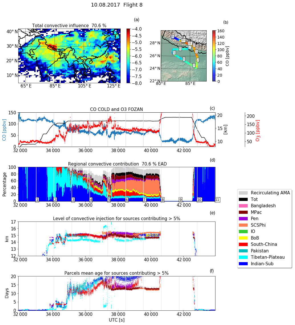
Figure 9As in Fig. 7 but for F8 (10 August 2017). Panel (c) also reports the O3 concentration from the FOZAN instrument (not available in F6).
4.2.2 Air mass source apportionment: convective overshoots
This flight chased the intense convective system which developed over the Ganges valley in the early afternoon hours (as seen in Fig. 8). The aircraft flew in a segment parallel to the Nepalese border (see Fig. 9b; segments between 3 and 8) at a nearly constant altitude of 17.7 km (∼86 hPa), with a final segment (between points 8 and 10) at 19.1 km (∼68 hPa) over Nepal. It is worth noting a progressive decrease in the CO concentration during the constant altitude segment between points 2 and 5, with values decreasing from 80 ppbv to below 60 ppbv (Fig. 9c). This corresponds, in the analysis, to a progressive decrease in the total convective influence (Fig. 9d), from a 100 % to around 50 %. On the other hand, an increase in the fraction of recirculating parcels (trajectories that travel inside the AMA region for 30 d back in time without encountering any convective influence) is detected. For this flight, the O3 concentrations from the FOZAN instrument are also available (red line in Fig. 9c), showing an increasing mixing ratio from around 120 to around 150 ppbv in anti-correlation with CO. These observations suggest an increasing mixing of stratospheric air in the sampled region while travelling north. This is likely due to a progressive crossing of the tropopause, whose pressure level was close to the level of the flight, in particular right after point 4 (Fig. 8a), where the trajectories also find the lowest tropospheric influence. From point 2 to point 4 of the flight, according to the trajectory analysis, the observed convective air is a mixture of air coming from India (50 %; northern side, as visible Fig. 9a) and Tibetan Plateau air (25 %–30 %). Most of the convective sources are located near the Himalayan barrier. This air, injected at 14 km (Tibetan air) and 15 km (Indian air), took a long time to travel from the injection points to the flight position (about a couple of weeks; see Fig. 9e and f). The situation slightly changes between points 4 and 5: the total contributions of Indian and Tibetan air decrease to less than 25 %, with a contribution from the Tibetan Plateau of a few percentage points, comparable to other minor sources, such as South China. While the flight is travelling northward, it samples increasingly old air, with ages growing from 10 d to up to 20 d. The recirculating air contribution in this segment is up to 20 %. This reflects the low values of CO, which went down to 55 ppbv in this part of the flight. At the end of this segment, close to point 5, a peak of CO is observed (reaching more than 90 ppbv). This peak is also individuated by the trajectories that indicate a total convective activity of 80 %, dominated by the contribution of the Tibetan Plateau (around 40 %). This air, contrary to the surroundings, is injected at a higher level (>16 km) and has a younger age (around 2.5 d). Immediately after this signature, the flight encounters an air mass of stratospheric origin, visible in the CO concentration drop to less than 50 pbbv and the corresponding enhancement in the O3 measurements (up to 200 ppbv) and reflected in the decrease in the total convective influence. According to the analysis, all the air sampled during this flight was fairly old, with average ages between 10 and 20 d (with the exception of the peak close to point 5). This may seem contradictory with respect to the close position of the flight to the convective system shown in Fig. 8b. The flight level, though, was quite high with respect to the main cloud top height of this system (around 86 hPa compared to cloud tops identified on average at around 100 hPa). Nevertheless, a more detailed analysis reveals that, in some points, the flight was able to capture some very intense overshoots and convective outflows from very fast and localized plumes. These are hardly recorded by the infrared channels of MSG1, but their effects are visible as small peaks in CO centred around the points 34 700, 35 500, and 36 250 s. The comparison with the satellites' visible images (not shown) suggests that those weak enhancements are associated with very young outflows, of the order of a few minutes to less than 1 h. A further young outflow contribution is identified at around 37 200 s, overlapping the older air plume of point 5. Being the flight in this tropopause-crossing region, it means that the convective events were actually penetrating the tropopause level. Those events happened at a very small temporal and spatial scale, and therefore the convective analysis based on the SAF products (that have coarser resolution; see Sect. 3.3) is not always able to discriminate them. Those very fresh outflows have important effects on the microphysics of the UTLS and deserve a dedicated deeper analysis. A thorough discussion of these events, based on the higher-resolution visible images from the geostationary satellites and additional in situ data, will be presented in a future paper.
4.2.3 Air mass source apportionment: typhoon injection
After point 5, at the same flying level as the previous segments, the measurements showed a sudden change in the trace gas concentrations. Between points 5 and 8, the flight spanned an extended region of low and nearly steady values of CO, varying between 60 and 70 ppbv, and O3 concentration, decreasing from 135 ppbv to 100 ppbv. This change is also reflected and explained by the trajectory analysis: this air appears to be associated again with a high fraction of convective influence (up to 80 %) and in specific with a dominant fraction of old (15 d) convective air from the South China Sea and Philippines (SCSPhi) region (∼40 %), with sources mainly concentrated over the southern coast of China. As can also be seen from the geostationary brightness temperature images (not shown), those sources are related to a typhoon system named Nesat. This typhoon persisted over the ocean for several days (from 25 to 30 July) and injected air at around 15 km. This system carried clean air that mixed with a fraction (∼10 %) of old (∼12 d) and likely slightly polluted air from South China and the South East Asia peninsula. In this section of the flight we reach a of convective influence of up to 80 %, the highest fraction detected at this altitude during the campaign, strongly dominated by the oceanic contribution (SCSPhi+MPac). After point 8 the plane rose up to 19.1 km (∼68 hPa), entering completely into the stratosphere. This reflects a sharp increase in the O3 concentration (up to 400 ppbv) and decrease in the CO mixing ratio (between 20 and 30 ppbv). No convective influence is found in this flight segment. According to the trajectory analysis along this ascending segment and to the following descent, the influence of air from the typhoon injection extended from 17 km up to 19 km. While during the whole campaign the other convective contributions at this level were on average 20 d old, this case represents an exception, with a large fraction of air masses related to an age of 11–12 d.
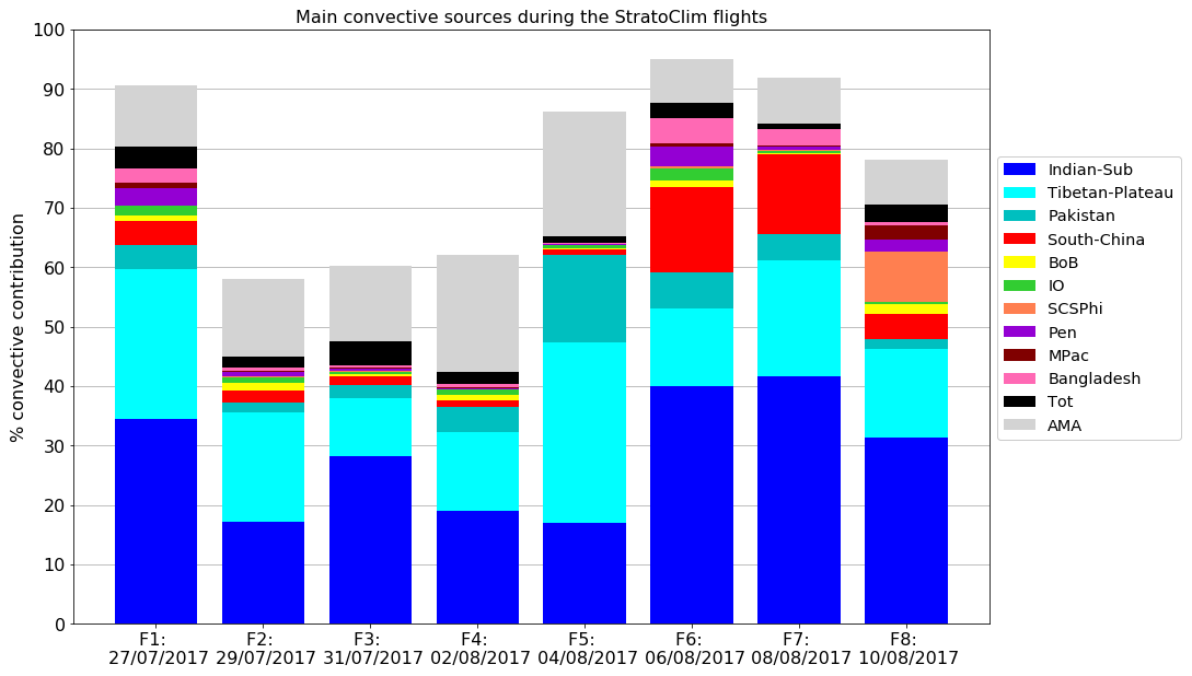
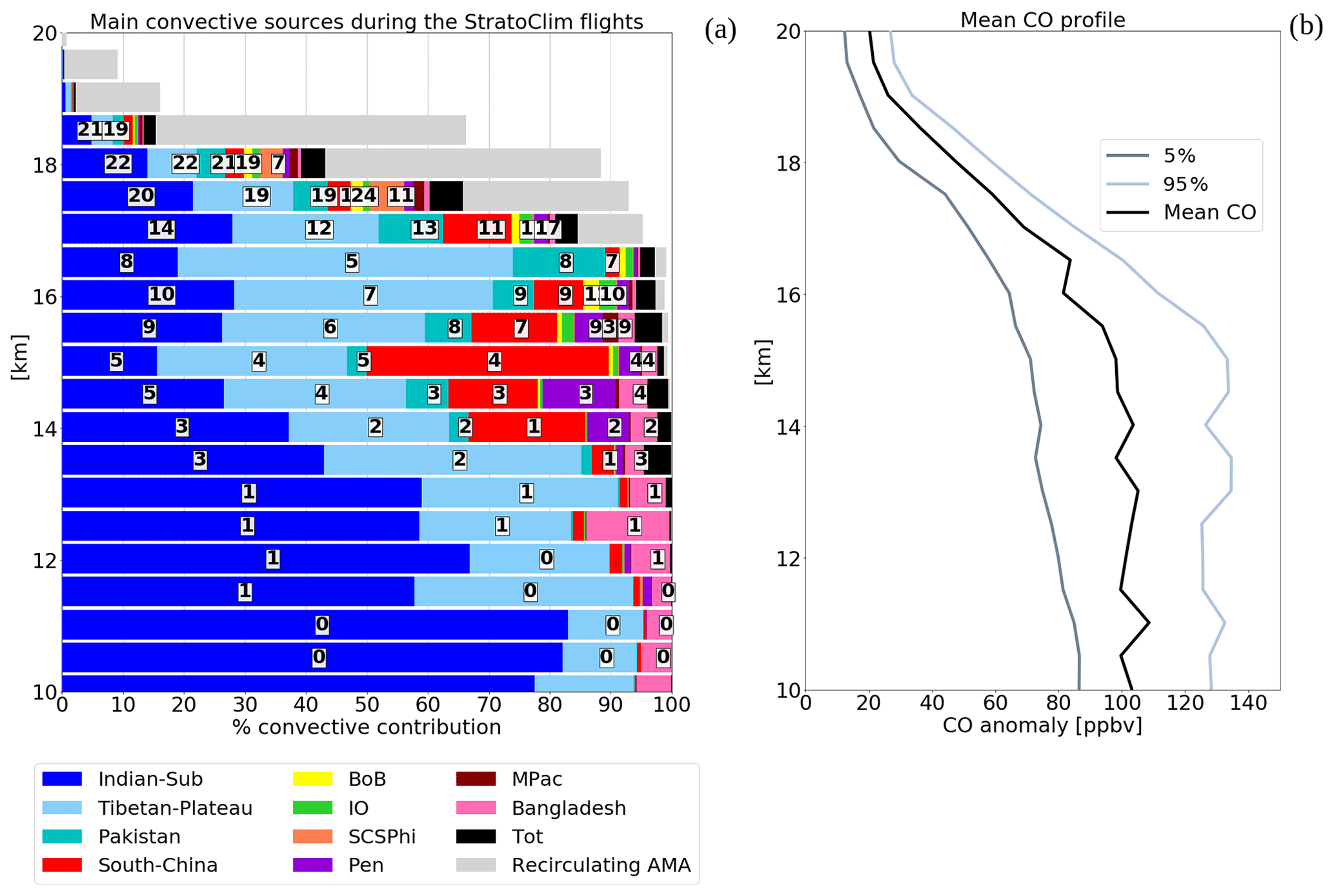
Figure 11(a) Vertical distribution of convective influence as individuated from the trajectories through the whole campaign. Colours indicate the different regions as in Fig. 3, and the numbers indicate the mean age of transport for each source region at that height bin. (b) Mean CO concentration (black) and the 5th (dark grey) and 95th percentiles (light grey) for the different height bins, as seen by the COLD2 instrument through the whole campaign.
4.3 Average convective influence for the whole campaign
A similar analysis was carried out on all the campaign flights. Figure 10 shows an overview of the main convective sources observed. The campaign took place in a break phase of the monsoon, characterized by less precipitation and less convective activity with respect to the average, except for the last days (after 6 August), when some intense (but isolated) convective systems were observed. This is also reflected in the total convective influence observed by the different flights. In flights F2 through F5, when a large part of the track was above 17 km, the observed convective influence was limited to less than 50 % and to around 60 % for F5, with a strong dominance of local air coming from the Indian subcontinent, especially the northern part, and the Tibetan Plateau (also visible in Fig. 4c). In the first and the last three flights a larger variability of sources was instead observed, with a total convective contribution larger than 70 %. F6 and F7 also show a non-negligible contribution from the South China region (dominated by convection from the Sichuan area and west-central China; Fig. 4c), bringing polluted air to the UTLS level. Contrary to the expectation, almost no maritime air was observed, except for the last flight, F8, which sampled the outflow from the typhoon mentioned in Sect. 4.2.2 (dark orange shade in Fig. 10). Overall, during the campaign the Geophysica sampled a prevalence of convective air from the Indian subcontinent with an average influence on the air composition of around 20 %–30 %. Another big contributor is represented by the Tibetan Plateau. The observed convective influence is strongly dependent on the region investigated by the aircraft. In fact, we observed a higher contribution of the Tibetan Plateau (up to 30 %) during the flights that were operating over Nepal. Two additional relevant sources of convective air are South China and Pakistan, with a contribution varying according to the synoptic conditions and the sampled region. In correspondence with both source regions, we generally observed an enhancement in pollutant concentration, both being representative of highly emissive areas. The total contribution from regions other than those selected in the mask of Fig. 3 is, for each flight, negligible (black shade, between 0.2 % and 0.8 %). Figure 11a illustrates the convective influence along the vertical, as observed by the totality of flights, compared with the corresponding observed mean CO (11b) over the same level bin. The analysis shows that, on average, below 15 km the sampled air is mostly of convective origin (close to 100 %) and very young (age below 3 d). It should be noted, however, that the total measurements at those heights are below 1000 samplings (that means less than 1000 s of measurements out of around 93 000 s of total data collection); therefore the relative source apportionment may not be statistically significant with respect to the above levels (see the vertical distribution of sampling in Fig. S8 in the Supplement). Between 15 and 17 km, close to the level of the tropopause, convection still plays a predominant role, with a percentage of influence greater than 90 % and an average time of transport of the order of 1 week. In this layer, the average CO anomaly is about 25 ppbv over the background (that we again estimate by the fifth percentile; dark grey shade), with higher values reaching 60 ppbv. Those peaks are mainly related to high-altitude convective injection from polluted regions like Pakistan and South China, which represent a relative contribution between 10 % and 20 % of the air composition. Above 17 km the convective influence rapidly decreases with height, passing from 90 % at 17 km, with an average age of 12 d, to 50 % at 18 km, with ages of around 20 d. The mean CO anomaly here is of around 15 ppbv, with maxima up to 30 ppbv. At 19 km, the convective influence is almost negligible, and the CO enhancement decreases to mean values of 10 ppbv, with maxima of around 15 ppbv.
The StratoClim campaign offered, for the first time, a comprehensive dataset of in situ measurements in the UTLS inside the summer AMA. It represented a unique occasion to investigate the details of deep-convective transport into the low stratosphere and a useful reference dataset to evaluate transport model performance over this region. We therefore tested the quality of the TRACZILLA dispersion model fed with different reanalyses (ERA5 vs. ERA-Interim) and vertical-motion settings (diabatic vs. kinematic) against the measurements of the CO species. We found that ERA-Interim, with respect to ERA5, generally recognized more sources over the maritime regions (i.e. Pacific Ocean, Bay of Bengal) and northern China and less from the Tibetan Plateau. The comparison with the CO measurements shows that the transport in the AMA region is better represented by the ERA5 winds. The diabatic runs, in both reanalyses, indicate a higher percentage of contributing convective events, with larger differences in the ERA-Interim setting. This is consistent with previous results, which, for the upwelling regions of the inner tropics, indicate higher vertical velocities in the diabatic computations (Hoppe et al., 2016; Garny and Randel, 2016; Ploeger et al., 2012). The comparison with COLD2 CO measurements indicates a better correlation with the observed variability in the diabatic with respect to the kinematic vertical motion for both ERA5 and ERA-Interim. While in ERA5 all the correlation parameters improve in the diabatic version, in ERA-Interim the diabatic ascent is associated with the highest root mean square error. Overall, the ERA5 diabatic version demonstrates the closest representation of transport for the UTLS level in the AMA region. In general, the trajectory–satellite system proves to be able to describe the convective events consistently with the observations, well capturing both the general circulation and the small and short-lasting CO transport features. Using this setting we therefore investigated the details of two flights of the campaign in which we observed extended plumes of deep-convective outflows. In the first case, on 6 August 2017, a convective plume carrying high CO concentration (up to 140 ppbv, estimated to be around 70 ppbv over the background concentration) was observed at 16.9 km (∼98 hPa). The source analysis indicates that the plume has an almost exclusive convective origin, being a mixture of a very fresh plume (order of a few hours) of polluted air coming from the north of Myanmar, directly injected close to the level of the flight, and a more extended plume of highly polluted air from the Sichuan Basin that entered the UTLS around 2 d before. Both Myanmar and the Sichuan Basin are indeed among the most densely populated and polluted regions of South East Asia (Aung et al., 2017; Ning et al., 2018; Qiao et al., 2019), well known for being characterized by heavy convective precipitations (Romatschke and Houze, 2011; Liu et al., 2018; Q. Li et al., 2017). The second case, on 10 of August 2017, captured the outflow of a large convective system over the Ganges valley, another region characterized by convective precipitation maxima (Kumar, 2017). While the flight was indeed travelling above the cloud tops, the altitude of sampling (17.7 km ∼86 hPa) was too high to capture the mean fresh outflow in its entirety. Most of the air was of convective origin (between 50 % to 100 %) but on average related to recirculating air injected at around 15 km, slowly uplifting (order of 10 to 15 d) to the level of the flight. Nevertheless, a clear signature of high CO mixing ratio from fresh injection has also been identified, superimposed over a general decreasing trend due to it gradually entering into the stratospheric regime. Those peaks are due to individual intense towers of convection, part of the extended convective system, that injected very fresh air close to the level of the flight (17.7 km). While one of those towers is captured by the trajectory analysis, the spatial extent of the others is too small (order of a few kilometres) to be clearly identified by our simulations based on the satellite IR images. Those events are instead detected by the higher-resolution images of the visible channel of the geostationary satellites and deserve a separate study. Overall, the campaign was successful in capturing episodes of convective outflow and deep-convective overshoots over the AMA region, even if in a break phase of the monsoon. The main sources of the sampled air were traced back from northern India and the Tibetan Plateau, in line with previous model studies. Those sources though, in the framework of the campaign, are not usually linked to high enhancement of CO and are mostly related to old recirculating air (order of a couple of weeks) due to the main campaign area, located upwind of the main pollution sources in northern India, in the easterly branch of the anticyclone. Higher CO concentration was instead detected in correspondence with young (∼1–2 d) air from South China and the South East Asia peninsula. The convective events during the period of the campaign appear to reach the cold-point pressure level frequently, with times of transport of the order of 1 week on average and few events of direct quick injection. Above the tropopause level (>17 km), the analysis reveals a still significant convective influence, with an average time of transport of ∼20 d, bringing CO anomalies of the order of 15–30 ppbv. These values are comparable to the mean anomalies estimated in previous model studies at the same level (e.g. Pan et al., 2016; Barret et al., 2016). It is important to point out that the convective-source influences observed during the campaign are strongly related to the position and time period of the campaign itself. The region spanned by the aircraft is limited to the south-central part of the anticyclone, and the sources observed are therefore mainly the ones that can be found upwind along the anticyclonic circulation with respect to the aircraft position. Similarly, a sampling region located more south would have likely captured more maritime convection (that is expected to be dominant with respect to the continental contribution for extension and frequency), and an additional prolongation of the campaign period after the break phase would have allowed us to sample more intense convective events. This analysis nevertheless provided an in situ measurement assessment of the combined satellite-modelling approach to represent the convective transport in the region, providing a tool for a reliable analysis over a longer period and a wider region. On the other hand, the analysis of the StratoClim flights provided evidence on how the convective events over these regions, even if very short-lasting and localized, may be intense enough to allow a fast and direct injection of highly polluted air at the UTLS level, which can then keep rising to enter the stratospheric circulation. Because the campaign took place in a weaker phase of the convective activity and spanned only a limited region of the AMA, it is reasonable to expect the occurrence of more intense and frequent events of fresh and eventually polluted air into the UTLS throughout the whole season. Those events may in principle strongly impact the chemical composition of the stratosphere. Some of these intense convective injections, while bringing polluted air to very high levels (peaks detected at 17.7 km up to 50 ppbv over the background), also play a role in the hydration–dehydration of the stratosphere. The discussion of the hydration effects, based on the analysis of the more resolved visible images, and the analysis of the frequency and seasonally relative impact of deep convection on wider timescales and spatial scales are matters of ongoing investigation.
Data will be available at https://halo-db.pa.op.dlr.de/mission/101 (Leibnitz Institut für Troposphärenforschung, 2020) when the database is freely released. Meanwhile, they will be available upon request from the authors.
The supplement related to this article is available online at: https://doi.org/10.5194/acp-20-12193-2020-supplement.
SB performed the analysis and wrote the draft. BL provided the trajectory simulations and the tool for the convective analysis. FDA, SV, AM and AC provided the carbon monoxide measurements; FR and AU provided the ozone data. PS, FC and FS participated in the redaction of the paper and provided useful comments and insights.
The authors declare that they have no conflict of interest.
This article is part of the special issue “StratoClim stratospheric and upper tropospheric processes for better climate predictions (ACP/AMT inter-journal SI)”. It is not associated with a conference.
This work was supported by the StratoClim project by the European Community’s Seventh Framework Programme (FP7/2007–2013) under grant agreement no. 603557, CEFIPRA5607-1 and the TTL-Xing ANR-17-CE01-0015 projects. We thank the whole StratoClim Team for having made this successful campaign possible. Meteorological analysis data are provided by the European Centre for Medium-Range Weather Forecasts. ERA-5 trajectory computations are generated using Copernicus Climate Change Service Information. We also thank the AERIS data and service centre for providing access to the MSG1 and Himawari data.
This research has been supported by the European Community's Seventh Framework Programme (FP7/2007–2013; grant no. 603557), CEFIPRA (grant no. 5607-1) and TTL-Xing (ANR 2017; grant no. Projet-ANR-17-CE01-0015).
This paper was edited by Timothy J. Dunkerton and reviewed by two anonymous referees.
Aung, T. S., Saboori, B., and Rasoulinezhad, E.: Economic growth and environmental pollution in Myanmar: an analysis of environmental Kuznets curve, Environ. Sci. Pollut. Res., 24, 20487–20501, https://doi.org/10.1007/s11356-017-9567-3, 2017. a
Barret, B., Sauvage, B., Bennouna, Y., and Le Flochmoen, E.: Upper-tropospheric CO and O3; budget during the Asian summer monsoon, Atmos. Chem. Phys., 16, 9129–9147, https://doi.org/10.5194/acp-16-9129-2016, 2016. a
Bergman, J. W., Fierli, F., Jensen, E. J., Honomichl, S., and Pan, L. L.: Boundary layer sources for the Asian anticyclone: Regional contributions to a vertical conduit, J. Geophys. Res.-Atmos., 118, 2560–2575, https://doi.org/10.1002/jgrd.50142, 2013. a
Bergman, J. W., Pfister, L., and Yang, Q.: Identifying robust transport features of the upper tropical troposphere: transport near the tropical tropopause, J. Geophys. Res.-Atmos., 120, 6758–6776, https://doi.org/10.1002/2015JD023523, 2015. a
Bian, J., Pan, L. L., Paulik, L., Vömel, H., Chen, H., and Lu, D.: In situ water vapor and ozone measurements in Lhasa and Kunming during the Asian summer monsoon: Measurements within the ASM anticyclone, Geophys. Res. Lett., 39, L19808, https://doi.org/10.1029/2012GL052996, 2012. a
Chen, B., Xu, X. D., Yang, S., and Zhao, T. L.: Climatological perspectives of air transport from atmospheric boundary layer to tropopause layer over Asian monsoon regions during boreal summer inferred from Lagrangian approach, Atmos. Chem. Phys., 12, 5827–5839, https://doi.org/10.5194/acp-12-5827-2012, 2012. a
Derrien, M., Le Gleau, H., and Raoul, M.-P.: The use of the high resolution visible in SAFNWC/MSG cloud mask, available at: https://hal-meteofrance.archives-ouvertes.fr/meteo-00604325 (last access: 13 November 2019), 2010. a
Diallo, M., Legras, B., and Chédin, A.: Age of stratospheric air in the ERA-Interim, Atmos. Chem. Phys., 12, 12133–12154, https://doi.org/10.5194/acp-12-12133-2012, 2012. a
Dvortsov, V. L. and Solomon, S.: Response of the stratospheric temperatures and ozone to past and future increases in stratospheric humidity, J. Geophys. Res.-Atmos., 106, 7505–7514, https://doi.org/10.1029/2000JD900637, 2001. a
Finkensieper, S., Meirink, J.-F., Van Zadelhoff, G.-J., Hanschmann, T., Benas, N., Stengel, M., Fuchs, P., Hollmann, R., and Werscheck, M.: CLAAS-2: CM SAF CLoud property dAtAset using SEVIRI-Edition 2, https://doi.org/10.5676/EUM_SAF_CM/CLAAS/V002, 2016. a
Forster, P. M. D. F. and Shine, K. P.: Assessing the climate impact of trends in stratospheric water vapor, Geophys. Res. Lett., 29, 10-1–10-4, https://doi.org/10.1029/2001GL013909, 2002. a
Garny, H. and Randel, W. J.: Transport pathways from the Asian monsoon anticyclone to the stratosphere, Atmos. Chem. Phys., 16, 2703–2718, https://doi.org/10.5194/acp-16-2703-2016, 2016. a
Gettelman, A., Kinnison, D. E., Dunkerton, T. J., and Brasseur, G. P.: Impact of monsoon circulations on the upper troposphere and lower stratosphere, J. Geophys. Res.-Atmos., 109, D22101, https://doi.org/10.1029/2004JD004878, 2004. a
Hoppe, C. M., Ploeger, F., Konopka, P., and Müller, R.: Kinematic and diabatic vertical velocity climatologies from a chemistry climate model, Atmos. Chem. Phys., 16, 6223–6239, https://doi.org/10.5194/acp-16-6223-2016, 2016. a, b
Kloss, C., Berthet, G., Sellitto, P., Ploeger, F., Bucci, S., Khaykin, S., Jégou, F., Taha, G., Thomason, L. W., Barret, B., Le Flochmoen, E., von Hobe, M., Bossolasco, A., Bègue, N., and Legras, B.: Transport of the 2017 Canadian wildfire plume to the tropics via the Asian monsoon circulation, Atmos. Chem. Phys., 19, 13547–13567, https://doi.org/10.5194/acp-19-13547-2019, 2019. a
Konopka, P., Grooß, J.-U., Günther, G., Ploeger, F., Pommrich, R., Müller, R., and Livesey, N.: Annual cycle of ozone at and above the tropical tropopause: observations versus simulations with the Chemical Lagrangian Model of the Stratosphere (CLaMS), Atmos. Chem. Phys., 10, 121–132, https://doi.org/10.5194/acp-10-121-2010, 2010. a
Kumar, S.: A 10-year climatology of vertical properties of most active convective clouds over the Indian regions using TRMM PR, Theor. Appl. Climatol., 127, 429–440, https://doi.org/10.1007/s00704-015-1641-5, 2017. a
Lawrence, M. G.: Asia under a high-level brown cloud: Atmospheric science, Nat. Geosci., 4, 352–353, https://doi.org/10.1038/ngeo1166, 2011. a
Legras, B. and Bucci, S.: Confinement of air in the Asian monsoon anticyclone and pathways of convective air to the stratosphere during the summer season, Atmos. Chem. Phys., 20, 11045–11064, https://doi.org/10.5194/acp-20-11045-2020, 2020. a
Legras, B., Pisso, I., Berthet, G., and Lefèvre, F.: Variability of the Lagrangian turbulent diffusion in the lower stratosphere, Atmos. Chem. Phys., 5, 1605–1622, https://doi.org/10.5194/acp-5-1605-2005, 2005. a
Leibnitz Institut für Troposphärenforschung: HALO database, available at: https://halo-db.pa.op.dlr.de/mission/101, last access: 1 September 2020.
Li, D., Vogel, B., Müller, R., Bian, J., Günther, G., Ploeger, F., Li, Q., Zhang, J., Bai, Z., Vömel, H., and Riese, M.: Dehydration and low ozone in the tropopause layer over the Asian monsoon caused by tropical cyclones: Lagrangian transport calculations using ERA-Interim and ERA5 reanalysis data, Atmos. Chem. Phys., 20, 4133–4152, https://doi.org/10.5194/acp-20-4133-2020, 2020. a
Li, M., Zhang, Q., Kurokawa, J.-i., Woo, J.-H., He, K., Lu, Z., Ohara, T., Song, Y., Streets, D. G., Carmichael, G. R., Cheng, Y., Hong, C., Huo, H., Jiang, X., Kang, S., Liu, F., Su, H., and Zheng, B.: MIX: a mosaic Asian anthropogenic emission inventory under the international collaboration framework of the MICS-Asia and HTAP, Atmos. Chem. Phys., 17, 935–963, https://doi.org/10.5194/acp-17-935-2017, 2017. a
Li, Q., Yang, S., Cui, X.-P., and Gao, S.-T.: Investigating the initiation and propagation processes of convection in heavy precipitation over the western Sichuan Basin, Atmos. Ocean. Sci. Lett., 10, 235–242, https://doi.org/10.1080/16742834.2017.1301766, 2017. a
Liu, X., Ma, E., Cao, Z., and Jin, S.: Numerical Study of a Southwest Vortex Rainstorm Process Influenced by the Eastward Movement of Tibetan Plateau Vortex, Adv. Meteorol., 2018, 1–10, https://doi.org/10.1155/2018/9081910, 2018. a
Menzel, W. P., Smith, W. L., and Stewart, T. R.: Improved Cloud Motion Wind Vector and Altitude Assignment Using VAS, J. Climate Appl. Meteorol., 22, 377–384, https://doi.org/10.1175/1520-0450(1983)022<0377:ICMWVA>2.0.CO;2, 1983. a
Meteo-France: Algorithm Theoretical Basis Document for the Cloud Product Processors of the NWC/GEO, available at: http://www.nwcsaf.org/documents/20182/30773/NWC-CDOP2-GEO-MFL-SCI-ATBD-Cloud_v1.1.pdf (last access: 13 November 2019), 2016. a
Ning, G., Wang, S., Ma, M., Ni, C., Shang, Z., Wang, J., and Li, J.: Characteristics of air pollution in different zones of Sichuan Basin, China, Sci. Total Environ., 612, 975–984, https://doi.org/10.1016/j.scitotenv.2017.08.205, 2018. a
Pan, L. L., Honomichl, S. B., Kinnison, D. E., Abalos, M., Randel, W. J., Bergman, J. W., and Bian, J.: Transport of chemical tracers from the boundary layer to stratosphere associated with the dynamics of the Asian summer monsoon, J. Geophys. Res.-Atmos., 121, 14159–14174, https://doi.org/10.1002/2016JD025616, 2016. a
Park, M., Randel, W. J., Emmons, L. K., Bernath, P. F., Walker, K. A., and Boone, C. D.: Chemical isolation in the Asian monsoon anticyclone observed in Atmospheric Chemistry Experiment (ACE-FTS) data, Atmos. Chem. Phys., 8, 757–764, https://doi.org/10.5194/acp-8-757-2008, 2008. a
Park, S.: Measurements of N2O isotopologues in the stratosphere: Influence of transport on the apparent enrichment factors and the isotopologue fluxes to the troposphere, J. Geophys. Res., 109, D01305, https://doi.org/10.1029/2003JD003731,2004. a
Pisso, I. and Legras, B.: Turbulent vertical diffusivity in the sub-tropical stratosphere, Atmos. Chem. Phys., 8, 697–707, https://doi.org/10.5194/acp-8-697-2008, 2008. a, b
Ploeger, F., Konopka, P., Günther, G., Grooß, J.-U., and Müller, R.: Impact of the vertical velocity scheme on modeling transport in the tropical tropopause layer, J. Geophys. Res., 115, D03301, https://doi.org/10.1029/2009JD012023, 2010. a, b
Ploeger, F., Fueglistaler, S., Grooß, J.-U., Günther, G., Konopka, P., Liu, Y., Müller, R., Ravegnani, F., Schiller, C., Ulanovski, A., and Riese, M.: Insight from ozone and water vapour on transport in the tropical tropopause layer (TTL), Atmos. Chem. Phys., 11, 407–419, https://doi.org/10.5194/acp-11-407-2011, 2011. a, b
Ploeger, F., Konopka, P., Müller, R., Fueglistaler, S., Schmidt, T., Manners, J. C., Grooß, J.-U., Günther, G., Forster, P. M., and Riese, M.: Horizontal transport affecting trace gas seasonality in the Tropical Tropopause Layer (TTL), J. Geophys. Res.-Atmos., 117, D09303, https://doi.org/10.1029/2011JD017267, 2012. a
Ploeger, F., Günther, G., Konopka, P., Fueglistaler, S., Müller, R., Hoppe, C., Kunz, A., Spang, R., Grooß, J.-U., and Riese, M.: Horizontal water vapor transport in the lower stratosphere from subtropics to high latitudes during boreal summer, J. Geophys. Res.-Atmos., 118, 8111–8127, https://doi.org/10.1002/jgrd.50636, 2013. a
Qiao, X., Guo, H., Tang, Y., Wang, P., Deng, W., Zhao, X., Hu, J., Ying, Q., and Zhang, H.: Local and regional contributions to fine particulate matter in the 18 cities of Sichuan Basin, southwestern China, Atmos. Chem. Phys., 19, 5791–5803, https://doi.org/10.5194/acp-19-5791-2019, 2019. a
Randel, W. J. and Park, M.: Deep convective influence on the Asian summer monsoon anticyclone and associated tracer variability observed with Atmospheric Infrared Sounder (AIRS), J. Geophys. Res., 111, https://doi.org/10.1029/2005JD006490, 2006. a
Randel, W. J., Park, M., Emmons, L., Kinnison, D., Bernath, P., Walker, K. A., Boone, C., and Pumphrey, H.: Asian Monsoon Transport of Pollution to the Stratosphere, Science, 328, 611–613, https://doi.org/10.1126/science.1182274, 2010. a, b, c
Romatschke, U. and Houze, R. A.: Characteristics of Precipitating Convective Systems in the South Asian Monsoon, J. Hydrometeorol., 12, 3–26, https://doi.org/10.1175/2010JHM1289.1, 2011. a
Santee, M. L., Manney, G. L., Livesey, N. J., Schwartz, M. J., Neu, J. L., and Read, W. G.: A comprehensive overview of the climatological composition of the Asian summer monsoon anticyclone based on 10 years of Aura Microwave Limb Sounder measurements: MLS CHARACTERIZES ASIAN SUMMER MONSOON, J. Geophys. Res.-Atmospheres, 122, 5491–5514, https://doi.org/10.1002/2016JD026408, 2017. a, b
Saunders, R., Matricardi, M., and Brunel, P.: An improved fast radiative transfer model for assimilation of satellite radiance observations, Q. J. Roy. Meteorol. Soc., 125, 1407–1425, https://doi.org/10.1002/qj.1999.49712555615, 1999. a
Schmetz, J., Holmlund, K., Hoffman, J., Strauss, B., Mason, B., Gaertner, V., Koch, A., and Van De Berg, L.: Operational Cloud-Motion Winds from Meteosat Infrared Images, J. Appl. Meteorol., 32, 1206–1225, https://doi.org/10.1175/1520-0450(1993)032<1206:OCMWFM>2.0.CO;2, 1993. a
Schmetz, J., Pili, P., Tjemkes, S., Just, D., Kerkmann, J., Rota, S., and Ratier, A.: An Introduction to Meteosat Second Generation (MSG), Bull. Am. Meteorol. Soc., 83, 977–992, https://doi.org/10.1175/1520-0477(2002)083<0977:AITMSG>2.3.CO;2, 2002. a
Schoeberl, M. R. and Dessler, A. E.: Dehydration of the stratosphere, Atmos. Chem. Phys., 11, 8433–8446, https://doi.org/10.5194/acp-11-8433-2011, 2011. a, b
Schulz, J., Albert, P., Behr, H.-D., Caprion, D., Deneke, H., Dewitte, S., Dürr, B., Fuchs, P., Gratzki, A., Hechler, P., Hollmann, R., Johnston, S., Karlsson, K.-G., Manninen, T., Müller, R., Reuter, M., Riihelä, A., Roebeling, R., Selbach, N., Tetzlaff, A., Thomas, W., Werscheck, M., Wolters, E., and Zelenka, A.: Operational climate monitoring from space: the EUMETSAT Satellite Application Facility on Climate Monitoring (CM-SAF), Atmos. Chem. Phys., 9, 1687–1709, https://doi.org/10.5194/acp-9-1687-2009, 2009. a
Sèze, G., Pelon, J., Derrien, M., Le Gléau, H., and Six, B.: Evaluation against CALIPSO lidar observations of the multi-geostationary cloud cover and type dataset assembled in the framework of the Megha-Tropiques mission: Evaluation of a Multi-Geostationary Cloud Cover Set using CALIOP Data, Q. J. Roy. Meteorol. Soc., 141, 774–797, https://doi.org/10.1002/qj.2392, 2015. a
Sherwood, S. C., Roca, R., Weckwerth, T. M., and Andronova, N. G.: Tropospheric water vapor, convection, and climate, Rev. Geophys., 48, L12807, https://doi.org/10.1029/2009RG000301, 2010. a
Solomon, S., Rosenlof, K. H., Portmann, R. W., Daniel, J. S., Davis, S. M., Sanford, T. J., and Plattner, G.-K.: Contributions of Stratospheric Water Vapor to Decadal Changes in the Rate of Global Warming, Science, 327, 1219–1223, https://doi.org/10.1126/science.1182488, 2010. a
Stengel, M., Kniffka, A., Meirink, J. F., Lockhoff, M., Tan, J., and Hollmann, R.: CLAAS: the CM SAF cloud property data set using SEVIRI, Atmos. Chem. Phys., 14, 4297–4311, https://doi.org/10.5194/acp-14-4297-2014, 2014. a
Stohl, A., Forster, C., Frank, A., Seibert, P., and Wotawa, G.: Technical note: The Lagrangian particle dispersion model FLEXPART version 6.2, Atmos. Chem. Phys., 5, 2461–2474, https://doi.org/10.5194/acp-5-2461-2005, 2005. a
Tissier, A.-S. and Legras, B.: Convective sources of trajectories traversing the tropical tropopause layer, Atmos. Chem. Phys., 16, 3383–3398, https://doi.org/10.5194/acp-16-3383-2016, 2016. a, b
Vernier, J.-P., Thomason, L. W., Pommereau, J.-P., Bourassa, A., Pelon, J., Garnier, A., Hauchecorne, A., Blanot, L., Trepte, C., Degenstein, D., and Vargas, F.: Major influence of tropical volcanic eruptions on the stratospheric aerosol layer during the last decade, Geophys. Res. Lett., 38, RG2001, https://doi.org/10.1029/2011GL047563, 2011. a, b
Vernier, J.-P., Fairlie, T. D., Natarajan, M., Wienhold, F. G., Bian, J., Martinsson, B. G., Crumeyrolle, S., Thomason, L. W., and Bedka, K. M.: Increase in upper tropospheric and lower stratospheric aerosol levels and its potential connection with Asian pollution: ATAL nature and origin, J. Geophys. Res.-Atmos., 120, 1608–1619, https://doi.org/10.1002/2014JD022372, 2015. a
Viciani, S., Montori, A., Chiarugi, A., and D’Amato, F.: A Portable Quantum Cascade Laser Spectrometer for Atmospheric Measurements of Carbon Monoxide, Sensors, 18, 2380, https://doi.org/10.3390/s18072380, 2018. a
Vogel, B., Feck, T., Grooß, J.-U., and Riese, M.: Impact of a possible future global hydrogen economy on Arctic stratospheric ozone loss, Energ. Environ. Sci., 5, 6445, https://doi.org/10.1039/c2ee03181g, 2012. a
Vogel, B., Günther, G., Müller, R., Grooß, J.-U., and Riese, M.: Impact of different Asian source regions on the composition of the Asian monsoon anticyclone and of the extratropical lowermost stratosphere, Atmos. Chem. Phys., 15, 13699–13716, https://doi.org/10.5194/acp-15-13699-2015, 2015. a, b
Vogel, B., Müller, R., Günther, G., Spang, R., Hanumanthu, S., Li, D., Riese, M., and Stiller, G. P.: Lagrangian simulations of the transport of young air masses to the top of the Asian monsoon anticyclone and into the tropical pipe, Atmos. Chem. Phys., 19, 6007–6034, https://doi.org/10.5194/acp-19-6007-2019, 2019. a
Wright, J. S. and Fueglistaler, S.: Large differences in reanalyses of diabatic heating in the tropical upper troposphere and lower stratosphere, Atmos. Chem. Phys., 13, 9565–9576, https://doi.org/10.5194/acp-13-9565-2013, 2013. a
Yushkov, V., Oulanovsky, A., Lechenuk, N., Roudakov, I., Arshinov, K., Tikhonov, F., Stefanutti, L., Ravegnani, F., Bonafé, U., and Georgiadis, T.: A Chemiluminescent Analyzer for Stratospheric Measurements of the Ozone Concentration (FOZAN), J. Atmos. Ocean. Technol., 16, 1345–1350, https://doi.org/10.1175/1520-0426(1999)016<1345:ACAFSM>2.0.CO;2, 1999. a
- Abstract
- Introduction
- The StratoClim campaign
- Data and methods
- Deep-convective influence detection during the StratoClim campaign
- Discussion and conclusions
- Data availability
- Author contributions
- Competing interests
- Special issue statement
- Acknowledgements
- Financial support
- Review statement
- References
- Supplement