Aerosol pH and chemical regimes of sulfate formation in aerosol water during winter haze in the North China Plain

Understanding the mechanism of haze formation is crucial for the development of deliberate pollution control strategies. Multiphase chemical reactions in aerosol water have been suggested as an important source of particulate sulfate during severe haze (Cheng et al., 2016; Wang et al., 2016). While the key role of aerosol water has been commonly accepted, the relative importance of different oxidation pathways in the aqueous phase is still under debate mainly due to questions about aerosol pH. To investigate the spatiotemporal variability of aerosol pH and sulfate formation during winter in the North China Plain (NCP), we have developed a new aerosol water chemistry (AWAC) module for the WRF-Chem model (Weather Research and Forecasting model coupled with Chemistry). Using the WRF-Chem-AWAC model, we performed a comprehensive survey of the atmospheric conditions characteristic for wintertime in the NCP focusing on January 2013. We find that aerosol pH exhibited a strong vertical gradient and distinct diurnal cycle which was closely associated with the spatiotemporal variation in the abundance of acidic and alkaline fine particle components and their gaseous counterparts. Over Beijing, the average aerosol pH at the surface layer was ∼5.4 and remained nearly constant around ∼5 up to ∼2 km above ground level; further aloft, the acidity rapidly increased to pH ∼0 at ∼3 km. The pattern of aerosol acidity increasing with altitude persisted over the NCP, while the specific levels and gradients of pH varied between different regions. In the region north of ∼41^∘ N, the mean pH values at the surface level were typically greater than 6, and the main pathway of sulfate formation in aerosol water was S(IV) oxidation by ozone. South of ∼41^∘ N, the mean pH values at the surface level were typically in the range of 4.4 to 5.7, and different chemical regimes and reaction pathways of sulfate formation prevailed in four different regions depending on reactant concentrations and atmospheric conditions. The NO₂ reaction pathway prevailed in the megacity region of Beijing and the large area of Hebei Province to the south and west of Beijing, as well as part of Shandong Province. The transition metal ion (TMI) pathway dominated in the inland region to the west and the coastal regions to the east of Beijing, and the H₂O₂ pathway dominated in the region extending further south (Shandong and Henan provinces). In all of these regions, the O₃ and TMI pathways in aerosol water, as well as the gas-particle partitioning of H₂SO₄ vapor, became more important with increasing altitude. Sensitivity tests show that the rapid production of sulfate in the NCP can be maintained over a wide range of aerosol acidity (e.g., pH =4.2–5.7) with transitions from dominant TMI pathway regimes to dominant NO₂∕O₃ pathway regimes.

1 Introduction

Persistent haze shrouding Beijing and its surrounding areas in the North China Plain during cold winters is one of the most urgent and challenging environmental problems in China (Sun et al., 2014; G. J. Zheng et al., 2015; Cheng et al., 2016; Su et al., 2020). The winter haze often has the following characteristic features, including stagnant meteorological conditions, high relative humidity, and high concentrations of PM_2.5, as well as elevated contributions of secondary inorganics in PM_2.5 (Zhang et al., 2014; Brimblecombe, 2012; G. J. Zheng et al., 2015; Sun et al., 2014). Although extremely sharp increases in PM_2.5 concentration in Beijing (e.g., several hundred $\mathrm{\mu }\mathrm{g}{\mathrm{m}}^{-\mathrm{3}}{\mathrm{h}}^{-\mathrm{1}}$) have been attributed mainly to the transport processes rather than local chemical production, the large gap between modeled and observed PM_2.5 reveals that there are still missing chemical formation pathways in the state-of-the-art atmospheric chemical transport models (G. J. Zheng et al., 2015; Cheng et al., 2016). Cheng et al. (2016) suggested and quantified that during severe haze, multiphase reactions in aerosol water can produce a remarkable amount of sulfate over a wide range of aerosol pH values which complements or even exceeds the contribution from gas-phase and cloud chemistry during the haze events. Laboratory studies of Wang et al. (2016) provide an experimental proof of the importance of the NO₂ oxidation pathway in sulfate formation in aerosol water. However, depending on the aerosol pH and pollutant compositions, the major multiphase oxidation pathways may change from reactions of NO₂ and O₃ at pH greater than 4.5 to O₂ (catalyzed by transition metal ion, TMI) and H₂O₂ at pH less than 4.5 (Cheng et al., 2016). Unlike the negative feedback between aerosol loadings and their photochemical production (Makar et al., 2015; Kong et al., 2015), the multiphase reactions induce a positive feedback mechanism, i.e., higher particle matter levels lead to more aerosol water, which accelerates sulfate production and further increases the aerosol concentration (G. J. Zheng et al., 2020; Su et al., 2020; Cheng et al., 2016).

Although the importance of reactions in aerosol water during severe haze has been widely accepted (Li et al., 2017a; Chen et al., 2016, 2019; G. J. Zheng et al., 2015; Cheng et al., 2016; Zhang et al., 2015; Wang et al., 2016; Shao et al., 2019; Xue et al., 2019; Gen et al., 2019; Wu et al., 2019), the exact formation pathway is still under debate. Besides the aforementioned reactions (i.e., reactions of NO₂, O₃, TMI, and H₂O₂), the heterogeneous production of hydroxymethanesulfonate (HMS) by SO₂ and HCHO has also been proposed as contributing to the unexplained sulfate in models (Song et al., 2019; Moch et al., 2018). To a certain extent, this is not a surprise considering the strong dependence of the multiphase reaction rate on aerosol pH and pollutant compositions (including the most important oxidants for sulfate formation). Hourly predicted pH based on observations and thermodynamic model calculations showed a large variability from 2 to 8 in northern China (Shi et al., 2017; Ding et al., 2019). Previous observational and modeling studies also indicated that the temporal and spatial distribution of oxidants and catalysts, e.g., O₃ (Dufour et al., 2010; Xu et al., 2008), NO₂ (Zhang et al., 2012; Zhang et al., 2007), and TMI (Dong et al., 2016), was highly variable.

Thus, we hypothesize that multiple oxidation regimes for sulfate formation may indeed coexist in the North China Plain. The apparent contrasting results could be a consequence of regime transitions between different locations and periods. To test our hypothesis, we have developed a new aerosol water chemistry (AWAC) module and implemented an improved version of ISORROPIA II into the WRF-Chem model (Weather Research and Forecasting model coupled with Chemistry) to better account for the different sulfate formation pathways. With a comprehensive model survey, we focus on the variabilities of aerosol pH and regimes of sulfate formation in aerosol water with the aim of reconciling the continuing debates on the dominating sulfate formation pathways in the North China Plain. Detailed method description and model evaluation are provided in Sect. 2, followed by the results and discussion in Sect. 3. The last section summarizes the main conclusions and implications of this study.

2 Method

2.1 WRF-Chem-AWAC: new aerosol water chemistry module for WRF-Chem

To account for the formation of sulfate and nitrate in the liquid water of fine particles (including Aitken and accumulation modes and denoted as PM_2.5), we have developed a new aerosol water chemistry (AWAC) module into WRF-Chem (version 3.8) (Grell et al., 2005). The coarse mode aerosols have been greatly simplified in the MADE/SORGAM framework, and the AWAC module is therefore not implemented for coarse mode aerosols. For sulfate (denoted as PM25_SO4) formation, we use explicit mechanisms involving 11 irreversible reactions for the oxidation of S(IV) by dissolved O₃, H₂O₂, TMI (only Fe³⁺ and Mn²⁺ are considered), NO₂, and CH₃OOH (Table 1). The mass transfer of SO₂ and gaseous oxidants between gas and liquid phases, as well as the dissociation equilibrium of sulfurous acid, is treated as an irreversible reaction and solved simultaneously with the redox reactions using KPP software (Damian et al., 2002; Sandu and Sander, 2006) and the Rosenbrock solver (Sandu et al., 1997; Shampine, 1982). The formula for the mass transfer rate coefficient, k_T (in cm s⁻¹), is adopted from Jacob and Brasseur (2017):

$$\begin{array}{}\text{(1)}& k_{\mathrm{T}}={\left({\displaystyle \frac{R_{\mathrm{d}}}{D_{\mathrm{g}}}}+{\displaystyle \frac{\mathrm{0.04}}{\mathit{\alpha }\sqrt{\mathrm{8}RT/\mathit{\pi }{M}_{\mathrm{w}}}}}\right)}^{-\mathrm{1}},\end{array}$$

where R_d is the mean radius for fine particles (including aerosol water; in cm), D_g is the molecular diffusion coefficient (cm² s⁻¹), R is the gas constant (8.314 J mol⁻¹ K⁻¹), T is the air temperature (K), M_w is the molecular weight (kg mol⁻¹), and α is the mass accommodation coefficient (unitless). Detailed descriptions are provided in the Supplement (Figs. S1–S5 and Tables S1–S5). Although using different solvers, the box model version of the aerosol water chemistry module could reproduce well the results in Cheng et al. (2016) (shown in Fig. S5 of Supplement).

Table 1 Rate expressions and rate constants for the S(IV) oxidation reactions in the aerosol water.

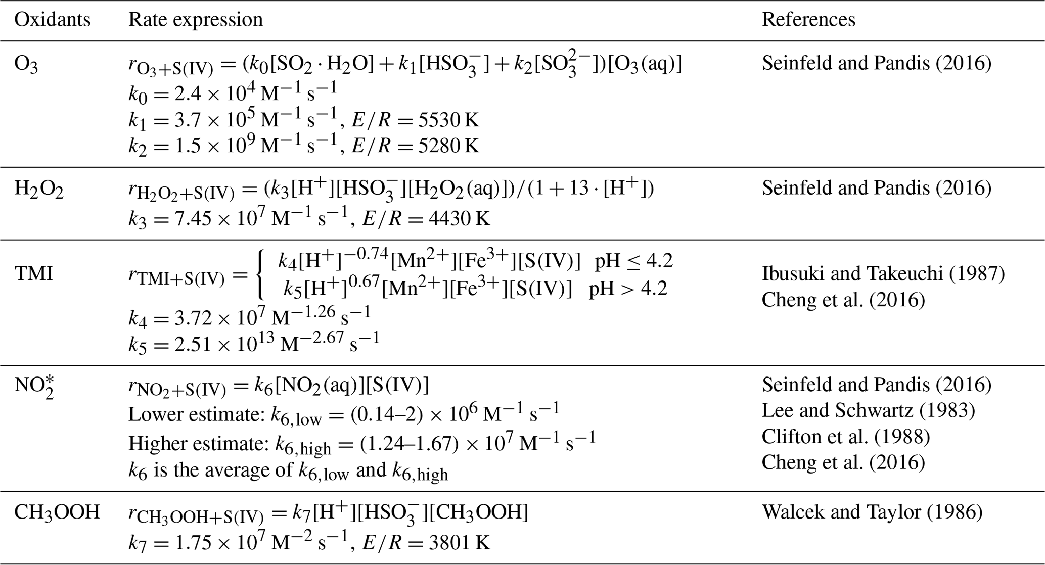
^* The rate coefficient k₆ (in M⁻¹ s⁻¹) is expressed as follows: $k_{\mathrm{6}}=\left\{\begin{array}{l}(k_{\mathrm{6},\mathrm{low},\mathrm{1}}+k_{\mathrm{6},\mathrm{high},\mathrm{1}})/\mathrm{2}\text{pH}\le \mathrm{5}\\ (k_{\mathrm{6},\mathrm{low},\mathrm{1}}+(\mathrm{pH}-\mathrm{5})/\mathrm{0.8}\times (k_{\mathrm{6},\mathrm{low},\mathrm{2}}-k_{\mathrm{6},\mathrm{low},\mathrm{1}})+k_{\mathrm{6},\mathrm{high},\mathrm{1}})/\mathrm{2}\mathrm{5}<\text{pH}\le \mathrm{5.3}\\ (k_{\mathrm{6},\mathrm{low},\mathrm{1}}+(\mathrm{pH}-\mathrm{5})/\mathrm{0.8}\times (k_{\mathrm{6},\mathrm{low},\mathrm{2}}-k_{\mathrm{6},\mathrm{low},\mathrm{1}})+k_{\mathrm{6},\mathrm{high},\mathrm{1}}+(\mathrm{pH}-\mathrm{5.3})/\mathrm{3.4}\times (k_{\mathrm{6},\mathrm{high},\mathrm{2}}-k_{\mathrm{6},\mathrm{high},\mathrm{1}}\left)\right)/\mathrm{2}\mathrm{5.3}<\text{pH}\le \mathrm{5.8}\\ (k_{\mathrm{6},\mathrm{low},\mathrm{2}}+(\mathrm{pH}-\mathrm{5.3})/\mathrm{3.4}\times (k_{\mathrm{6},\mathrm{high},\mathrm{2}}-k_{\mathrm{6},\mathrm{high},\mathrm{1}}\left)\right)/\mathrm{2}\mathrm{5.8}<\text{pH}\le \mathrm{8.7}\\ (k_{\mathrm{6},\mathrm{low},\mathrm{2}}+k_{\mathrm{6},\mathrm{high},\mathrm{2}})/\mathrm{2}\text{pH}>\mathrm{8.7}\end{array}\right.$,
where $k_{\mathrm{6},\mathrm{low},\mathrm{1}}=\mathrm{0.14}\times {\mathrm{10}}^{\mathrm{6}}$ M⁻¹ s⁻¹, $k_{\mathrm{6},\mathrm{low},\mathrm{2}}=\mathrm{2}\times {\mathrm{10}}^{\mathrm{6}}$ M⁻¹ s⁻¹, $k_{\mathrm{6},\mathrm{high},\mathrm{1}}=\mathrm{1.24}\times {\mathrm{10}}^{\mathrm{7}}$ M⁻¹ s⁻¹, $k_{\mathrm{6},\mathrm{high},\mathrm{2}}=\mathrm{1.67}\times {\mathrm{10}}^{\mathrm{7}}$ M⁻¹ s⁻¹.

Following B. Zheng et al. (2015) and Chen et al. (2016), a parameterization scheme is adopted to simulate the aqueous-phase production of nitrate (denoted as PM25_NO3):

$$\begin{array}{}\text{(2)}& \begin{array}{rl}& {\displaystyle \frac{\mathrm{d}{C}_{\mathrm{PM}\mathrm{25}\mathrm{\_}\mathrm{NO}\mathrm{3}}}{\mathrm{d}t}}={\left({\displaystyle \frac{R_{\mathrm{d}}}{D_{\mathrm{g},{\mathrm{NO}}_{\mathrm{2}}}}}+{\displaystyle \frac{\mathrm{0.04}}{{\mathit{\gamma }}_{{\mathrm{NO}}_{\mathrm{2}}}\sqrt{\mathrm{8}RT/\mathit{\pi }{M}_{\mathrm{w},{\mathrm{NO}}_{\mathrm{2}}}}}}\right)}^{-\mathrm{1}}\\ & \cdot \mathrm{Aa}\cdot C_{{\mathrm{NO}}_{\mathrm{2}}\left(\mathrm{g}\right)},\end{array}\end{array}$$

where Aa is the surface area concentration of fine particles (cm² cm⁻³) and γ is the uptake coefficient (unitless) for NO₂. The uptake coefficient γ has a lower limit ($\mathrm{3.0}\times {\mathrm{10}}^{-\mathrm{6}}$) and a higher limit ($\mathrm{13.0}\times {\mathrm{10}}^{-\mathrm{6}}$) when the relative humidity (RH) is lower than 50 % and higher than 90 %, respectively. Note that the γ has been scaled 15 times lower than that used in B. Zheng et al. (2015) to better match the observed PM25_NO3 with R=0.74 and NMB =3 % (normalized mean bias; see more details in Sect. 3.1). When the RH ranges between 50 % and 90 %, the value for γ is then linearly interpolated between the two limits.

To simulate aerosol water content (AWC) and pH as input parameters of the AWAC module, we have replaced the original ISORROPIA model in WRF-Chem with an improved version of ISORROPIA II (Fountoukis and Nenes, 2007; Song et al., 2018). The source code of the improved ISORROPIA II is available at http://wiki.seas.harvard.edu/geos-chem/index.php/ISORROPIA_II (last access: 6 October 2020). ISORROPIA predicts the thermodynamic equilibrium (including pH) for an internal-mixed system of multiple inorganic components at a specific temperature and humidity. Following Ding et al. (2019), we assume that the phase state for aerosol is metastable at RH >30 %; otherwise the phase state is stable. If the predicted AWC is less than an infinitesimal value (the threshold value of 10⁻⁸ µg m⁻³ is used; see Figs. S6 and S7 of Supplement for relevant uncertainties), pH is set to a missing value, and heterogeneous reactions in aerosol water are not calculated. Otherwise the heterogeneous oxidation module is called assuming a fixed number and/or size distribution and thermodynamic status (including AWC and pH) within one time step of the master chemistry module in WRF-Chem program.

The RACM mechanism (Stockwell et al., 1997, 1990) is used to calculate the gas-phase photochemistry and provides the concentrations of gaseous precursors (e.g., SO₂, NO₂, etc.) and oxidants (e.g., O₃, H₂O₂, etc.). The MADE/SORGAM scheme (Ackermann et al., 1998; Schell et al., 2001) with the improved ISORROPIA II model is used to simulate the aerosol dynamics (including nucleation, coagulation, and condensation) and thermodynamics and provide the aerosol's size distribution and number concentration, as well as AWC and pH values. The integrated process rate (IPR) technique (Tao et al., 2017, 2015) is used to record the formation rates of sulfuric and nitric acid vapor through photochemical oxidation in the gas phase.

For the TMI oxidation pathway, we assume that Fe³⁺ and Mn²⁺ will not be consumed in the TMI pathway due to the catalytic nature of ${\mathrm{Fe}}^{\mathrm{3}+}/{\mathrm{Mn}}^{\mathrm{2}+}$. The concentrations of Fe³⁺ and Mn²⁺ (in mol L⁻¹) in aerosol water can be calculated by Eq. (3):

$$\begin{array}{}\text{(3)}& \left\{\begin{array}{l}\left[{\mathrm{Fe}}^{\mathrm{3}+}\right]=\mathrm{Min}(C_{\mathrm{PM}\mathrm{25}\mathrm{\_}\mathrm{FE}}\cdot {\mathrm{FS}}_{\mathrm{FE}{\mathrm{3}}^{+}}/\mathrm{AWC},\\ \mathrm{2.6}\times {\mathrm{10}}^{-\mathrm{38}}/\left[{\mathrm{OH}}^{-}{]}^{\mathrm{3}}\right)\\ \left[{\mathrm{Mn}}^{\mathrm{2}+}\right]=\mathrm{Min}(C_{\mathrm{PM}\mathrm{25}\mathrm{\_}\mathrm{MN}}\cdot {\mathrm{FS}}_{\mathrm{MN}{\mathrm{2}}^{+}}/\mathrm{AWC},\\ \mathrm{1.6}\times {\mathrm{10}}^{-\mathrm{13}}/{[\mathrm{OH}}^{-}{]}^{\mathrm{2}})\end{array}\right.,\end{array}$$

where PM25_FE and PM25_MN are the fine particle components of Fe and Mn minerals, respectively, C denotes the concentrations in moles per liter of air, FS${}_{\mathrm{FE}{\mathrm{3}}^{+}}$ and FS${}_{\mathrm{MN}{\mathrm{2}}^{+}}$ represent the maximum fractional solubility of Fe³⁺ and Mn²⁺, respectively (regardless of the acidity of aerosol water), and AWC is the aerosol liquid water content in liters per liter of air.

2.2 WRF-Chem model configuration and scenarios

The modeling framework is constructed on a single domain of 100 (west–east) ×70 (south–north) ×30 (vertical layers) grid cells with a horizontal resolution of 20 km (including the Gobi Desert; see Fig. S8 of Supplement). The overview of the chemical and physical options used in this study is summarized in Table S6 of Supplement. The Madronich F-TUV photolysis scheme (Madronich, 1987) is used to calculate the photolysis rates. The initial and boundary conditions for meteorology and chemistry are derived from $\mathrm{1.0}{}^{\circ }\times \mathrm{1.0}{}^{\circ }$ National Center for Environmental Prediction Final (NCEP FNL) data and global-scale MOZART outputs, respectively. Observation nudging (Liu et al., 2005) is used to nudge the modeled temperature, wind fields, and humidity towards the observations (including surface and upper layers). The multi-resolution Emission Inventory for China (MEIC) of the year 2013 (Lei et al., 2011; Zhang et al., 2009; Li et al., 2014, 2017b) is used for anthropogenic emissions. The Megan scheme (Guenther et al., 2006) is used for biogenic volatile organic compound emissions. The hourly biomass burning emissions data are provided by the fire inventory from the National Center for Atmospheric Research (NCAR) (FINN; Wiedinmyer et al., 2011). We use the GOCART dust scheme (Ginoux et al., 2001; Zhao et al., 2010, 2013), which is coupled with the MADE/SORGAM aerosol scheme.

In this study, we have simulated 15 scenarios as detailed in Table 2, including an original (ORIG) scenario with WRF-Chem (original chemistry) and default emissions as mentioned above, a control (CTRL) scenario with WRF-Chem-AWAC (with implementation of aerosol water aqueous-phase chemistry) and optimized ammonia emission, as well as additional emissions for chloride and crustal fine particles, and 13 sensitivity scenarios with respect to the CTRL scenario. Since anthropogenic source chlorine is not included in MEIC, we adopt the chlorine inventory in Liu et al. (2018), which provides the emissions of HCl from coal consumption. WRF/Chem prescribes a specific mass ratio of the fine mode dust emission to the total dust emission, and we further adopt the fine mode dust emission speciation profiles from Dong et al. (2016). The mass fractions for fine particle components of K, Na, Ca, Mg, Fe, and Mn minerals (denoted as PM25_K, PM25_NA, PM25_CA, PM25_MG, PM25_FE, and PM25_MN, respectively) from dust sources are set as 3.77 %, 3.94 %, 7.94 %, 0.80 %, 2.43 %, and 0.063 %, respectively. Dry and wet depositions are also considered for these newly added crustal fine particle components, as detailed in Sect. S2.2 of Supplement.

Table 2 Description for different scenarios in this study.

The CTRL scenario is expected to reproduce the observed fine particle compositions (including sulfate, nitrate, ammonium, chloride, and crustal components) and gas-phase pollutants and thus more reliably predict the spatiotemporal distribution of pH, AWC, and sulfate production. For this purpose, five parameters in the CTRL scenario have been adjusted to better match the observations (with the criteria that the relative error of the monthly mean concentrations of different fine particle components is less than 5 %), namely the factor multiplied by the anthropogenic ammonia emissions (denoted as emissf${}_{{\mathrm{NH}}_{\mathrm{3}}}$), the factor multiplied by dust speciation fractions for PM25_K, PM25_NA, PM_CA and PM25_MG (denoted as emissf_OCAT), and the factor multiplied by the anthropogenic chloride emissions (denoted as emissf_CL), as well as FS${}_{\mathrm{FE}{\mathrm{3}}^{+}}$ and FS${}_{\mathrm{MN}{\mathrm{2}}^{+}}$ (the maximum fractional solubility of Fe³⁺ and Mn²⁺ in Eq. 3, respectively). In the CTRL scenario, emissf${}_{{\mathrm{NH}}_{\mathrm{3}}}$ has been set to 2 as recent studies using top-down inverse modeling (Van Damme et al., 2018; L. Zhang et al., 2018; Wang et al., 2018; Kong et al., 2019) and direct measurement (Wang et al., 2018) found that previous bottom-up inventories might underestimate the NH₃ emissions, and the MEIC inventory was estimated to underpredict NH₃ emissions by about 40 % over the North China Plain (Kong et al., 2019). As shown in Table S7 of the Supplement, compared to the scenario using the default MEIC emission data, the CTRL scenario (with doubled NH₃ emissions) better matches both the observed ammonia and ammonium concentrations at urban Beijing sites during wintertime (Meng et al., 2011; Liu et al., 2017; Song et al., 2018). To match the observations of PM25_OCAT, the emissf_OCAT is set to 4.5 (the total dust emission is unchanged) as Dong et al. (2016) indicated that observed fine particles should have a considerably higher mass contribution within the East Asian dust than the chemical transport model prescribes, and emissf_CL is set to 6 to match the observations of PM25_CL. To have a better agreement with the sulfate observation, FS${}_{\mathrm{FE}{\mathrm{3}}^{+}}$ and FS${}_{\mathrm{MN}{\mathrm{2}}^{+}}$ are set to 7 % and 40 %, respectively. Note that the assumption behind tuning only FS${}_{\mathrm{FE}{\mathrm{3}}^{+}}$ and FS${}_{\mathrm{MN}{\mathrm{2}}^{+}}$ to better agree with observed sulfates is that the model could reasonably simulate the concentrations of other oxidants (e.g., OH, H₂O₂, O₃, and NO₂); thus, the deviation from observation can be attributed to the uncertainties in representations of the TMI pathway. Note that uncertainties in the emission, transport (i.e., advection and turbulent mixing), removal (dry and wet deposition), and sulfate formation in other phases could also contribute to the discrepancies between modeling results and observations. Nonetheless, this study does not aim to estimate the exact values for aerosol pH and sulfate formation budget. Instead, this study focuses on investigating the characteristics of the spatiotemporal distribution of aerosol pH, as well as sulfate formation budget, and also the uncertainties relevant to assumptions for input parameters. Journet et al. (2008) found that the dust mineralogy was a critical factor for iron solubility, and fractional Fe solubility was observed to be ∼4 % and less than 1 % for samples of clay and iron (hydr-)oxides, respectively. A low fractional Fe solubility approximately or below 0.05 % was reported for the non-atmospherically processed arid soil samples (Schroth et al., 2009; Johnson et al., 2010; Shi et al., 2012). Most of the Fe minerals exist in the form of hematite (α-Fe₂O₃) over the Gobi Desert (Claquin et al., 1999), and fractional Fe solubility was increased to 1 %–2 % after 3–5 d transport from the Gobi Desert (Meskhidze et al., 2003). A higher fractional Fe solubility up to ∼10 % was reported after a longer time of atmospheric aging for dust particles (Takahashi et al., 2011; Shi et al., 2012). Fractional Mn solubility for dust particles was observed to range between 20 % and 60 % (Duvall et al., 2008; Baker et al., 2006; Hsu et al., 2010). The rest of the 13 scenarios are used for sensitivity analyses on the uncertainties in emissf${}_{{\mathrm{NH}}_{\mathrm{3}}}$, emissf_OCAT, emissf_CL, FS${}_{\mathrm{FE}{\mathrm{3}}^{+}}$, and FS${}_{\mathrm{MN}{\mathrm{2}}^{+}}$, as well as phase state assumption.

3 Results and discussion

3.1 Comparison of CTRL and ORIG scenarios

Figure 1 shows the comparison of ORIG and CTRL scenarios against observations obtained at the site located on the campus of Tsinghua University in Beijing (denoted as the Beijing TSU site; $\mathrm{40}{}^{\circ }{\mathrm{00}}^{\prime }{\mathrm{17}}^{\prime \prime }$ N, $\mathrm{116}{}^{\circ }{\mathrm{19}}^{\prime }{\mathrm{34}}^{\prime \prime }$ E, ∼10 m height) during January 2013. The hourly data include online observations of concentrations of SO₂, PM25_SO4, NO_x (= NO + NO₂), PM25_NO3, O₃, and PM_2.5, as well as relative humidity (RH) that is closely related to the AWC. Details about the measurements have been described in G. J. Zheng et al. (2015) and Cheng et al. (2016). As shown in Fig. 1, simulations from both scenarios were capable of reproducing the concentration levels of the sum of SO₂ and PM25_SO4, the sum of NO_x and PM25_NO3, O₃, and PM_2.5 with the normalized mean bias (NMB) around ±30 % and the correlation coefficients (R) ranging between 0.5 and 0.7. The simulated RH matched the observations well with an NMB of ∼12 % and an R of ∼0.9. Simulations of PM25_SO4 and PM25_NO3 have been significantly improved in the CTRL scenario.

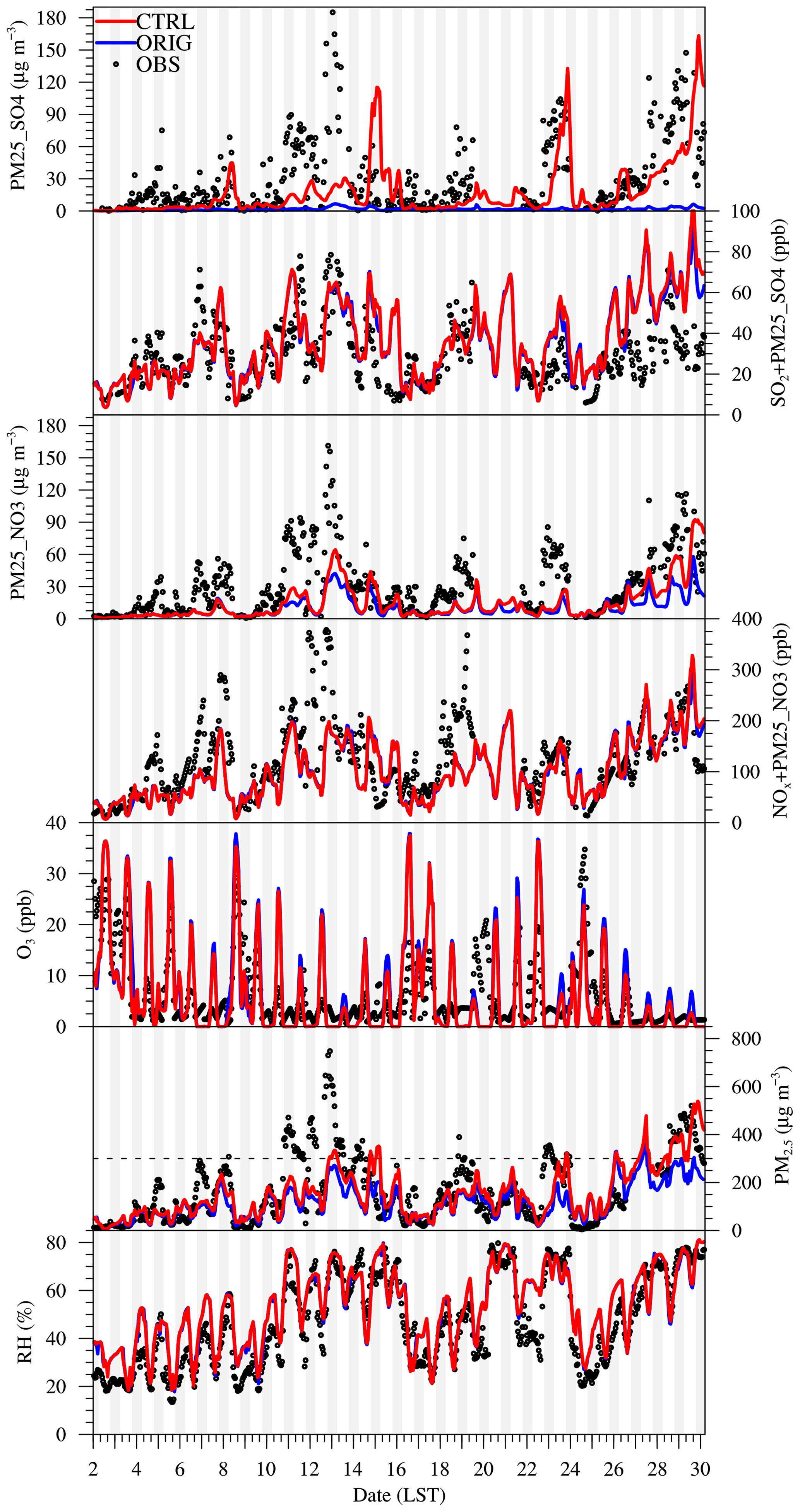
Figure 1 Comparison of hourly model results and observations (OBS) for ORIG and CTRL scenarios at the Beijing TSU site during January 2013. The compared parameters include modeled hourly concentrations of fine particulate sulfate (PM25_SO4), the sum of SO₂ and PM25_SO4 (PM25_SO4 converted to the equivalent volume mixing ratio of SO₂), fine particulate nitrate (PM25_NO3), the sum of NO_x and PM25_NO3 (PM25_NO3 converted to the equivalent volume mixing ratio of NO_x), O₃, and PM_2.5, as well as hourly relative humidity (RH).

Offline observations of PM25_K, PM25_NA, PM25_CA, PM25_MG, PM25_CL, PM25_SO4, PM25_NO3, and PM25_NH4 are also available on a daily basis (G. J. Zheng et al., 2015; Cheng et al., 2016). As shown in Fig. 2, simulations of sulfate, nitrate, and ammonium in PM_2.5 were greatly improved in the CTRL scenario with an NMB within ±5 %, while the NMB of the ORIG scenario was −90 % for sulfate, −35 % for nitrate, and −65 % for ammonium. The only source of PM25_CL in the ORIG scenario was sea salt emissions, and it was negligible. The improved model WRF-Chem-AWAC with additional chloride emissions from coal combustion could capture the observed PM25_CL with an NMB of only ∼10 %. Other inorganic cations in PM_2.5 (denoted as PM25_OCAT and only involving PM25_K, PM25_NA, PM25_CA, and PM25_MG) were not included in the original MADE/SORGAM scheme, and thus their concentrations were zero in the ORIG scenario. The CTRL scenario could moderately reproduce the concentrations of PM25_OCAT with an NMB of ∼60 %. Note that the emission of PM25_OCAT has been adjusted based on the criteria of reducing the mismatch of simulation and observation within 5 % on a monthly mean basis, and here the NMB was calculated based on daily values.

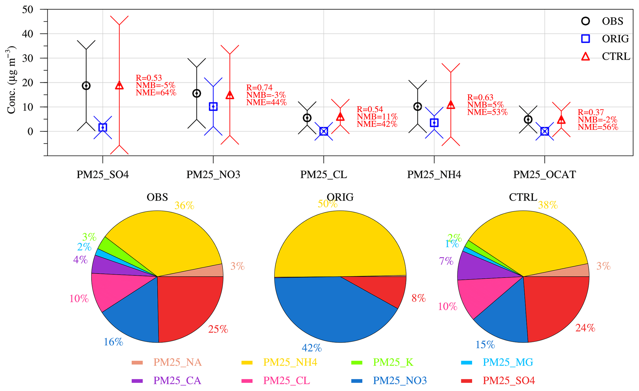
Figure 2 The significant improvement of simulations in the CTRL scenario compared to the ORIG scenario. Bottom panel: observed (OBS) and simulated (scenarios of ORIG and CTRL) mean electric charge fractions for fine particulate sulfate (PM25_SO4, using ${\mathrm{SO}}_{\mathrm{4}}^{\mathrm{2}-}$ as the surrogate), nitrate (PM25_NO3), ammonium (PM25_NH4), chloride (PM25_CL), sodium (PM25_NA), potassium (PM25_K), calcium (PM25_CA), and magnesium (PM25_MG) at the Beijing TSU site during January 2013. Top panel: observed (OBS) and simulated (scenarios of ORIG and CTRL) concentrations (both average and standard deviation are shown) for fine particulate sulfate (PM25_SO4), nitrate (PM25_NO3), chloride (PM25_CL), ammonium (PM25_NH4) and other cation components (PM25_OCAT = PM25_NA + PM25_K + PM25_CA + PM25_MG) at the Beijing TSU site during January 2013.

As shown in the lower panels of Fig. 2, among the fine particle components mentioned above, observed PM25_NH4 and PM25_OCAT accounted for about 75 % and 25 % of the monthly mean ionic charge budget for cations, respectively. Observed PM25_CL, PM25_NO3, and PM25_SO4 accounted for about 20 %, 32 %, and 48 % of the monthly mean ionic charge budget for anions, respectively. The CTRL scenario could capture well the observed ionic charge budget except that the mole fraction of PM25_CA in PM25_OCAT was slightly overestimated (PM25_CA had a higher mass fraction for dust emission speciation). Thus, in the following sections, the CTRL configuration is used to study the temporal and spatial distribution of aerosol pH and the regime transition of sulfate formation in aerosol water during winter haze events in the North China Plain.

3.2 Vertical profile of pH over Beijing

Figure 3a shows the vertical profile of the simulated aerosol pH over the Beijing site. The mean pH at the surface layer was ∼5.4 (daytime mean pH ∼5.2 and nighttime mean pH ∼5.6), and it remained nearly constant around ∼5 up to ∼2 km above ground level (a.g.l.), while above ∼2 km a.g.l., the mean pH exhibited a more rapid decrease and became highly acidic (mean pH ∼0) at ∼3 km a.g.l. Based on observations of aerosol compositions, Guo et al. (2016) also reported that pH at the middle troposphere of 5 km a.g.l. was highly acidic (mean pH $\sim -\mathrm{0.7}$) and was about 1.7 units lower than at the surface layer over the northeastern Unites States. These spatial features for pH were closely associated with the spatiotemporal variation in the abundance of acidic and alkaline fine particle components and their gaseous counterparts. Here, the acidic fine particle components include total sulfate (SO4^T = H₂SO₄(g) + PM25_SO4), total nitrate (NO3^T = HNO₃(g) + PM25_NO3), and total chloride (Cl^T = HCl(g) + PM25_CL), and the alkaline components include total ammonia (NH_x = NH₃(g) + PM25_NH4) and PM25_OCAT.

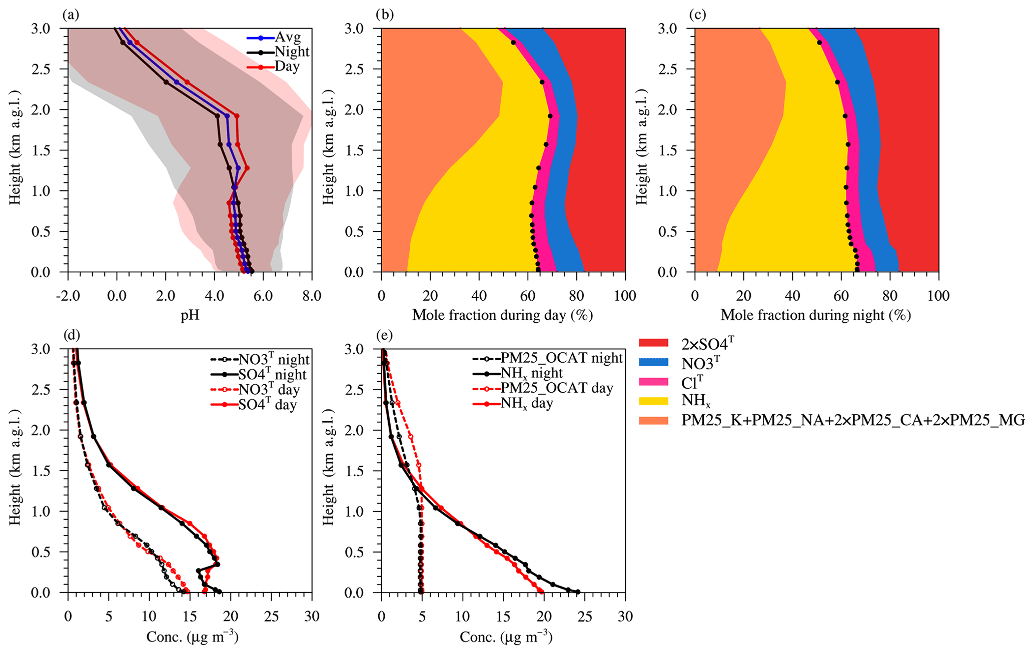
Figure 3 Vertical profiles of the fine particle pH and its potential influencing factors over the Beijing TSU site. The data are simulated with the CTRL scenario during January 2013 and presented at height above ground level (a.g.l.). (a) Monthly average pH (blue), as well as daytime (red) and nighttime (black) average pH (standard deviations are shown in light red and light gray shading, respectively). (b) Daytime mole fractions for the electric charge of total ammonia (NH_x), total chloride (Cl^T), total sulfate (SO4^T), total nitrate (NO3^T), and different crustal components of PM_2.5, and the black dots represent the vertical profile of cation^T ∕ (cation^T+ anion^T). (c) The same as in (b) but for the nighttime. (d) Daytime (red) and nighttime (black) concentrations of total sulfate (SO4^T) and total nitrate (NO3^T). (e) Daytime (red) and nighttime (black) concentrations of NH_x and PM25_OCAT.

Thus, we define the concentrations of total potential anion (anion^T) and total potential cation (cation^T) as follows:

$$\begin{array}{}\text{(4)}& {\displaystyle }{C}_{{\mathrm{anion}}^{\mathrm{T}}}=\mathrm{2}\cdot C_{{\mathrm{SO}\mathrm{4}}^{\mathrm{T}}}+C_{{\mathrm{NO}\mathrm{3}}^{\mathrm{T}}}+C_{{\mathrm{Cl}}^{\mathrm{T}}},\text{(5)}& {\displaystyle }\begin{array}{rl}{C}_{{\mathrm{cation}}^{\mathrm{T}}}=& C_{{\mathrm{NH}}_{\mathrm{x}}}+C_{\mathrm{PM}\mathrm{25}\mathrm{\_}\mathrm{NA}}+C_{\mathrm{PM}\mathrm{25}\mathrm{\_}\mathrm{K}}\\ & +\mathrm{2}\cdot C_{\mathrm{PM}\mathrm{25}\mathrm{\_}\mathrm{MG}}+\mathrm{2}\cdot C_{\mathrm{PM}\mathrm{25}\mathrm{\_}\mathrm{CA}}.\end{array}\end{array}$$

As shown in Fig. 3b–c, the concentration ratio of cation^T to anion^T slightly changed (consistently decreased with increasing height at nighttime but firstly decreased and then increased with the increasing height in daytime) below ∼2 km a.g.l. and rapidly decreased above ∼2 km a.g.l. NH_x had the predominant mole fraction in the sum of anion^T and cation^T below the lower free troposphere (below ∼1 km a.g.l.), but its concentrations decreased sharply with the increasing height (Fig. 3e) as ammonia only had surface emissions. Although also dominated by the surface emission source of SO₂ and NO_x, both SO4^T (= H₂SO₄(g) + PM25_SO4) and NO3^T (= HNO₃(g) + PM25_NO3) could be produced through different gas-phase and aqueous-phase oxidation pathways at different altitudes. Thus, although their concentrations also decreased with the increasing altitude (Fig. 3d), the decreasing rate was slower than that of NH_x (Fig. 3d–e), which led to an increase in the mole fraction of anion^T above ∼2 km a.g.l. (Fig. 3b–c). The vertical profile of PM25_OCAT was distinct from that of NH_x (Fig. 3e), with its concentrations remaining almost constant until ∼1.5 km a.g.l. and decreasing relatively slowly above it, suggesting a different source possibly from high-altitude transport. Based on satellite, lidar, and surface measurement data, Huang et al. (2008) studied the vertical structure of Asian dust originating from the Taklamakan and Gobi deserts and found that dust particles could be uplifted to an altitude of ∼9 km around the source region, followed by the efficient eastward transport mainly via westerly jets. X.-X. Zhang et al. (2018) also investigated the dust layering structure over some cities in East Asia (including Beijing, Seoul, and Tokyo) and indicated that the dust particles were mixed well in the boundary layer before the intensive intermingling of subsiding layers from above (the passage of a dust storm). Our simulation also shows that PM25_OCAT over the Beijing site was evenly mixed after a long-range transport from its source region (mainly in the Gobi Desert; shown in Fig. S9 of the Supplement) below the lower free troposphere. Under different environmental conditions, the changes in concentrations and mole fractions of acidic and alkaline components could lead to competition and different dominant factors in the changes of pH vertically. Above ∼2 km, the influences of acidic components (mainly SO4^T and NO3^T) on pH eventually prevailed over those of alkaline components. Interestingly, PM25_OCAT could play a key role in maintaining a less acidic pH at ∼1.5–2.0 km a.g.l. A sensitivity test shows that if the PM25_OCAT is completely removed (in OCAT0 scenario), pH at 2.0 km a.g.l. would be ∼1 unit lower (more acidic) than that at 1.5 km a.g.l.

3.3 Diurnal cycle of pH over Beijing

Figure 3a shows that at the Beijing site, the nighttime pH was slightly higher than the daytime pH below ∼1 km a.g.l. but became lower above ∼1 km. As shown in Fig. 4, such an opposite pattern was largely driven by a different diurnal cycle of aerosol pH at different altitudes. Aerosol pH at the surface layer showed a minimum in the early afternoon, while at 2 km it showed a maximum around this time (Fig. 4a–b). The diurnal variation of pH also showed a highly similar pattern as the mole ratio of cation^T to anion^T (Fig. 4a–b). At the surface layer, concentrations of cation^T were considerably higher than concentrations of anion^T (Fig. 4d); furthermore, the diurnal variation of NH_x to a large extent explained the diurnal cycle pattern of cation^T. Daytime NH_x concentrations were significantly lower than at nighttime due to stronger boundary layer mixing. Following Song et al. (2018), we define the concentrations of required NH_x (${\mathrm{NH}}_x^{\mathrm{Req}}$) as follows:

$$\begin{array}{}\text{(6)}& \begin{array}{rl}{C}_{{\mathrm{NH}}_x^{\mathrm{Req}}}=& \mathrm{2}\cdot C_{\mathrm{SO}{\mathrm{4}}^{\mathrm{T}}}+C_{\mathrm{NO}{\mathrm{3}}^{\mathrm{T}}}+C_{{\mathrm{Cl}}^{\mathrm{T}}}-C_{\mathrm{PM}\mathrm{25}\mathrm{\_}\mathrm{NA}}\\ & -C_{\mathrm{PM}\mathrm{25}\mathrm{\_}\mathrm{K}}-\mathrm{2}\cdot C_{\mathrm{PM}\mathrm{25}\mathrm{\_}\mathrm{MG}}-\mathrm{2}\cdot C_{\mathrm{PM}\mathrm{25}\mathrm{\_}\mathrm{CA}}.\end{array}\end{array}$$

The physical meaning of ${\mathrm{NH}}_x^{\mathrm{Req}}$ is that the minimum NH_x ideally immobilizes all the gas-phase H₂SO₄, HNO₃ and HCl. Thus, the concentration ratio of ${\mathrm{NH}}_x^{\mathrm{Req}}$ to NH_x describes the levels of ammonia excess (Liu et al., 2017; Song et al., 2018). The diurnal cycles of pH and ammonia excess matched quite well with each other (Fig. 4b), and enhanced ammonia excess corresponded with a higher pH during nighttime. PM25_OCAT (mainly originating from long-range transport) concentrations were higher in daytime. SO4^T rapidly accumulated during the night (when the aqueous-phase production was active), while NO3^T concentrations reached their peak in the late afternoon (gas-phase oxidation played a more important role). As shown in Fig. 4c, a higher aerosol water content during nighttime (due to higher RH and PM_2.5 loading) would also contribute to the less acidic condition (G. J. Zheng et al., 2020). At the layer of ∼2 km a.g.l., the pH diurnal cycle was also similarly associated with the variation in the mole ratio of cation^T to anion^T (peaks around noon), and the diurnal variation of PM25_OCAT might play an important role.

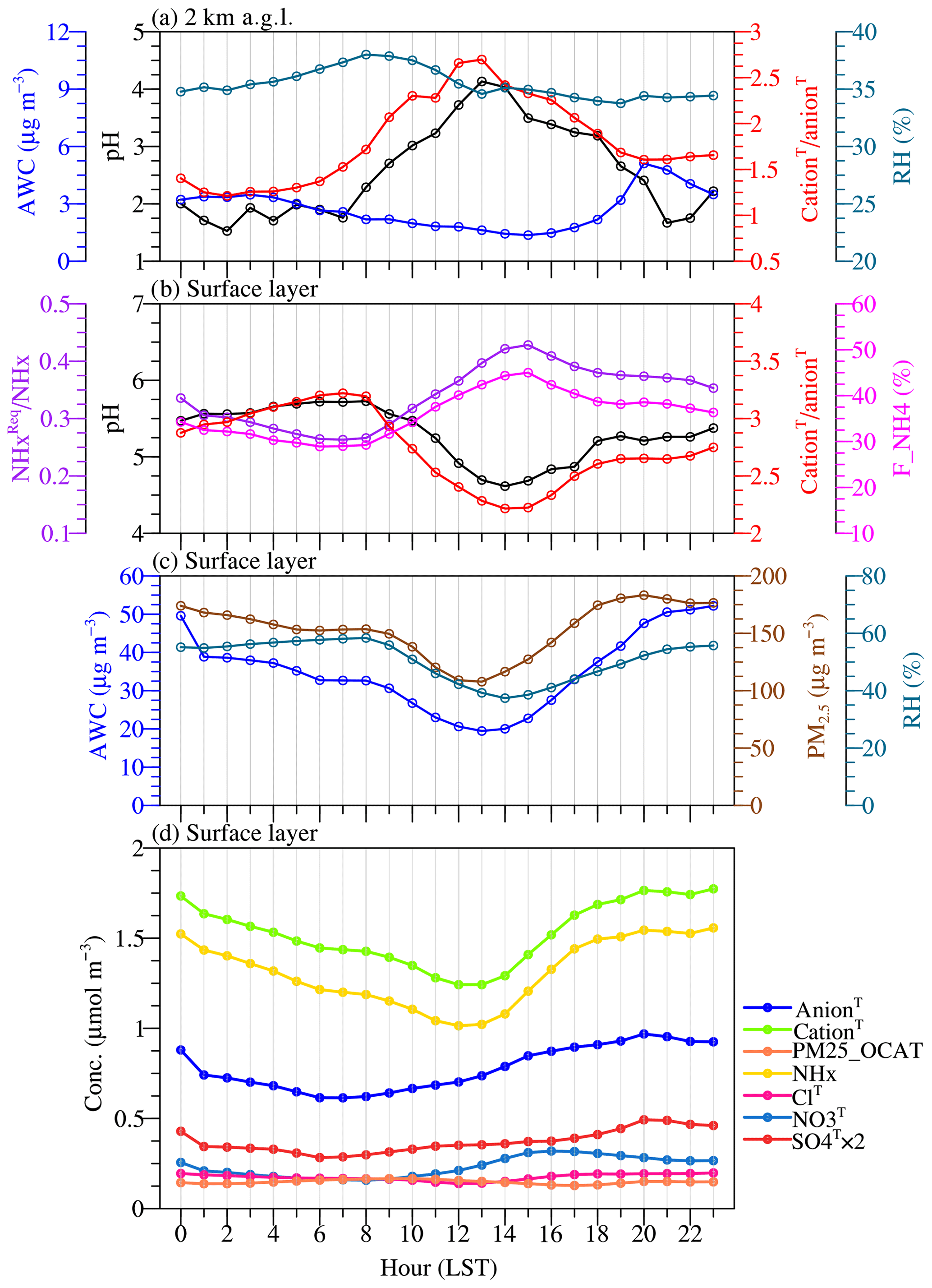
Figure 4 Monthly mean diurnal cycle for (a) fine particle pH, aerosol liquid water content (AWC), the mole ratio of total potential cation (cation^T) to total potential anion (anion^T), and relative humidity (RH) at 2 km a.g.l., (b) fine particle pH, the mole ratio of cation^T to anion^T, the mole ratio of required NH_x (${\mathrm{NH}}_x^{\mathrm{Req}}$) to NH_x, and fraction of NH_x in the particle phase (F_NH4) at the surface layer, (c) AWC, RH, and PM_2.5 concentrations at the surface layer, and (d) concentrations of total sulfate (SO4^T), total nitrate (NO3^T), total chloride (Cl^T), total ammonia (NH_x), PM25_OCAT, cation^T, and anion^T at the surface layer simulated in the CTRL scenario at the Beijing TSU site during January 2013.

3.4 Variabilities of pH over the North China Plain

Figure 5a–b show that aerosol pH at the surface layer exhibited a large spatial variability in the North China Plain. High pH greater than 6 was found in areas north of ∼41^∘ N, which could be attributed to abundant crustal components originating from dust and low concentrations of other aerosol inorganic compositions due to low emissions of precursors (e.g., SO₂, NO_x, and NH₃). In areas south of ∼41^∘ N, mean aerosol pH fell mostly between 4.4 and 5.7 (10 % and 90 % quantiles, respectively) with less contribution from crustal components. Mean pH over the sea mainly ranged between 4.0 and 4.5, generally lower than over most terrestrial areas. These marine and terrestrial areas with a relatively more acidic aerosol phase (pH ∼4.0 to 5.0) corresponded well with the spatial distribution of low NH_x zones (Fig. 5d). Moreover, a large temporal variability of pH was also found at the surface layer (Fig. 5c). The simulated standard deviation of pH mostly ranged between 0.4 and 2 and was higher over the northern areas with episodic dust events, as well as the southern areas with lower NH_x emissions.

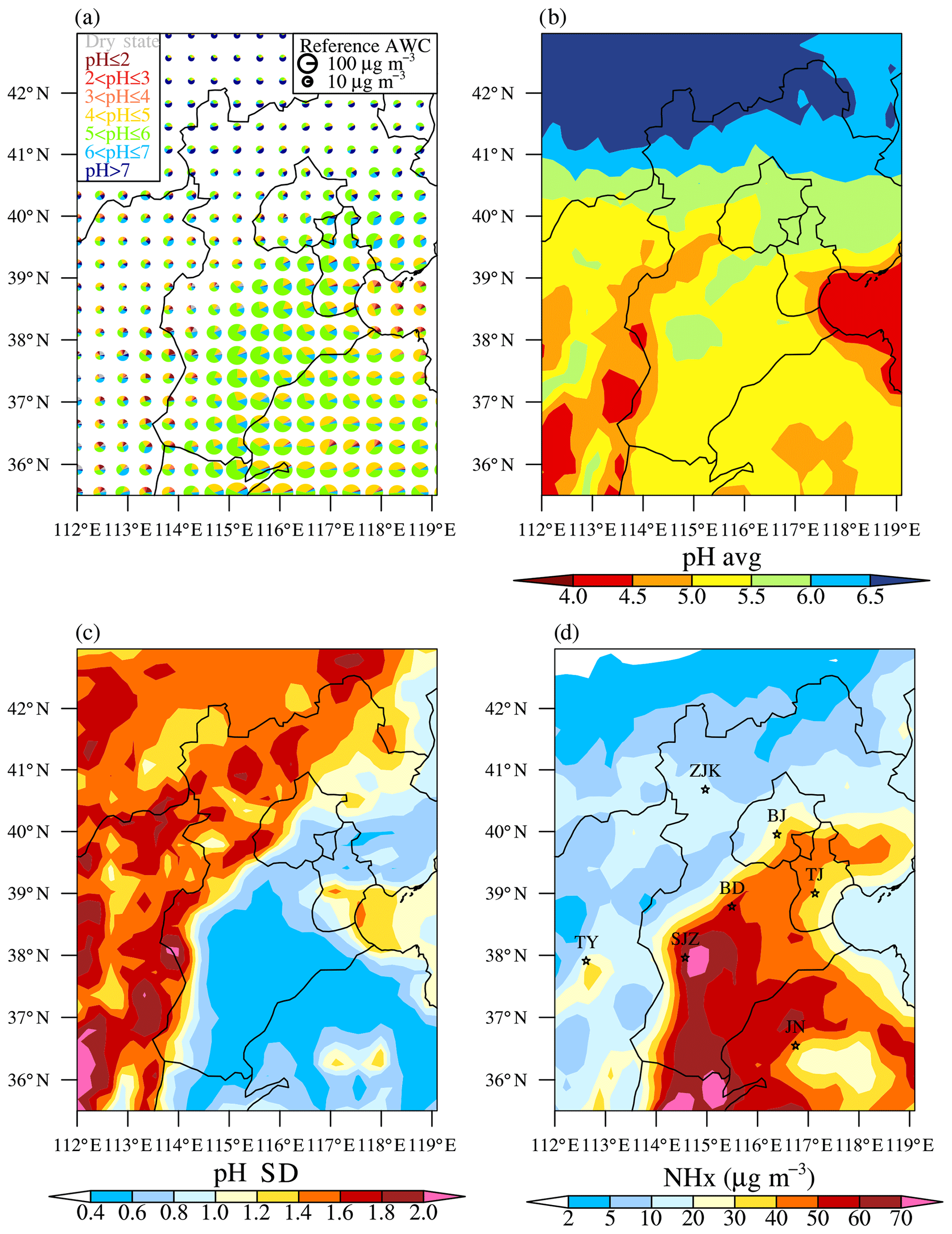
Figure 5 Fine particle pH and NH_x concentrations at the surface layer simulated in the CTRL scenario during January 2013. (a) The frequencies for different pH ranges. The radius R for the pie chart is scaled using $R/R_{\mathrm{ref}}=\mathrm{2}\exp \left(\log \mathrm{10}\right({\mathrm{AWC}/\mathrm{AWC}}_{\mathrm{ref}}\left)\right)$, and the reference radius R_ref and aerosol liquid water content (AWC_ref) are also shown. (b) The horizontal distribution of the average, (c) standard deviation for pH, and (d) the concentrations of NH_x. The locations for the seven cities of Beijing (BJ), Tianjin (TJ), Zhangjiakou (ZJK), Baoding (BD), Shijiazhuang (SJZ), Taiyuan (TY), and Jinan (JN) are also shown.

Figure 6a shows the latitude–height cross section of aerosol pH in the North China Plain. The trend that aerosol acidity was enhanced with increasing altitude was consistent for all the latitudes investigated. Nonetheless, the vertical gradients of pH varied among different locations and were closely associated with the vertical profile of the relative abundance of cation^T and anion^T, as well as air temperature and humidity (Fig. S10 of Supplement). Figure 6b further compares the vertical profiles of aerosol pH over seven different cities in the North China Plain (locations shown in Fig. 5c). The vertical profile pattern of aerosol pH was highly similar among Beijing, Tianjin, Baoding, and Shijiazhuang, for which the pH changed slightly until above ∼2 km a.g.l. However, as shown in Figs. 5c and S10, pH decreased rapidly from 1 to 2 km a.g.l. over both Zhangjiakou and Taiyuan maybe due to the lack of alkaline fine particle components (NH_x or PM25_OCAT). The rapid production of sulfate and nitrate at 0.5–1 km a.g.l. over Jinan was observed (Fig. S10), leading to a lower pH there. Furthermore, monthly mean nighttime pH was mostly higher than daytime pH in the lowest boundary layer below ∼100 m a.g.l.; however, no consistent pattern was found for the diurnal cycle pattern of pH in the upper tropospheric layers (Fig. 6c).

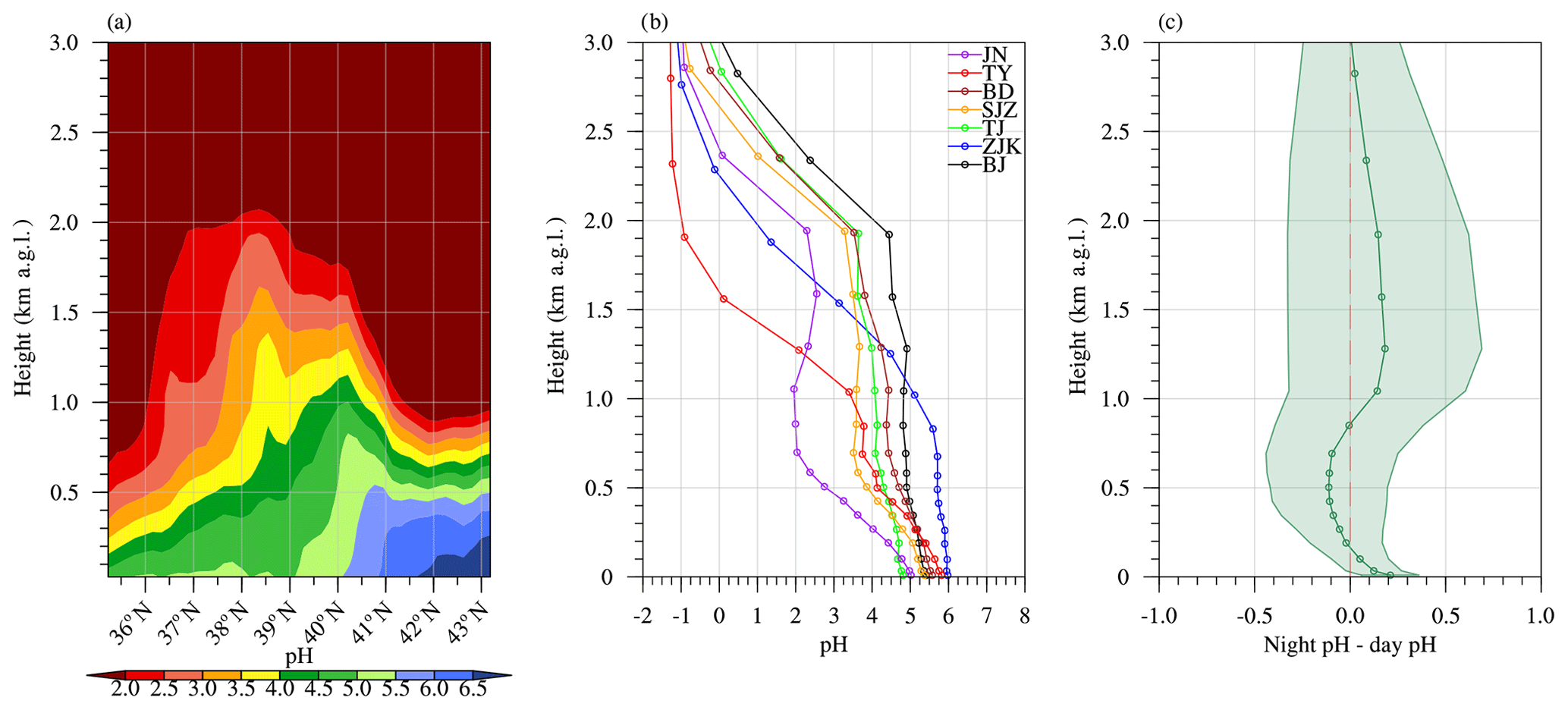
Figure 6 (a) Latitude–height cross section for the monthly mean fine particle pH averaged between 113 and 119^∘ E, (b) vertical profile for the monthly mean fine particle pH over the seven cities of Beijing (BJ), Tianjin (TJ), Zhangjiakou (ZJK), Baoding (BD), Shijiazhuang (SJZ), Taiyuan (TY), and Jinan (JN) (locations shown in Fig. 5c), and (c) vertical profile for the monthly mean day–night difference of pH (standard deviation is shown as shading) for the domain-wide grid cells in the CTRL scenario during January 2013.

3.5 Regime transition of sulfate formation

Figure 7a shows the averaged contribution of six sulfate formation pathways, namely aerosol water-phase oxidation by dissolved O₃, NO₂, H₂O₂, TMI (in the presence of O₂), and CH₃OOH, as well as gas-particle partitioning of H₂SO₄ vapor (GPP) at the surface layer. Note that H₂SO₄ vapor is produced mainly from the oxidation of SO₂ by OH radical and then partitions almost completely into the aerosol phase. For areas north of 41^∘ N, oxidation by dissolved O₃ was the most important pathway, followed by the TMI pathway. To the south of 41^∘ N, NO₂, TMI, and H₂O₂ pathways played the dominant role. The NO₂ reaction pathway prevailed in the megacity region of Beijing and the large area of Hebei Province to the south and west of Beijing, as well as part of Shandong Province, while the TMI pathway dominated in the inland region to the west and the coastal regions to the east of Beijing, and the H₂O₂ pathway dominated in the region further south in Shandong and Henan provinces. The regime transition of sulfate formation pathways were highly dependent on the spatial distribution of pH and oxidants and catalysts. As shown in Fig. 7b–e, the spatial distribution for O₃ exhibited an opposite pattern as NO_x; i.e., O₃ concentrations in urbanized areas (e.g., Beijing) with high NO_x emissions were considerably lower than less industrialized areas due to the titration effects of NO.

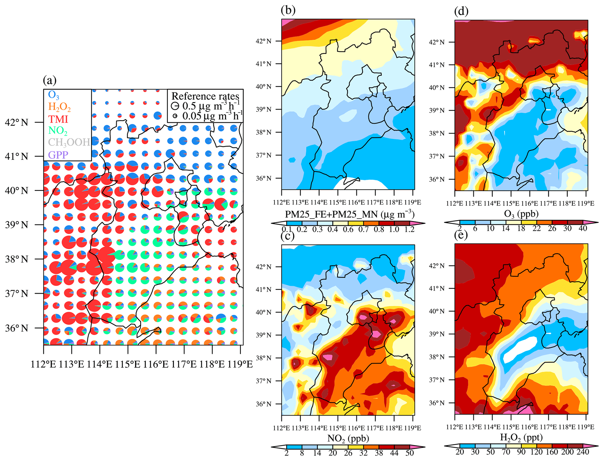
Figure 7 (a) The relative contributions of six sulfate formation pathways, namely aqueous-phase oxidation by dissolved O₃, H₂O₂, TMI (in presence of O₂), NO₂, and CH₃OOH, as well as gas-particle partitioning of H₂SO₄ vapor (GPP) at the surface layer simulated in the CTRL scenario during January 2013. The radius R for the pie chart in (a) is scaled using $R/R_{\mathrm{ref}}=\mathrm{2}\exp \left(\log \mathrm{10}\right(P/P_{\mathrm{ref}}\left)\right)$, and the reference sulfate production rate P is also shown. Horizontal distribution of the concentrations of (b) the sum of PM25_FE and PM25_MN, (c) NO₂, (d) O₃, and (e) H₂O₂ simulated in the CTRL scenario during January 2013.

Figure 8b shows the vertical profile of sulfate production rates averaged over the four dominant sulfate formation regimes at the surface layer (i.e., O₃, NO₂, TMI, and H₂O₂; shown in Fig. 8a). Consistent with the surface layer, the vertical regime transition of sulfate formation was highly dependent on the vertical distribution of pH and oxidants and catalysts (Fig. 8c–f). Both O₃ and TMI pathways played the dominant role at higher altitudes between 0.5 and 2.0 km a.g.l. (Fig. 8b). Interestingly, the vertical profile pattern for pH potentially enhanced the TMI pathway but hindered the O₃ pathway, while the vertical profile pattern for concentrations of oxidants and catalysts disfavored the TMI pathway but favored the O₃ pathway. As shown in Fig. 8b, the relative contributions of the NO₂ pathway rapidly decreased with increasing altitude, which is consistent with the decreasing trend in both NO₂ concentrations (Fig. 8f) and aerosol pH. The H₂O₂ pathway was non-negligible only in the lower boundary layer over the H₂O₂ regime and NO₂ regime. The GPP pathway tended to become more important with increasing altitude mainly due to the decreasing trend in aerosol water content. At higher altitudes above ∼3 km a.g.l., aqueous-phase oxidation in aerosol water became negligible.

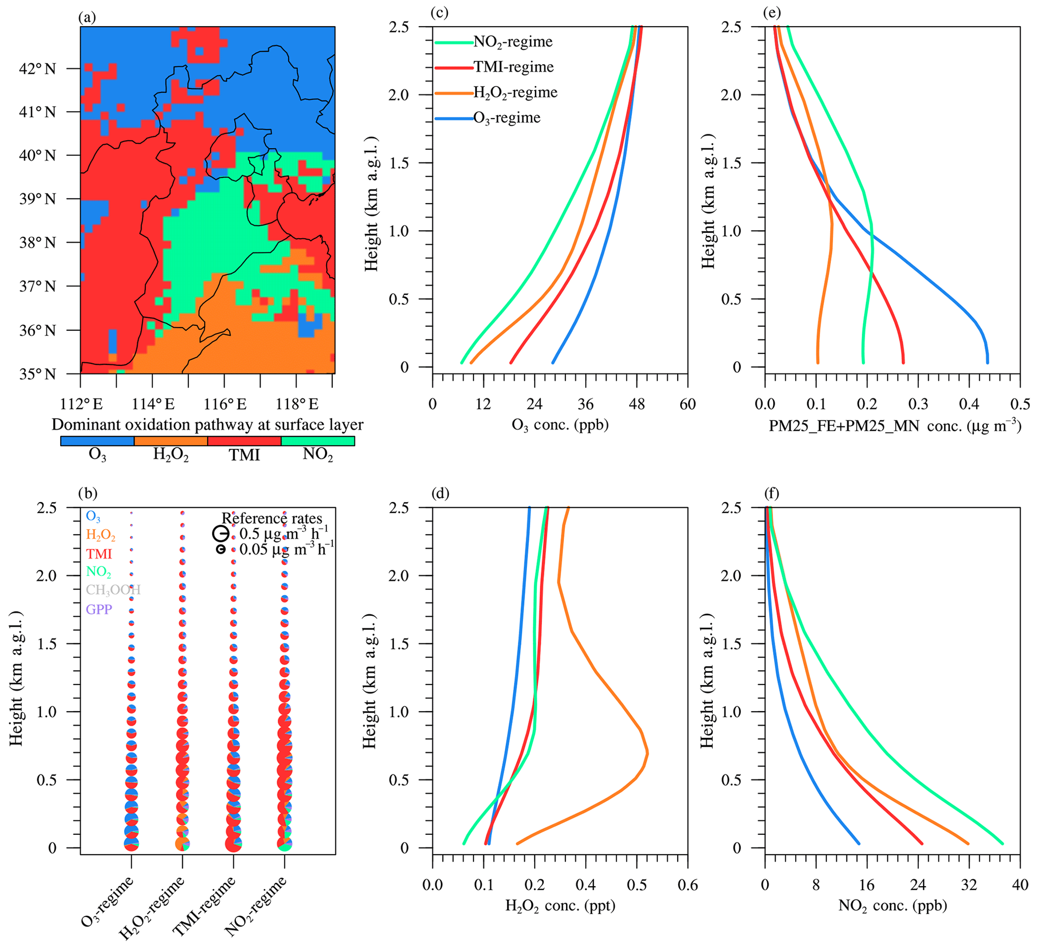
Figure 8 Dominant sulfate formation pathway at the surface layer (a) and the vertical profile of sulfate production through different pathways (b), as well as concentrations of the oxidants of O₃ (c), H₂O₂ (d), TMI (e), and NO₂ (f) averaged over the four dominant oxidation regimes (O₃, H₂O₂, TMI, and NO₂, respectively, as shown in Fig. 8a) and simulated in the CTRL scenario during January 2013. Contributions from different sulfate formation pathways are also shown in pie charts, and the radius R for the pie chart is scaled depending on the sulfate production rate P using $R/R_{\mathrm{ref}}=\mathrm{2}\exp \left(\log \mathrm{10}\right(P/P_{\mathrm{ref}}\left)\right)$.

Compared to nitrate, aqueous-phase oxidation was more important to sulfate formation in the North China Plain. For example, according to our simulation, over the Beijing site, below ∼2 km a.g.l., aqueous-phase oxidation in aerosol water accounted for ∼100 % and 80 %–90 % of SO4^T formation during nighttime and daytime, respectively. While, its respective contributions to nighttime and daytime NO3^T formation were only 40 %–70 % and 0 %–10 %.

3.6 Discussion

The uncertainties of predicted pH and sulfate formation relevant to the adjusted emission parameters (for NH₃, crustal minerals, Fe³⁺/Mn²⁺ ions, and chlorides) and assumed phase state are further investigated. We focus on four aspects, namely surface layer pH (denoted as pH_surf) and its day/night difference (denoted as ΔpH_{surf,night-day}), the difference between surface layer pH and pH at ∼2 km a.g.l. (denoted as ΔpH_surf-2 km), and surface layer sulfate production rates (denoted as P_S(VI),surf) through different pathways for the domain-wide grid cells south of 41^∘ N. As shown in Fig. 9, different scenarios predict different pH_surf and P_S(VI),surf; nonetheless, ΔpH_{surf,night-day} and ΔpH_surf-2 km are approximately 0.2 and 5.0, respectively, for almost all the sensitivity tests, indicating that the diurnal cycle pattern at the surface layer and the altitudinal decrease in pH will be robust.

We first examine the sensitivities of our results to NH₃ and crustal minerals. When NH₃ emissions are completely removed (A0 scenario), a strong acidic aerosol phase is predicted (mean pH_surf ∼0), while the P_S(VI),surf decreases by ∼60 % as in the CTRL scenario (due to lack of efficient water-absorbing ammoniates). If PM25_OCAT emissions are removed or halved (OCAT0 and OCAT0.5 scenarios), the averaged pH decreases to 4.2 and 4.6, respectively, and P_S(VI),surf increases by ∼250 % and ∼200 %, respectively, compared to the CTRL scenario (a lower pH favors sulfate production through the TMI pathway). Doubling both NH₃ and PM25_OCAT emissions (A2 and OCAT2 scenarios) leads to a slightly higher pH_surf and a similar P_S(VI),surf, with the sulfate formation dominated by NO₂ and O₃ pathways. For the control experiments of MEIC_CTRL (using the original MEIC inventory), predicted pH_surf is lower, and the relative contribution to sulfate formation is decreased for the NO₂ pathway but increased for the TMI pathway. Interestingly, rapid production of sulfate could be maintained over a wide pH range (∼4.2–5.7) with the varying emissions for NH₃ and crustal particles (transition between the dominant TMI pathway and dominant NO₂∕O₃ pathway).

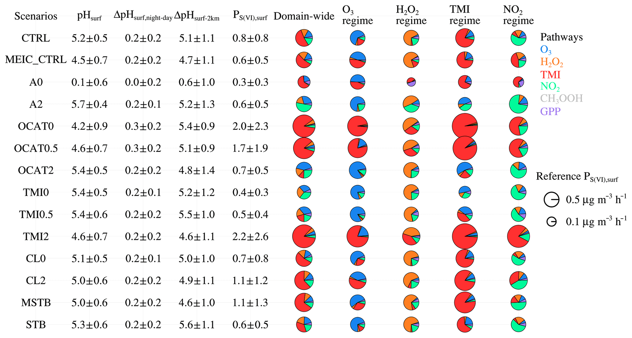
Figure 9 Surface layer pH (denoted as pH_surf) and its day–night difference (denoted as ΔpH_{surf,night-day}), the difference between surface layer pH and pH at ∼2 km a.g.l. (denoted as ΔpH_surf-2 km), and surface layer sulfate production rates (denoted as P_S(VI),surf) for the domain-wide grid cells south of 41^∘ N in the control and sensitivity experiments during January 2013. Contributions from different sulfate formation pathways over the domain-wide grid cells south of 41^∘ N and the four dominant sulfate formation regimes (O₃, H₂O₂, TMI and NO₂, respectively, as defined in Fig. 8a) are also shown in pie charts. The radius R for the pie chart is scaled depending on the sulfate production rate P using $R/R_{\mathrm{ref}}=\mathrm{2}\exp \left(\log \mathrm{10}\right(P/P_{\mathrm{ref}}\left)\right)$.

We have also investigated the effect of emissions of chlorides and ${\mathrm{Fe}}^{\mathrm{3}+}/{\mathrm{Mn}}^{\mathrm{2}+}$ ions. Removing all the chloride emissions (CL0 scenario) has a negligible effect on both aerosol pH and sulfate production. However, if the chloride emissions are doubled (CL2 scenario), pH slightly decreases to 5.0, and P_S(VI),surf increases by 50 % (maybe an increase in NH₄Cl leading to an enhanced water absorption). When both FS${}_{\mathrm{FE}{\mathrm{3}}^{+}}$ and FS${}_{\mathrm{MN}{\mathrm{2}}^{+}}$ equal zero (the TMI0 scenario, and the TMI pathway is shut down), P_S(VI),surf decreases almost by half and pH_surf (5.5) is slightly higher. Interestingly, when both FS${}_{\mathrm{FE}{\mathrm{3}}^{+}}$ and FS${}_{\mathrm{MN}{\mathrm{2}}^{+}}$ are halved (TMI0.5 scenario), a similar pH_surf and P_S(VI),surf is predicted as in the TMI0 scenario. When both FS${}_{\mathrm{FE}{\mathrm{3}}^{+}}$ and FS${}_{\mathrm{MN}{\mathrm{2}}^{+}}$ are doubled (TMI2 scenario), P_S(VI),surf increases by ∼300 % and pH_surf decreases to 4.6. Our results indicate that sulfate production is rather sensitive to the availability of TMI species. Unfortunately, the concentrations, as well as sources, of TMI species in aerosol water during haze episodes remain not well constrained or understood. The simulated mean concentrations of Fe³⁺ and Mn²⁺ in PM_2.5 at the Beijing TSU site are 3.2 and 3.6 ng m⁻³, respectively, and they are smaller than the observed concentrations of soluble Fe and Mn (1.5–16 and 10–41 ng m⁻³, respectively) in PM_2.5 at a Xi'an site (Wang et al., 2016). Note that ${\mathrm{Fe}}^{\mathrm{3}+}/{\mathrm{Mn}}^{\mathrm{2}+}$ ions also have an anthropogenic source and were estimated to account for 10 %–30 % of ions in Beijing (Shao et al., 2019). Furthermore, the soluble Fe∕Mn speciation (including Fe³⁺–Fe²⁺ and Mn²⁺–Mn³⁺–Mn⁴⁺ cycling) depends on dust mineralogy, particle acidity, and heterogeneous redox reactions (Takahashi et al., 2011; Schroth et al., 2009), and it is very difficult to be explicitly treated. The activity coefficients for ${\mathrm{Fe}}^{\mathrm{3}+}/{\mathrm{Mn}}^{\mathrm{2}+}$ ions under the high ionic strength environment might also differ (Cheng et al., 2016). The treatment of the TMI pathway should be further improved in future studies.

Different phase state assumptions predict slightly different pH_surf but distinct sulfate production. Compared with CTRL scenario, assuming a fixed metastable phase state (MSTB scenario) predicts a slightly lower pH_surf (5.0) and 40 % higher P_S(VI),surf, and the contribution of the TMI pathway increases. Assuming a fixed stable phase state predicts a slightly higher pH (5.3) and 25 % lower P_S(VI),surf (maybe mainly due to the changes in predicted aerosol water content), and the contribution of the NO₂ pathway increases. Previous box model studies reported a similar finding regarding the minor impacts of phase state assumption on pH (Song et al., 2018).

4 Conclusions

The focus of the current study is to investigate the spatiotemporal variabilities of aerosol pH and regime transitions of sulfate formation at a regional scale. For this purpose, an aerosol water chemistry (AWAC) module for sulfate and nitrate formation in aerosol water was developed and implemented using the results (including aerosol water and pH) of the revised ISORROPIA II model as input data. With this improved version of Weather Research Forecasting Model with Chemistry (WRF-Chem), we simulated the severe and successive haze pollution spreading over the North China Plain during January 2013. Control experiments could reproduce well the observed inorganic components of fine particles (including sulfate, nitrate, ammonium, chloride, sodium, and crustal minerals), as well as SO₂, NO₂, O₃, and relative humidity, compared to the observations at the Beijing Tsinghua University site. Impacts of the uncertainties in parameters and assumptions have also been discussed.

The vertical profile and diurnal cycle pattern for aerosol pH were closely associated with the spatiotemporal variation in the abundance of acidic and alkaline fine particle components and their gaseous counterparts. The competition between the ammonia, crustal particles, and acidic components (such as sulfate and nitrate) could play an important role in determining pH in different vertical layers. The monthly mean pH at the surface layer exhibited a large spatial variability over the North China Plain. Mean pH was greater than 6 for the areas with higher latitudes north of 41^∘ N (mainly influenced by the abundant crustal particles) and was mostly between 4.4 and 5.7 (10 % and 90 % quantiles, respectively) for vast areas south of ∼41^∘ N (with NH_x as the driving factor) over the North China Plain. The trend that aerosol acidity was enhanced with increasing altitude was consistent for all latitudes (35–43^∘ N) investigated, while the vertical gradients of pH varied between different locations. The diurnal cycle pattern existed only for the domain-wide cells in the lower boundary layer, in which nighttime pH was higher.

In the AWAC module, six sulfate formation pathways in aerosol water are implemented and compared, namely aqueous-phase oxidation by dissolved O₃, NO₂, H₂O₂, TMI (in the presence of O₂) and CH₃OOH, as well as gas-particle partitioning of H₂SO₄ vapor (GPP). The relative contributions of different sulfate formation pathways in aerosol water depended on both pH and the concentrations of each oxidant/catalyst. At the surface layer, O₃, NO₂, TMI, and H₂O₂ pathways were the most important in different locations over the North China Plain, and four regions with three distinct regimes have been found. With the increasing height, O₃, TMI, and GPP pathways became more important, while contributions from NO₂ and H₂O₂ pathways decreased rapidly. At higher altitudes above ∼3 km above ground level, aqueous-phase oxidation in aerosol water became negligible.

The diurnal cycle pattern at the surface layer and altitudinal decrease of pH is consistent for all the sensitivity tests with varying adjusted emission parameters and phase state assumptions except when NH₃ emissions are completely removed. The pH is sensitive to the alkalization effect of NH₃ and crustal particles; furthermore, the rapid production of sulfate could be maintained over a wide pH range (e.g., 4.2–5.7) with the varying emissions for NH₃ and crustal particles (transition from the dominant TMI pathway to the dominant NO₂∕O₃ pathway). The sulfate production is rather sensitive to the concentrations of TMI species, and doubling the TMI species sources almost triples the sulfate production. Changes in chloride emissions and phase state assumptions both have a relatively minor effect on pH, but sulfate formation could be changed as the predicted aerosol water changes. Our studies suggest that sources of crustal particles, NH₃, and TMI species are very important factors for the aqueous-phase chemistry during haze episodes and should be better constrained in future studies. Moreover, the use of a more detailed aqueous-phase mechanism involving the TMI species cycling and radical chain propagation is suggested. Uncertainties relevant to the algorithms to solve the aerosol thermodynamics, including the treatment of non-ideality, size effects, phase state, mixing state, the interactions between inorganic compounds and organic compounds, and phase separation, should also be addressed in future studies.