the Creative Commons Attribution 4.0 License.
the Creative Commons Attribution 4.0 License.
 | 12 Oct 2020
Differences in fine particle chemical composition on clear and cloudy days
Amy E. Christiansen
Barron H. Henderson
Clouds are prevalent and alter fine particulate matter (PM2.5) mass and chemical composition. Cloud-affected satellite retrievals are subject to higher uncertainty and are often removed from data products, hindering quantitative estimates of tropospheric chemical composition during cloudy times. We examine surface PM2.5 chemical constituent concentrations in the Interagency Monitoring of PROtected Visual Environments (IMPROVE) network in the United States during cloudy and clear-sky times defined using Moderate Resolution Imaging Spectroradiometer (MODIS) cloud flags from 2010 to 2014 with a focus on differences in particle species that affect hygroscopicity and aerosol liquid water (ALW). Cloudy and clear-sky periods exhibit significant differences in PM2.5 mass and chemical composition that vary regionally and seasonally. In the eastern US, relative humidity alone cannot explain differences in ALW, suggesting that emissions and in situ chemistry related to anthropogenic sources exert determining impacts. An implicit clear-sky bias may hinder efforts to quantitatively understand and improve representation of aerosol–cloud interactions, which remain dominant uncertainties in models.
- Article
(5028 KB) - Full-text XML
-
Supplement
(1636 KB) - BibTeX
- EndNote


At any given time, visible clouds cover over 60 % of the Earth's surface (King et al., 2013), and a warming climate changes cloud patterns (Norris et al., 2016). The average cloud fraction over the contiguous US (CONUS) is ∼ 40 % year-round and higher in winter (44 %–54 %) than summer (26 %–34 %) (Ju and Roy, 2008; Kovalskyy and Roy, 2015). Convective cloud droplets act as atmospheric aqueous-phase reactors, and their condensed-phase oxidative chemistry generates particle mass aloft, such as sulfate (Zhou et al., 2019), water-soluble organic carbon (Carlton et al., 2008; Duong et al., 2011), and organosulfur compounds (Pratt et al., 2013). Cloud processing alters physical and chemical parameters of boundary layer aerosol that serve as cloud condensation nuclei (CCN). Aqueous chemistry changes aerosol size distribution (Meng and Seinfeld, 1994), hygroscopicity, and the oxygen to carbon (O:C) ratio (Ervens et al., 2018). Aerosol–cloud interactions and impacts are complex and a critical uncertainty in model projections (Fan et al., 2016).
Atmospheric chemistry strategies are often designed in ways that minimize cloud and water influences. Laboratory experiments to understand organic particulate matter formation are historically conducted under dry conditions (Ng et al., 2007), and aircraft typically avoid clouds during atmospheric chemistry field campaigns. Recent laboratory experiments include relative humidity (RH) influence (e.g., Hinks et al., 2018; Lamkaddam et al., 2017), and understanding the impact on the amount of aerosol liquid water is critical (Kamens et al., 2011). With respect to satellites, there is increased error in remotely sensed aerosol optical thickness (AOT) retrieval techniques during cloudy times (Martin, 2008). AOT quantification above cloud is improving, but impacted retrievals are often screened from final data products to avoid measurement artifacts. Most validation of satellite-derived AOT through comparison to surface measurements, such as those from sun photometers used to retrieve AOT from the ground up, is conducted for cloud-free periods (Liu et al., 2018). Air quality models are often evaluated with cloud-free satellite retrievals and aircraft samples (van Donkelaar et al., 2010; Guo et al., 2017; de Hoogh et al., 2016; Song et al., 2014; Tian and Chen, 2010; Bray et al., 2017; McKeen et al., 2009). This biases model development and predictive skill toward cloud-free conditions. Should differences in aerosol physicochemical properties exist between cloudy and clear-sky time periods, current approaches are limited in their ability to quantitatively assess those differences. This is a key knowledge gap.
Characterization of fine particulate matter (PM2.5) mass and chemical composition in the US primarily relies on surface measurements from relatively sparsely spaced monitors. At various locations across the CONUS, the Interagency Monitoring of PROtected Visual Environments (IMPROVE) network samples every 3 d, and the Chemical Speciation Network (CSN) samples every 3 or 6 d (US Environmental Protection Agency, 2008). To improve upon surface network spatial and temporal limitations, data can be interpolated to describe particle mass (Li et al., 2014; Zhang et al., 2018) and chemical composition over larger areas (Liu et al., 2009; Tai et al., 2010). Satellite information can also be used (van Donkelaar et al., 2015b), such as the Moderate Resolution Imaging Spectroradiometer (MODIS) instruments aboard the Aqua and Terra satellite platforms. These view the entire Earth surface every 1 to 2 d and are used to impart information for use in air quality applications (van Donkelaar et al., 2015b; Gupta et al., 2006; Kloog et al., 2011; Sorek-Hamer et al., 2016). Many advanced satellite AOT models translate space-based radiation measurements to surface PM2.5 (van Donkelaar et al., 2010, 2015a,b; Gupta et al., 2006; Kessner et al., 2013; Kloog et al., 2011; Kumar et al., 2007; Liu et al., 2011; Schaap et al., 2009; Wang et al., 2012; Wang and Christopher, 2003) and employ sophisticated techniques that account for aerosol size and type, vertical extinction, mass, and relative humidity (RH) (van Donkelaar et al., 2010). Evaluation of AOT-to-PM2.5 techniques finds that monthly aggregated AOT can robustly estimate relationships spanning 5 years of daily mean values over North America (R>0.77) (van Donkelaar et al., 2010). While temporal and geospatial satellite AOT is useful for understanding trends in PM2.5 concentrations (van Donkelaar et al., 2015b; Sorek-Hamer et al., 2016; Wang and Christopher, 2003), an implicit constraint for this and other similar findings is that such agreement is for clear-sky conditions.
Surface networks record PM2.5 mass and chemical composition during clear-sky and cloudy time periods alike. The difference between spatially and temporally aggregated PM2.5 mass concentrations in the CONUS for cloudy and all-sky (cloudy + clear-sky) conditions is estimated to be ± 2.5 µg m−3 (Christopher and Gupta, 2010). Less attention has been given to clear-sky and cloudy differences in PM2.5 chemical composition, especially with regards to particle hygroscopicity and water uptake. Aerosol mass concentrations and chemical speciation including aerosol liquid water (ALW) influence AOT (Christiansen et al., 2019; Malm et al., 1994; Nguyen et al., 2016a; Pitchford et al., 2007), cloud microphysics, and mesoscale convective systems (Kawecki and Steiner, 2018), including storm morphology and precipitation patterns (Kawecki et al., 2016). ALW provides a plausible contribution to reconcile surface PM2.5 and remotely sensed AOT (Babila et al., 2020; Nguyen et al., 2016a). An implication of this work is that if particle hygroscopicity changes from clear-sky to cloudy time periods when aerosol–cloud interactions are most important, a quantitative understanding suitable for atmospheric models remains unclear.
In this work, we test the hypothesis that there are quantitative differences in surface PM2.5 chemical composition between cloudy and clear-sky time periods in ways important for water uptake. We employ MODIS because it is frequently utilized in air quality estimates of surface PM2.5 concentrations at global and regional scales (van Donkelaar et al., 2015b; Gupta et al., 2006; Kloog et al., 2011; Sorek-Hamer et al., 2016). Our goal is to assess differences in PM2.5 chemical composition between cloudy and clear-sky times under all cloud scenarios, as high and low clouds both interfere with successful satellite retrievals. We employ a combination of satellite products, surface measurements, and thermodynamic modeling to analyze annual and seasonal trends in chemical climatology regions across the CONUS. We assess and quantify seasonal statistical significance (Kahn, 2005) for differences in distributions of RH, surface PM2.5, and chemical speciation during cloudy and clear-sky times using surface measurements from the IMPROVE network from 2010 to 2014 within the context of MODIS cloud flags. Further, we examine one chemical climatology region in detail, the Mid-South, as a case study. This region encompasses the location of the Atmospheric Radiation Measurement Southern Great Plains (SGP) site in an area of the CONUS that experiences varied weather patterns, a broad range of cloud conditions, and distinct seasonal variations in temperature and humidity (Sisterson et al., 2016).
Cloudy and clear-sky classifications are determined using publicly available data (National Aeronautics and Space Administration, 2018) from MODIS on the Aqua and Terra satellites. We classify the scene based on the MODIS AOD 3 km product retrieval flags (Remer et al., 2013). We do not differentiate between high and low clouds, and we acknowledge that boundary layer aerosol interacts only with low-level clouds. Pairing of satellite and surface PM2.5 mass measurements typically works best in rural and vegetated locations, where the spectral properties of the background tend to be dark and vary little over the space of a satellite grid cell (Hauser, 2005; Jones and Christopher, 2010), although improvements have been made for retrievals over bright surfaces (Hauser, 2005; Hsu et al., 2004, 2006, 2013; Zhang et al., 2016). In this work, we use rural IMPROVE network sites located primarily in national parks and focus on the eastern half of the CONUS. MODIS overpasses occur once per day for each satellite platform at 10:30 LT (Terra) and 13:30 LT (Aqua). IMPROVE measurements are 24 h samples. Further, we analyze surface measurements only and do not address aloft extinction, which can be substantial at IMPROVE sites (Christiansen et al., 2019). The mismatch in timing and poorly captured vertical and diurnal variations in both clouds and particle composition add uncertainty to this analysis and represent a limitation. We employ MODIS 3 km resolution pixels that contain each IMPROVE site. Retrievals are flagged as cloudy if quality assurance (QA) flags specifically identified clouds as preventing retrieval or if 2.1 µm reflectance was too high (r>0.35) and the fraction of 500 m subpixels that were cloudy was greater than 44.4 %. We choose 44.4 % because more cloudy subpixels could prevent acquisition of a sufficient number of subpixels for the 3 km pixel solution (Remer et al., 2013). IMPROVE monitors are frequently under a MODIS swath with valid retrievals even if the pixel containing the IMPROVE station is not successfully retrieved. Note that the effects of clouds on AOT extend at least 20 km farther than the cloud itself (Twohy et al., 2009), and our wide area helps to properly encompass “cloudy” conditions. Misidentifying non-retrievals as cloudy is unlikely to substantially affect interpretation, as the sample size is large (N> 70 000 total observations and N> 1500 for an individual region).
IMPROVE network data were downloaded on 13 July 2015 and 26 May 2016 from public archives (http://vista.cira.colostate.edu/Improve/, last access: 26 May 2016) (IMPROVE Network, 2019) for 132 unique sites across the CONUS with complete data records for the years 2010–2014 (Fig. S1a in the Supplement). IMPROVE data are collected every 3 d. We investigate 24 h average PM2.5 mass, ALW, RH, sulfate (), nitrate (), and total organic carbon (TOC) mass concentrations. Other species affect particle hygroscopic properties but are not widely measured in routine networks. We investigate TOC as a whole even though primary and secondary species affect water uptake differently. There is no direct measurement of either in routine monitoring network operations, although fractionation can sometimes be used to infer information about sources and formation processes (Aswini et al., 2019; Cao et al., 2005; Chow et al., 2004). We group IMPROVE sites across the CONUS into 22 chemical climatology regions defined by the IMPROVE network (Fig. S1b) (Hand et al., 2011; Malm et al., 2017). PM2.5 mass and composition are provided directly from the IMPROVE database, while ALW is estimated.
ALW is a function of RH, particle concentration, and chemical composition. We estimate ALW using a metastable assumption in the inorganic aerosol thermodynamic equilibrium model ISORROPIAv2.1 (Fountoukis and Nenes, 2007). We use the reverse, open-system problem because only aerosol measurements are available. Particle mass concentration inputs of and are taken from IMPROVE measurements. The ammonium ion is not considered, and this impacts absolute values but not overall temporal trends (Fig. S2 in the Supplement). Dust is not considered because water uptake properties are not well constrained (Metzger et al., 2018), and there is large spatial heterogeneity in dust concentrations over the area of a satellite grid cell. Our approach to employing ISORROPIA introduces uncertainties (e.g., pH estimates would be unreliable; Guo et al., 2015), and we are more confident in overall trends than absolute values of ALW mass (Fig. S3 in the Supplement). Organic hygroscopicity values are uncertain (Metzger et al., 2018; Nguyen et al., 2015), and the magnitude of water uptake varies by location (Jathar et al., 2016) but is typically less than the contribution from inorganic constituents at IMPROVE sites (Christiansen et al., 2019) and surface locations globally (Nguyen et al., 2016b). We provide an estimate of organic ALW using a relevant hygroscopicity value for rural aerosol of 0.3 (Chang et al., 2010; Nguyen et al., 2014). Organic speciation at IMPROVE locations changes in time and space (Christiansen et al., 2020), and the suitability of applying a constant value for organic hygroscopicity is difficult to quantitatively assess. Organic ALW is estimated as in Christiansen et al. (2019) and Nguyen et al. (2015). Briefly, we use κ-Köhler theory and the Zdanovskii–Stokes–Robinson (ZSR) mixing rule (Eq. 1).
Here, the water activity (aw) is assumed to be equivalent to RH, Vo and Vw,o are the volumes of organic matter and water from organic species, respectively, and κorg is the organic hygroscopicity parameter. Vo is determined by dividing organic mass (OM) by 1.4 g cm−3 (Christiansen et al., 2019). OM is calculated from IMPROVE-measured OC with site- and time-specific OM:OC ratios, which are estimated via a mass balance method, as described in Malm et al. (2020) and Christiansen et al. (2020). Temperature and RH values were extracted from the North American Regional Reanalysis (NARR) model (Kalnay et al., 1996) similar to Nguyen et al. (2016a).
Cloudy and clear-sky differences in ALW are investigated in two ways. First, we compare ALW estimated using 24 h average chemical composition and meteorology and group results into clear-sky and cloudy bins using the MODIS cloud flag. We use these daily values when comparing ALW within chemical climatology regions. Second, we investigate trends across the eastern US to isolate the effect of chemical composition. We select the eastern US since ALW concentrations are largest in this region (Fig. S4 in the Supplement), and it is in cloud often and consistently (cloud fraction 30 %–50 % year-round) (Fig. S5 in the Supplement). This makes statistical comparisons between cloudy and clear-sky times more robust than in the western US, where cloudy counts are low in most seasons. We perform ALW estimations using the medians via three ISORROPIA calculation scenarios: (1) clear-sky chemical composition and clear-sky meteorology (“clear-sky” scenario), (2) cloudy chemical composition and cloudy meteorology (“cloudy”), and (3) clear-sky chemical composition and cloudy meteorology (“mixed”) (Table S1 in the Supplement, Fig. S6 in the Supplement). We group 24 h average chemical composition and meteorology into clear-sky and cloudy bins and take monthly medians to mitigate the impact of outliers and to avoid complications that arise from differing numbers of cloudy and clear-sky days in the mixed scenario. To investigate meteorology and chemical composition impacts separately, we perform the mixed scenario in order to reproduce studies in which cloud-free growth factors (Brock et al., 2016) are eventually applied to models and used to simulate cloudy meteorological conditions (Bar-Or et al., 2012). When the mixed scenario is significantly different than cloudy, we can reject the hypothesis that RH and temperature alone explain the difference. The impacts of wet deposition due to precipitation and dry deposition (i.e., particles are physically larger and more likely to deposit when water uptake is higher; Carlton et al., 2020) are unconstrained in this analysis.
Growth factors used in the Mid-South region are estimated from a modified Köhler equation (Brock et al., 2016; Jefferson et al., 2017) (Eq. 2). We use RH from the NARR and estimate κd, the particle hygroscopicity, from IMPROVE-measured chemical composition mass concentrations and individual species κ values (, , κorg=0.3) (Chang et al., 2010; Nguyen et al., 2014; Petters and Kreidenweis, 2007). Here, gf(D) is the hygroscopic diameter growth.
Statistical significance for differences in measurement distributions of PM2.5 chemical composition and properties between cloudy and clear-sky time periods from 2010 to 2014 is determined using the Mann–Whitney U test in R statistical software (R Core Team, 2013). The Mann–Whitney U test is a nonparametric test that compares two samples to assess whether population distributions differ (McKnight and Najab, 2010). The 2010–2014 period encompasses typical conditions and coincides with several intensive observation periods including the Southeast Atmosphere Studies (SAS) (Carlton et al., 2018b), the Studies of the Emissions and Atmospheric Composition, Clouds, and Climate Coupling by Regional Surveys (SEAC4RS) (Toon et al., 2016), and the California Research at the Nexus of Air Quality and Climate Change (CalNex) (Ryerson et al., 2013) field campaigns. We define cloud fraction for each region as the number of MODIS-flagged cloudy IMPROVE sampling days over the total number of IMPROVE sampling days. Further, we define winter as December, January, and February (DJF), spring as March, April, and May (MAM), summer as June, July, and August (JJA), and fall as September, October, and November (SON).
3.1 PM2.5 mass concentrations
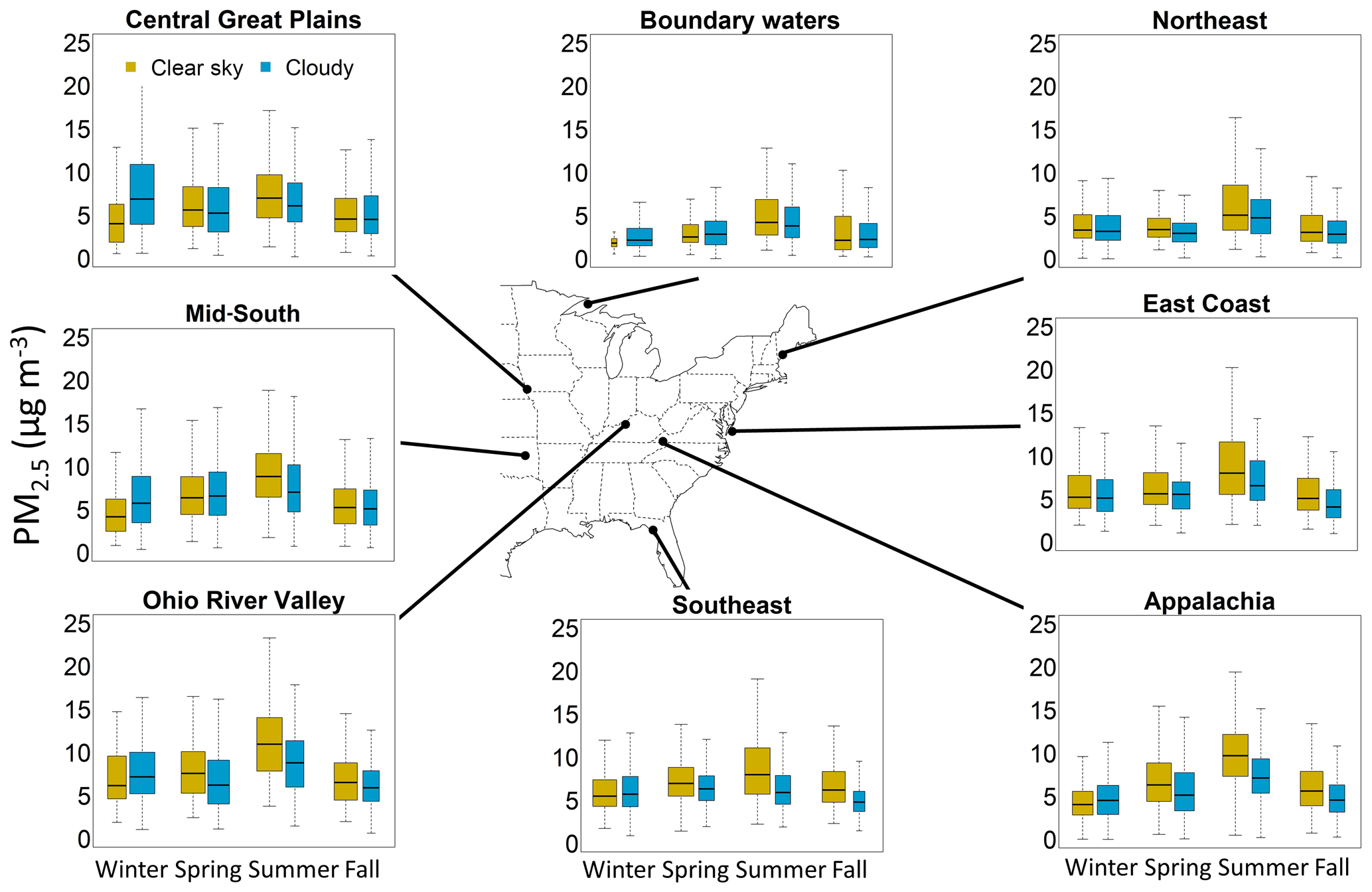
Figure 1Differences in PM2.5 mass concentrations in the eastern US. Clear-sky values are yellow and cloudy are blue. Median values are shown as a midline with box boundaries as the 75th and 25th percentiles. Whiskers are the 90th and 10th percentiles. Outliers are not shown but are included in calculations. PM2.5 mass is typically highest during clear-sky conditions with the exception of winter.
There is evidence that successful retrieval frequency contributes to a clear-sky bias in satellite AOT products when compared to surface PM2.5 measurements at IMPROVE monitoring locations in the eastern US. Across the CONUS, significant differences in PM2.5 mass concentrations measured at IMPROVE monitoring locations are observed between cloudy and clear-sky conditions in the majority (> 60 %) of regions in any given season during 2010–2014 (Fig. 1 and A1; Table S2 in the Supplement), especially during summer. Median all-sky PM2.5 concentrations are also significantly different and typically lower than clear-sky in multiple chemical climatology regions (Table S3 in the Supplement). Similarly, Christopher and Gupta (2010) found that cloudy and all-sky PM2.5 surface mass concentrations differed by 2.5 µg m−3 for the CONUS in 2006, but differences in that work were not statistically significant as they are here. This may be due to differing regional and temporal aggregation, the considered timeframes, and clear-sky definitions. In that work, a day was defined as clear-sky if one pixel in the 5 × 5 grid had a successful AOT retrieval, whereas we take the 44.4 % approach described above. In all regions, clear-sky PM2.5 concentrations are generally higher than cloudy with some exceptions during winter. There is an increased likelihood of aerosol removal due to scavenging by precipitation during cloudy times, and this may contribute to differences in mass concentrations. However, the cloud definition employed here uses the entire column (i.e., non-precipitating cirrus and stratus clouds are included), and the majority of cloud droplets evaporate (Pruppacher and Klett, 2010). Further, differences in PM2.5 mass concentrations are not a quantitative function of MODIS cloud fraction values during any season in any region (Fig. S7 in the Supplement), yet this work suggests that further study with a more sophisticated analysis of cloud properties is warranted.
3.2 PM2.5 chemical composition
Differences in daily mass concentrations during cloudy and clear-sky periods across the CONUS are spatially and temporally different among PM2.5 mass and its chemical constituents except in the Northwest region (Figs. 2 and A2–A5; Tables S2 and S4–S12 in the Supplement). Overall patterns for individual chemical constituents cannot be quantitatively described as a function of MODIS cloud fraction (Figs. S7 and S9 in the Supplement). If physical meteorology was the only controlling factor differentiating aerosol concentrations between clear-sky and cloudy times, then patterns among PM2.5 and constituents should be similar. However, they vary (Fig. 2). This suggests that changing emissions and/or in situ chemistry contribute to distinct patterns among PM2.5 chemical constituents.
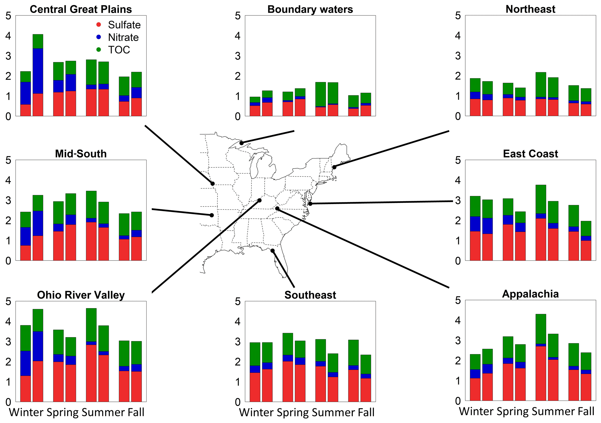
Figure 2Seasonal median values of PM2.5 chemical constituents in the eastern US during MODIS-defined clear-sky (left stacked bar in each pair) and cloudy (right stacked bar in each pair) conditions. Total organic carbon mass concentrations are nearly universally higher during clear-sky conditions in all regions, and this pattern is unique among PM2.5 chemical constituents.
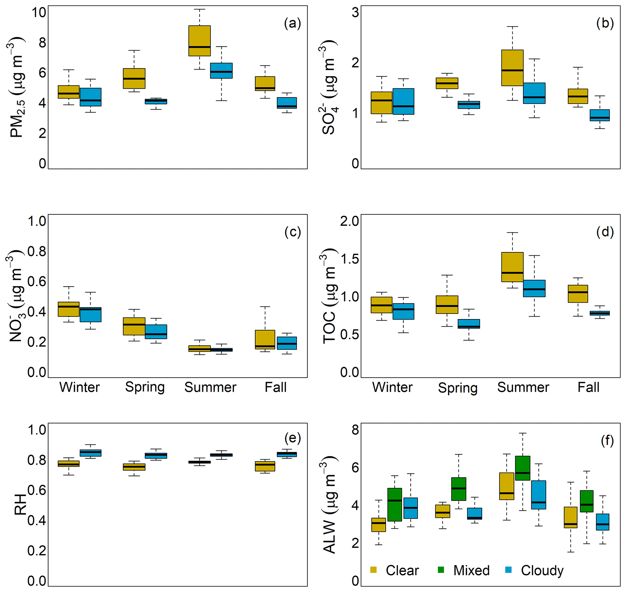
Figure 3Distributions of (a) PM2.5, (b) SO4, (c) NO3, (d) TOC, (e) RH, and (f) ALW mass concentrations during all seasons in the eastern US. Yellow box plots indicate clear-sky times, and blue box plots indicate cloudy times. In (b), the green box plots represent the mixed ALW scenario.
Clear-sky and cloudy patterns in and mass concentrations, which affect particle hygroscopicity, vary regionally and seasonally. Outside winter, sulfate mass concentrations are significantly higher on clear-sky days in the eastern US (Fig. 2, Table S4 in the Supplement), while nitrate concentrations are consistently highest under cloudy conditions. Higher clear-sky concentrations during summertime are associated with heat waves and stagnation events, which are characterized by a lack of ventilation in high-pressure systems (Jacob and Winner, 2009; Wang and Angell, 1999), and increased electricity demand (Farkas et al., 2016) associated with emissions that form sulfate. The sharpest clear-sky vs. cloudy differences in sulfate mass occur in the East Coast, Appalachia, Southeast, and Ohio River Valley. The highest nitrate concentrations occur during cloudy days in winter (Fig. 2, Table S5 in the Supplement), which are cooler (Table S8 in the Supplement) and promote the thermodynamic stability of nitrate in the condensed phase. The sharpest differences in nitrate occur in the Central Great Plains.

Figure 4Distributions of (a) inorganic ALW, (b) organic ALW, and (c) total (inorganic + organic) ALW during clear-sky (yellow) and cloudy (blue) times in all seasons across the CONUS. The width of the box plot is proportional to the number of observations that make up each distribution. Note that potential outliers are not shown but are used in calculations.
Mass concentrations of TOC are nearly always higher during clear-sky times than cloudy (Fig. 3, Table S6 in the Supplement) in all chemical climatology regions across the CONUS, with the largest differences during summer and fall. The patterns are unique among the PM2.5 chemical constituents and consistent with SOA. Summertime wildland fires in the west and prescribed burning during spring and fall in the east may obscure interpretation due to large episodic primary OC emissions (Spracklen et al., 2007; Tian et al., 2009; Zeng et al., 2008). However, at IMPROVE monitoring locations, the secondary organic aerosol (SOA) contribution to TOC dominates over primary sources (Carlton et al., 2018a). The most pronounced differences in clear-sky and cloudy TOC occur in summer in regions where precursor biogenic VOC emissions that form SOA are substantial (Donahue et al., 2009; Gentner et al., 2017; Youn et al., 2013). Further, increased sunlight and higher temperatures under clear-sky conditions (Table S8) lead to higher biogenic VOC emissions that form SOA (Laothawornkitkul et al., 2009; Sakulyanontvittaya et al., 2008) and enhanced photolysis rates that facilitate hydroxyl radical production important to SOA formation (Tang et al., 2003). These findings indicate that TOC mass concentrations are different on clear-sky and cloudy days and suggest organic composition changes as well.
Cloudy-period ALW mass concentrations are higher than clear-sky in all seasons from both inorganic and organic contributions, with few exceptions (Fig. 4, Table S7 in the Supplement). The largest cloudy and clear-sky ALW differences are observed in the central and eastern US during winter. The pattern of higher ALW during cloudy periods is opposite to the pattern of dry PM2.5 mass and arises from a combination of higher RH and changing aerosol composition that affects hygroscopicity. Nitrate is the most hygroscopic species considered in this analysis, and high cloudy mass concentrations increase particle hygroscopicity to facilitate ALW during these times, despite lower overall dry PM2.5 mass. Clear-sky and cloudy changes in the precise chemical composition of organic compounds and their impacts on ALW remain critical open questions.
3.3 ALW and growth factor scenarios in the eastern US
Distributions in monthly particle chemical composition across the eastern US in 2010–2014 are sufficiently changed between MODIS-defined cloudy and clear-sky times to affect hygroscopicity and alter predicted ALW mass concentrations beyond differences that would arise from changes in meteorology alone (Fig. 5). The only difference between the mixed and cloudy ALW calculations is that the mixed scenario employs clear-sky chemical composition (rather than cloudy chemical composition) extrapolated to cloudy meteorology. This type of scenario can occur in model development or satellite validation applications when PM2.5–AOD relationships or growth factors remain unmeasured for cloudy periods (Brock et al., 2016; van Donkelaar et al., 2010; de Hoogh et al., 2016; Tian and Chen, 2010). When clear-sky chemical composition is extrapolated to cloudy-period meteorology (mixed), monthly median ALW concentrations in the eastern US, in all seasons except winter, are significantly different from our best estimate, which employs the actual chemical composition during cloudy periods (cloudy). These findings are consistent with analyses showing that chemical composition is an essential factor for improving cloud condensation nuclei predictions (Crosbie et al., 2015), determining ALW (Carlton and Turpin, 2013; Liao and Seinfeld, 2005), and calculating extinction (Pitchford et al., 2007).
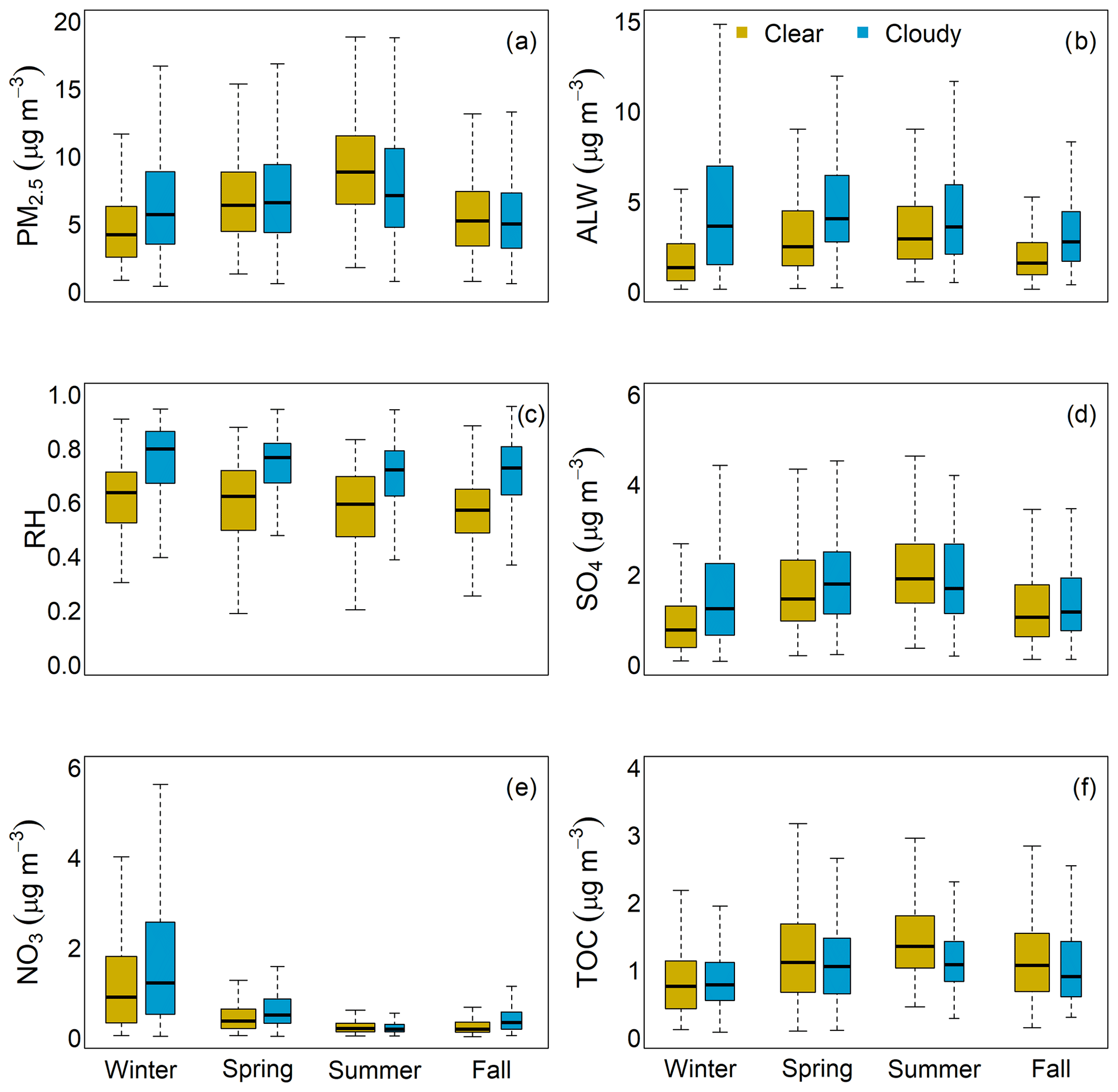
Figure 5Distributions of (a) PM2.5, (b) ALW, (c) RH, (d) SO4, (e) NO3, and (f) TOC mass concentrations in all seasons in the Mid-South. Yellow box plots indicate clear-sky times, and blue box plots indicate cloudy times. The width of the box plots is proportional to the number of observations in each. Note that potential outliers are not shown but are used in calculations.
Generally, mixed ALW concentrations in the eastern US are higher than for the cloudy scenario because clear-sky chemical composition facilitates greater hygroscopicity and cloudy RH is elevated (Table S7). A notable exception is the Ohio River Valley during winter, where cloudy , , and RH are higher than clear-sky. In this case, cloudy-period ALW concentrations are higher than for the mixed scenario. These findings highlight the fact that a changing PM2.5 chemical composition has a determining effect on ALW mass concentrations (Nguyen et al., 2016b), a critical element in the estimation of aerosol–cloud interactions and particle radiative impacts. Previous work using climate models shows that the application of ALW uptake that is influenced by incorrect chemical composition significantly affects top-of-atmosphere radiative forcing estimates and attribution of anthropogenic climate impacts (Rastak et al., 2017). During cloudy periods, when the accurate prediction of ALW and aerosol–cloud interactions is most critical, in situ knowledge of PM2.5 chemical composition is required.
3.4 Case study: the Mid-South
Table 1Particle chemical constituent concentrations, meteorology, and growth factors during cloudy (Cl) and clear-sky (CS) times in the Mid-South.
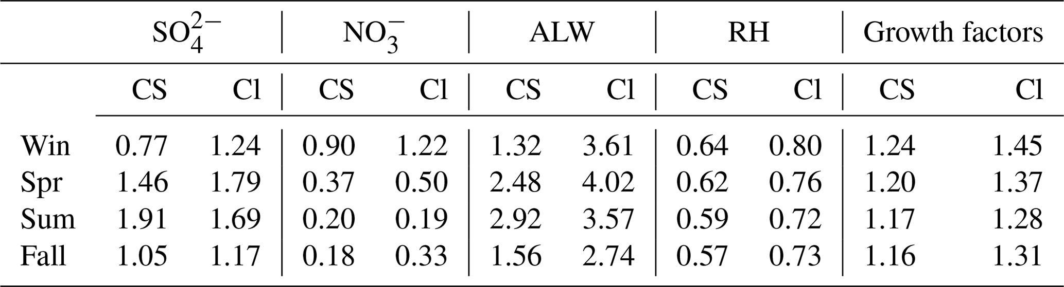
ALW concentrations are significantly higher during cloudy times than clear-sky in the Mid-South during all seasons (Table 1, Fig. 5). RH in the region is high year-round during cloudy and clear-sky periods alike, with the median greater than 60 %. This suggests that gas-phase water vapor mixing ratios are not limiting for ALW in the region for any season. Aerosol mass concentrations and chemical composition vary, however, and the effects on particle hygroscopicity can be seen in contrasting cloudy and clear-sky ALW concentrations among the seasons. During clear-sky conditions, the highest ALW mass concentrations occur during summer and spring, which correspond to the highest concentrations in the Mid-South, and not when clear-sky RH is highest (i.e., during winter). Year-round concentrations are higher during cloudy conditions than clear-sky. The largest absolute ALW concentrations and estimated growth factors occur during cloudy times in the winter and spring, when mass fraction and RH are highest. Nitrate concentrations are generally lower than , and while sulfate is thought to determine ALW mass concentrations in the region (Carlton and Turpin, 2013; Gasparini et al., 2006), is more hygroscopic. The Mid-South is a continental, agricultural area; in a separate but similar location, the Po Valley in Italy, was found to control ALW concentrations (Hodas et al., 2014). Independent humidified nephelometer measurements demonstrate that aerosol growth factors are highest in the winter and spring at the SGP site within the Mid-South chemical climatology region and identify nitrate and RH as determining factors (Jefferson et al., 2017). Observed growth factors by Jefferson et al. (2017) are higher than those estimated here, and we suspect this arises due to the presence of hygroscopic species such as ammonium, which is common to agricultural regions and not included in our ALW estimates.
Patterns in estimated growth factors suggest that the chemistry of water uptake by aerosol is different during cloudy and clear-sky periods and is related to changes in particle hygroscopicity driven by sulfate and nitrate pollution. Contributions from SOA, enhanced by anthropogenic emissions (Carlton et al., 2018a), also play a role, though it is difficult to accurately quantify. These patterns in changing aerosol hygroscopicity are consistent with findings for the central US demonstrating that cloud microphysics, mesoscale convective systems, and precipitation are impacted by anthropogenically influenced aerosol (Kawecki et al., 2016; Kawecki and Steiner, 2018).
Across the CONUS, statistically discernible differences among PM2.5 and chemical constituent concentrations under cloudy and clear-sky conditions cannot be explained solely by physical mechanisms. The chemical properties of aerosol are important to explain differences in water uptake and particle composition under different meteorological conditions. While meteorological phenomena such as pressure systems, winds, and air mixing affect PM2.5 and chemical component concentrations, they are insufficient to explain chemical constituent differences between cloudy and clear-sky times. In situ chemical information is necessary to fully explain temporal and spatial patterns. Spatially and seasonally, PM2.5 and particle speciation information that lends insight into water uptake, particle properties, and particle growth is incomplete when gathered only during clear-sky times. Differences in PM2.5 concentrations under different cloud conditions suggest a potential bias in the understanding of PM2.5 and AOT when using information only from clear-sky times. The work presented here indicates that aerosol growth due to water uptake is greatest during MODIS-defined periods identified as cloudy in many regions, when satellites are unable to remotely sense surface particle properties and impacts. This limits understanding of atmospheric particle burden and its climate-relevant physicochemical properties, which have implications for the prediction of weather (Kawecki and Steiner, 2018), air quality, and climate. This indicates that the clear-sky bias can affect accurate representation of ALW on cloudy days and suggests that without in situ chemical information, aerosol–cloud interactions, subsequent estimates of radiative forcings in models (Lin et al., 2016; Vogelmann et al., 2012), and feedbacks will remain a large uncertainty. This work suggests that further study employing new satellite algorithms and geostationary analysis is warranted.

Figure A1Maps of the difference in PM2.5 mass concentration medians (cloudy–clear-sky) for all regions from 2010 to 2014 for (a) winter, (b) spring, (c) summer, and (d) fall. The color of the point corresponds to the magnitude of the difference. Triangles indicate that median differences are significant according to the Mann–Whitney U test.
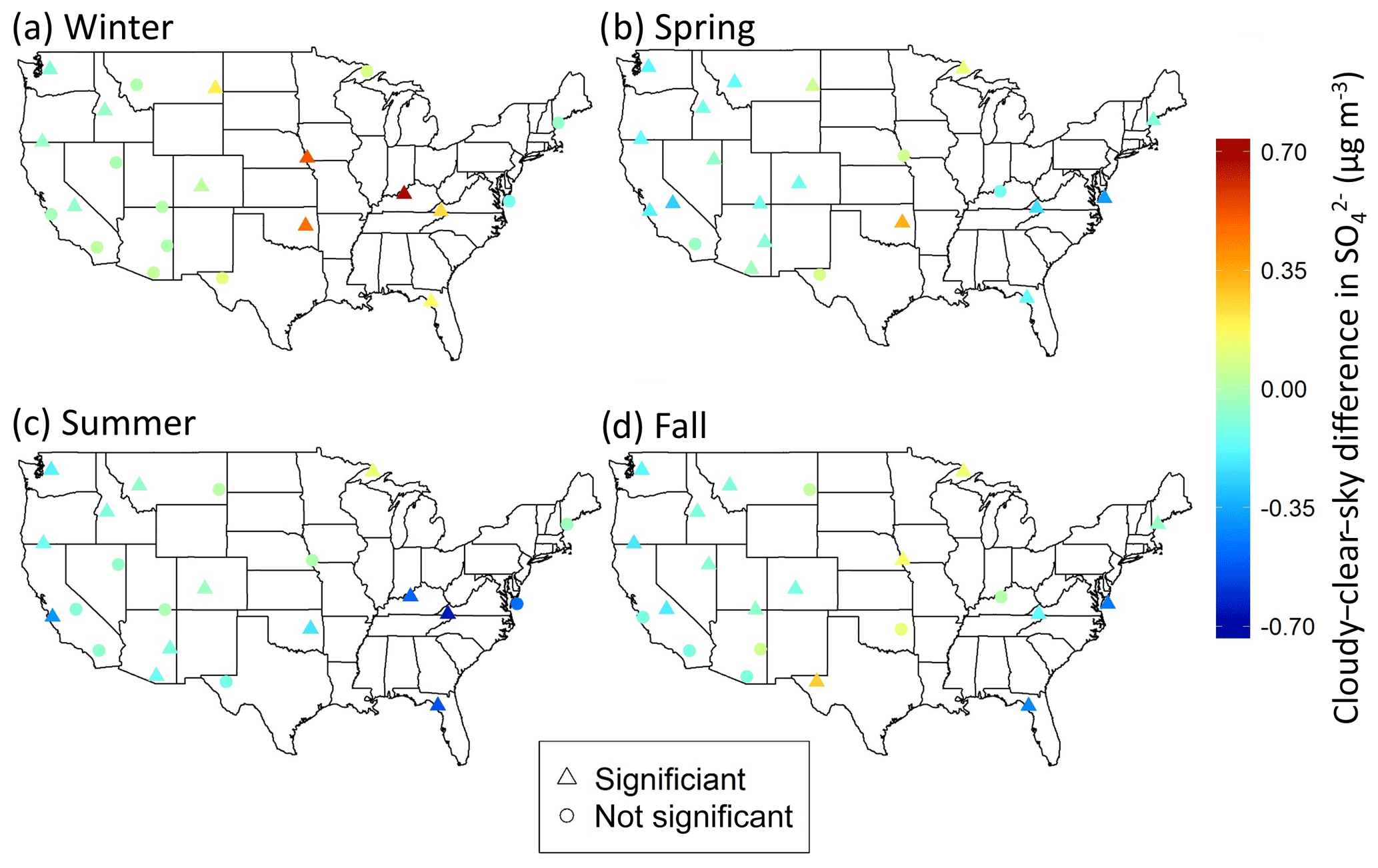
Figure A2Maps of the difference in mass concentration medians (cloudy–clear-sky) for all regions from 2010 to 2014 for (a) winter, (b) spring, (c) summer, and (d) fall. The color of the point corresponds to the magnitude of the difference. Triangles indicate that median differences are significant according to the Mann–Whitney U test.
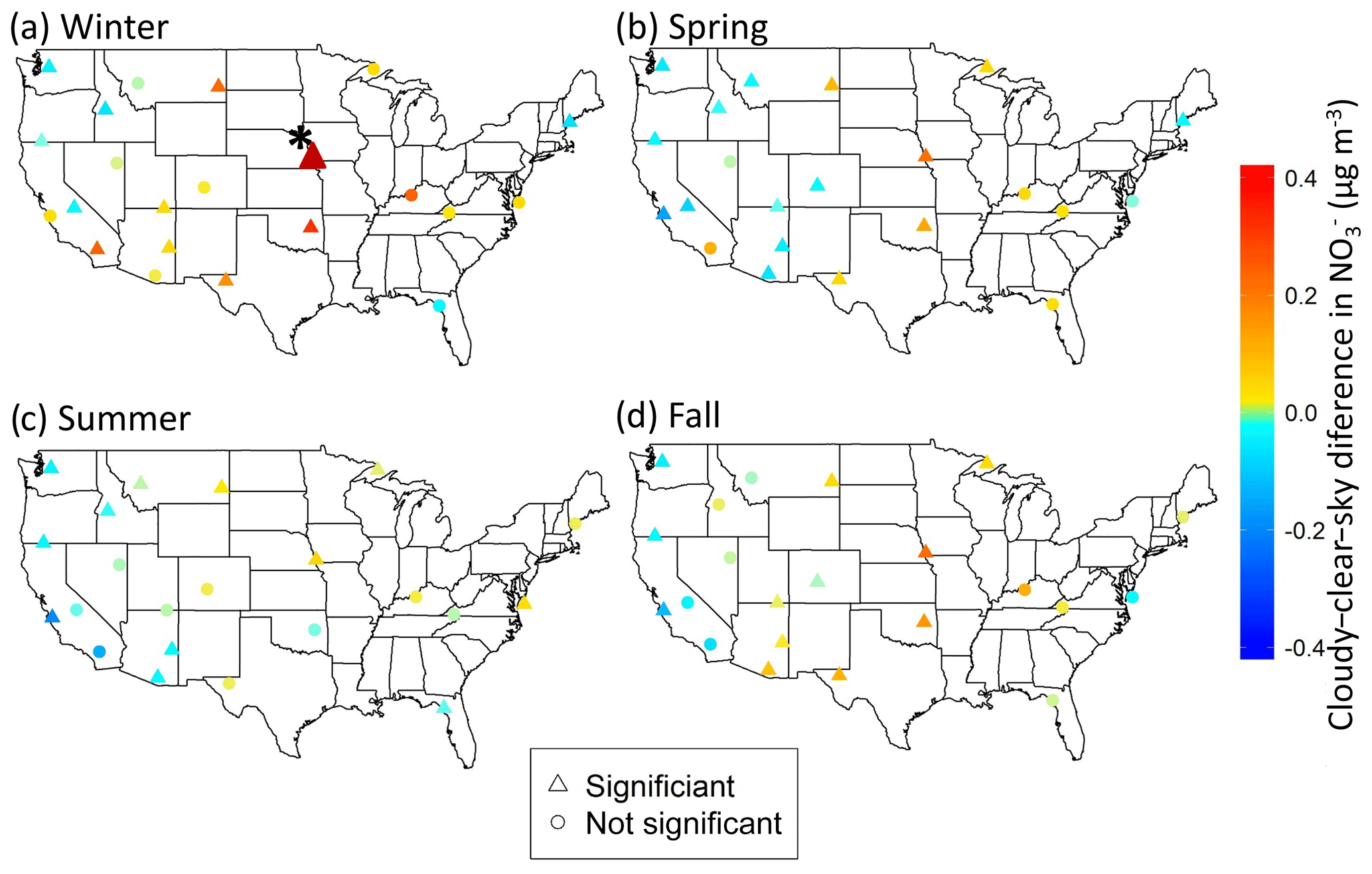
Figure A3Maps of the difference in mass concentration medians (cloudy–clear-sky) for all regions from 2010 to 2014 for (a) winter, (b) spring, (c) summer, and (d) fall. The color of the point corresponds to the magnitude of the difference. Triangles indicate that median differences are significant according to the Mann–Whitney U test. Note that the difference in medians for daily concentrations in winter for the Central Great Plains (denoted with asterisk) is substantially larger than other regions (the cloudy median value is 1.07 µg m−3 larger than clear-sky).
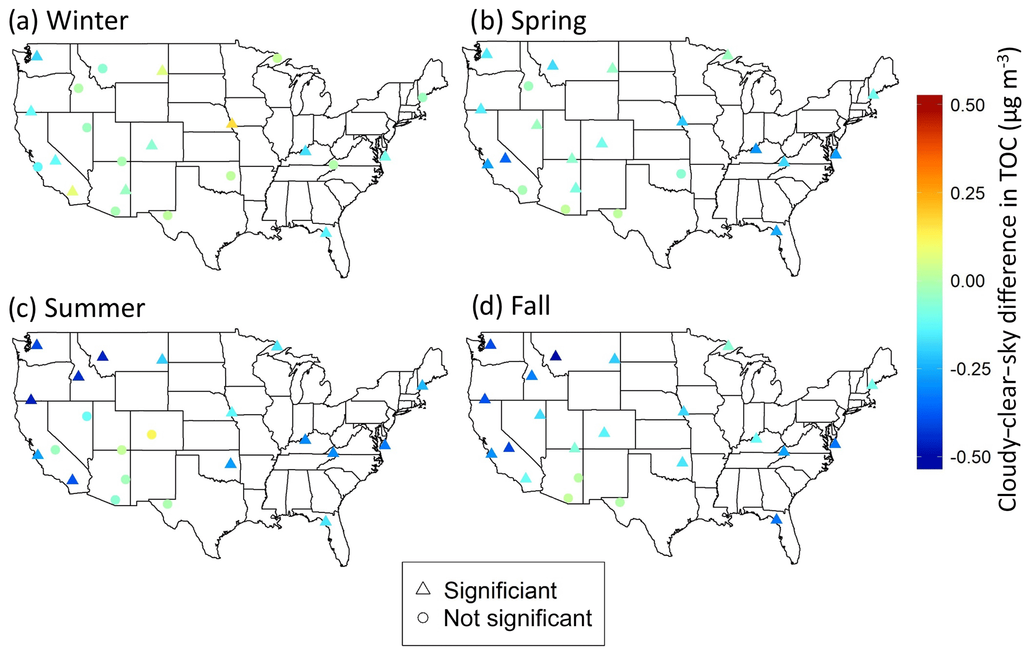
Figure A4Maps of the difference in TOC mass concentration medians (cloudy–clear-sky) for all regions from 2010 to 2014 for (a) winter, (b) spring, (c) summer, and (d) fall. The color of the point corresponds to the magnitude of the difference. Triangles indicate that median differences are significant according to the Mann–Whitney U test.
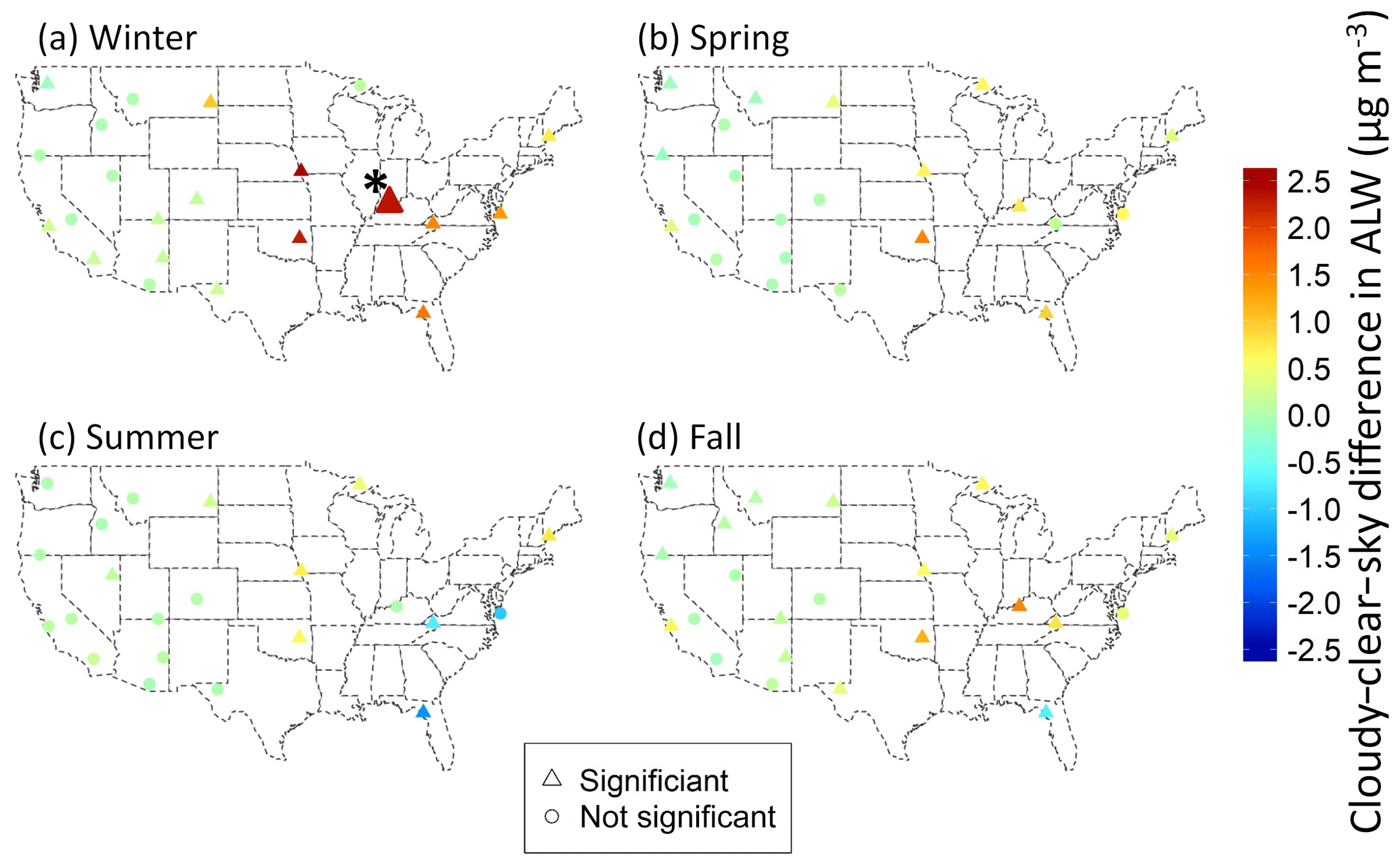
Figure A5Maps of the difference in ALW mass concentration medians (cloudy–clear-sky) for all regions from 2010 to 2014 for (a) winter, (b) spring, (c) summer, and (d) fall. The color of the point corresponds to the magnitude of the difference. Triangles indicate that median differences are significant according to the Mann–Whitney U test. Note that the difference in wintertime medians for daily ALW concentrations in the Ohio River Valley (denoted with an asterisk) is substantially larger than other regions (the cloudy median value is 4.6 µg m−3 larger than clear-sky).
The IMPROVE database can be found at https://views.cira.colostate.edu/fed/QueryWizard/ (last access: 4 April 2019). NCEP Reanalysis data are available from the NOAA/OAR/ESRL PSD in Boulder, Colorado, United States, at https://psl.noaa.gov/data/gridded/data.narr.html (NOAA/OAR/ESRL PSD, 2018, last access: 24 October 2018). MODIS data were acquired from the NASA Global Change Master Directory (GCMD) at https://search.earthdata.nasa.gov/portal/idn/search?q=modis&ac=true (NASA Global Change Master Directory (GCMD), last access: 5 October 2020).
The supplement related to this article is available online at: https://doi.org/10.5194/acp-20-11607-2020-supplement.
AGC designed the study. BHH paired satellite and surface data. AEC did all calculations with support from AGC and BHH. AEC wrote the paper with support and editing from AGC and BHH.
The authors declare that they have no conflict of interest.
The views expressed in this paper are those of the authors and do not necessarily reflect the views or policies of the U.S. Environmental Protection Agency.
This research was funded, in part, by NSF grant AGS-1242155, DOE grant DE-SC0018349, and NASA grant no. 80NSSC19K0987. The authors thank Virendra Ghate for support in retrieving NCEP Reanalysis data, as well as Divya Srivistava and Julia Daniels for technical support. The authors also thank Athanasios Nenes for the development and public availability of ISORROPIA.
This research has been supported by the National Science Foundation, Directorate for Geosciences (grant no. AGS-1242155), the National Aeronautics and Space Administration (grant no. 80NSSC19K0987), and the Atmospheric System Research (ASR), Program Department of Energy (DOE) (grant no. DE-SC0018349).
This paper was edited by Armin Sorooshian and reviewed by two anonymous referees.
Aswini, A. R., Hegde, P., Nair, P. R., and Aryasree, S.: Seasonal changes in carbonaceous aerosols over a tropical coastal location in response to meteorological processes, Sci. Total Environ., 656, 1261–1279, https://doi.org/10.1016/j.scitotenv.2018.11.366, 2019.
Babila, J. E., Carlton, A. G., Hennigan, C. J., and Ghate, V. P.: On Aerosol Liquid Water and Sulfate Associations: The Potential for Fine Particulate Matter Biases, Atmosphere, 11, 1–11, https://doi.org/10.3390/atmos11020194, 2020.
Bar-Or, R. Z., Koren, I., Altaratz, O., and Fredj, E.: Radiative properties of humidified aerosols in cloudy environment, Atmos. Res., 118, 280–294, https://doi.org/10.1016/j.atmosres.2012.07.014, 2012.
Bray, C. D., Battye, W., Aneja, V. P., Tong, D., Lee, P., Tang, Y., and Nowak, J. B.: Evaluating ammonia (NH3) predictions in the NOAA National Air Quality Forecast Capability (NAQFC) using in-situ aircraft and satellite measurements from the CalNex2010 campaign, Atmos. Environ., 163, 65–76, https://doi.org/10.1016/j.atmosenv.2017.05.032, 2017.
Brock, C. A., Wagner, N. L., Anderson, B. E., Attwood, A. R., Beyersdorf, A., Campuzano-Jost, P., Carlton, A. G., Day, D. A., Diskin, G. S., Gordon, T. D., Jimenez, J. L., Lack, D. A., Liao, J., Markovic, M. Z., Middlebrook, A. M., Ng, N. L., Perring, A. E., Richardson, M. S., Schwarz, J. P., Washenfelder, R. A., Welti, A., Xu, L., Ziemba, L. D., and Murphy, D. M.: Aerosol optical properties in the southeastern United States in summer – Part 1: Hygroscopic growth, Atmos. Chem. Phys., 16, 4987–5007, https://doi.org/10.5194/acp-16-4987-2016, 2016.
Cao, J. J., Wu, F., Chow, J. C., Lee, S. C., Li, Y., Chen, S. W., An, Z. S., Fung, K. K., Watson, J. G., Zhu, C. S., and Liu, S. X.: Characterization and source apportionment of atmospheric organic and elemental carbon during fall and winter of 2003 in Xi'an, China, Atmos. Chem. Phys., 5, 3127–3137, https://doi.org/10.5194/acp-5-3127-2005, 2005.
Carlton, A. G. and Turpin, B. J.: Particle partitioning potential of organic compounds is highest in the Eastern US and driven by anthropogenic water, Atmos. Chem. Phys., 13, 10203–10214, https://doi.org/10.5194/acp-13-10203-2013, 2013.
Carlton, A. G., Turpin, B. J., Altieri, K. E., Seitzinger, S. P., Mathur, R., Roselle, S. J., and Weber, R. J.: CMAQ Model Performance Enhanced When In-Cloud Secondary Organic Aerosol is Included: Comparisons of Organic Carbon Predictions with Measurements, Environ. Sci. Technol., 42, 8798–8802, https://doi.org/10.1021/es801192n, 2008.
Carlton, A. G., Pye, H. O. T., Baker, K. R., and Hennigan, C. J.: Additional Benefits of Federal Air-Quality Rules: Model Estimates of Controllable Biogenic Secondary Organic Aerosol, Environ. Sci. Technol., 52, 9254–9265, https://doi.org/10.1021/acs.est.8b01869, 2018a.
Carlton, A. G., de Gouw, J., Jimenez, J. L., Ambrose, J. L., Attwood, A. R., Brown, S., Baker, K. R., Brock, C., Cohen, R. C., Edgerton, S., Farkas, C. M., Farmer, D., Goldstein, A. H., Gratz, L., Guenther, A., Hunt, S., Jaeglé, L., Jaffe, D. A., Mak, J., McClure, C., Nenes, A., Nguyen, T. K., Pierce, J. R., de Sa, S., Selin, N. E., Shah, V., Shaw, S., Shepson, P. B., Song, S., Stutz, J., Surratt, J. D., Turpin, B. J., Warneke, C., Washenfelder, R. A., Wennberg, P. O., and Zhou, X.: Synthesis of the Southeast Atmosphere Studies: Investigating Fundamental Atmospheric Chemistry Questions, B. Am. Meteorol. Soc., 99, 547–567, https://doi.org/10.1175/BAMS-D-16-0048.1, 2018b.
Carlton, A. G, Christiansen, A. E., Flesch, M. M., Hennigan, C. J., and Sareen, N.: Multiphase Atmospheric Chemistry in Liquid Water: Impacts and Controllability of Organic Aerosol, Accounts Chem. Res., 53, 1715–1723, https://doi.org/10.1021/acs.accounts.0c00301, 2020.
Chang, R. Y.-W., Slowik, J. G., Shantz, N. C., Vlasenko, A., Liggio, J., Sjostedt, S. J., Leaitch, W. R., and Abbatt, J. P. D.: The hygroscopicity parameter (κ) of ambient organic aerosol at a field site subject to biogenic and anthropogenic influences: relationship to degree of aerosol oxidation, Atmos. Chem. Phys., 10, 5047–5064, https://doi.org/10.5194/acp-10-5047-2010, 2010.
Chow, J. C., Watson, J. G., Kuhns, H., Etyemezian, V., Lowenthal, D. H., Crow, D., Kohl, S. D., Engelbrecht, J. P., and Green, M. C.: Source profiles for industrial, mobile, and area sources in the Big Bend Regional Aerosol Visibility and Observational study, Chemosphere, 54, 185–208, https://doi.org/10.1016/j.chemosphere.2003.07.004, 2004.
Christiansen, A., Carlton, A. M. G., and Porter, W. C.: The changing nature of organic carbon over the United States, Environ. Sci. Technol., 54, 10524–10532, https://doi.org/10.1021/acs.est.0c02225, 2020.
Christiansen, A. E., Ghate, V. P., and Carlton, A. G.: Aerosol Optical Thickness: Organic Composition, Associated Particle Water, and Aloft Extinction, ACS Earth and Space Chemistry, 3, 403–412, https://doi.org/10.1021/acsearthspacechem.8b00163, 2019.
Christopher, S. A. and Gupta, P.: Satellite Remote Sensing of Particulate Matter Air Quality: The Cloud-Cover Problem, JAPCA J. Air Waste Ma., 60, 596–602, https://doi.org/10.3155/1047-3289.60.5.596, 2010.
Crosbie, E., Youn, J.-S., Balch, B., Wonaschütz, A., Shingler, T., Wang, Z., Conant, W. C., Betterton, E. A., and Sorooshian, A.: On the competition among aerosol number, size and composition in predicting CCN variability: a multi-annual field study in an urbanized desert, Atmos. Chem. Phys., 15, 6943–6958, https://doi.org/10.5194/acp-15-6943-2015, 2015.
de Hoogh, K., Gulliver, J., Donkelaar, A. van, Martin, R. V., Marshall, J. D., Bechle, M. J., Cesaroni, G., Pradas, M. C., Dedele, A., Eeftens, M., Forsberg, B., Galassi, C., Heinrich, J., Hoffmann, B., Jacquemin, B., Katsouyanni, K., Korek, M., Künzli, N., Lindley, S. J., Lepeule, J., Meleux, F., de Nazelle, A., Nieuwenhuijsen, M., Nystad, W., Raaschou-Nielsen, O., Peters, A., Peuch, V.-H., Rouil, L., Udvardy, O., Slama, R., Stempfelet, M., Stephanou, E. G., Tsai, M. Y., Yli-Tuomi, T., Weinmayr, G., Brunekreef, B., Vienneau, D., and Hoek, G.: Development of West-European PM2.5 and NO2 land use regression models incorporating satellite-derived and chemical transport modelling data, Environ. Res., 151, 1–10, https://doi.org/10.1016/j.envres.2016.07.005, 2016.
Donahue, N. M., Robinson, A. L., and Pandis, S. N.: Atmospheric organic particulate matter: From smoke to secondary organic aerosol, Atmos. Environ., 43, 94–106, https://doi.org/10.1016/j.atmosenv.2008.09.055, 2009.
Duong, H. T., Sorooshian, A., Craven, J. S., Hersey, S. P., Metcalf, A. R., Zhang, X., Weber, R. J., Jonsson, H., Flagan, R. C., and Seinfeld, J. H.: Water-soluble organic aerosol in the Los Angeles Basin and outflow regions: Airborne and ground measurements during the 2010 CalNex field campaign, J. Geophys. Res.-Atmos., 116, D00V04, https://doi.org/10.1029/2011JD016674, 2011.
Ervens, B., Sorooshian, A., Aldhaif, A. M., Shingler, T., Crosbie, E., Ziemba, L., Campuzano-Jost, P., Jimenez, J. L., and Wisthaler, A.: Is there an aerosol signature of chemical cloud processing?, Atmos. Chem. Phys., 18, 16099–16119, https://doi.org/10.5194/acp-18-16099-2018, 2018.
Fan, J., Wang, Y., Rosenfeld, D., and Liu, X.: Review of Aerosol–Cloud Interactions: Mechanisms, Significance, and Challenges, J. Atmos. Sci., 73, 4221–4252, https://doi.org/10.1175/JAS-D-16-0037.1, 2016.
Farkas, C. M., Moeller, M. D., Felder, F. A., Henderson, B. H., and Carlton, A. G.: High Electricity Demand in the Northeast U.S.: PJM Reliability Network and Peaking Unit Impacts on Air Quality, Environ. Sci. Technol., 50, 8375–8384, https://doi.org/10.1021/acs.est.6b01697, 2016.
Fountoukis, C. and Nenes, A.: ISORROPIA II: a computationally efficient thermodynamic equilibrium model for K+–Ca2+–Mg2+–NH4+–Na+–––Cl−–H2O aerosols, Atmos. Chem. Phys., 7, 4639–4659, https://doi.org/10.5194/acp-7-4639-2007, 2007.
Gasparini, R., Li, R., Collins, D. R., Ferrare, R. A., and Brackett, V. G.: Application of aerosol hygroscopicity measured at the Atmospheric Radiation Measurement Program's Southern Great Plains site to examine composition and evolution, J. Geophys. Res., 111, D05S12, https://doi.org/10.1029/2004JD005448, 2006.
Gentner, D. R., Jathar, S. H., Gordon, T. D., Bahreini, R., Day, D. A., El Haddad, I., Hayes, P. L., Pieber, S. M., Platt, S. M., de Gouw, J., Goldstein, A. H., Harley, R. A., Jimenez, J. L., Prévôt, A. S. H., and Robinson, A. L.: Review of Urban Secondary Organic Aerosol Formation from Gasoline and Diesel Motor Vehicle Emissions, Environ. Sci. Technol., 51, 1074–1093, https://doi.org/10.1021/acs.est.6b04509, 2017.
Guo, H., Xu, L., Bougiatioti, A., Cerully, K. M., Capps, S. L., Hite Jr., J. R., Carlton, A. G., Lee, S.-H., Bergin, M. H., Ng, N. L., Nenes, A., and Weber, R. J.: Fine-particle water and pH in the southeastern United States, Atmos. Chem. Phys., 15, 5211–5228, https://doi.org/10.5194/acp-15-5211-2015, 2015.
Guo, Y., Tang, Q., Gong, D.-Y., and Zhang, Z.: Estimating ground-level PM2.5 concentrations in Beijing using a satellite-based geographically and temporally weighted regression model, Remote Sens. Environ., 198, 140–149, https://doi.org/10.1016/j.rse.2017.06.001, 2017.
Gupta, P., Christopher, S. A., Wang, J., Gehrig, R., Lee, Y., and Kumar, N.: Satellite remote sensing of particulate matter and air quality assessment over global cities, Atmos. Environ., 40, 5880–5892, https://doi.org/10.1016/j.atmosenv.2006.03.016, 2006.
Hand, J. L., Copeland, S. A., Day, D. E., Dillner, A. M., Indresand, H., Malm, W. C., McDad, C. E., Moore, Jr., C. T., Pitchford, M. L., Schichtel, B. A., and Watson, J. G.: Spatial and Seasonal Patterns and Temporal Variability of Haze and its Constituents in the United States: Report V, available at: http://vista.cira.colostate.edu/improve/wp-content/uploads/2016/08/IMPROVE_V_FullReport.pdf (last access: 18 March 2018), 2011.
Hauser, A.: NOAA AVHRR derived aerosol optical depth over land, J. Geophys. Res., 110, D08204, https://doi.org/10.1029/2004JD005439, 2005.
Hinks, M. L., Montoya-Aguilera, J., Ellison, L., Lin, P., Laskin, A., Laskin, J., Shiraiwa, M., Dabdub, D., and Nizkorodov, S. A.: Effect of relative humidity on the composition of secondary organic aerosol from the oxidation of toluene, Atmos. Chem. Phys., 18, 1643–1652, https://doi.org/10.5194/acp-18-1643-2018,
Hodas, N., Sullivan, A. P., Skog, K., Keutsch, F. N., Collett, J. L., Decesari, S., Facchini, M. C., Carlton, A. G., Laaksonen, A., and Turpin, B. J.: Aerosol Liquid Water Driven by Anthropogenic Nitrate: Implications for Lifetimes of Water-Soluble Organic Gases and Potential for Secondary Organic Aerosol Formation, Environ. Sci. Technol., 48, 11127–11136, https://doi.org/10.1021/es5025096, 2014.
Hsu, N. C., Tsay, S.-C., King, M. D., and Herman, J. R.: Aerosol Properties Over Bright-Reflecting Source Regions, IEEE T. Geosci. Remote, 42, 557–569, https://doi.org/10.1109/TGRS.2004.824067, 2004.
Hsu, N. C., Tsay, S.-C., King, M. D., and Herman, J. R.: Deep Blue Retrievals of Asian Aerosol Properties During ACE-Asia, IEEE T. Geosci. Remote, 44, 3180–3195, https://doi.org/10.1109/TGRS.2006.879540, 2006.
Hsu, N. C., Jeong, M.-J., Bettenhausen, C., Sayer, A. M., Hansell, R., Seftor, C. S., Huang, J., and Tsay, S.-C.: Enhanced Deep Blue aerosol retrieval algorithm: The second generation, J. Geophys. Res.-Atmos., 118, 9296–9315, https://doi.org/10.1002/jgrd.50712, 2013.
IMPROVE Network: Federal Land Manager Environmental Database, available at: http://views.cira.colostate.edu/fed/DataWizard/Default.aspx (last access: 26 May 2016), 2019.
Jacob, D. J. and Winner, D. A.: Effect of climate change on air quality, Atmos. Environ., 43, 51–63, https://doi.org/10.1016/j.atmosenv.2008.09.051, 2009.
Jathar, S. H., Mahmud, A., Barsanti, K. C., Asher, W. E., Pankow, J. F., and Kleeman, M. J.: Water uptake by organic aerosol and its influence on gas/particle partitioning of secondary organic aerosol in the United States, Atmos. Environ., 129, 142–154, https://doi.org/10.1016/j.atmosenv.2016.01.001, 2016.
Jefferson, A., Hageman, D., Morrow, H., Mei, F., and Watson, T.: Seven years of aerosol scattering hygroscopic growth measurements from SGP: Factors influencing water uptake: Aerosol Scattering Hygroscopic Growth, J. Geophys. Res.-Atmos., 122, 9451–9466, https://doi.org/10.1002/2017JD026804, 2017.
Jones, T. A. and Christopher, S. A.: Satellite and Radar Remote Sensing of Southern Plains Grass Fires: A Case Study, J. Appl. Meteorol. Clim., 49, 2133–2146, https://doi.org/10.1175/2010JAMC2472.1, 2010.
Ju, J. and Roy, D. P.: The availability of cloud-free Landsat ETM+ data over the conterminous United States and globally, Remote Sens. Environ., 112, 1196–1211, https://doi.org/10.1016/j.rse.2007.08.011, 2008.
Kahn, R. A.: Multiangle Imaging Spectroradiometer (MISR) global aerosol optical depth validation based on 2 years of coincident Aerosol Robotic Network (AERONET) observations, J. Geophys. Res., 110, D10S04, https://doi.org/10.1029/2004JD004706, 2005.
Kalnay, E., Kanamitsu, M., Kistler, R., Collins, W., Deaven, D., Gandin, L., Iredell, M., Saha, S., White, G., Woollen, J., Zhu, Y., Leetmaa, A., Reynolds, R., Chelliah, M., Ebisuzaki, W., Higgins, W., Janowiak, J., Mo, K. C., Ropelewski, C., Wang, J., Jenne, R., and Joseph, D.: The NCEP/NCAR 40-Year Reanalysis Project, B. Am. Meteorol. Soc., 77, 437–471, https://doi.org/10.1175/1520-0477(1996)077<0437:TNYRP>2.0.CO;2, 1996.
Kamens, R. M., Zhang, H., Chen, E. H., Zhou, Y., Parikh, H. M., Wilson, R. L., Galloway, K. E., and Rosen, E. P.: Secondary organic aerosol formation from toluene in an atmospheric hydrocarbon mixture: Water and particle seed effects, Atmos. Environ., 45, 2324–2334, https://doi.org/10.1016/j.atmosenv.2010.11.007, 2011.
Kawecki, S. and Steiner, A. L.: The Influence of Aerosol Hygroscopicity on Precipitation Intensity During a Mesoscale Convective Event, J. Geophys. Res.-Atmos., 123, 424–442, https://doi.org/10.1002/2017JD026535, 2018.
Kawecki, S., Henebry, G. M., and Steiner, A. L.: Effects of Urban Plume Aerosols on a Mesoscale Convective System, J. Atmos. Sci., 73, 4641–4660, https://doi.org/10.1175/JAS-D-16-0084.1, 2016.
Kessner, A. L., Wang, J., Levy, R. C., and Colarco, P. R.: Remote sensing of surface visibility from space: A look at the United States East Coast, Atmos. Environ., 81, 136–147, https://doi.org/10.1016/j.atmosenv.2013.08.050, 2013.
King, M. D., Platnick, S., Menzel, W. P., Ackerman, S. A., and Hubanks, P. A.: Spatial and Temporal Distribution of Clouds Observed by MODIS Onboard the Terra and Aqua Satellites, IEEE T. Geosci. Remote, 51, 3826–3852, https://doi.org/10.1109/TGRS.2012.2227333, 2013.
Kloog, I., Koutrakis, P., Coull, B. A., Lee, H. J., and Schwartz, J.: Assessing temporally and spatially resolved PM2.5 exposures for epidemiological studies using satellite aerosol optical depth measurements, Atmos. Environ., 45, 6267–6275, https://doi.org/10.1016/j.atmosenv.2011.08.066, 2011.
Kovalskyy, V. and Roy, D.: A One Year Landsat 8 Conterminous United States Study of Cirrus and Non-Cirrus Clouds, Remote Sens.-Basel, 7, 564–578, https://doi.org/10.3390/rs70100564, 2015.
Kumar, N., Chu, A., and Foster, A.: An empirical relationship between PM2.5 and aerosol optical depth in Delhi Metropolitan, Atmos. Environ., 41, 4492–4503, https://doi.org/10.1016/j.atmosenv.2007.01.046, 2007.
Lamkaddam, H., Gratien, A., Pangui, E., Cazaunau, M., Picquet-Varrault, B., and Doussin, J.-F.: High-NOx Photooxidation of n-Dodecane: Temperature Dependence of SOA Formation, Environ. Sci. Technol., 51, 192–201, https://doi.org/10.1021/acs.est.6b03821, 2017.
Laothawornkitkul, J., Taylor, J. E., Paul, N. D., and Hewitt, C. N.: Biogenic volatile organic compounds in the Earth system, New Phytol., 183, 27–51, https://doi.org/10.1111/j.1469-8137.2009.02859.x, 2009.
Li, L., Gong, J., and Zhou, J.: Spatial Interpolation of Fine Particulate Matter Concentrations Using the Shortest Wind-Field Path Distance, edited by: Sun, Q., PLoS ONE, 9, e96111, https://doi.org/10.1371/journal.pone.0096111, 2014.
Liao, H. and Seinfeld, J. H.: Global impacts of gas-phase chemistry-aerosol interactions on direct radiative forcing by anthropogenic aerosols and ozone, J. Geophys. Res., 110, D18208, https://doi.org/10.1029/2005JD005907, 2005.
Lin, Y., Wang, Y., Pan, B., Hu, J., Liu, Y., and Zhang, R.: Distinct Impacts of Aerosols on an Evolving Continental Cloud Complex during the RACORO Field Campaign, J. Atmos. Sci., 73, 3681–3700, https://doi.org/10.1175/JAS-D-15-0361.1, 2016.
Liu, B., Ma, Y., Gong, W., Zhang, M., Wang, W., and Shi, Y.: Comparison of AOD from CALIPSO, MODIS, and Sun Photometer under Different Conditions over Central China, Sci. Rep.-UK, 8, 10066, https://doi.org/10.1038/s41598-018-28417-7, 2018.
Liu, Y., Schichtel, B. A., and Koutrakis, P.: Estimating Particle Sulfate Concentrations Using MISR Retrieved Aerosol Properties, IEEE J. Sel. Top. Appl., 2, 176–184, https://doi.org/10.1109/JSTARS.2009.2030153, 2009.
Liu, Y., Wang, Z., Wang, J., Ferrare, R. A., Newsom, R. K., and Welton, E. J.: The effect of aerosol vertical profiles on satellite-estimated surface particle sulfate concentrations, Remote Sens. Environ., 115, 508–513, https://doi.org/10.1016/j.rse.2010.09.019, 2011.
Malm, W. C., Sisler, J. F., Huffman, D., Eldred, R. A., and Cahill, T. A.: Spatial and seasonal trends in particle concentration and optical extinction in the United States, J. Geophys. Res., 99, 1347, https://doi.org/10.1029/93JD02916, 1994.
Malm, W. C., Schichtel, B. A., Hand, J. L., and Collett, J. L.: Concurrent Temporal and Spatial Trends in Sulfate and Organic Mass Concentrations Measured in the IMPROVE Monitoring Program: Trends in Sulfate and Organic Mass, J. Geophys. Res.-Atmos., 122, 10462–10476, https://doi.org/10.1002/2017JD026865, 2017.
Martin, R. V.: Satellite remote sensing of surface air quality, Atmos. Environ., 42, 7823–7843, https://doi.org/10.1016/j.atmosenv.2008.07.018, 2008.
McKeen, S., Grell, G., Peckham, S., Wilczak, J., Djalalova, I., Hsie, E.-Y., Frost, G., Peischl, J., Schwarz, J., Spackman, R., Holloway, J., de Gouw, J., Warneke, C., Gong, W., Bouchet, V., Gaudreault, S., Racine, J., McHenry, J., McQueen, J., Lee, P., Tang, Y., Carmichael, G. R., and Mathur, R.: An evaluation of real-time air quality forecasts and their urban emissions over eastern Texas during the summer of 2006 Second Texas Air Quality Study field study, J. Geophys. Res., 114, D00F11, https://doi.org/10.1029/2008JD011697, 2009.
McKnight, P. E. and Najab, J.: Mann–Whitney U Test, in: The Corsini Encyclopedia of Psychology, edited by: Weiner, I. B. and Craighead, W. E., John Wiley & Sons, Inc., Hoboken, NJ, USA, 2010.
Meng, Z. and Seinfeld, J. H.: On the Source of the Submicrometer Droplet Mode of Urban and Regional Aerosols, Aerosol Sci. Techn., 20, 253–265, https://doi.org/10.1080/02786829408959681, 1994.
Metzger, S., Abdelkader, M., Steil, B., and Klingmüller, K.: Aerosol water parameterization: long-term evaluation and importance for climate studies, Atmos. Chem. Phys., 18, 16747–16774, https://doi.org/10.5194/acp-18-16747-2018, 2018.
NASA Global Change Master Directory (GCMD): https://idn.ceos.org/, last access: 5 October 2020.
National Aeronautics and Space Administration: Global Change Master Directory, available at: https://gcmd.nasa.gov/ (last access: 20 May 2020), 2018.
Ng, N. L., Kroll, J. H., Chan, A. W. H., Chhabra, P. S., Flagan, R. C., and Seinfeld, J. H.: Secondary organic aerosol formation from m-xylene, toluene, and benzene, Atmos. Chem. Phys., 7, 3909–3922, https://doi.org/10.5194/acp-7-3909-2007, 2007.
Nguyen, T. K. V., Petters, M. D., Suda, S. R., Guo, H., Weber, R. J., and Carlton, A. G.: Trends in particle-phase liquid water during the Southern Oxidant and Aerosol Study, Atmos. Chem. Phys., 14, 10911–10930, https://doi.org/10.5194/acp-14-10911-2014, 2014.
Nguyen, T. K. V., Capps, S. L., and Carlton, A. G.: Decreasing Aerosol Water Is Consistent with OC Trends in the Southeast U.S., Environ. Sci. Technol., 49, 7843–7850, https://doi.org/10.1021/acs.est.5b00828, 2015.
Nguyen, T. K. V., Ghate, V. P., and Carlton, A. G.: Reconciling satellite aerosol optical thickness and surface fine particle mass through aerosol liquid water, Geophys. Res. Lett., 43, 11903–11912, https://doi.org/10.1002/2016GL070994, 2016a.
Nguyen, T. K. V., Zhang, Q., Jimenez, J. L., Pike, M., Carlton, A. G.: Liquid Water: Ubiquitous Contributor to Aerosol Mass, Environ. Sci. Technol., 3, 257–263, 2016b.
NOAA/OAR/ESRL PSL: https://psl.noaa.gov/, Boulder, Colorado, USA, last access: 24 October 2018.
Norris, J. R., Allen, R. J., Evan, A. T., Zelinka, M. D., O'Dell, C. W., and Klein, S. A.: Evidence for climate change in the satellite cloud record, Nature, 536, 72–75, https://doi.org/10.1038/nature18273, 2016.
Petters, M. D. and Kreidenweis, S. M.: A single parameter representation of hygroscopic growth and cloud condensation nucleus activity, Atmos. Chem. Phys., 7, 1961–1971, https://doi.org/10.5194/acp-7-1961-2007, 2007.
Pitchford, M., Malm, W., Schichtel, B., Kumar, N., Lowenthal, D., and Hand, J.: Revised Algorithm for Estimating Light Extinction from IMPROVE Particle Speciation Data, JAPCA J. Air Waste Ma., 57, 1326–1336, https://doi.org/10.3155/1047-3289.57.11.1326, 2007.
Pratt, K. A., Fiddler, M. N., Shepson, P. B., Carlton, A. G., and Surratt, J. D.: Organosulfates in cloud water above the Ozarks' isoprene source region, Atmos. Environ., 77, 231–238, https://doi.org/10.1016/j.atmosenv.2013.05.011, 2013.
Pruppacher, H. R. and Klett, J. D.: Microphysics of clouds and precipitation, Springer, Dordrecht, New York, 2010.
R Core Team: R: A language and environment for statistical computing, R Foundation for Statistical Computing, Vienna, Austria, available at: http://www.R-project.org/ (last access: July 2020), 2013.
Rastak, N., Pajunoja, A., Acosta Navarro, J. C., Ma, J., Song, M., Partridge, D. G., Kirkevåg, A., Leong, Y., Hu, W. W., Taylor, N. F., Lambe, A., Cerully, K., Bougiatioti, A., Liu, P., Krejci, R., Petäjä, T., Percival, C., Davidovits, P., Worsnop, D. R., Ekman, A. M. L., Nenes, A., Martin, S., Jimenez, J. L., Collins, D. R., Topping, D. O., Bertram, A. K., Zuend, A., Virtanen, A., and Riipinen, I.: Microphysical explanation of the RH-dependent water affinity of biogenic organic aerosol and its importance for climate, Geophys. Res. Lett., 44, 5167–5177, https://doi.org/10.1002/2017GL073056, 2017.
Remer, L. A., Mattoo, S., Levy, R. C., and Munchak, L. A.: MODIS 3 km aerosol product: algorithm and global perspective, Atmos. Meas. Tech., 6, 1829–1844, https://doi.org/10.5194/amt-6-1829-2013, 2013.
Ryerson, T. B., Andrews, A. E., Angevine, W. M., Bates, T. S., Brock, C. A., Cairns, B., Cohen, R. C., Cooper, O. R., de Gouw, J. A., Fehsenfeld, F. C., Ferrare, R. A., Fischer, M. L., Flagan, R. C., Goldstein, A. H., Hair, J. W., Hardesty, R. M., Hostetler, C. A., Jimenez, J. L., Langford, A. O., McCauley, E., McKeen, S. A., Molina, L. T., Nenes, A., Oltmans, S. J., Parrish, D. D., Pederson, J. R., Pierce, R. B., Prather, K., Quinn, P. K., Seinfeld, J. H., Senff, C. J., Sorooshian, A., Stutz, J., Surratt, J. D., Trainer, M., Volkamer, R., Williams, E. J., and Wofsy, S. C.: The 2010 California Research at the Nexus of Air Quality and Climate Change (CalNex) field study, J. Geophys. Res.-Atmos., 118, 5830–5866, https://doi.org/10.1002/jgrd.50331, 2013.
Sakulyanontvittaya, T., Duhl, T., Wiedinmyer, C., Helmig, D., Matsunaga, S., Potosnak, M., Milford, J., and Guenther, A.: Monoterpene and Sesquiterpene Emission Estimates for the United States, Environ. Sci. Technol., 42, 1623–1629, https://doi.org/10.1021/es702274e, 2008.
Schaap, M., Apituley, A., Timmermans, R. M. A., Koelemeijer, R. B. A., and de Leeuw, G.: Exploring the relation between aerosol optical depth and PM2.5 at Cabauw, the Netherlands, Atmos. Chem. Phys., 9, 909–925, https://doi.org/10.5194/acp-9-909-2009, 2009.
Sisterson, D. L., Peppler, R. A., Cress, T. S., Lamb, P. J., and Turner, D. D.: The ARM Southern Great Plains (SGP) Site, Meteor. Mon., 57, 6.1–6.14, https://doi.org/10.1175/AMSMONOGRAPHS-D-16-0004.1, 2016.
Song, W., Jia, H., Huang, J., and Zhang, Y.: A satellite-based geographically weighted regression model for regional PM2.5 estimation over the Pearl River Delta region in China, Remote Sens. Environ., 154, 1–7, https://doi.org/10.1016/j.rse.2014.08.008, 2014.
Sorek-Hamer, M., Just, A. C., and Kloog, I.: Satellite remote sensing in epidemiological studies, Curr. Opin. Pediatr., 28, 228–234, https://doi.org/10.1097/MOP.0000000000000326, 2016.
Spracklen, D. V., Logan, J. A., Mickley, L. J., Park, R. J., Yevich, R., Westerling, A. L., and Jaffe, D. A.: Wildfires drive interannual variability of organic carbon aerosol in the western U.S. in summer, Geophys. Res. Lett., 34, L16816, https://doi.org/10.1029/2007GL030037, 2007.
Tai, A. P. K., Mickley, L. J., and Jacob, D. J.: Correlations between fine particulate matter (PM2.5) and meteorological variables in the United States: Implications for the sensitivity of PM2.5 to climate change, Atmos. Environ., 44, 3976–3984, https://doi.org/10.1016/j.atmosenv.2010.06.060, 2010.
Tang, Y., Carmichael, G. R., Uno, I., Woo, J.-H., Kurata, G., Lefer, B., Shetter, R. E., Huang, H., Anderson, B. E., Avery, M. A., Clarke, A. D., and Blake, D. R.: Impacts of aerosols and clouds on photolysis frequencies and photochemistry during TRACE-P: 2. Three-dimensional study using a regional chemical transport model, J. Geophys. Res.-Atmos., 108, 8822, https://doi.org/10.1029/2002JD003100, 2003.
Tian, D., Hu, Y., Wang, Y., Boylan, J. W., Zheng, M., and Russell, A. G.: Assessment of Biomass Burning Emissions and Their Impacts on Urban and Regional PM2.5: A Georgia Case Study, Environ. Sci. Technol., 43, 299–305, https://doi.org/10.1021/es801827s, 2009.
Tian, J. and Chen, D.: A semi-empirical model for predicting hourly ground-level fine particulate matter (PM2.5) concentration in southern Ontario from satellite remote sensing and ground-based meteorological measurements, Remote Sens. Environ., 114, 221–229, https://doi.org/10.1016/j.rse.2009.09.011, 2010.
Toon, O. B., Maring, H., Dibb, J., Ferrare, R., Jacob, D. J., Jensen, E. J., Luo, Z. J., Mace, G. G., Pan, L. L., Pfister, L., Rosenlof, K. H., Redemann, J., Reid, J. S., Singh, H. B., Thompson, A. M., Yokelson, R., Minnis, P., Chen, G., Jucks, K. W., and Pszenny, A.: Planning, implementation, and scientific goals of the Studies of Emissions and Atmospheric Composition, Clouds and Climate Coupling by Regional Surveys (SEAC4RS) field mission: Planning SEAC4RS, J. Geophys. Res.-Atmos., 121, 4967–5009, https://doi.org/10.1002/2015JD024297, 2016.
Twohy, C. H., Coakley, J. A., and Tahnk, W. R.: Effect of changes in relative humidity on aerosol scattering near clouds, J. Geophys. Res., 114, D05205, https://doi.org/10.1029/2008JD010991, 2009.
US Environmental Protection Agency: Ambient Air Monitoring Strategy for State, Local, and Tribal Air Agencies, available at: https://www3.epa.gov/ttnamti1/files/ambient/monitorstrat/AAMS%20for%20SLTs%20%20-%20FINAL%20Dec%202008.pdf (last access: 1 June 2019), 2008.
van Donkelaar, A., Martin, R. V., Brauer, M., Kahn, R., Levy, R., Verduzco, C., and Villeneuve, P. J.: Global Estimates of Ambient Fine Particulate Matter Concentrations from Satellite-Based Aerosol Optical Depth: Development and Application, Environ. Health Persp., 118, 847–855, https://doi.org/10.1289/ehp.0901623, 2010.
van Donkelaar, A., Martin, R. V., Spurr, R. J. D., and Burnett, R. T.: High-Resolution Satellite-Derived PM2.5 from Optimal Estimation and Geographically Weighted Regression over North America, Environ. Sci. Technol., 49, 10482–10491, https://doi.org/10.1021/acs.est.5b02076, 2015a.
van Donkelaar, A., Martin, R. V., Brauer, M., and Boys, B. L.: Use of Satellite Observations for Long-Term Exposure Assessment of Global Concentrations of Fine Particulate Matter, Environ. Health Persp., 123, 135–143, https://doi.org/10.1289/ehp.1408646, 2015b.
Vogelmann, A. M., McFarquhar, G. M., Ogren, J. A., Turner, D. D., Comstock, J. M., Feingold, G., Long, C. N., Jonsson, H. H., Bucholtz, A., Collins, D. R., Diskin, G. S., Gerber, H., Lawson, R. P., Woods, R. K., Andrews, E., Yang, H.-J., Chiu, J. C., Hartsock, D., Hubbe, J. M., Lo, C., Marshak, A., Monroe, J. W., McFarlane, S. A., Schmid, B., Tomlinson, J. M., and Toto, T.: Racoro Extended-Term Aircraft Observations of Boundary Layer Clouds, B. Am. Meteorol. Soc., 93, 861–878, https://doi.org/10.1175/BAMS-D-11-00189.1, 2012.
Wang, J. and Christopher, S. A.: Intercomparison between satellite-derived aerosol optical thickness and PM2.5 mass: Implications for air quality studies, Geophys. Res. Lett., 30, 2095, https://doi.org/10.1029/2003GL018174, 2003.
Wang, J., Xu, X., Henze, D. K., Zeng, J., Ji, Q., Tsay, S.-C., and Huang, J.: Top-down estimate of dust emissions through integration of MODIS and MISR aerosol retrievals with the GEOS-Chem adjoint model, Geophys. Res. Lett., 39, L08802, https://doi.org/10.1029/2012GL051136, 2012.
Wang, J. X. and Angell, J. K.: Air stagnation climatology for the United States, available at: https://www.arl.noaa.gov/documents/reports/atlas.pdf (last access: 4 April 2019), 1999.
Youn, J.-S., Wang, Z., Wonaschütz, A., Arellano, A., Betterton, E. A., and Sorooshian, A.: Evidence of aqueous secondary organic aerosol formation from biogenic emissions in the North American Sonoran Desert, Geophys. Res. Lett., 40, 3468–3472, https://doi.org/10.1002/grl.50644, 2013.
Zeng, T., Wang, Y., Yoshida, Y., Tian, D., Russell, A. G., and Barnard, W. R.: Impacts of Prescribed Fires on Air Quality over the Southeastern United States in Spring Based on Modeling and Ground/Satellite Measurements, Environ. Sci. Technol., 42, 8401–8406, https://doi.org/10.1021/es800363d, 2008.
Zhang, G., Rui, X., and Fan, Y.: Critical Review of Methods to Estimate PM2.5 Concentrations within Specified Research Region, ISPRS Int. Geo-Inf., 7, 368, https://doi.org/10.3390/ijgi7090368, 2018.
Zhang, H., Kondragunta, S., Laszlo, I., Liu, H., Remer, L. A., Huang, J., Superczynski, S., and Ciren, P.: An enhanced VIIRS aerosol optical thickness (AOT) retrieval algorithm over land using a global surface reflectance ratio database, J. Geophys. Res.-Atmos., 121, 10717–10738, https://doi.org/10.1002/2016JD024859, 2016.
Zhou, S., Collier, S., Jaffe, D. A., and Zhang, Q.: Free tropospheric aerosols at the Mt. Bachelor Observatory: more oxidized and higher sulfate content compared to boundary layer aerosols, Atmos. Chem. Phys., 19, 1571–1585, https://doi.org/10.5194/acp-19-1571-2019, 2019.