Daytime aerosol optical depth above low-level clouds is similar to that in adjacent clear skies at the same heights: airborne observation above the southeast Atlantic

To help satellite retrieval of aerosols and studies of their radiative effects, we demonstrate that daytime aerosol optical depth over low-level clouds is similar to that in neighboring clear skies at the same heights. Based on recent airborne lidar and sun photometer observations above the southeast Atlantic, the mean aerosol optical depth (AOD) difference at 532 nm is between 0 and −0.01, when comparing the cloudy and clear sides, each up to 20 km wide, of cloud edges. The difference is not statistically significant according to a paired t test. Systematic differences in the wavelength dependence of AOD and in situ single scattering albedo are also minuscule. These results hold regardless of the vertical distance between cloud top and aerosol layer bottom. AOD aggregated over ∼2^∘ grid boxes for each of September 2016, August 2017 and October 2018 also shows little correlation with the presence of low-level clouds. We posit that a satellite retrieval artifact is entirely responsible for a previous finding of generally smaller AOD over clouds (Chung et al., 2016), at least for the region and time of our study. Our results also suggest that the same values can be assumed for the intensive properties of free-tropospheric biomass-burning aerosol regardless of whether clouds are present below.

1 Introduction

A significant amount of atmospheric particles are transported above liquid water clouds on the global scale (Waquet et al., 2013). Aerosols above clouds (AACs) may influence the climate in three ways: their light absorption may be amplified by cloud reflection; the heating of the atmosphere due to the absorption may stabilize the atmosphere; and the particles may eventually subside, enter the underlying clouds, and alter their properties. Estimates of the direct aerosol radiative effect alone see large intermodel spread for areas with large aerosol optical depth (AOD) over widespread clouds (Stier et al., 2013; Zuidema et al., 2016).

Since AACs are difficult to see from the ground or a ship, previous studies have relied on satellite observations (see Tables 1 and 2 of Kacenelenbogen et al., 2019). Among them is the paper by Chung et al. (2016) which used the level 2 products of Cloud-Aerosol LIdar with Orthogonal Polarization (CALIOP) (Winker et al., 2009) to calculate the AOD above the maximum low-cloud-top height in each grid cell in clear sky as well as the AOD above low clouds on a global 2^∘ × 5^∘ latitude–longitude grid. Their results indicate that daytime 532 nm AOD above low clouds is generally lower than that in clear sky at the same heights. The difference is up to 0.04 over the southeastern Atlantic Ocean (see their Fig. 2).

As Chung et al. (2016) point out, it is conceivable that aerosol amounts over cloud can be different from those in nearby clear sky. There are two sets of potential reasons. The first concerns the effects of meteorology. Large-scale circulation patterns paired with solar reflection from clouds on aerosols could modify the horizontal and vertical extent of aerosols, aerosol concentration and chemical composition. For example, the properties of hygroscopic aerosols might vary if the relative humidity in clear skies is somehow higher than above clouds. The second set of reasons pertain to the case of aerosols in close proximity to clouds. That proximity has been variously defined, e.g., less than 100 m in the vertical direction (Costantino and Bréon, 2013) and less than 20 km in the horizontal direction (Várnai and Marshak, 2018). Chung et al. (2016) note that aerosols were shown to influence underlying cloud by indirect effects and semidirect effects (Costantino and Bréon, 2010, 2013; Johnson et al., 2004; Wilcox, 2010) and that these aerosol–cloud interactions and possibly more might somehow affect the aerosol amount over cloud.

Chung et al. (2016) raise a bias in the CALIOP standard retrieval as another possible explanation. The retrieval algorithm confines itself to distinct aerosol layers whose signals are high enough compared to detector noise. The detection threshold varies with the atmospheric features (e.g., aerosols, high-altitude cirrus or boundary layer clouds), the horizontal averaging required by CALIOP for detection, and (importantly) the background lighting conditions (see Fig. 4 by Winker et al., 2009). If the signal-to-noise (S∕N) ratio of a layer is not high enough, no extinction is reported for the portion of the aerosol profile; summing up the extinction produces a low-biased AOD. Because the upward sunlight reflection adds to the background noise, the AOD underestimate is likely more pronounced above clouds than in clear skies. Chung et al. (2016) state that their results “might simply be a result of systematic differences between the detection thresholds in clear sky and above low bright clouds.” Layer detection and other sources of uncertainty in the CALIPSO standard algorithm are also discussed by Kacenelenbogen et al. (2014) and Liu et al. (2015).

The subject warrants further investigation, given the importance of AACs for climate. An airborne experiment can help by providing direct measurements that are subject to smaller uncertainty with finer spatial and temporal resolution, albeit over limited ranges. The NASA ObseRvations of Aerosols above CLouds and their intEractionS (ORACLES) mission was carried out to study key processes that determine the climate impacts of African biomass-burning aerosols above the southeast Atlantic. Of the two deployed aircraft, the NASA P3, equipped with in situ and remote-sensing instruments, flew in the lower- to mid-troposphere, mostly in September 2016, August 2017 and October 2018. In September 2016 the NASA ER2 also flew, at about 20 km altitude with downward-viewing sensors. Extensive stratocumulus clouds were observed repeatedly throughout the mission; see a sample satellite image in Sayer et al. (2019). Details of the ORACLES mission can be found in Redemann et al. (2020), Zuidema et al. (2016) and Shinozuka et al. (2019).

The instrumentation relevant to the present paper is described in Sect. 2 along with sampling and statistical hypothesis testing methods. This is followed by comparisons of AOD and other aerosol properties above the height of cloud top between cloudy and clear skies (Sect. 3). Section 4 offers discussion.

2 Methods

2.1 Instrumentation

The remote-sensing and in situ instruments used in this study are briefly described below with references to full descriptions. Note that the each measurement refers to a unique vertical range, as summarized in Table 1.

Table 1 Properties and instruments used in this study and the altitudes they refer to.

^a 1 d in September 2017 and 2 d in September 2018 are also included.
The symbol “–” means data are not presented in this study. Observations were made from the P3 and away from the ER2 for most cases.

The NASA Langley Research Center High Spectral Resolution Lidar (HSRL-2), deployed from the ER2 in 2016 and from the P3 in 2017 and 2018, measures calibrated, unattenuated backscatter and aerosol extinction profiles below the instrument. The data are reported with 10 s intervals. The HSRL-2 S∕N ratio is higher than that of CALIOP, due to the much lower altitude and the inverse square dependence of light intensity. In addition, by the use of a second channel to assess aerosol attenuation, the HSRL technique (Shipley et al., 1983) results in an accurate aerosol extinction product with no assumptions about lidar ratio and also a more accurate backscatter product, particularly in the lower atmosphere where attenuation by upper layers can present difficulties for the spaceborne backscatter lidar. Differences in algorithms are discussed in Sect. 4. Further details about the instrument, calibration and uncertainty can be found in Hair et al. (2008), Rogers et al. (2009) and Burton et al. (2018).

Our analysis utilizes the HSRL-2 standard products of cloud top height (CTH), 532 nm particulate backscattering and 532 nm aerosol optical thickness (Burton et al., 2012) in three ways. First, flight segments are isolated using the CTH product (detailed in Sect. 2.2). Second, the bottom and top heights of the smoke plumes are defined with a (somewhat arbitrarily chosen) threshold backscattering coefficient at 0.25 ${\mathrm{Mm}}^{-\mathrm{1}}{\mathrm{sr}}^{-\mathrm{1}}$ after Shinozuka et al. (2019).

Third, we evaluate the 532 nm partial-column aerosol optical thickness from below the aircraft down to ∼50 m above the CTH (even for columns without clouds; see Sect. 2.2). The ∼50 m buffer is designed to reduce the ambiguity associated with the transition at the cloud top. The upper limit of the integral of extinction is 14 km altitude for the 2016 ER2 flights and a certain depth, 1500 m, for most flights, below the P3 altitude for 2017 and 2018 (Fig. 1). Profiles with possible influences of mid- and high-level clouds are largely excluded from the product, but isolated cases of thin clouds may remain.

Figure 1 AOD above cloud top height (AOD_ct). See text and Table 1 for details.

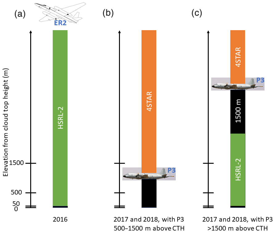
We also use partial-column AOD observed upward from the P3 with a sun photometer (Fig. 1b, c). The Spectrometer for Sky-Scanning, Sun-Tracking Atmospheric Research (4STAR) measures hyper-spectral direct solar beam. Calculated AOD is reported at 1 Hz. Our analysis excludes data with possible influences of clouds above the instrument. Further details on the instrument as well as data acquisition, screening, calibration and reduction can be found in Dunagan et al. (2013), Shinozuka et al. (2013) and LeBlanc et al. (2020).

For 2017 and 2018, we examine a combination of the 4STAR and HSRL-2 AODs, in order to cover the free troposphere both upward and downward from the aircraft that flew in it (Fig. 1b, c). The vertical coverage is compromised by two limitations intrinsic to the lidar measurements. First, the CTH is not sought within 500 m of the instrument (not to be confused with the ∼50 m lower buffer for the extinction integral). This means that the flight segments with clouds so close to the aircraft enter our analysis only if the clouds extended as deep as to reach 500 m away from it. This is at most a minor fraction of the data, as the fraction with the CTH within 550 m of the P3 altitude is a mere 3 %. Second, because of the 1500 m upper buffer for the P3-borne HSRL-2 extinction integral, we only have 4STAR above-P3 AOD for the flight segments when the plane was 500–1500 m above the CTH (Fig. 1b). We add the HSRL-2 AOD to the 4STAR AOD only for the flight segments when the P3 was >1500 m above the CTH (Fig. 1c).

For 2016, we examine the ER2-borne HSRL-2 AOD only, because with the lidar above the troposphere, two of the missing layers can safely be ignored, leaving the ∼50 m lower buffer as the only missing layer (Fig. 1a). We refer to all these AODs from the three campaigns collectively as AOD_ct (see Table 1). The wavelength dependence expressed as Ångström exponent is calculated for 10 s periods with AOD_ct at 355 and 532 nm both exceeding 0.1.

In situ aerosol instruments operated from the P3 include a nephelometer (TSI model 3563) and a particle soot absorption photometer (PSAP, Radiance Research, three-wavelength version), which measure particulate light scattering and absorption, respectively. After adjustments are made for factors such as angular truncations (Anderson and Ogren, 1998) and filter interference (Virkkula, 2010) for each wavelength, extinction coefficient and single scattering albedo at 550 nm are derived for an instrument relative humidity (RH) that is typically below 40 %. See Pistone et al. (2019) and Shinozuka et al. (2019) for more details. The nonrefractory masses of submicron particles were measured by a time-of-flight aerosol mass spectrometer (Aerodyne Inc, HR-ToF AMS; DeCarlo et al., 2006). A condensation particle counter (TSI model 3010, with ΔT set to 22 ^∘C) measured the number concentration of particles larger than about 10 nm. These in situ properties refer to the air immediately outside the P3 aircraft not a vertical column. Only the in situ measurements in 2017 and 2018 at 500–1500 m above the CTH are used in this study (Fig. 1b).

2.2 Sampling

Two methods are employed for selecting subsets of the observations for analysis. In the first (Sect. 2.2.1), we bundle data from areas hundreds of kilometers wide for each of the three campaigns, in a manner as similar to the CALIOP-based study (Chung et al., 2016) as the airborne measurements allow. In the second method (Sect. 2.2.2), we pair cloudy and clear skies with more stringent spatiotemporal criteria to isolate the impact of finer-scale phenomena. Note that both methods ignore time periods for which the 532 nm backscattering product (from which the CTH product is derived) is masked at all altitudes, as well as transit flights into and out of the study area. Cases are also excluded where the CTH exceeds 3241 m. This is to be consistent with the study by Chung et al. (2016), which refers to clouds at 680 hPa or higher pressure, although we find similar results with or without this restriction.

Figure 2 The flight paths of ORACLES. The boxes for mesoscale monthly-mean sampling are superimposed.

2.2.1 Mesoscale monthly-mean sampling

This method separates profiles measured in the three campaigns into two groups: those concurrent with a presence of low-level clouds as reported by the HSRL-2 and those concurrent with an absence of any cloud detected by HSRL-2 in the column. The groups are each aggregated into grid boxes approximately 2^∘ by 2^∘, as shown in Fig. 2. This grid is adapted from Shinozuka et al. (2019) but with additional boxes for the São Tomé-based 2017 and 2018 campaigns. In total, 109 and 39 h of flight segments are selected for the cloudy and clear groups, respectively, including minor double-counting where boxes overlap.

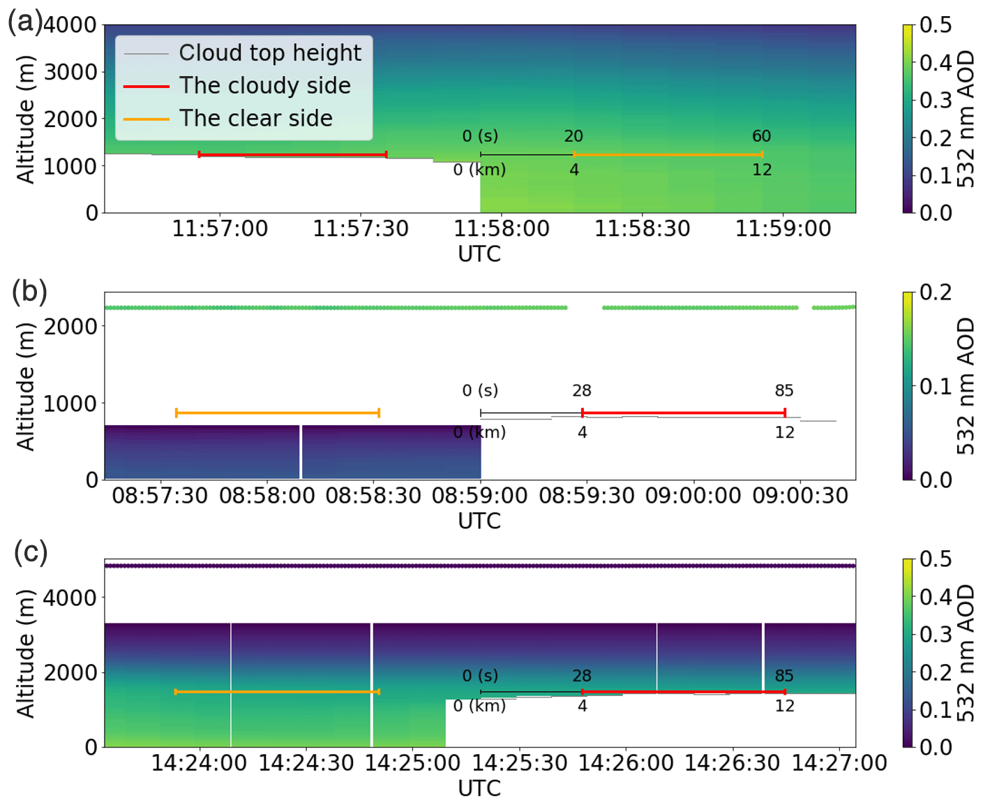
Figure 3 Examples of local-scale near-synchronous sampling, based on the HSRL-2 cloud top height (CTH) product. (a) In this subset of the ER2 flight on 12 September 2016, a cloud edge is found at 11:57:56 (denoted by 0 s and 0 km). The cloudy and clear sides, each with horizontal separation of 4–12 km measured from cloud edge, are marked by red and orange lines, respectively. The HSRL-2 AOD profiles are given for altitudes from ∼50 m above the clouds (as in Fig. 1a). (b) With the P3 500–1500 m above the CTH (Fig. 1b), as is the case with this example from 5 October 2018, we use 4STAR AOD only. The 4STAR AOD is indicated at the P3 altitudes just above 2000 m but refers to all altitudes above them. (c) With the P3 aircraft >1500 m above the CTH (Fig. 1c), as is the case for this example from 12 August 2017, the 4STAR AOD, indicated at the P3 altitudes just under 5000 m, is added to the HSRL-2 AOD at ∼50 m above the CTH. The upper limit of the integral of extinction is 1500 m below the P3 altitude.

The arithmetic mean of the CTH of the cloudy group is calculated for each day for each box, and 50 m above it is set as the lowest altitude for computing AOD_ct for each 10 s period (Sect. 2.1). Then the arithmetic mean and standard deviation are calculated for the AOD_ct, as well as other measurements (Sect. 2.1, Table 1), for each group and each box. We exclude the boxes with fewer than 10 counts of 10 s averages and the time periods with mid- and high-level clouds and operational issues. And 49 and 26 h of the AOD_ct measurements enter the analysis for cloudy and clear-sky groups, respectively.

2.2.2 Local-scale near-synchronous sampling

This method identifies cloud edges and demarcates the cloudy side and clear side of each edge based on the time series of the CTH detected by HSRL-2 for level flight legs only. Cloud edges are defined by the points in time when a cloud is detected in a profile adjacent to a profile with no cloud detection.

A clear sky and a cloud are represented by the time period of a certain length, 60 s in the example illustrated in Fig. 3a, preceding each edge and the same length following it. To ensure that clear skies and clouds are not interrupted for the length, we exclude edges for which another one is found within the length. The longer the length, the smaller the number of cloudy–clear pairs, because longer continuous clouds and clear skies are rarer. Furthermore, we set another length, say 20 s, to exclude immediately before and after the edge in order to reduce ambiguity associated with a gradual transition from cloud droplets to unactivated particles, the so-called twilight zone (Koren et al., 2007; Schwarz et al., 2017; Várnai and Marshak, 2018). We convert the temporal dimensions into horizontal ones using the mean true horizontal aircraft speed, which are 200 m s⁻¹ for the ER2 (Fig. 3a) and 140 m s⁻¹ for the P3 (Fig. 3b and c).

While Fig. 3a has one set of maximum and minimum limits of separation noted as an example, we alter them in order to assess scale dependence and sampling error as much as our airborne data permit. The way the edges are identified ensures that a measurement cannot be counted more than twice for a given range of separation. A measurement can, however, enter multiple ranges of separation. For example, a measurement 4–6 km away from a cloud edge enters the ranges of 0–6, 2–6, 2–12, 4–12, 4–20 km, and so on. In total, 5.0 h of horizontal flight are selected, including the double-counting for a given range but excluding the multiple-counting over multiple ranges. Exactly half of them are over clouds. Note that these expressions of separation are only notional; we discuss this in Sect. 4.

As with the mesoscale monthly-mean sampling, we take the arithmetic mean of the CTH of the cloudy side and add 50 m (red lines in Fig. 3). The height is extended to the adjacent clear sky (orange lines) for the calculation of AOD_ct (Sect. 2.1). The in situ measurements (Sect. 2.1, Table 1) are each averaged over the cloudy sides and over the clear sides. Cases where aerosol measurements are unavailable for 33 % or more of the time period, e.g., due to calibration or operation problems, are excluded. This makes the number of cloudy–clear pairs vary from property to property for a given range of separation. In total, 3.8 h of AOD_ct measurements enter the analysis.

2.3 Statistical hypothesis testing

We employ the paired t test, also called paired-samples t test or dependent t test, to determine whether the mean difference in each property, x (e.g., AOD_ct), between the presence and absence of low-level clouds is statistically consistent with the null hypothesis of zero difference. The procedure entails calculating the t statistic: the ratio of the mean cloudy–clear differences to their standard error, E.

$$\begin{array}{}\text{(1)}& {\displaystyle }t=\stackrel{\mathrm{‾}}{\mathrm{\Delta }x}/E,\text{(2)}& {\displaystyle }E=\mathit{\sigma }/\sqrt{N}.\end{array}$$

Here the standard error is the standard deviation computed for N−1 degrees of freedom, σ, divided by the square root of N, where N is the number of sample pairs. Note that the standard deviation is close to the root-mean-square deviation (RMSD) for small absolute mean difference unless N is smaller than five.

For the calculated t statistic, the two-tailed p value is looked up. Small p values are associated with large t statistics and hence generally large mean differences relative to RMSD. If the p value is smaller than 0.05, we reject the null hypothesis. If it is greater, we do not.

The procedure makes several assumptions. One is independence of the differences. Synoptic- and mesoscale phenomena prevalent throughout ORACLES (e.g., subsidence and anticyclones) reduce the independence of the samples. The low day-to-day meteorological variability and repeated flight paths might mean that the same aerosol–cloud conditions were sampled day after day. It is unclear whether this would reduce the independence of the cloudy–clear differences – a potential, seemingly untestable, caveat for the mesoscale monthly-mean sampling (Sect. 2.2.1). In the local scale the exclusion of contiguous cloud edges (Sect. 2.2.2) should attain a high level of independence from one another. The procedure also assumes continuous (not discrete), approximately normally distributed data that are free of outliers.

Figure 4 The mesoscale monthly-mean samples of the AOD above cloud top height. Each marker represents the mean over a box shown in Fig. 2. The bar represents the ±1 standard deviation range. The marker size is proportional to the number (n) of 10 s measurements, the fewer of the cloudy and clear groups, for each combination of box and month. N refers to the number of monthly box means with n≥10 in both cloudy and clear cases.

3 Results

The mesoscale monthly-mean method finds little systematic difference in 532 nm AOD_ct (Fig. 4). Most markers lie near the 1:1 line. The mean difference, an indicator of systematic differences, is +0.01. This is only +9 % of the RMSD, an indicator of the total (random and systematic) variability. The p value from the paired t test is 0.54. Thus, the AOD above low-level clouds is not significantly different from that at the same heights above nearby clear skies in this scale. The p value is also greater than 0.05 for log₁₀ of AOD_ct; this is something we tested just to confirm that our conclusions do not depend on the choice of linear or log scale. The same goes for the Ångström exponent and in situ aerosol properties (Table 2, see the rows labeled “Box means”). The only exception is the organic mass with a p value just under 0.05 (before rounding).

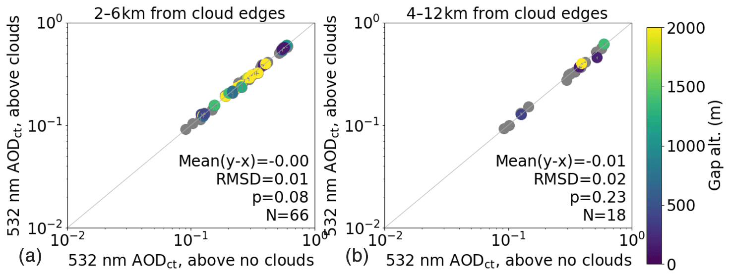
Figure 5 (a) The local-scale near-synchronous samples of the AOD above cloud top height. Each marker represents the mean over the cloudy and clear sides of a cloud edge, with each 2–6 km from the edge. The bars indicate the standard deviation of the measurements in each side, with almost all of them too short to be discernible. (b) Same as (a) except for the horizontal separation of 4–12 km.

Table 2 The mean values and the statistics on the cloudy–clear differences.

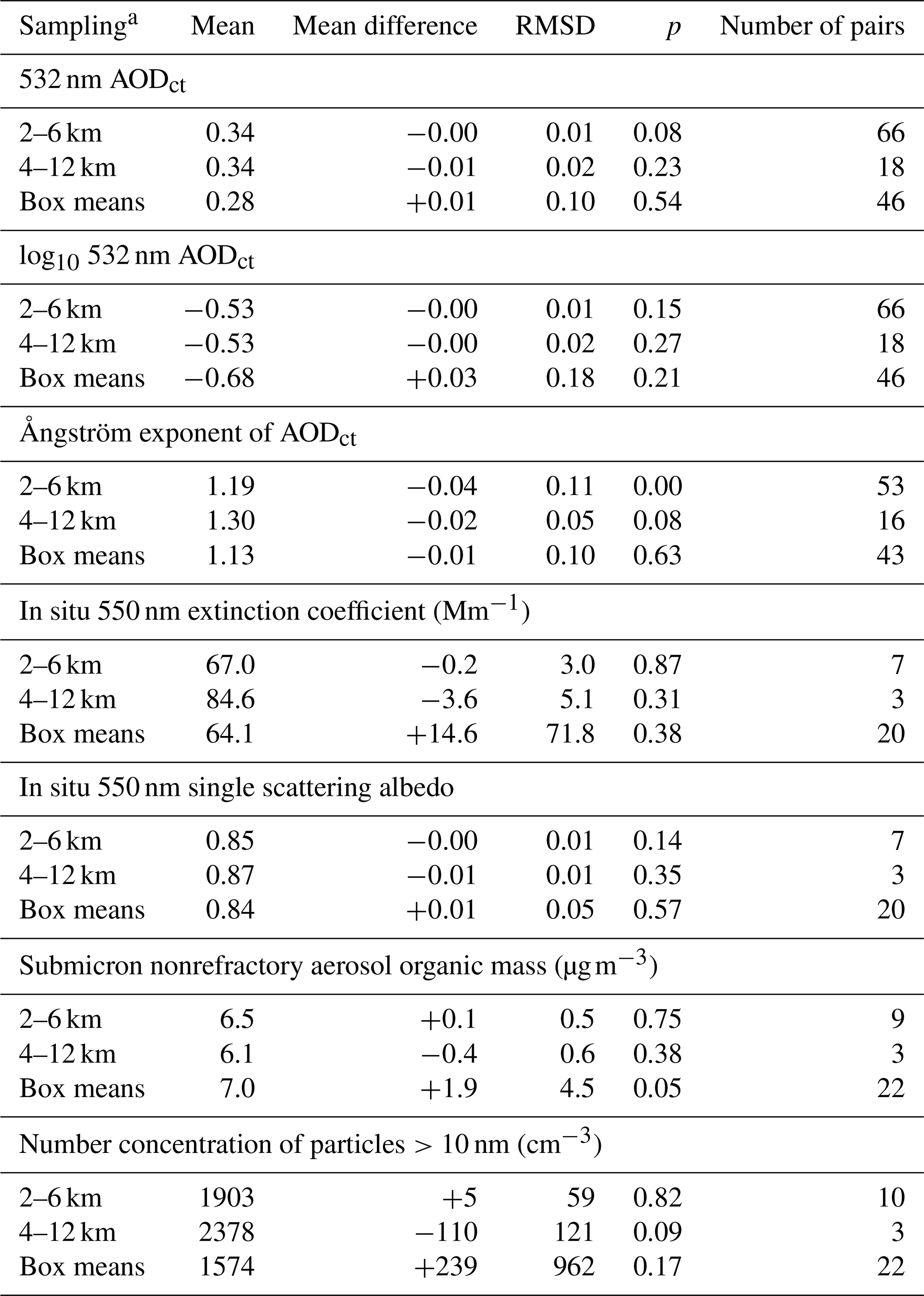
^a Either the separation from cloud edges or box means.

The local-scale near-synchronous method finds virtually the same results. The AOD_ct is compared in Fig. 5a for 2–6 km separation. The time period corresponds to approximately 10–30 s temporal range on the ER2 (13 data points from the 2016 campaign) and 14–43 s at the average P3 speed (53 from 2017 and 2018). All data points lie near the 1:1 line. The mean difference, −0.002, is only −21 % of the RMSD for 2–6 km separation. The p value is 0.08.

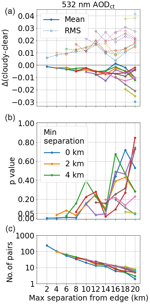
Figure 6 (a) The mean and root-mean-square deviations of the AOD above cloud top between the cloudy and clear sides of cloud edges. Each side is defined by the horizontal separation from cloud edge. The maximum separation (e.g., 12 km in Fig. 3) is indicated on the x axis. Each line represents the minimum temporal separation (e.g., 4 km in Fig. 3) of 0, 2, 4, …, 18 km in descending order of line length. (b) The p values determined through the paired t test. (c) The number of cloudy–clear pairs.

We run the same calculation for other combinations of minimum and maximum separation. Figure 6 shows the resulting statistics. The mean difference for 2–6 km separation, for example, is represented in Fig. 6a at a maximum separation (x axis) of 6 km by the solid orange line that starts after the minimum separation of 2 km. This line also shows that the mean difference is −0.01 if the maximum separation is set to 20 km while keeping the minimum at 2 km. The longest blue line represents the calculations for zero minimum separation (i.e., with the twilight zone included). All other solid lines represent the results with greater minimum separation. For example, the green line that is missing data up to 4 km indicates that the mean difference is closer to −0.01 at 12 km, as shown in Fig. 5b.

For the separation up to 20 km, the mean difference is mostly between 0 and −0.01. The p value, shown in Fig. 6b, is below 0.05 for only a handful of the ranges of separation; most of which, with minimum separation of 0–2 km, are subject to potential ambiguity associated with the so-called twilight zone (Sect. 2.2.2). Given that a p value of 0.05 simply means that there is a 1 in 20 chance that the null hypothesis is correct, we expect some low p values just by chance as we conduct many comparisons. The scarcity of low p values is also evident for log₁₀ of AOD_ct, the Ångström exponent and in situ aerosol properties including the organic mass (Table 2). Large p values are also found for the ER2- and P3-borne measurements separately and for the 4STAR and the HSRL-2 AOD separately for 2017 and 2018.

4 Discussion and conclusions

Virtually no systematic differences in aerosol properties are found between the air above low-level clouds and that above nearby clear areas in ORACLES daytime airborne measurements. The finding holds for a range (0–20 km) of distances between, and expanses of, the two air masses. Note that the temporal and horizontal dimensions associated with the local-scale near-synchronous sampling must be collectively overestimated, because the aircraft may have been running parallel to cloud edge. There is no easy way to know how far from the nearest cloud edge the airplane was in reality. Images from cameras on the plane and satellites may give some context. But we stop short of examining them, due to the perceived difficulty in unifying the definition of cloud edges between the cameras and the lidar, among other image processing issues. Although we do not know what the real distances and expanses are, that probably does not matter for the region and season of our study, judging by the consistently large p values across the notional distances and expanses. The mesoscale monthly-average sampling, relying on a larger dataset, provides consistent results. We note that this conclusion may or may not apply to environments elsewhere, especially those with less uniform clouds.

Our analysis does not support aerosol–cloud interactions, circulation patterns or anything else as a cause for a significant systematic difference in aerosol amounts; this is simply because such a difference is not evident. The lack of obvious sensitivity to the smoke–cloud gap height, indicated by marker color in Fig. 5, is consistent with this conclusion. The smoke bottom height minus the mean CTH gives an estimate of whether aerosols may be physically in contact with clouds and therefore if there is a chance of wet removal or cloud processing. Our analysis does not detect any sign of local aerosol removal by the underlying clouds.

An important difference between the present analysis and the CALIOP-based one (Chung et al., 2016), apart from the spatiotemporal range and resolution, is that the HSRL algorithm does not use any explicit layer detection (Hair et al., 2008). The return signal in the molecular signal provides a measure of the aerosol attenuation and extinction. A very tenuous aerosol layer still produces a reported extinction with a reported error bar. If the aerosol extinction is very small, the error bar may exceed the retrieved value, but there is no cutoff at small values that produces the kind of bias one gets from a detection threshold. Furthermore, the S∕N ratio is higher than that of CALIOP, and no assumptions about lidar ratio are made, as explained in Sect. 2.1.

We posit that the systematic differences between above-cloud and clear-sky AODs shown in Chung et al. (2016) are solely a CALIOP retrieval artifact, at least for the ORACLES region and season. As described in Sect. 1, the CALIOP standard algorithm has a detection bias that leads to greater AOD underestimates over clouds than in clear skies by day due to upward sunlight reflection. The authors emphasize that this bias might explain their results, pointing to a day–night contrast as evidence: “a corresponding difference cannot be seen in the ΔAOD_ct derived from nighttime retrievals [which are free of sunlight reflection]”. The present study corroborates this hypothesis, by rejecting the other possible explanations related to aerosol amounts.

We should note that the detection bias due to a low S∕N ratio is not the only known source of error in the daytime CALIOP standard AOD product. The error can also originate from a misclassified aerosol type and, hence, an incorrectly assumed lidar ratio in the CALIOP algorithm. Such an aerosol misclassification can either over- or underestimate CALIOP AOD, unlike an undetected aerosol layer. Misclassification and low S∕N ratio, taken together, explain the absence of a significant bias between CALIOP and HSRL-1 above-cloud AODs in a low aerosol-above-cloud environment such as over North America in Kacenelenbogen et al. (2014). On the other hand, Liu et al. (2015) describe a CALIOP standard daytime AOD underestimate above clouds over two regions of high above-cloud AODs. While both misclassification and low S∕N ratio are at play, Liu et al. (2015) mainly explain the CALIOP above-cloud AOD underestimate by a low S∕N ratio (especially when solar light is reflected on the underlying cloud) in the case of smoke in southeast Atlantic and an underestimate of the lidar ratio in the case of Saharan dust (see their Table 2).

In Chung et al. (2016), the lower daytime CALIOP AOD above clouds can be explained mainly by CALIOP's low S∕N ratio as there is no reason to believe that CALIOP would show a different classification bias above clouds compared to nearby clear skies. The depolarization ratio method by Hu et al. (2007) retrieves above-cloud AOD from CALIOP without a layer detection algorithm. This method may lead to a different result from Chung et al. (2016). A future study based on the Hu et al. (2007) method and extended to the globe as in Kacenelenbogen et al. (2019) will also address environments under a wider variety of synoptic- and mesoscale conditions that produce specific opaque water clouds.

Going back to the present aircraft-based study, the absence of systematic differences is good news, because satellite retrievals and studies of radiative effects do not need to treat these two conditions as different. Our results on AOD_ct justify, for example, temporal and horizontal extrapolation of above-cloud AOD to adjacent clear skies and attribution of the difference from full-column AOD to the planetary boundary layer. Our results on the aerosol intensive properties suggest that a single set of aerosol models can be used for the aerosols in the free troposphere regardless of whether clouds exist below, which may better characterize the underlying clouds and the radiative effects (Matus et al., 2015; Meyer et al., 2015). It seems reasonable to use aerosol properties retrieved in clear skies for estimating the direct radiative effects of aerosols above nearby clouds, as in Kacenelenbogen et al. (2019). But challenges remain. Random variability in AOD and other aerosol properties is significant, as indicated by RMSD in the present study and quantified for smoke elsewhere (Shinozuka and Redemann, 2011). It may be problematic to assume the same values for intensive properties for reasons not investigated here, e.g., form of combustion, degree of aerosol aging and influence of the boundary layer. These may be tackled more effectively by combining sensors of various capabilities with improved spatiotemporal resolution and retrieval algorithms (National Academies of Sciences, Engineering, and Medicine, 2018). These improved satellite observations of aerosol properties in clear skies and above clouds are urgently needed to reduce the uncertainty in total aerosol radiative forcing. For this, we are looking forward to the next generation of spaceborne lidars, radars, microwave radiometers, polarimeters and spectrometers such as the ones that will address joint Aerosol and Cloud, Convection and Precipitation (ACCP) science goals and objectives (https://science.nasa.gov/earth-science/decadal-accp, last access: 31 August 2020).