A dedicated flask sampling strategy developed for Integrated Carbon Observation System (ICOS) stations based on CO₂ and CO measurements and Stochastic Time-Inverted Lagrangian Transport (STILT) footprint modelling

In situ CO₂ and CO measurements from five Integrated Carbon Observation System (ICOS) atmosphere stations have been analysed together with footprint model runs from the regional Stochastic Time-Inverted Lagrangian Transport (STILT) model to develop a dedicated strategy for flask sampling with an automated sampler. Flask sampling in ICOS has three different purposes, namely (1) to provide an independent quality control for in situ observations, (2) to provide representative information on atmospheric components currently not monitored in situ at the stations, and (3) to collect samples for ¹⁴CO₂ analysis that are significantly influenced by fossil fuel CO₂ (ffCO₂) emission areas. Based on the existing data and experimental results obtained at the Heidelberg pilot station with a prototype flask sampler, we suggest that single flask samples are collected regularly every third day around noon or in the afternoon from the highest level of a tower station. Air samples shall be collected over 1 h, with equal temporal weighting, to obtain a true hourly mean. At all stations studied, more than 50 % of flasks collected around midday will likely be sampled during low ambient variability (<0.5 parts per million (ppm) standard deviation of 1 min values). Based on a first application at the Hohenpeißenberg ICOS site, such flask data are principally suitable for detecting CO₂ concentration biases larger than 0.1 ppm with a 1σ confidence level between flask and in situ observations from only five flask comparisons. In order to have a maximum chance to also sample ffCO₂ emission areas, additional flasks are collected on all other days in the afternoon. To check if the ffCO₂ component will indeed be large in these samples, we use the continuous in situ CO observations. The CO deviation from an estimated background value is determined the day after each flask sampling, and depending on this offset, an automated decision is made as to whether a flask shall be retained for ¹⁴CO₂ analysis. It turned out that, based on existing data, ffCO₂ events of more than 4–5 ppm that would allow ffCO₂ estimates with an uncertainty below 30 % were very rare at all stations studied, particularly in summer (only zero to five events per month from May to August). During the other seasons, events could be collected more frequently. The strategy developed in this project is currently being implemented at the ICOS stations.

1 Introduction

Since the pioneering work by Charles David Keeling who, already in the 1950s, started continuous monitoring of atmospheric carbon dioxide concentrations at the South Pole and Mauna Loa (Brown and Keeling, 1965), global coverage of continuous greenhouse gas (GHG) observations has considerably improved (https://gaw.kishou.go.jp, last access: 20 September 2020). However, there still exist large observational gaps in remote marine and continental regions of the globe, which have partly been filled by regular flask sampling and analysis in central laboratories. If frequently conducted, data from flask sampling in the marine realm are often representative of the large-scale distribution of GHGs in the atmosphere and, thus, suitable for estimating large-scale flux distributions by inverse modelling. The situation is more difficult when it comes to representative flask sampling at continental sites because there the distribution of sources and sinks is much more heterogeneous and variable than over the oceans.

In the last few decades, observational networks have been extended to the continents in order to closely monitor GHG concentrations and quantify terrestrial GHG sources and sinks. These heterogeneous terrestrial fluxes are often less well implemented in models compared to ocean fluxes (Friedlingstein et al., 2019). As biogenic sources and sinks are strongly influenced by regional climatic variability, only continental observations can provide insight into the associated ecosystem processes (Ciais et al., 2005; Ramonet et al., 2020). Besides monitoring the terrestrial biosphere, measurements over continents are also conducted to observe anthropogenic emissions, in particular from fossil fuel burning and agriculture. Due to their proximity to these highly variable sources and sinks, measurements over continents are best conducted continuously with in situ instrumentation at a high temporal resolution. Only continuous observations can resolve the variability and fully represent the entire footprint of a station (e.g. Andrews et al., 2014). However, not all atmospheric trace components we are interested in can be precisely measured in situ at remote stations yet. The most prominent example is radiocarbon (¹⁴C) in atmospheric CO₂, a quantitative tracer that separates the fossil fuel from the biospheric component in recently emitted CO₂ from continental sources (e.g. Levin et al., 2003). Note that in industrialised and highly populated areas of midlatitudes in the Northern Hemisphere, i.e. in North America, eastern Asia, or Europe, atmospheric signals from the biosphere and from fossil fuel sources are of same order (see Sect. 4.3.1). To correctly interpret absolute CO₂ concentration variations in terms of source and/or sink attribution, separation of the fossil fuel from the biogenic CO₂ signal is, therefore, mandatory. Precise ¹⁴CO₂ measurements are, however, currently only possible in dedicated laboratories and on discrete samples.

In Europe the Integrated Carbon Observation System research infrastructure (ICOS RI; https://www.icos-cp.eu/, last access: 20 September 2020) has been established to monitor GHG concentrations and fluxes in the atmosphere, in various ecosystems, and over the neighbouring ocean basins. ICOS atmosphere has set up a pan-European network of preferentially tall tower stations located at least 50 km away from industrialised and highly populated areas. The primary purpose is to monitor biogenic sources and sinks in Europe and monitor their behaviour under changing climatic conditions. In addition to continuous CO₂, CH₄, and CO observations, a subset of stations (Class 1 stations) perform 2-week integrated sampling of CO₂ for ¹⁴C analysis. Class 1 stations are additionally equipped with an automated flask sampler dedicated to three major objectives. First, the collected flasks shall provide an independent quality control (QC) for the continuous in situ measurements of CO₂, CH₄, CO, and further species mole fractions. Second, flasks shall be collected for the analysis of additional trace components not measured in situ at the stations; finally, flasks with a potentially elevated fossil fuel CO₂ component originating from anthropogenic sources in the footprint of the stations shall be analysed for ¹⁴CO₂.

Dedicated sampling strategies had to be developed for ICOS which best meet these three objectives and which can be accomplished in the framework of the infrastructure and its available capabilities and resources. This includes technical constraints at the stations but also analysis capacity at the ICOS Central Analytical Laboratories, which are analysing all flask samples in ICOS. The ICOS flask sampling strategy might change in the future, e.g. when real-time GHGs or footprint prediction tools become available.

In the current paper, we first give an introduction to the current ICOS atmosphere station network and then present a strategy for how to collect the flask samples for ICOS in a simple and cost-effective way. The sampling strategies have been developed based on footprint model simulations with a regional transport model, the Stochastic Time-Inverted Lagrangian Transport (STILT) model (Lin et al., 2003), that was implemented at the ICOS Carbon Portal (https://www.icos-cp.eu/about-stilt, last access: 20 September 2020) for ICOS station principal investigators (PIs) and data users. The first tests to develop a strategy for the quality control objective were performed at the ICOS pilot station in Heidelberg, where ICOS instrumentation and a prototype of the ICOS flask sampler have been installed, and at the Hohenpeißenberg station. The strategy was further tested for its feasibility based on the first years of continuous ICOS CO₂ and CO observations available at the ICOS Carbon Portal (ICOS RI, 2019).

2 The atmosphere component of the ICOS research infrastructure

2.1 The atmosphere station network and its Central Facilities

The ICOS atmosphere station network currently consists of 25 officially labelled stations (with 12 stations still to come), located in 12 countries, and covering Europe from Scandinavia to Italy and from Great Britain to the Czech Republic (see Fig. 1). The preferred station types are tall tower sites, allowing vertical profile sampling at a minimum of three height levels up to at least 100 m above ground level (a.g.l.). Tall tower stations cover footprints of several tens to hundreds of kilometres of distance from the sites (Gloor et al., 2001; Gerbig et al., 2006). Although their representation in state-of-the-art regional atmospheric transport models is more difficult than in the case of tower observations, due to their often long history of GHG measurements, a number of mountain and coastal stations are also part of the ICOS network. However, the flask sampling strategy developed here was designed specifically for the standard ICOS tall tower stations.

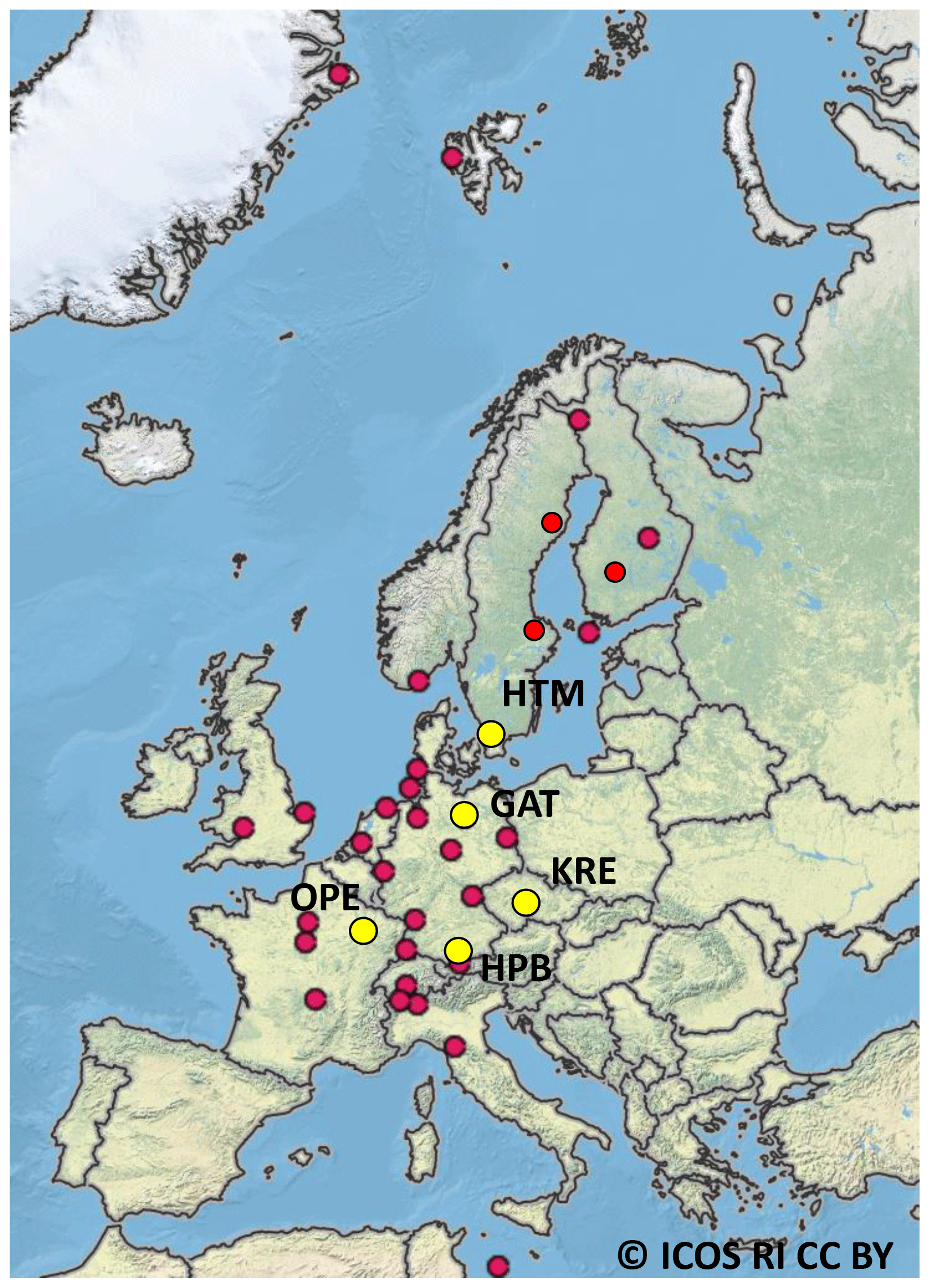
Figure 1 Map of ICOS atmosphere stations. The five stations included in this study are marked with big yellow dots: HTM – Hyltemossa, GAT – Gartow, KRE – Křešín, OPE – Observatoire Pérenne de l'Environnement, and HPB – Hohenpeißenberg. Sources: ESRI, US National Park Service and ICOS Carbon Portal.

All ICOS atmosphere stations are equipped with commercially available instruments measuring CO₂, CH₄, and CO continuously at high temporal resolutions. Instruments are tested at the Atmosphere Thematic Centre (ATC), an ICOS Central Facility hosted by the Laboratoire des sciences du climat et de l'environnement (LSCE) in Gif-sur-Yvette, France, before they are installed at the sites (Yver Kwok et al., 2015). The calibration gases for the in situ measurements are prepared and calibrated at the Flask and Calibration Laboratory (FCL), which has been established at the Max Planck Institute for Biogeochemistry in Jena, Germany, as part of the ICOS Central Analytical Laboratories (CAL). This procedure guarantees the best possible compatibility of observations within the ICOS atmosphere network and maintains the link to the internationally accepted World Meteorological Organization (WMO) calibration scales. In addition, the FCL analyses the flasks with a focus on QC and additional species. Precise ¹⁴CO₂ analysis of integrated samples and selected flasks is conducted in the second part of ICOS CAL at the Heidelberg University Institute of Environmental Physics in the Karl Otto Münnich Central Radiocarbon Laboratory (CRL).

All raw data (level 0) are automatically transferred, on a daily basis, from the measurement sites to the ATC, where they are converted to calibrated (level 1) concentration values (Hazan et al., 2016) based on regular on-site calibrations and FCL-assigned calibration values. For ongoing automatic data quality assurance of all measurements, the ATC has developed automatic procedures. Further software tools are made available by the ATC for mandatory validation of all raw data by the station PIs. These quality-assessed data form the basis of the hourly mean concentrations, which are finally released as level 2 data and made available to the user community on the ICOS Carbon Portal hosted by Lund University, Sweden. For the latest data release, see ICOS RI (2020a).

Two station types are currently implemented in the ICOS atmosphere station network, namely Class 1 and Class 2. Class 1 stations are equipped with the complete instrumentation, including integrated ¹⁴CO₂ and flask sampling. Class 2 stations perform only in situ continuous measurements of CO₂, CH₄, and CO (currently not mandatory) but with the same instrumentation and demand for data quality as Class 1 stations. A detailed description of the specifications of the instrumentation is given in the ICOS Atmosphere Station Specification document (ICOS RI, 2020b), which is regularly updated. To become an official part of the ICOS atmosphere station network, stations have to undergo a two-step labelling process, which warrants their conformance with the ICOS station specifications, including smooth data transfer to the ATC and meeting ICOS data quality requirements.

2.2 Description of selected ICOS stations

To develop and test our flask sampling strategy, we selected five ICOS Class 1 tall tower stations in four different countries. A short description of these stations is given in the following.

Hyltemossa (HTM) is located a few kilometres south of Perstorp in northwestern Skåne, Sweden (56.098^∘ N, 13.418^∘ E; 115 m above sea level – a.s.l.). It hosts a combined atmosphere and ecosystem station labelled, respectively, as Class 1 and Class 2 sites in its respective networks. The site was established in 2014 in a 30-year-old managed Norwegian spruce forest. More than 600 m away from the tower there is a mosaic consisting of forests, clear-cuts, and farm fields. Within a radius of 100 km, the elevation changes from 0 to 200 m a.s.l., while in the near vicinity of the tower the elevation gently changes by only 35 m. In the larger footprint, the site is surrounded by cities; i.e. Halmstad to the north (70 km; 58 000 inhabitants), Kristianstad to the east (45 km; 36 000 inhabitants), Lund (45 km; 111 000 inhabitants), Malmö (60 km; 318 000 inhabitants), and Copenhagen (in Denmark; 70 km; 1 990 000 inhabitants) to the southwest, and Helsingborg (45 km; 124 000 inhabitants) and Helsingør (in Denmark; 55 km; 61 000 inhabitants) to the west. The station is equipped with a Picarro, Inc. G2401 cavity ring-down spectroscopy (CRDS) gas analyser that measures CO₂, CH₄, and CO. Air inlets are located at 30, 70, and 150 m a.g.l. Air is sampled for 5 min from each level, where the data for the first minute after switching to the new level are discarded. Subsampling lines have installed 8 L mixing volumes that are continuously flushed with a flow rate of 2.1 L min⁻¹, resulting in a residence time of 270 s in each line. In addition, at the height of each air inlet, air temperature, relative humidity, and wind speed and direction are being measured.

The ICOS tall tower station Gartow (GAT; 53.066^∘ N, 11.443^∘ E; 70 m a.s.l.) is situated in the easternmost region of Lower Saxony, Germany, close to the river Elbe, approximately at the midpoint between Hamburg and Berlin. The surrounding area is very flat, with elevations ranging from less than 9 m a.s.l. (Elbe Valley) up to 124 m a.s.l. (at the Hoher Mechtin hill 35 km west of GAT). The land use in this area is dominated by forests and agricultural fields. The station hosts a lattice television tower operated and managed by the Deutsche Funkturm GmbH (DFMG). The closest cities are Schwerin (65 km north of the station; ca. 100 000 inhabitants), Wolfsburg (80 km south of the station; ca. 120 000 inhabitants), and Lüneburg (70 km northwest of the station; ca. 70 000 inhabitants). Air inlets are at 30, 60, 132, 216, and 341 m. A Picarro, Inc. G2301 cavity ring-down spectroscopy (CRDS) gas analyser, measuring CO₂, CH₄, and CO, and, since the beginning of 2019, a Los Gatos Research, Inc. (part no. 913-0015; Enhanced Performance – EP) off-axis integrated cavity output spectroscopy (OA-ICOS) analyser, measuring CO and N₂O, have been installed in a container next to the tower. Air is sampled for 5 min from each level, where data for the first minute after switching to the new level are discarded. All inlet lines are continuously flushed with approximately 5 L min⁻¹. Meteorological sensors for air temperature, relative humidity, and wind speed and direction have been installed at every sampling height. For historical reasons, Gartow modelling was conducted for 344 m a.g.l. (and not for the highest sampling level at 341 m); this difference between the measured and modelled level is, however, not relevant for the comparisons presented in the context of this study.

Station Křešín u Pacova (KRE; 49.572^∘ N, 15.080^∘ E; 534 m a.s.l.) is located in the central Czech Republic, about 100 km southeast of Prague. The site was established in 2013 close to the Košetice Observatory, a station of the Czech Hydrometeorological Institute with 30 years of practice in meteorology and air quality monitoring. Today, these two stations form the National Atmospheric Observatory in the Czech Republic. Since the site is designed as a background station, the area is not significantly influenced by human activity. The tower is surrounded by fields and, at a greater distance, forests and small villages (the closest is 1 km away). There is a highway running northeast of the tower at an approximate distance of 6 km; however, the wind frequencies from the north and east are 9 % and 5 %, respectively. The closest towns, namely Pelhřimov, Vlašim, and Humpolec, with 10 000 to 17 000 inhabitants, are located approximately 20 km away from the station. As for industrial activity, a small wood-processing company is located 20 km to the west (which is the prevailing wind direction). The town of Havlíčkův Brod, with ca. 20 000 inhabitants, is located about 30 km from the site; larger towns (up to 50 000 inhabitants) are about 40 km away (i.e. Jihlava and Tábor). Further still, there are only towns with populations of, at most, 35 000 inhabitants, except for Prague (80 km; 1 million inhabitants), Pardubice (80 km; 90 000 inhabitants), and České Budějovice (90 km; 90 000 inhabitants). The terrain around the tower is relatively flat within a few kilometres' distance, with only small hills around. The Bohemian-Moravian Highlands, where the site is located, have an average altitude of 500–600 m a.s.l., with rare spots of 800 m a.s.l. The highest hills, namely Javořice (837 m a.s.l.) and Devět skal (836 m a.s.l.), are located 43 m and 69 km away. The station is equipped with the ICOS atmosphere-recommended instrumentation for CO₂ and CH₄ (Picarro, Inc. G2301 CRDS) and for N₂O and CO (Los Gatos Research, Inc.; part no. 913-0015; EP). The air is sampled at 10, 50, 125, and 250 m levels of the tower. Sampling period is 10 min per height, where the highest level is sampled in between all other levels. This results in a complete vertical profile measured within 1 h, with a preference for the 250 m level. After switching to a new height, 3 min measurements are always excluded (known as the stabilisation period). All sampling heights of the tower are equipped with meteorological sensors (wind speed and direction, air pressure and temperature, and relative humidity).

The Observatoire Pérenne de l'Environnement (OPE; 48.563^∘ N, 5.506^∘ E; 395 m a.s.l.) is located on the eastern edge of the Paris basin in the northeastern part of France. The station is located in a rural area with large crop fields, some pastures, and forest patches. A local village and small roads are about 1 km away. The closest large towns are between 30 and 40 km away, and a major road is found at a distance of about 15 km. The station hosts a complete set of in situ measurements of meteorological parameters, trace gases (CO₂, CH₄, N₂O, CO, O₃, NO_x, and SO₂), and particle characteristics. The station is part of the French aerosol in situ network, contributing to Aerosol, Clouds and Trace Gases Research Infrastructure (ACTRIS; https://www.actris.eu/, last access: 20 September 2020) and the Institut de Radioprotection et de Sûreté Nucléaire (IRSN) network for ambient air radioactivity monitoring. It also contributes to the French air quality monitoring network and to the European Monitoring and Evaluation Programme (EMEP). The infrastructure, including a 120 m tall tower, was built in 2009–2010, and the various measurements started between 2011 and 2013. Ambient air is sampled at three levels, namely 10, 50 and 120 m a.g.l., of the tower and is analysed by Picarro, Inc. cavity ring-down spectrometers (CRDSs; series G1000 and G2000) for CO₂, CH₄, H₂O, and CO as well as Los Gatos Research, Inc. off-axis-ICOS spectrometers for N₂O and CO (Conil et al., 2019). The sampling period for each level is 20 min, including an automatic rejection of the first 5 min. Meteorological parameters are measured at all air sampling levels.

The ICOS station Hohenpeißenberg (HPB; 47.801^∘ N, 11.010^∘ E; 934 m a.s.l.) is located on top of a solitary hill that rises approximately 300 m above the almost flat to rolling landscape, 30 km north of the Alps and approximately 60 km southwest of Munich. The main land uses are forests and meadows. The station hosts a concrete television tower operated and managed by the DFMG. Cities closest to the station are Weilheim (10 km east of the station; 20 000 inhabitants), Landsberg (30 km north of the station; 30 000 inhabitants), Augsburg (60 km north of the station; 270 000 inhabitants), Munich (60 km northeast of the station; 1 million inhabitants), and Innsbruck (in Austria; 65 km south of the station; 127 000 inhabitants). Air inlets are at 50, 93, and 131 m. A Picarro, Inc. G2401 CRDS analyser, measuring CO₂, CH₄, and CO, and a Los Gatos Research, Inc. (part no. 913-0015; EP) OA-ICOS analyser, measuring CO and N₂O, are installed in the basement of the tower. Air is sampled for 5 min from each level, where data for the first minute after switching to the new level are discarded. All inlet lines are continuously flushed with approximately 5 L min⁻¹. Meteorological sensors (air temperature, relative humidity, and wind speed and direction) are installed at every sampling height.

2.3 Atmospheric transport modelling for ICOS stations

A footprint simulation tool based on the regional atmospheric transport model, STILT (Lin et al., 2003; Gerbig et al., 2006), was implemented at the ICOS Carbon Portal (https://www.icos-cp.eu/about-stilt, last access: 20 September 2020) as a service for ICOS station PIs and data users. The STILT model simulates atmospheric transport by following a particle ensemble, released at the measurement site, backwards in time and calculating footprints that represent the sensitivity of tracer concentrations at this site to surface fluxes upstream. The footprints are mapped on a $\mathrm{1}/\mathrm{12}{}^{\circ }$ latitude $\times \mathrm{1}/\mathrm{8}{}^{\circ }$ longitude grid and are coupled to the Emission Database for Global Atmospheric Research (EDGAR) version 4.3.2 emission inventory (Janssens-Meanhout et al., 2019) and the biosphere model, Vegetation Photosynthesis and Respiration Model (VPRM; Mahadevan et al., 2008), to simulate atmospheric CO₂ and CO concentrations. These regional concentration components represent the influence from surface fluxes inside the model domain (covering the greater part of Europe). For CO₂, the contributions from global fluxes are accounted for by using initial and lateral boundary conditions from the Jena CarboScope globally analysed CO₂ concentration fields (http://www.bgc-jena.mpg.de/CarboScope/s/s04oc_v4.3.3D.html, last access: 20 September 2020), while for CO only regional contributions are evaluated in our study. Note that STILT does not account for the stack emission height of point sources. This may cause biases when estimating ffCO₂ contributions from close-by emissions of, for example, power plants. However, as this model deficiency becomes less important with increasing distance from the source, it seems of minor relevance for the ICOS stations studied here as they are located far away from major emitters.

2.4 The automated ICOS flask sampler

The automated ICOS flask sampler was designed and constructed at the Max Planck Institute for Biogeochemistry (MPI-BGC), Jena, Germany, by the Flask and Calibration Laboratory (FCL) of the CAL to allow automated air sampling under highly standardised conditions. The sampler can hold up to 24 individual glass flasks (four drawers with six flasks each) for separate air sampling events (Fig. 2, upper panel). The glass flasks can be individually replaced and sent to the CAL for analysis. The glass flasks used within ICOS (3 L volume; product no. ICOS3000; Pfaudler Normag Systems GmbH, Germany) were developed according to ICOS' specific requirements based on well-proven designs (Sturm et al., 2004). Each flask has two valves, one at each end, that allow air exchange by flushing sample air through the flask. The flasks are attached with 1∕2 in. clamp ring connectors to the flask sampler. The flask valves, with polychlorotrifluoroethylene (PCTFE) sealed end caps, can be opened and closed by a motor.

Figure 2 Photograph of the ICOS flask sampler with a schematic flow diagram.

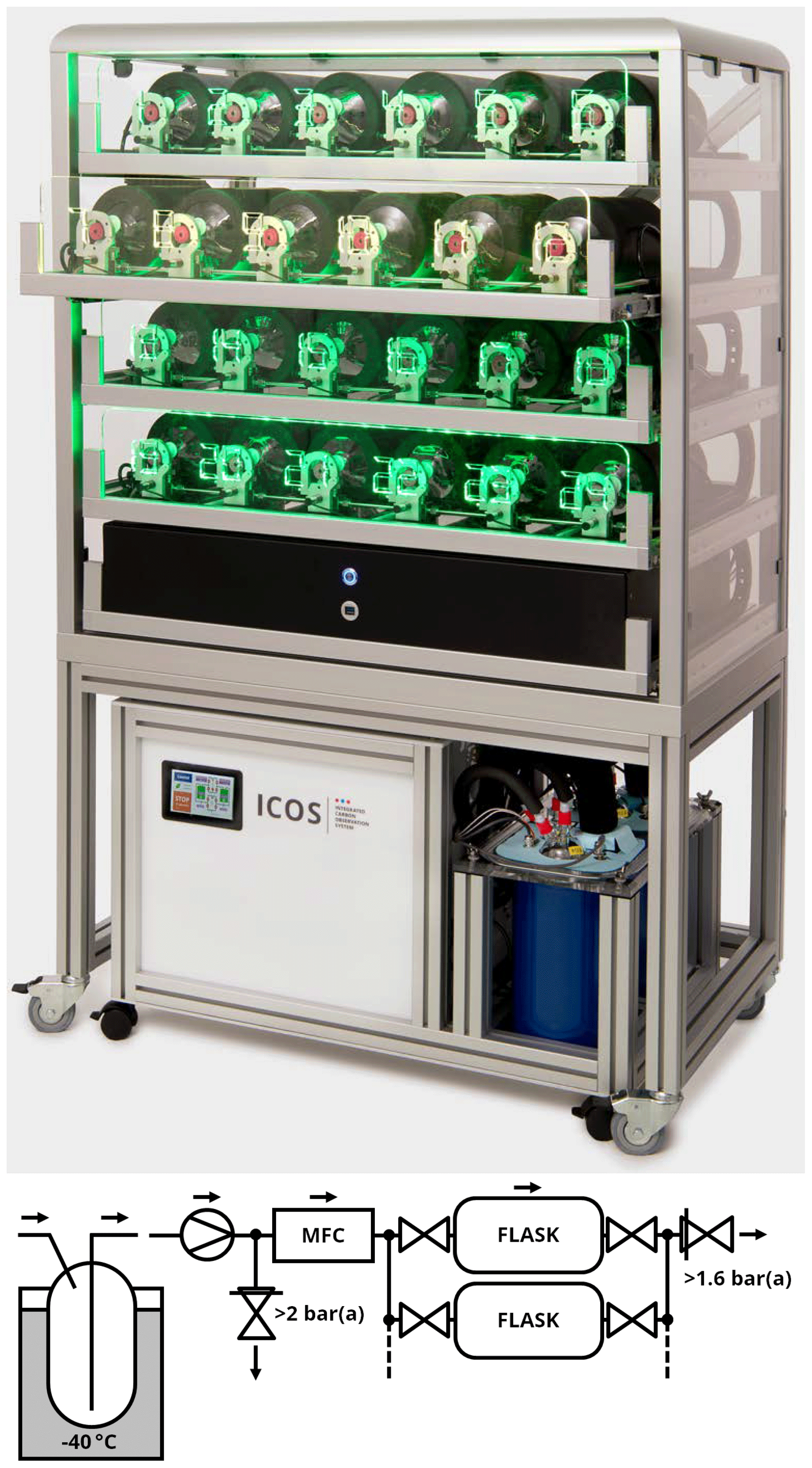
A sample is taken by flushing air through a flask at a constant overpressure of 1.6 bar (absolute). Sampling at overpressure increases the amount of available sample air for analysis and allows for the detection of flasks with leak problems. Flasks are prefilled with 1.6 bar of dry ambient air with a well-known composition at the FCL to avoid concentration changes due to wall adsorption effects. The schematic sampler layout is depicted in the flow diagram in Fig. 2. Incoming air is dried to a dew point of approximately −40 ^∘C by passing through a cooled glass vessel where the exceeding humidity is frozen out. The glass vessel is placed in a silicon oil heat bath that is cooled for drying and heated for flushing out the collected water to regenerate the trap. The drying unit is automated and consists of two independent inter-switchable drying branches that complement each other and allow a near interruption-free drying. The dryer design is inspired by an already existing system from Neubert et al. (2004). The incoming sample air is compressed with a pump (J161-AF-HJ0; Air Dimensions, Inc.). A mass flow controller (MFC; F-201CV; Bronkhorst) between the compressor and flasks allows one to sample preset flow rates; i.e. with a decreasing flow rate over time so that the sample represents a real average, for example, over 1 h (Turnbull et al., 2012). The flask pressure during sampling (1.6 bar) is kept constant through a pressure regulator at the outlet of the flasks. An overpressure valve set at 2.0 bar behind the pump assures a constant flow rate through the intake line, independent of the flow rate through the mass flow controller.

In ICOS we strive to sample real 1 h mean concentrations in 3 L flasks. The 1∕t filling approach requires, for this specific case, a theoretical dynamic flow rate between 80 mL min⁻¹ and infinity. In reality, the maximum flow rate of the selected flow controller is limited to 2 L min⁻¹. An almost constant weighting of the sample concentration over the 1 h sampling time is achieved by the temporal modulation of the sample flow f(t) (standard litre per minute – SLPM) passing a flask, which acts at the same time as mixing volume V given in litre standard temperature and pressure (STP). The flow rate f is changed over time t according to $f\left(t\right)=V/(t-t_{\mathrm{0}})$. Since the flow rate at the start time t₀ in a 1∕t function would be infinite, a 30 min flushing phase at maximum flow rate precedes the averaging period to ensure a complete air exchange in the flask with ambient air before the sampling starts.

The concentration c_F(t) in the flask is determined by the ambient air concentration c_A(t) and can be described as a time series using sufficiently small time steps Δt as follows:

$$\begin{array}{}\text{(1)}& c_{\mathrm{F}}\left(t+\mathrm{\Delta }t\right)={\displaystyle \frac{c_{\mathrm{F}}\left(t\right)\cdot \left(V-f\left(t\right)\cdot \mathrm{\Delta }t\right)+c_{\mathrm{A}}\left(t\right)\cdot \left(f\left(t\right)\cdot \mathrm{\Delta }t\right)}{V}}.\end{array}$$

The resulting weight of the ambient air concentration $w_{c_{\mathrm{A}}}$ at time step t_n in the flask depends on the following two factors:

$$\begin{array}{}\text{(2)}& w_{c_{\mathrm{A}}}\left(t_n\right)\sim c_{\mathrm{A}}\left(t_n\right)\cdot {\displaystyle \frac{f\left(t_n\right)\cdot \mathrm{\Delta }t}{V}}\cdot \prod _{i=n+\mathrm{1}}^{\mathrm{E}}\left(\mathrm{1}-{\displaystyle \frac{f\left(t_i\right)\cdot \mathrm{\Delta }t}{V}}\right),\end{array}$$

namely the weight at the moment when the ambient air portion enters the flask, and a weight-reduction factor caused by dilution with sampled air entering the flask at later times. The reduction is calculated by multiplication of the respective dilution steps from t_n to the sampling end time t_E. This weighting function has to be applied to the ambient air measurements so that the flask concentrations can be compared with the in situ data. Average in situ minus flask concentration differences with the aimed uncertainty can only be reached under sufficiently stable concentration conditions during sampling.

With the current design of the flask sampler, technical restrictions do not allow parallel sampling of flask duplicates or triplicates as a means for quality control, for example, based on flask pair agreement. The technical effort for allowing exact parallel hourly averaged sampling is very high; it would, for example, require flow controllers for all individual flasks sampled in parallel. Therefore, the ICOS Atmosphere Monitoring Station Assembly (MSA) decided to sample only single flasks. This seems appropriate because in the ICOS network the flask sampler is always collecting flasks in parallel to continuous measurements, and erroneously collected flasks, or errors due to flask leakages, can be detected when comparing results with the continuous data. Therefore, in contrast to the general practice of duplicate flask sampling, in our network single flask sampling seems to be sufficient for meeting ICOS objectives. This has the additional advantage that single flask sampling allows more frequent sampling and, thus, a more representative coverage of the footprint of the stations. If true duplicate samples are required in the future, the flask sampler is designed to accommodate an additional mass flow controller to fulfil this task. The sampler is controlled by an embedded PC offering a broad range of interaction possibilities satisfying the emerging needs within ICOS. Sampling event time schemes can be preprogrammed, and communication with external devices (i.e. data loggers) is possible with analogue or digital signals. Flask-to-port attributions are completely barcode controlled. Sampling and sensor data are automatically stored, and all necessary sampling-related data can be automatically transferred to the CAL. Various automated internet-assisted approaches, like remote programming of sampling times and preselection of samples, are possible.

3 Aims and technical constraints of ICOS flask sampling

As briefly outlined above, there are three main aims for regular flask sampling at ICOS stations:

1. Flask results are used for comparison with in situ observations (i.e. CO₂, CH₄, CO, and N₂O). This comparison provides an ongoing quality control (QC) of the in situ measurement system, including the intake lines. It is of the utmost importance that ICOS measurements meet the WMO compatibility goals (WMO, 2020) for all GHG components. Already very small biases between station data lead to erroneous source and/or sink distributions if used in model inversions (e.g. Corazza et al., 2011). Therefore, a comparison of continuous in situ data with flask data provides a very efficient QC and a basis for determining reliable uncertainties of data.

2. Flasks are analysed for components not measured continuously at the station, such as SF₆ or H₂, but also stable isotopes of CO₂ or the O₂:N₂ ratio. The aim here is to monitor large-scale representative concentration levels of these components, allowing estimations of their continental fluxes with the help of inverse modelling. Selecting, for example, only situations of low ambient variability may cause a significant bias when these data are used in inverse models for source and/or sink budgeting.

3. A subset of flasks is analysed for ¹⁴C in CO₂, allowing the determination of the atmospheric fossil fuel CO₂ component (ffCO₂) and, with help of these data and inverse modelling, estimating the continental fossil fuel CO₂ source strength of the sampled areas.

To meet aims 1 and 2, flask sampling during well-mixed meteorological conditions is required, and the sampled footprints should not be dominated by particular hotspot source areas. Particularly for aim 2, we further strive to cover the entire daytime footprint of the station. In contrast, aim 3, due to the generally small fossil fuel signals at ICOS stations, requires targeted sampling of “hotspot emission areas” in the footprint to maximise the fossil fuel CO₂ signal in the samples. Note that the detection limit (or measurement uncertainty) of the fossil fuel CO₂ (ffCO₂) component with ¹⁴CO₂ measurements is of order 1–1.5 parts per million (ppm; e.g. Levin et al., 2011).

There are a number of technical and/or logistical constraints concerning flask sampling, shipment, and analysis in ICOS which need to be taken into account when designing an operational sampling strategy that best meets the three aims listed above. The most important limitations are listed in the following:

• 1.

  Timing. In order that all flask sample results are useful for flux estimates with current regional inversion models, flasks should be collected during midday or in the early afternoon at the standard ICOS tall tower stations. During this time of the day, atmospheric mixing is strong, and model transport errors are smaller than during night (Geels et al., 2007). For all samplings, wind speeds should be larger than about 2 m s⁻¹ so that the sampled footprint is well defined. The strategy outlined below has been developed for tall tower sites that are located not directly at the coast (i.e. that are of a predominantly continental character).

• 2.

  Intake height. There is only one intake line from the highest level of the tower running to the flask sampler; therefore, only the continuous observations from this height can be quality controlled with parallel sampled flasks (aim 1). As modellers prefer using data (aim 2) from the highest level of the tower (largest footprint, most representative, etc.), all flasks will be sampled from that highest level (as specified in the ICOS Atmosphere Station Specification Document; ICOS RI, 2020b).

• 3.

  Integration period. Flasks should be sampled as integrals; i.e. the collected sample should represent a real mean of ambient air (e.g. 1 h mean, comparable to the current model resolution). Also, synchronising in situ continuous observations and integrated flask sampling is important for the quality control aim (aim 1). This latter requirement is easier to achieve with longer integration times in flask sampling. This means, however, that for comparison reasons, the continuous in situ observations must be kept at the flask sampling height during the entire flask sampling period (i.e. no calibration gas measurement, no switching of in situ intake heights during flask sampling, and no profile information available). This also means that flow rates, delay volumes, and residence times in the tubing, as well as the time of both flask and in situ sampling systems must be properly monitored.

• 4.

  Flask handling. Flasks need to be installed and removed manually from the sampler. Remote stations are regularly visited, about once per month, by a technician. The flasks sampled to meet aim 1 should be shipped to the FCL within 1 month after sampling so that a potential bias between in situ and flask analyses is detected without major delay. ¹⁴CO₂ analysis of flasks in the CRL is less urgent; therefore, a few months' delay in the shipment of flasks collected for aim 3 are acceptable.

• 5.

  CAL measurement capacity. While the capacity for flask analysis at the FCL has been designed for a total of about 100 flask analyses per station per year, the capacity for ¹⁴CO₂ analyses in the Central Radiocarbon Laboratory (CRL), which are performed after the analysis of all other components at the FCL, are only about one-quarter, i.e., on average, 25 samples per station per year. Consequently, all flasks will be shipped from the station to the FCL, and after analysis, a subset will be shipped to the CRL for further analysis. After all analyses have been finished, all flasks, including those which were analysed at the CRL, are leak-tested and conditioned at the FCL before being dispatched to the stations.

4 Results

4.1 Solutions and testing to meet aim 1: ongoing quality control

The ICOS atmosphere station network, supported by the ICOS Central Facilities (ATC and CAL), has been designed and implemented to achieve the highest possible accuracy, precision, and compatibility of atmospheric GHG measurements. For ICOS CO₂ observations, a compatibility goal of 0.1 ppm or better is compulsory. Similarly, ICOS needs to meet the WMO compatibility goals for CH₄ and CO, which are 2 parts per billion (ppb) for both gases (WMO, 2020). First evaluations of ICOS CO₂ measurements indeed yield monthly mean afternoon differences between stations in the free troposphere above 100 m of typically very few parts per million (Ramonet et al., 2020), underlining the importance of the excellent precision and compatibility of these observations.

With regular and frequent comparisons of flask and in situ measurements, ICOS aims to independently monitor their compatibility and provide respective alerts if, for example, the average difference of CO₂ exceeds 0.1 ppm over a few weeks of comparisons. Using flasks sampled from a dedicated intake line to crosscheck the in situ measurements is an important part of the ICOS quality management. It allows an independent end-to-end QC of the entire in situ measurement system consisting of inlet system, drier, analyser, and calibration. As mentioned above, for logistical reasons, about once per month, or every 5 weeks, a box with 12 flasks is scheduled to be shipped from a remote station to the FCL. After analysis, the flask results covering about 1 month of time will be compared with the corresponding in situ data. In the following paragraph, we elaborate on the minimum number of comparison flasks and the corresponding time delay for detecting a significant CO₂ bias between flask and in situ measurements larger than 0.1 ppm. Therefore, we tested the envisaged flask sampling procedure experimentally at the ICOS pilot station in Heidelberg and present here its first application at an ICOS field station.

4.1.1 Flask and in situ CO₂ comparisons in Heidelberg

Similar to the official ICOS atmosphere stations, Heidelberg is equipped with an ICOS-conforming CRDS instrument continuously measuring CO₂, CH₄, and CO in ambient air. In addition, the Heidelberg instrument is calibrated with standard gases provided by the FCL, and its continuous data are automatically evaluated at the ATC. All flasks have been analysed at the FCL. However, since the site does not have a high tower and is located in an urban environment, the variability of the signal can complicate the flask versus in situ comparison.

In order to collect a real hourly integrated air sample in the flask, the flow rate through the flask has to be adjusted during the filling process (Turnbull et al., 2012; see Sect. 2.4). First tests with a 1∕t decreasing flow rate through the flasks were conducted in Heidelberg during the period from September 2018 to February 2019 and with a better-suited flow controller for the 1∕t decreasing flow rate from May to October 2019. Ambient air, for continuous measurements and for flask sampling, was collected via a bypass from a permanently flushed intake line from the roof of the institute's building, about 30 m above local ground. These flasks were collected not only at low ambient air variability during afternoon hours but also during other times of the day when within-hour concentration variations for CO₂ at this urban site were higher than 10 ppm. The results of the concentration differences between in situ and flask measurements for CO₂ are shown in Fig. 3a and b. During the first experimental period we obtained three outliers for which the flask CO₂ results were up to more than 3 ppm higher than the in situ measurements. CH₄ and CO in the flasks (not shown) did, however, compare very well and were within a few parts per billion of the continuous in situ data. Although one of the mass flow controllers had some problems with regulating the flow over the large range of flow rates exactly, we did not find obvious reasons for the malfunction of the sampling system. The only explanation for the outliers may, thus, be the contamination of these flasks with room air, which is elevated in CO₂, but not in CH₄ or CO, compared to outside air.

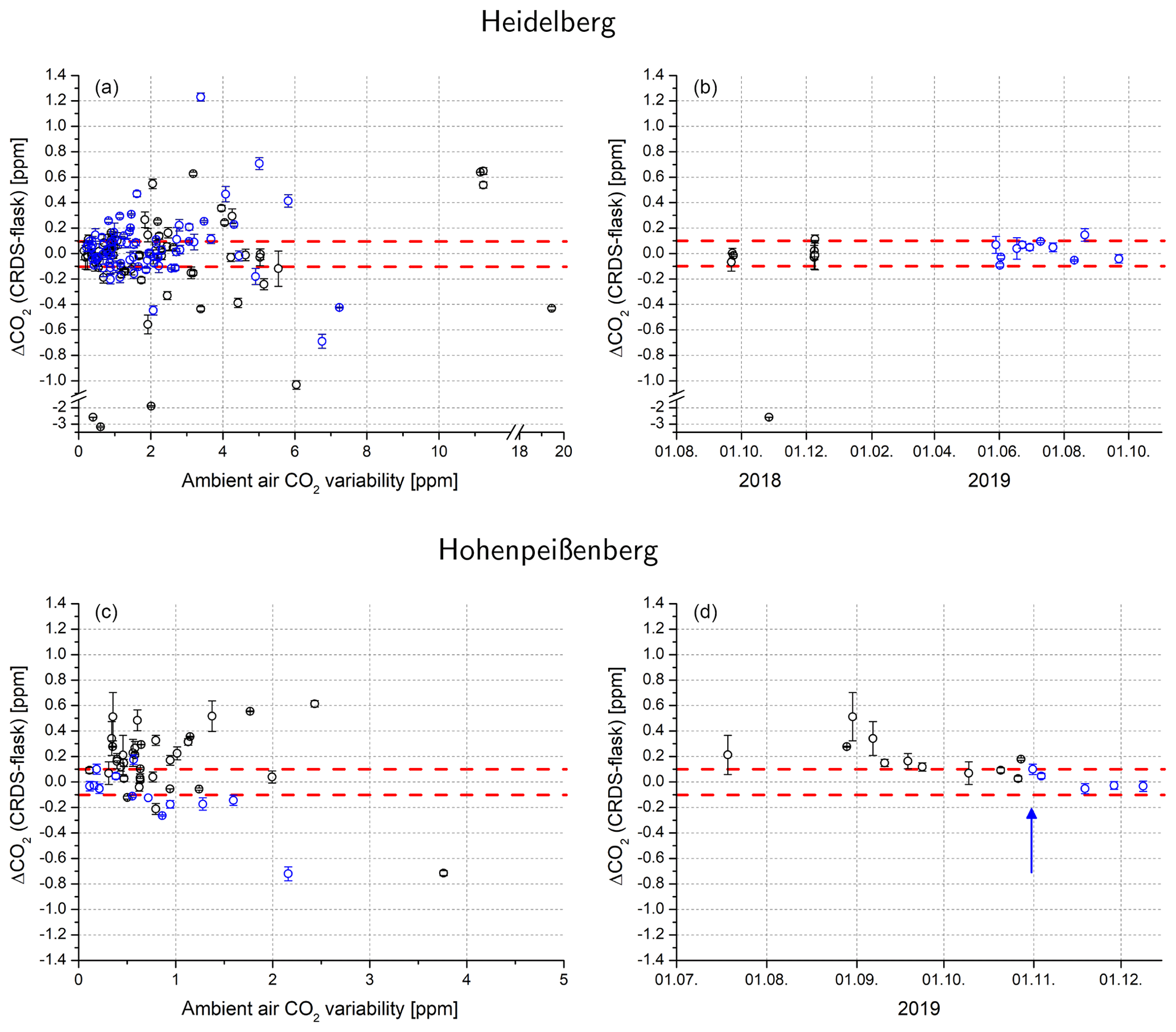
Figure 3 In situ minus flask CO₂ results obtained with the 1∕t flask flushing method to obtain a real hourly mean sample. (a–b) Results from Heidelberg; flasks from the second comparison period are marked in blue. (a) Results for all comparison flasks plotted versus ambient variability. (b) Temporal development of the in situ minus flask measurements for ambient air CO₂ variability <0.5 parts per million – ppm. All differences in the second comparison period lie within the required ±0.1 ppm compatibility range. No sampling was performed between February and May 2019. (c–d) Same as (a) and (b) but for results from Hohenpeißenberg. Flasks from the comparison period after 30 October 2019 (the date when the leak was sealed) are plotted in blue. (d) Temporal development of the in situ minus flask measurement for ambient CO₂ variability <0.5 ppm. All five differences, after sealing the leak on 30 October 2019 (blue arrow; blue dots), lie within the required ±0.1 ppm compatibility range.

If we disregard the three outliers in the first testing period (one at a low variability situation; see Fig. 3a) and consider only the observations with ambient air CO₂ variability <0.5 ppm, the limited results from the (polluted) Heidelberg site give us the confidence that the flask samples collected over 1 h at low ambient CO₂ variability are well suited for meeting our first aim (i.e. ongoing quality control at Class 1 stations). It is important, though, that the different air residence times in the intake systems of the flask sampler and in situ instrument are properly adjusted; they may significantly differ, for example, if a mixing volume system is installed in the intake lines (as at Hyltemossa). The mean differences between in situ and flask measurements for CO₂ in Heidelberg have been −0.01 ppm at an ambient CO₂ variability of less than 0.5 ppm, with a standard deviation of ±0.04 ppm (n=18); also see Fig. 3b, which shows that all 18 low variability comparisons lie within the ±0.1 ppm compatibility range indicated by the dashed red lines. For CH₄ we observed, for ambient variability smaller than ±10 ppb, a mean difference of 0.20 ppb, with a standard deviation of ±0.81 ppb (n=111). CO comparison data have not been evaluated here as the CRDS in situ data were not finally calibrated and, thus, not fully compatible with the flask results.

The test measurements in Heidelberg clearly showed that meaningful QC results can best be obtained during situations of low ambient concentration variability. Individual concentration differences increase with increasing ambient variability within the 1 h comparison period. The reason for this increase may be uncertainties in the synchronisation of the measurements (note that a few minutes of shifts in the timing of the integration already introduces a significant bias) or due to incorrect flow rates through the flasks in the 1∕t sampling scheme. For the QC aim, flask samples should preferentially be collected during low variability situations. We therefore evaluated how frequent afternoon events with less than 0.5 ppm variability occur at typical ICOS stations. In the years 2016 to 2019, except for a few stations and a few summer months, we found, at all five stations, at least 10 h per month at midday (13:00 h local time – LT) with hourly CO₂ standard deviations smaller than 0.5 ppm. On average over the year, more than half of all midday hours had CO₂ standard deviations below 0.5 ppm. Based on this evaluation, we decided that we would not need to preselect sampling days with low ambient variability but could pursue a very simple sampling scheme, e.g. sampling every 3 or 4 d, to be able to detect a mean bias larger than 0.1 ppm between flask and continuous measurements within a period of 4–5 weeks. On average, we can expect that every second flask we sample is suitable for precise intercomparison with in situ measurements. This simple methodology will help us meet aim 2 (see below).

4.1.2 Flask and in situ CO₂ comparisons at the ICOS station Hohenpeißenberg

The very first field test of our flask sampling scheme for QC was conducted at the ICOS station of Hohenpeißenberg (HPB). From the highest level of the tall tower (131 m), ambient air, for continuous measurements and for flask sampling, was collected via two separate lines. Collecting flasks at HPB started in July 2019. The flasks were always sampled with a decreasing 1∕t flow rate and sampled between 12:30 and 14:00 Coordinated Universal Time (UTC) as we aimed for conditions with low ambient variability, which occurs more frequently in well-mixed conditions during the afternoon. Up to now, 48 flasks have been collected, which could be used for the QC of this ICOS Class 1 station. The overall results of the concentration differences for CO₂ for the complete test period are shown in Fig. 3c.

Our first results of the comparison between continuous measurements and flasks were available in October 2019 and showed larger differences between in situ and flask measurements than expected. A mean difference of 0.34 ppm, with a standard deviation of ±0.13 ppm (n=4), was determined for situations with an ambient variability of less than 0.5 ppm. Based on these results, the intake system and the entire CO₂ instrumentation were carefully checked. Whilst the last regular leak test on 10 April 2019 passed the ICOS specifications, an unscheduled leak test was performed at the end of October 2019, following the unexpected flasks results. During this test, a leak in the 131 m sampling line to the instruments for the continuous measurements was detected in the shelter. The leak was eliminated on 30 October 2019, and leak tightness was confirmed by a second leak test on 19 November 2019.

For the period after the leak elimination, the calculated differences between in situ and flask measurements for an ambient variability of less than 0.5 ppm all lay within the compatibility goal for CO₂ (0.1 ppm); see blue dots in Fig. 3d. The mean difference between flasks and in situ measurements is −0.02 ppm, with a standard deviation of ±0.04 ppm (n=5). These results of the first field test of the flask sampling scheme for QC are promising, for example, for enabling the detection of potential leaks at the stations. Once the flask QC procedures have been set up operationally, potential system malfunctions can be detected within a month, complementing the half-yearly compulsory ICOS leak tests.

4.2 Solutions and testing to meet aim 2: representative flask sampling

In the preceding section we showed that low ambient variability situations would be best suited for meeting aim 1 as synchronisation and exact weighting of flask filling and in situ measurements are not so important at low ambient variability. Moreover, a potential bias between flask and in situ measurements could be detected with better confidence and with an increased number of comparisons. However, to meet aim 2, a scheme for collecting flasks only during low variability situations may cause a significant bias in the sampled footprint. We have tested if such a sampling bias would be visible in the European ICOS network and calculated, with STILT, all midday (13:00 LT) footprints of the five selected stations for the year 2017, using the Jupyter Notebook package of Karstens (2020). Figure 4 shows the respective aggregated footprints for October 2017. A time of 13:00 LT was chosen as an example throughout the paper, but other afternoon hours could also have been chosen, leading to similar results. The left column in Fig. 4 shows the aggregations if every afternoon hour (13:00 LT) was sampled, the middle column shows the aggregated footprints for every third day, and the right column shows the 10 footprints with the lowest variability during October 2017. As expected, the regional coverage of the entire station footprint is generally better when sampling randomly, every third day, than when sampling on the 10 d with the lowest variability.

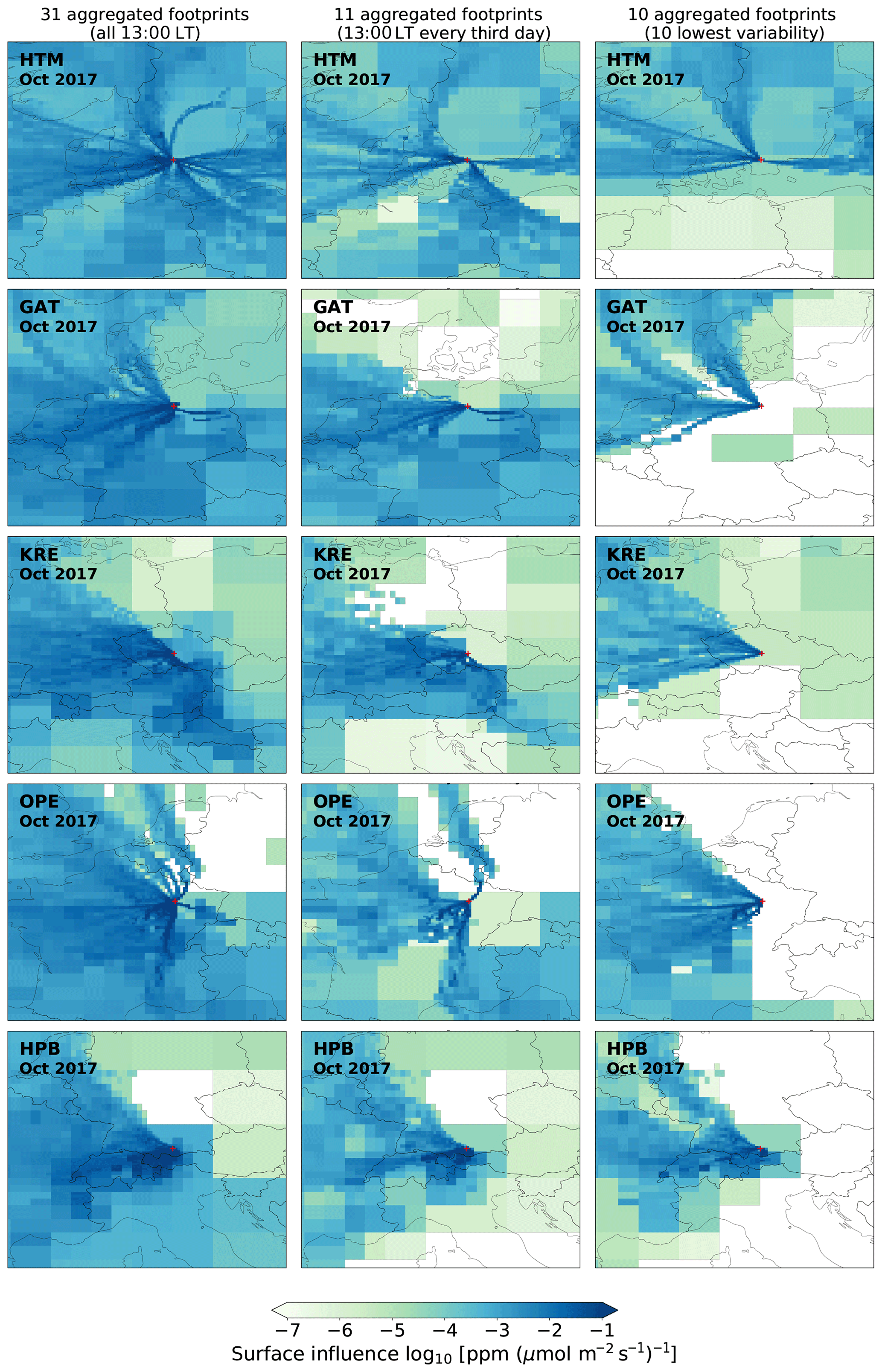
Figure 4 Aggregated footprints calculated for the five ICOS stations from top to bottom: Hyltemossa (HTM), Gartow (GAR), Křešín (KRE), Observatoire Pérenne de l'Environnement (OPE), and Hohenpeißenberg (HPB) for October 2017. The left column shows the footprints for all 31 d at 13:00 local time (LT), the middle column shows the same footprints, but sampled only every third day, and the right column shows those of the 10 d with the lowest variability. Note the logarithmic colour scale.

In addition to the footprint analysis, which gives a visual, qualitative idea of the effect of different flask sampling schemes, we evaluated the first 3 years of continuous CO₂ measurements from the five ICOS stations to quantify the effect of random sampling every 3 d versus only sampling low variability situations. Figure 5a–e show, in the upper panels, for each station, all available hourly atmospheric CO₂ data as grey dots, while the blue lines, each shifted by 1 d, connect the 13:00 LT data every 3 d. The red dots in the upper panels highlight the 10 lowest variability afternoon values in each month. As expected, all summer afternoon concentrations generally fall into the lower concentration range of the bulk of data. At all stations, the variability changes from a diurnal shape during the summer months to a more synoptic variability in the winter (for more details, also see Figs. 7 and 8). This synoptic variability is also represented in the afternoon sampling. In the middle panels of Fig. 5a–e we have plotted, as black dots, monthly means calculated from all afternoon hours between 11:00 and 15:00 LT and their standard deviations. The blue dots show the monthly mean values obtained from sampling every third day (the three different 3 d patterns are shown in individual shifted blue dots), while the red dots represent the monthly means calculated from the 10 samples with the lowest variability (the coloured dots were shifted by 1 d each for better visibility). It is obvious that regular sampling provides better representative monthly means, deviating in only a few cases from the all-afternoon means in CO₂ by more than 2 ppm (Fig. 5a–e, bottom panels). If samples were collected at low variability only, they would often underestimate monthly mean values, in some cases by more than 4 ppm (red lines in Fig. 5a–e, bottom panels). Although regular sampling every third day also introduces some variable deviations from the correct afternoon means, sampling only at low variability may introduce rather large biases – mainly towards lower CO₂ concentrations. Note that inversion models also select measured data for their inversion runs only for the time of the day, and not for low variability data, to estimate fluxes (Rödenbeck, 2005).

Figure 5 CO₂ concentration data measured at Hyltemossa (a), Gartow (b), Křešín (c), Observatoire Pérenne de l'Environnement (d), and Hohenpeißenberg (e). For each station the upper panel shows all hourly data as grey dots, while afternoon data (13:00 LT) from every third day are displayed as three blue lines shifted by 1 d each. Red dots highlight the 10 afternoon values with the lowest variability for each month. The middle panels show monthly means and standard deviations of all afternoon hours (11:00–15:00 LT) as black dots, respective means from afternoon data collected every third day are shown in blue, and means of the 10 afternoon values with the lowest variability are shown in red (for better visibility the coloured dots were shifted by 1 d each). The lower panels present the differences in the selected afternoon means from the respective mean calculated from all afternoon data.

We have investigated only potential sampling effects on CO₂ concentrations here; however, other tracer concentrations are also expected to be affected in a similar way. For the ICOS atmosphere network we, therefore, choose the simpler sampling scheme of one flask every third day. This sampling scheme is expected to serve aims 1 and 2, where those flasks with low within-hour variability (on average one flask per week; see Sect. 4.1) could be used for the quality control aim, while all flask samples would deliver as much representative data as possible for all additional trace components analysed in the FCL solely based on flasks.

4.3 Solutions and testing to meet aim 3: catching potentially high fossil fuel CO₂ events

The first ¹⁴C analyses on integrated CO₂ samples at ICOS stations showed rather low average fossil fuel CO₂ (ffCO₂) concentrations, therewith confirming that ICOS stations primarily monitor the terrestrial biospheric signals. Figure 6a–d (upper panels of the graphs for the individual stations) shows our first ¹⁴CO₂ results from the 2-week integrated CO₂ sampling at Hohenpeißenberg, Observatoire Pérenne de l'Environnement, Hyltemossa, and Křešín. Particularly during summer, the monthly mean regional fossil fuel CO₂ offsets, if compared to a background level calculated from the composite of 2-week integrated ¹⁴CO₂ measurements at Jungfraujoch in the Swiss Alps and Mace Head on the Irish coast, are often lower than a few parts per million (Fig. 6a–d, lower panels). Only during winter can regional ffCO₂ offsets reach 2-week mean concentrations of more than 5 ppm. These signals, although providing good mean ffCO₂ results for the average footprints of the stations, are often too small to provide a solid top-down constraint of regional fossil fuel CO₂ emission inventories and its changes when evaluated in regional model inversions (Levin and Rödenbeck, 2008; Wang et al., 2018). One of the aims of flask sampling in ICOS is, therefore, to explicitly sample air which has passed over fossil fuel CO₂ emission areas. Ideally we would like to obtain signals and analyse flasks for ¹⁴CO₂ only in cases when the expected fossil fuel CO₂ component is larger than 4–5 ppm. This would allow us to obtain an uncertainty of the estimated ffCO₂ component below 30 % (Levin et al., 2003; Turnbull et al., 2006). Furthermore, as sample preparation for ¹⁴C analysis is very laborious and the capacity of the CRL is limited to about 25 flask samples per station per year, one should know beforehand if a sample potentially contains a significant regional fossil fuel CO₂ component. This could either be found out with near real-time transport model simulations or directly using the in situ observations at the station.

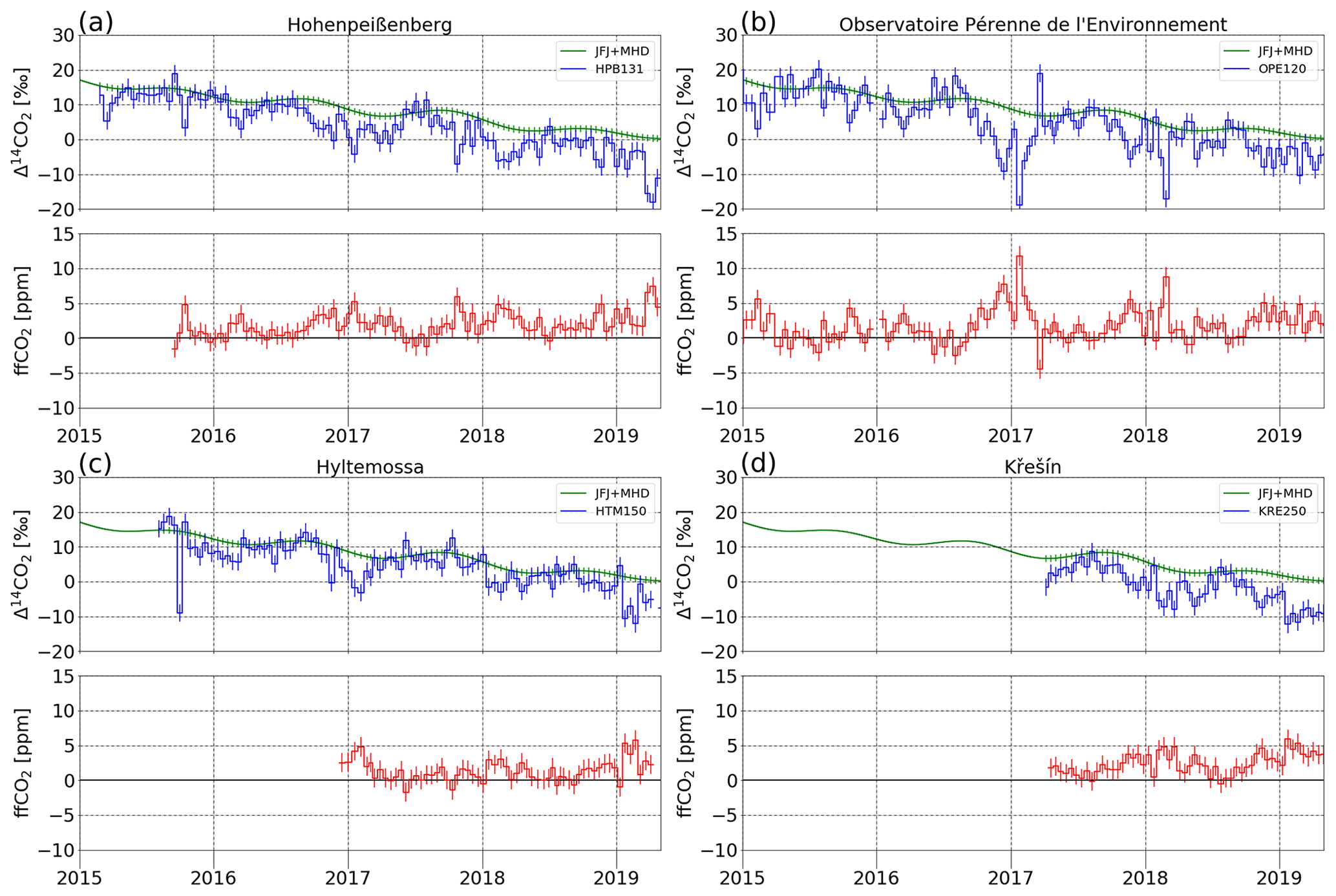
Figure 6 ¹⁴CO₂ observations and estimated fossil fuel CO₂ concentrations relative to European background at the ICOS stations (a–d) Hohenpeißenberg, Observatoire Pérenne de l'Environnement, Hyltemossa, and Křešín. The top panel for each station shows the Δ¹⁴CO₂ results in permil deviation from the National Bureau of Standards (NBS) oxalic acid standard (Stuiver and Polach, 1977) for the respective station (blue histogram) together with the European background, which is estimated as the fit curve to measured data from Jungfraujoch (JFJ) and Mace Head (MHD). The bottom panel for each station gives the regional fossil fuel CO₂ offset calculated from the ¹⁴CO₂ and CO₂ data, according to Levin et al. (2011). For Hohenpeißenberg and Hyltemossa, the ffCO₂ calculation starts later than the ¹⁴CO₂ data since no ICOS CO₂ data are available in the early periods for these stations.

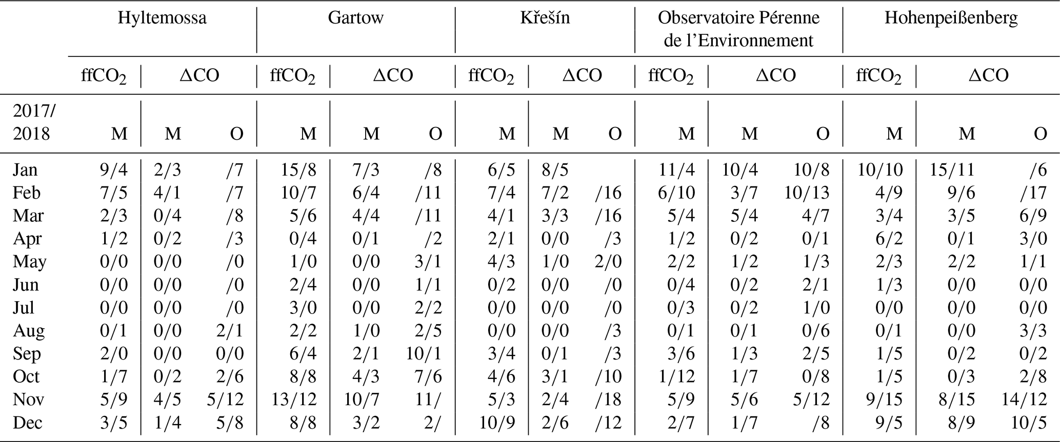
A good indicator of the potential regional fossil fuel CO₂ concentration at a station is the ambient CO concentration (Levin and Karstens, 2007), a trace gas that is monitored continuously at all ICOS Class 1 sites. It would then depend on the average CO:ffCO₂ ratio of fossil fuel emissions in the footprint of the stations to estimate, from the measured CO, the expected ffCO₂ concentration. Mean CO:ffCO₂ emission ratios can be very different in different countries; they mainly depend on the energy production processes and on domestic heating systems (Gamnitzer et al., 2006; Turnbull et al., 2006, 2011; Levin and Karstens, 2007; Vogel et al., 2010). In this respect, the share of biofuel use may also be relevant. In our study we first analysed our selected ICOS stations for regional fossil fuel CO₂ signals larger than 4 ppm and determined the frequencies of those events. Note that in order for the flask results to be used in transport model investigations, similar to all other flask samples, ¹⁴CO₂ flasks should also be collected during early afternoon when atmospheric mixing can be modelled with good confidence. During these situations, however, any ffCO₂ signals will be highly diluted. Similar to the approach in the previous section, we investigated the potential ffCO₂ levels for the five stations of Hyltemossa, Gartow, Křešín, Observatoire Pérenne de l'Environnement, and Hohenpeißenberg; this was first done theoretically with STILT model simulations transporting EDGAR version 4.3.2 emissions to the five measurement sites. As a second step, we evaluated the real continuous CO₂ and CO observations from 2017 and 2018 (see Table 1).

Table 1 Number of midday (13:00 LT) ffCO₂ events >4 ppm estimated by the Stochastic Time-Inverted Lagrangian Transport (STILT) model for 2017 and 2018 and potential fossil fuel CO₂ events in both years, based on modelled (M) and observed (O) ΔCO elevations of more than 0.04 ppm compared to background (entries are empty if fewer than 20 afternoon CO observations are available in the respective month).

4.3.1 Investigation of afternoon fossil fuel CO₂ events in 2017 at Gartow

Figure 7a–b show ambient STILT-simulated CO₂ and CO mole fractions at Gartow 341 m in July 2017 (13:00 LT values highlighted by coloured symbols), while Fig. 7c compares STILT-simulated total CO₂ (blue line) to observations (black line). The agreement between model and observations turned out to be reasonable, particularly during afternoon hours. In July 2017, deviations of the model simulations from observations are larger during night when the model seems to underestimate the measured concentration pile up. This model deficiency is the reason why we decided to collect the flask samples at midday or in the afternoon, making sure the data can be used in inversion estimates of fluxes. In Fig. 7d the simulated regional CO₂ components (ffCO₂ offset and biospheric CO₂ offset) originating from fluxes in the model domain covering the greater part of Europe are displayed, underlining the generally moderate fossil fuel CO₂ signal at Gartow in July. Indeed, summer situations with potentially high ffCO₂ concentrations are rare (one to five cases) at all ICOS stations and, at Gartow, only during 3 d; i.e. on 1, 7, and 27 July the modelled afternoon ffCO₂ was larger than 4 ppm (highlighted by red crosses in Fig. 7a). At the same time, the modelled CO offset was elevated but did not reach 0.04 ppm (Fig. 7b). CO offsets were estimated relative to the minimum modelled CO concentration of the last 3 d (grey line in Fig. 7b). In October 2017, the modelled (Fig. 8b) and measured CO (Fig. 8f) offsets do, however, rather frequently exceed 0.04 ppm. The generally good correlation between simulated ffCO₂ and CO offset can therefore be used as a criterion for ffCO₂ in collected flasks, and 0.04 ppm may be a good threshold for Gartow to predict a ffCO₂ signal of more than 4 ppm in sampled ambient air. This is supported by real observations displayed in Figs. 7f and 8f, where observed CO offsets >0.04 ppm (marked by magenta crosses) coincide with high total CO₂ and also with STILT-simulated ffCO₂ (see, for example, the synoptic event on 19–20 October 2017).

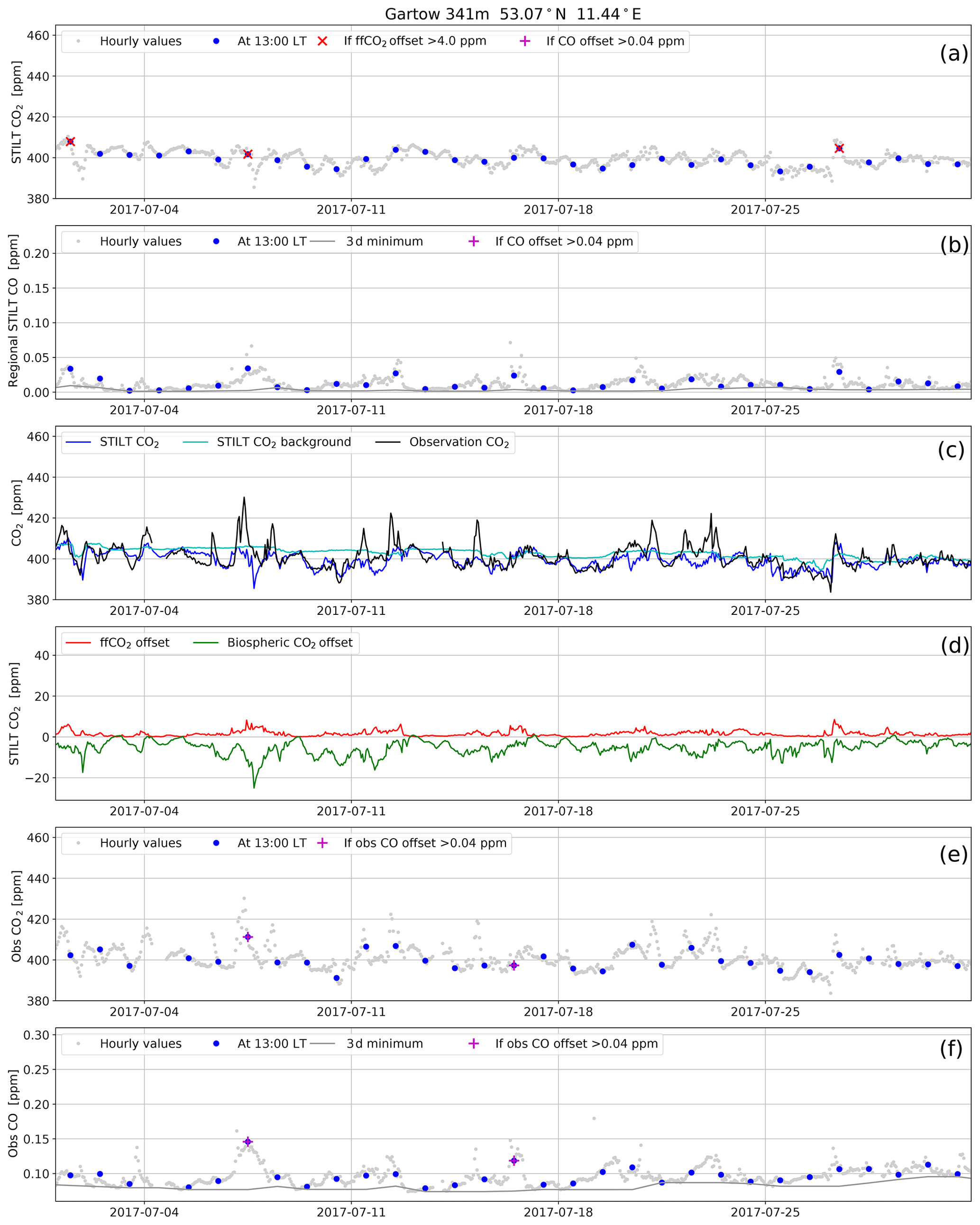
Figure 7 Variability of STILT-simulated (a–d) and measured (c, e, f) CO₂ and CO concentrations at Gartow at the 344 or 341 m level in July 2017. Afternoon values are highlighted with coloured symbols (blue dots) and situations with elevated ffCO₂, based on modelled or measured CO (CO offset >0.04 ppm), are marked with a magenta cross in the CO and also in the CO₂ records (clearer in Fig. 8 for October 2017 when such situations occur more often). CO offsets in STILT model simulations (b) and observations (f) were estimated relative to the minimum CO concentration of the last 3 d (grey lines).

Figure 8 Same as Fig. 7 but for October 2017.

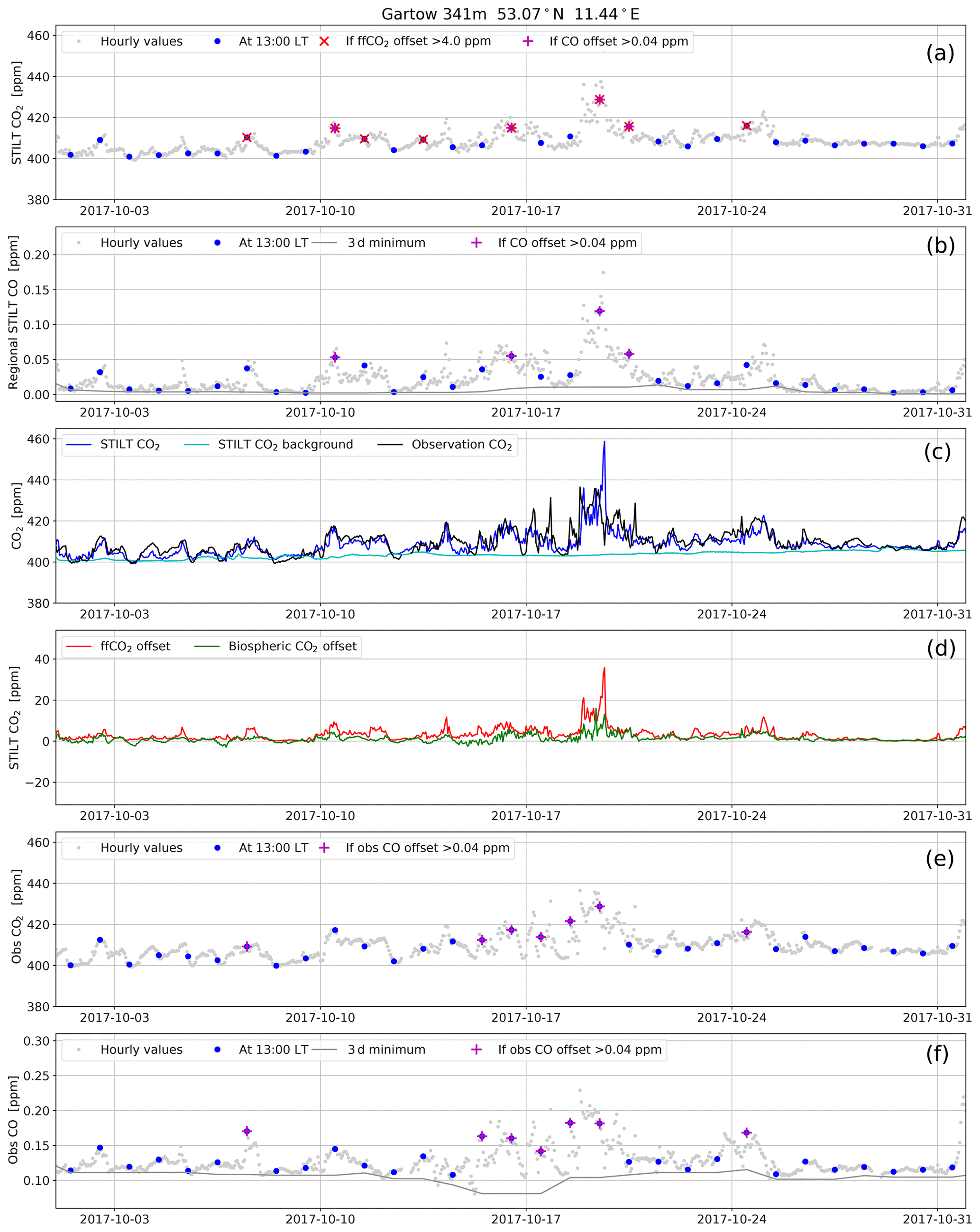
The aggregated footprints of the three afternoon situations with STILT-simulated ffCO₂ >4 ppm in July 2017 are displayed in Fig. 9a. They show southwesterly trajectories and a dominating surface influence from the highly populated German Ruhr area but also some influences from large emitters (e.g. power plants) in northwestern Germany and at the Netherlands' North Sea coast (see Fig. 9b). The main influence area with high ffCO₂ emissions in October 2017 (Fig. 9d) also shows Berlin as a significant emitter and some “hotspots” close to the German–Polish border in the southeast.

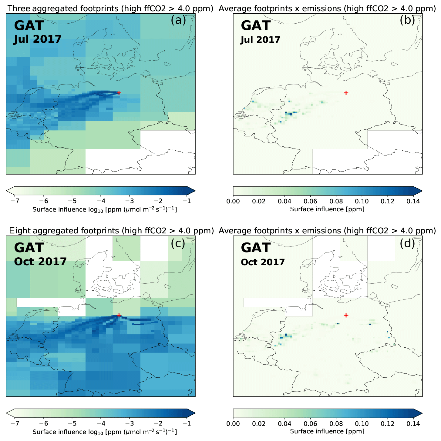
Figure 9 Aggregated footprints with elevated ffCO₂, and the corresponding surface influences for Gartow in July 2017 (a–b) and October 2017 (c–d), based on the EDGAR version 4.3.2 emission inventory. Note the logarithmic colour scale in the aggregated footprint maps.

4.3.2 Investigation of afternoon fossil fuel CO₂ events in 2017 and 2018 at Hyltemossa, Křešín, Observatoire Pérenne de l'Environnement, and Hohenpeißenberg

Overlapping measurements and STILT model runs are also available for the other four ICOS stations (Karstens, 2020). The general picture is similar here as in Gartow, but the number of elevated ffCO₂ events is often even smaller at these stations than at Gartow. For example, we find no ffCO₂ events at Hyltemossa, Gartow, Křešín, and Hohenpeißenberg and only three at Observatoire Pérenne de l'Environnement in July 2018 (Table 1). Simultaneously observed CO elevations relative to background are often only small in summer and do not reach the (preliminary) threshold of 0.04 ppm. Starting in October or November, ffCO₂ elevations become more frequent, coupled to the more synoptic variability of GHGs in the winter half-year (see Fig. 5a–e, upper panels). The number of modelled fossil fuel CO₂ events larger than 4 ppm for all months in 2017 and 2018, or based on observed CO offsets larger than 0.04 ppm using the same estimate for the CO background as for the model results displayed in Figs. 7b and 8b, are listed in Table 1. Only in the winter half-year can we potentially sample measurable fossil fuel CO₂ signals well. Lower ΔCO thresholds could be used for summer, which means accepting larger uncertainties of the ffCO₂ component. Although it would be most desirable to have a good ffCO₂ estimate in summer when the biospheric signal is large, our present measurement precision does not allow us to determine very small ffCO₂ contributions with good confidence. Therefore, we will currently have to restrict ¹⁴C analysis to flasks mainly collected in autumn, winter, and spring to constrain ffCO₂ emission inventories, with the additional advantage that the variability of biospheric signals is smaller during these seasons (see Fig. 8d).

To give some indication of the main ffCO₂ emission areas influencing the four stations, Fig. 10 shows aggregated footprints and the respective surface influence areas contributing to modelled ffCO₂ concentrations larger than 4 ppm in October 2017. At all four stations, and also at Gartow (Fig. 9), the areas potentially contributing significantly to the fossil fuel signals are located rather far away, and many of them are associated with large coal-fired power plants or other point sources. But a few big cities, such as Prague at Křešín, also occasionally contribute.

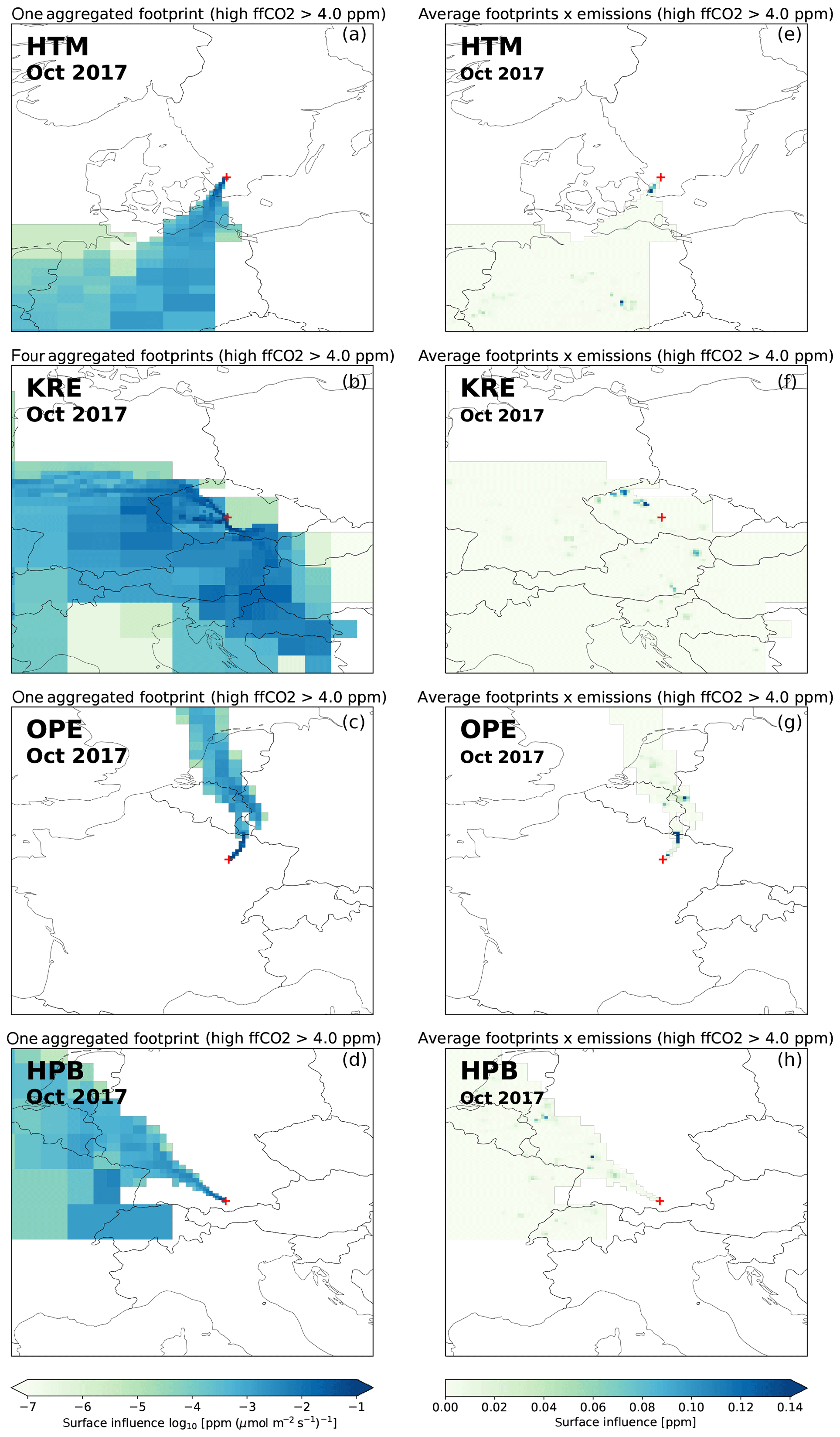
Figure 10 Aggregated footprints with elevated ffCO₂ and the corresponding surface influences for Hyltemossa (a, e), Křešín (b, f), Observatoire Pérenne de l'Environnement (c, g), and Hohenpeißenberg (d, h) in October 2017.

5 Implementation of the flask sampling scheme at ICOS stations

Sampling one flask every third day, independent of ambient CO₂ variability, can easily be implemented at ICOS stations, since sampling of all 24 flasks in the sampler can individually be programmed in advance. Assuming that flasks can be exchanged about once per month, during this time span 12 flasks would have been collected and could then be shipped in one box to the FCL for analysis. The remaining 12 flasks in the sampler would be reserved for ffCO₂ event sampling. In order to have a realistic chance to catch all possible events at a station, the sampler would be set to fill one of these flasks on each day in between the regular sampling every third day. As continuous trace gas measurement data are transferred from the station to the ATC every night, level 1 CO data are available on the morning after flask sampling the day before. These data will then be automatically evaluated at the ATC for potentially elevated CO to decide if the flask that had been collected on the day before potentially has an elevated ffCO₂ concentration and should be retained for ¹⁴CO₂ analysis. If yes, the flask sampler will receive a respective message from the ATC. If not, the flask can be resampled. Based on our analysis of modelled ffCO₂ for the years 2017 and 2018, the likelihood is small that more than 12 ffCO₂ events are sampled within 1 month. Also, some of the events may already have been sampled in one of the “regular”flasks sampled every third day. If this is the case, these flasks will be marked so that they are passed on to the CRL after analysis of all other components in the FCL. In the future, the flask sampling strategy, in particular, for ffCO₂ events might change once real-time GHG prediction systems or prognostic footprint products are available, which would allow more accurate targeting of certain emission areas. The first tests, using prognostic trajectories to automatically trigger ¹⁴CO₂ flask sampling, are made at the ICOS CRL pilot station and at selected ICOS Class 1 stations but are not yet mature enough to be implemented in the entire ICOS network. It is, however, also worth mentioning that sampling flasks during nighttime could largely increase the significance of ¹⁴C-based ffCO₂ estimates. Currently, we optimise our sampling strategy to meet the inability of transport models that are not digesting nighttime data. This situation is unfortunate and must urgently be improved in order to increase our ability to monitor, in a top-down way, long-term changes of the envisaged ffCO₂ emissions in Europe.

6 Conclusions

Although other flask sampling programmes from continental tall tower stations have similar aims, as presented here for ICOS, developing a dedicated sampling strategy to maximise the information from a minimum number of flasks is a new approach which, to our knowledge, has not yet been taken in any other sampling network. It may contribute to optimising efforts at the (remote) ICOS stations and the analytical capacities and capabilities of the ICOS Central Analytical Laboratories. Our strategy was designed to meet, on one hand, the requirements for quality control, making sure, by comparison of flask results with the parallel in situ measurements, that ICOS data are of highest precision and accuracy. Our first results showed that this strategy of independent quality control is working successfully. However, it requires fast turnaround of flasks in order to quickly detect errors in the in situ and also in the flask sampling systems. Besides ongoing QC, our sampling scheme will provide flask results that can be optimally used in current inverse modelling tasks to estimate continental fluxes, not only of core ICOS components, such as CO₂ and CH₄, but also of trace substances, which are not yet measured continuously. Trying to also monitor fossil fuel CO₂ emission hotspots at ICOS stations during well-mixed afternoon hours will be a particular challenge because the ffCO₂ influence at that time of the day is often very small, particularly in summer. There is thus an urgent need for transport model improvement so that nighttime data can also be used for the inversion of fluxes. Experience in the coming years will show if our current strategy is successful in meeting all the aims or if it needs further adaption.