Mid-level clouds are frequent above the southeast Atlantic stratocumulus clouds

Shortwave-absorbing aerosols seasonally overlay extensive low-level stratocumulus clouds over the southeast Atlantic. While much attention has focused on the interactions between the low-level clouds and the overlying aerosols, few studies have focused on the mid-level clouds that also occur over the region. The presence of mid-level clouds over the region complicates the space-based remote-sensing retrievals of cloud properties and the evaluation of cloud radiation budgets. Here we characterize the mid-level clouds over the southeast Atlantic using lidar- and radar-based satellite cloud retrievals and observations collected in September 2016 during the ORACLES (ObseRvations of Aerosols above CLouds and their intEractionS) field campaign. We find that mid-level clouds over the southeast Atlantic are relatively common, with the majority of the clouds occurring between altitudes of 5 and 7 km and at temperatures between 0 and −20 ^∘C. The mid-level clouds occur at the top of a moist mid-tropospheric smoke-aerosol layer, most frequently between August and October, and closer to the southern African coast than farther offshore. They occur more frequently during the night than during the day. Between July and October, approximately 64 % of the mid-level clouds had a geometric cloud thickness less than 1 km, corresponding to a cloud optical depth of less than 4. A lidar-based depolarization–backscatter relationship for September 2016 indicates that the mid-level clouds are liquid-only clouds with no evidence of the existence of ice. In addition, a polarimeter-derived cloud droplet size distribution indicates that approximately 85 % of the September 2016 mid-level clouds had an effective radius less than 7 µm, which could further discourage the ability of the clouds to glaciate. These clouds are mostly associated with synoptically modulated mid-tropospheric moisture outflow that can be linked to the detrainment from the continental-based clouds. Overall, the supercooled mid-level clouds reduce the radiative cooling rates of the underlying low-altitude cloud tops by approximately 10 K d⁻¹, thus influencing the regional cloud radiative budget.

1 Introduction

Clouds over the southeast Atlantic, as one of the world's major subtropical stratocumulus clouds (Klein and Hartmann, 1993), contribute importantly to the uncertainties in global climate change projections (Soden and Vecchi, 2011). Alone, these stratocumulus clouds cool the global climate system because they predominantly reflect the incoming shortwave radiation and exert a small effect on the outgoing longwave radiation (Wood, 2012). The stratocumulus clouds over the southeast Atlantic are different from others because they are accompanied by the presence of elevated smoke-aerosol layers in September and October when free tropospheric zonal winds emanating off of continental Africa are at a maximum (Adebiyi and Zuidema, 2016). This aerosol circulation pattern can strengthen the underlying low cloud deck through either meteorological or aerosol influences (Johnson et al., 2004; Wilcox, 2010; Adebiyi and Zuidema, 2018; Gordon et al., 2018; Deaconu et al., 2019). The interaction between the elevated smoke aerosols and stratocumulus clouds has received substantial attention in recent years from the research community because of its unique impact on the regional climate (Boucher et al., 2013). While the aerosol–stratocumulus–cloud interactions over southeast Atlantic complicate the estimation of the cloud radiative forcing, a recent study also highlights the presence of high moisture content that accompanies the smoke transport above the southeast Atlantic low-level clouds (Adebiyi et al., 2015). The occurrence of this high mid-tropospheric moisture points to the likelihood of mid-level clouds over the southeast Atlantic, which has not been highlighted in previous literature. The recent ORACLES (ObseRvations of Aerosols above CLouds and their intEractionS) field campaign (Redemann et al., 2020) observed such mid-level clouds (Fig. 1). Their location within and at the top of the smoke layer suggests potential interactions with the smoke aerosols (e.g., Lohmann and Feichter, 2005) that could further complicate the estimation of the cloud radiative forcing over the region. Whereas stratocumulus clouds tend to cool the regional climate, mid-level clouds with colder cloud tops and warming cloud radiative effects may likely offset the cooling effect associated with the stratocumulus clouds (Christensen et al., 2013; Bourgeois et al., 2016). Therefore, an accurate picture of the multilayer cloud system occurring in the presence of an elevated smoke layer is necessary to fully understand the complexity of the radiative interactions over the region.

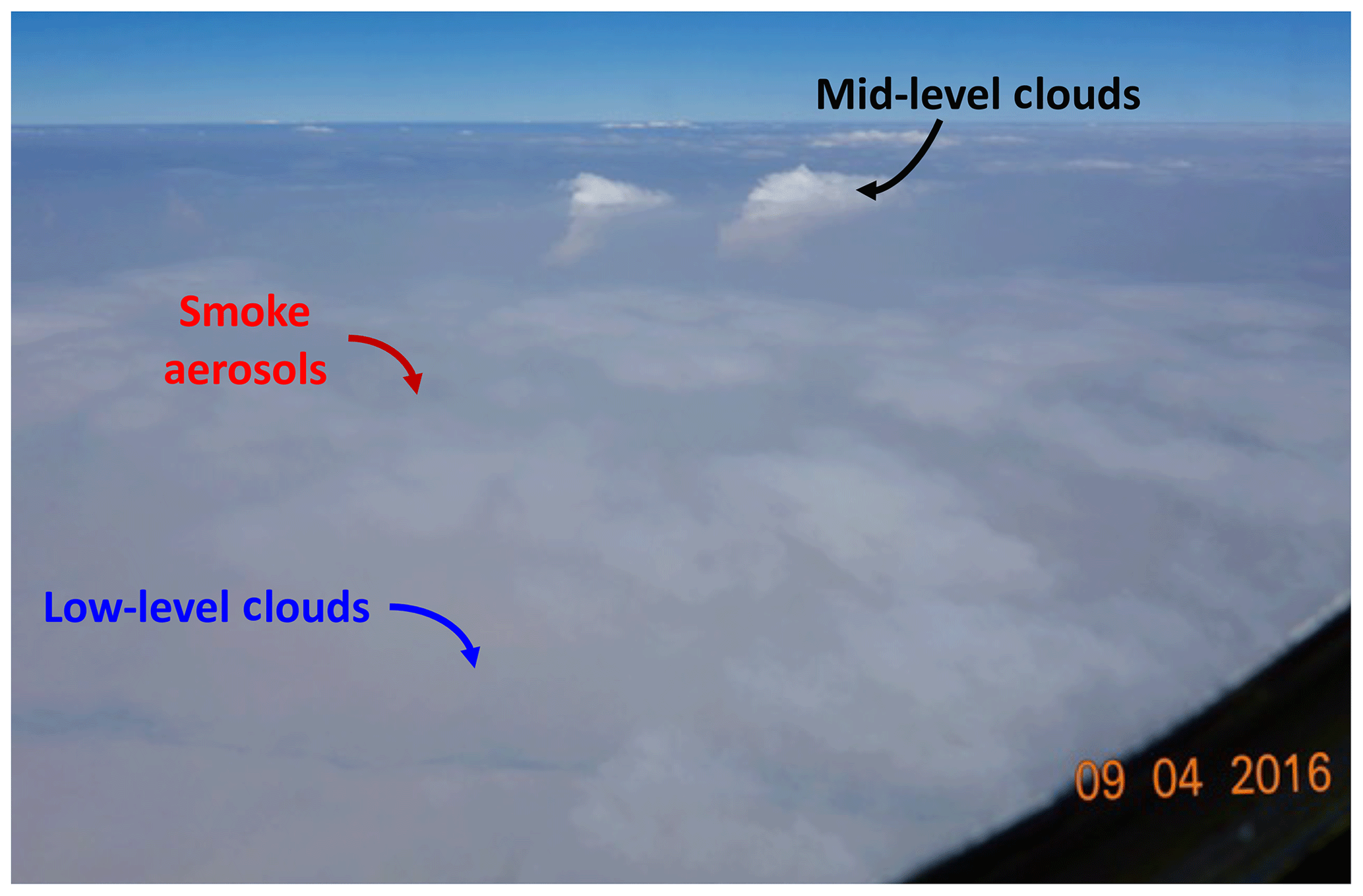
Figure 1 An Image taken during the NASA ORACLES Field campaign on 4 September 2016, showing mid-level clouds and smoke above the low-level clouds. Image taken by Paquita Zuidema.

Subtropical mid-level clouds have received less attention compared to those over equatorial or midlatitude regions (Fleishauer et al., 2002; Riley and Mapes, 2009; Stein et al., 2011; Riihimaki et al., 2012; Bourgeois et al., 2016, 2018). Globally, mid-level clouds cover about 25 % of the Earth's surface (Sassen and Wang, 2012) and account for about 30 % of all clouds (Zhang et al., 2010). With significant land–ocean contrast, the cross section of the mid-level cloud fraction generally increases from the tropical oceans to the midlatitude regions (Zhang et al., 2005, 2010; Bourgeois et al., 2016). In contrast to the midlatitude regions, there is a higher occurrence of nighttime mid-level clouds than daytime over the tropics (Zhang et al., 2010). Regardless of the clouds' location in the tropics or the midlatitudes, mid-level clouds mostly consist of supercooled liquid water, with most studies placing the temperature at the top of the clouds between 0 and −15 ^∘C with cloud thicknesses typically less than 2 km and cloud-top heights between 4 and 8 km (Riley and Mapes, 2009; Stein et al., 2011; Riihimaki et al., 2012; Bourgeois et al., 2018). With ice particles likely forming at a temperature less than −6 ^∘C (Hobbs and Rangno, 1985), the 0 to −15 ^∘C temperature range of the optically thin mid-level clouds suggests mixed-phase microphysics are possible (Zhang et al., 2010) with the potential impact on both the shortwave and longwave spectrum and cloud longevity.

Despite its significance, climate models have found it difficult to accurately simulate the distribution and properties of these mid-level clouds, and observational constraints by passive satellite sensors can be biased in multilayer cloud regions. Specifically, models consistently underestimate the mid-level clouds by simulating less than 40 % of the observed global distribution (Zhang et al., 2005). One reason for this underestimation is the misrepresentation of potential mixed-phase processes whereby liquid-water droplets and ice crystals may coexist and persist for long periods, thus presenting a unique challenge for global model parameterizations (e.g., Liu and Krueger, 1998). Another reason for the underestimation of mid-level clouds is because most models find it difficult to simulate multi-type multilayer cloud systems (Tselioudis and Kollias, 2007), thus overestimating high clouds due to their lack of detrainment of moisture by convection schemes at the mid-troposphere (Bodas-Salcedo et al., 2008). While cloud retrievals from space-based passive satellite sensors are often used as validation and an opportunity to improve these models, they also suffer in regions with multilayer cloud scenes (Holz et al., 2009). For passive sensors such as SEVIRI (Spinning Enhanced Visible and Infrared Imager) on board the Meteosat-10 satellite or MODIS (Moderate Resolution Imaging Spectroradiometer) on board the Terra satellite, multilayer cloud scenes often provide top-of-atmosphere radiances that are either too cold to be considered a lower-level cloud or too warm for the upper-level cloud retrievals (Davis et al., 2009), thus introducing uncertainties in the retrieved cloud properties.

In contrast, active remote-sensing measurements such as those from lidar and radar instruments can more easily identify the mid-level clouds and their properties in multilayer cloud scenes (Fig. 2a). These active sensors can be part of a ground-based station or mounted on an aircraft or a space-borne satellite. Over the southeast Atlantic, lidar measurements of clouds and aerosol vertical distributions were made from a high-altitude aircraft during the NASA ORACLES field campaign in September 2016 (Redemann et al., 2020). Passive shortwave spectral measurements made by the accompanying Research Scanning Polarimeter (RSP; Alexandrov et al., 2016) are furthermore novel in that properties of the mid-level cloud can be determined independently of those from the underlying low clouds. These measurements provided the first airborne observations of the mid-level cloud over the southeast Atlantic and confirmed the cloud's prevalence. However, these measurements only covered a short period and made it difficult to characterize the climatological state of the clouds over the region. Space-borne lidar and radar instruments on board the CALIPSO (Cloud-Aerosol Lidar and Infrared Pathfinder Satellite Observations; Winker et al., 2003) and CloudSat (Stephens et al., 2002) satellites respectively provide continuous spatial coverage and useful retrievals of clouds and aerosols over the southeast Atlantic. The combined information from CALIPSO and CloudSat provides a unique dataset that gives a reliable detection of the multilayer cloud system and its properties over the southeast Atlantic (Mace and Zhang, 2014). In this study, we use the aircraft measurements taken during the September 2016 ORACLES field campaign along with the CALIPSO only and CloudSat–CALIPSO merged datasets to document the characteristics and properties of the mid-level clouds above the southeast Atlantic stratocumulus clouds.

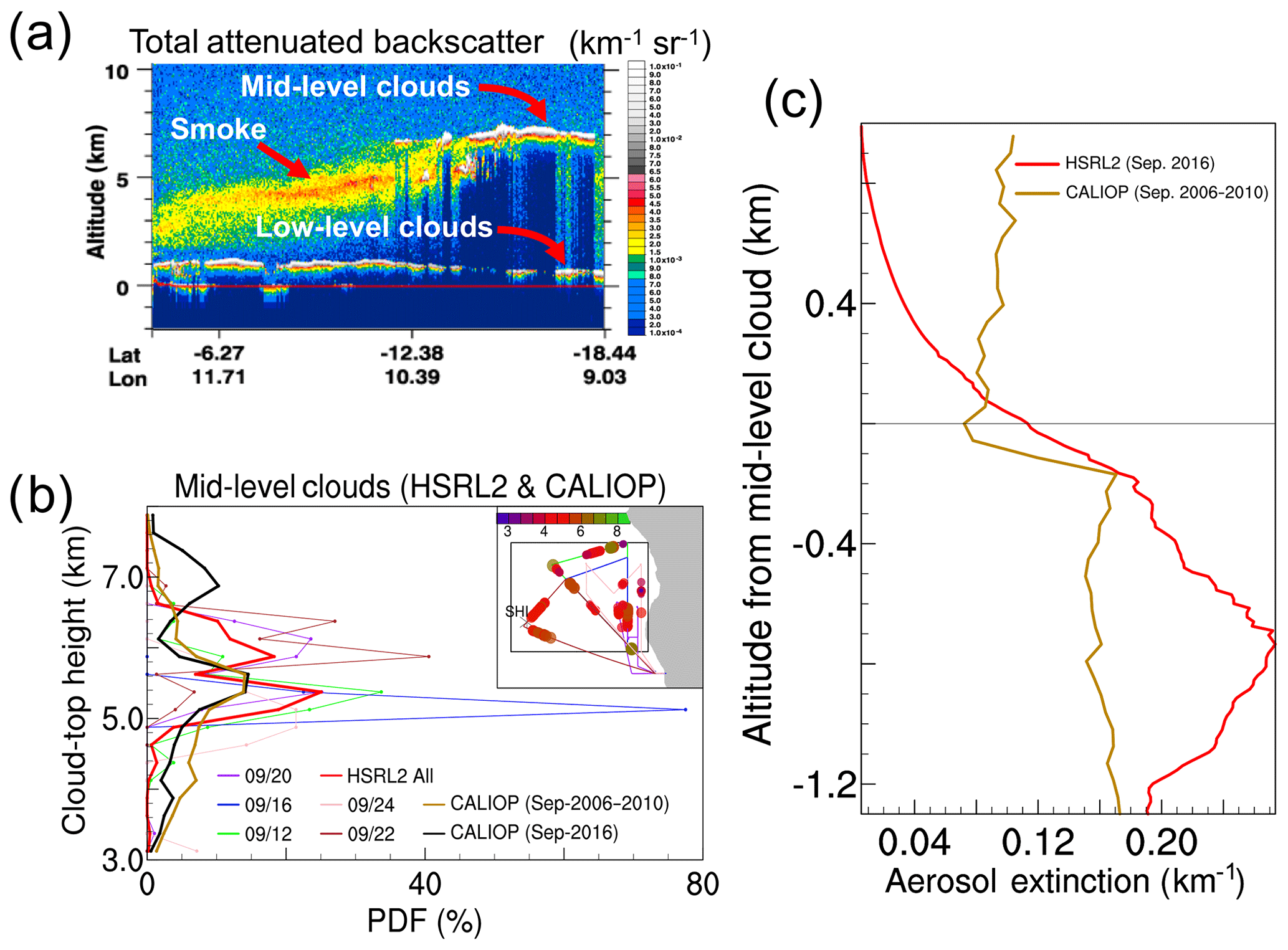
Figure 2 Mid-level clouds over the southeast Atlantic. (a) An example image from CALIPSO showing CALIOP 532 nm total attenuated backscatter (km⁻¹ sr⁻¹) with identifiable mid-level clouds, smoke, and low-level clouds on 22 September 2016 between ∼ 00:54 and ∼ 00:57 UTC over the southeast Atlantic. (b) The probability distribution of mid-level cloud-top heights (km) measured by the HSRL-2 on board the ER-2 high-altitude aircraft during ORACLES in September 2016. The combined distribution from HSRL-2 is shown by the thick red line, while the CALIOP distribution for all available CALIPSO overpasses for September 2016 and September 2006–2010 are shown by the thick black and brown lines respectively. The inset in (b) shows the spatial locations and heights (km) of the HSRL-2 mid-level cloud measurements, as well as the region for the CALIOP distribution (5–20 ^∘ S and 10^∘ W–12^∘ E). (c) The 532 nm aerosol extinction coefficients (km⁻¹) averaged horizontally for a 0.2^∘ grid box above and below the mid-level cloud top obtained from HSRL-2 (red line; September 2016) and from CALIOP (brown line; September 2006–2010).

2 Data and methods

We define the mid-level clouds as clouds between 3 and 8 km which are above the low-level clouds over the southeast Atlantic. These altitude levels correspond to the standard pressure of approximately 700 to 350 hPa. Our definition of the mid-level cloud is consistent with previous studies (e.g., Riihimaki et al., 2012; Bourgeois et al., 2016, 2018), and we use it here also because the inversion-capped low-level clouds are generally topped below 3 km over the southeast Atlantic (e.g., Painemal et al., 2014; Adebiyi et al., 2015). We focus our analysis primarily on the region between 5 and 20^∘ S and 10^∘ W and 10^∘ E, which is approximately the region that was covered by the 2016 ORACLES field campaign and is also the region dominated by climatological low-level clouds between July and October over the southeast Atlantic (Zuidema et al., 2016). Since this delimited area is part of the larger southeast Atlantic region, our analysis thus considers the entire southeast Atlantic region to provide a broader context for the occurrence of mid-level clouds beyond the area covered by ORACLES.

We primarily use the cloud information measured by the second generation airborne High Spectral Resolution Lidar (HSRL-2) on board the NASA ER-2 aircraft during the September 2016 ORACLES field campaign (hereafter called ORACLES-2016). ORACLES-2016 was conducted out of Walvis Bay in Namibia. Unlike other subsequent ORACLES deployments in August 2017 and October 2018 that operated out of São Tomé and Príncipe, only ORACLES-2016 deployed the ER-2 aircraft, which is capable of reaching above 20 km in altitude (Redemann et al., 2020). HSRL-2 measures backscatter, extinction, and the depolarization ratio of atmospheric constituents at 355 and 532 nm and also the backscattering and the depolarization ratio at 1064 nm (Burton et al., 2018). The vertically resolved multiwavelength and depolarization measurements of mid-level clouds are invaluable for accurately distinguishing the altitude and phase of the mid-level clouds, which provides a unique view of the multilayer cloud and aerosol system over the southeast Atlantic. Details of the instrument, calibrations, and algorithms can be found in Burton et al. (2015, 2018) and the references therein. Of the 12 ER-2 flight days conducted during ORACLES-2016, each between 7 and 9 h in duration, HSRL-2 was active for 7 d. We use the HSRL-2 version R7 data with a vertical resolution of 15 m and a horizontal resolution of 10 s or approximately 1.8 km. Therein, we primarily use the HSRL-2 cloud-top heights, aerosol extinction, particulate backscatter, and particulate depolarization ratio information at 532 nm. We also use the temperature information from the Modern-Era Retrospective analysis for Research and Applications Version 2 (MERRA-2; Gelaro et al., 2017) reanalysis that is collocated to the HSRL-2 measurements.

A secondary source of information on mid-level clouds comes from the Research Scanning Polarimeter (RSP) which was also on board the NASA ER-2 during ORACLES-2016. RSP was active on all 12 ER-2 flight days, and we use RSP V003 data with a horizontal resolution of approximately 200 m for cloud screening and 1 km for cloud retrievals. The RSP measures the Stokes parameters I, Q, and U simultaneously at nine wavelengths while scanning through ±60^∘ along the aircraft ground track providing multi-angle views of each ground/cloud pixel (Cairns et al., 1999). The spectral bands at 865 and 1880 nm are of particular relevance for detecting and characterizing the droplet size distributions of mid- and low-level clouds. Measurements in the 1880 nm spectral band are essentially insensitive to the low-level marine boundary layer (MBL) clouds because of strong water vapor absorption in this spectral band (Gao et al., 2004) and the fact that there is a moist layer above the MBL. For example, with the sun overhead and a viewing angle of 60^∘, the two-pass transmission at 1880 nm from the sun to the MBL cloud and back to the RSP is ∼0.001 for 1 precipitable centimeter of column water vapor. This allows for the robust detection of mid-level clouds using the 1880 nm band even when there are underlying MBL clouds. Observations of the polarized cloud bow at 865 and 1880 nm can then be used to determine the parameters (effective radius and variance; Hansen and Travis, 1974) of a cloud droplet size distribution (DSD), and at 865 nm a nonparametric DSD can also be retrieved through the use of a rainbow Fourier transform (RFT; Alexandrov et al., 2012). When there are multiple cloud layers, such as when mid-level clouds overlie MBL clouds, the RFT can be used to distinguish the effective radius and variance of multiple layers through a modal decomposition (Alexandrov et al., 2016). In this work, a mid-level-cloud effective radius and variance are assigned when only a mid-level cloud is present and also when there is an underlying MBL cloud. In both cases, the modal decomposition of the RFT is used, with the mode assigned to the mid-level cloud having an effective radius that is closest to that determined from a parametric DSD retrieval using 1880 nm cloud bow observations. This approach is taken because the cloud bow observed at 1880 nm for a given size distribution is broader and weaker than that at 865 nm, which reduces the accuracy of the parametric DSD estimate. In addition, the mid-level cloud bow signal at 1880 nm is often quite weak because the clouds are optically thin and/or embedded in the moist layer above the MBL. Since cloud modes are generally separated in effective radius by 5–10 µm, the use of the effective radius derived at 1880 nm only provides a categorical assignment of mode that mitigates against these issues. Further ancillary datasets used to characterize the mid-level cloud properties are in situ measurements gathered by the P-3 plane within and below the mid-level clouds on 4 September (depicted in Fig. 1) and 24 September 2016 (see the Supplement). A regional climatology of the mid-level cloud properties over the southeast Atlantic was developed from the cloud retrievals from the CloudSat and CALIPSO products (Stephens et al., 2002; Winker et al., 2003). Both CloudSat and CALIPSO are part of the A-Train constellation with footprints overlapping more than 90 % of the time (Stephens et al., 2008). While CloudSat carries a 94 GHz cloud profiling radar (CPR), CALIPSO carries the Cloud-Aerosol Lidar with Orthogonal Polarization (CALIOP). Although the instruments are built differently, both are able to observe the atmospheric vertical distributions, with the CALIOP lidar being more sensitive to the aerosols and optically thin clouds than the CPR radar (Mace and Zhang, 2014). In contrast, the CPR radar is suitable for an optically thick cloud layer, and it is able to determine the phase and other microphysical properties of the cloud better than the CALIOP lidar (Sassen and Wang, 2008). The combined product thus provides unique data useful for understanding the macro- and micro-physical characteristics of the mid-level clouds above the optically thick stratocumulus clouds. In this study, we use the CALIOP retrievals to determine the height level of the mid-level clouds, including the cloud-top heights, and we use the CloudSat–CALIPSO merged dataset to analyze the essential cloud properties. We obtain the mid-level cloud-top heights and aerosol extinction at 532 nm wavelength from version 3 of level 2 CALIOP Layer_Top_Altitude and Extinction_Coefficient_532 products. Although there were some improvements in the version 4 cloud–aerosol discrimination algorithm, most of them were specifically focused on aerosol lofted into the upper atmosphere or the lower stratosphere (Liu et al., 2019). As a result, more than 95 % of all aerosol and cloud layers detected within the troposphere remain largely unchanged between versions 3 and 4 (Liu et al., 2019). Using the Layer_Top_Altitude product, we determine the cloud-top height (km) as the mid-level cloud layer top and the frequency of occurrence of mid-level cloud as the number of CALIOP profiles with observed mid-level clouds divided by the total number of observations over the regions. Furthermore, we also rely on three products from the merged CloudSat–CALIPSO datasets: 2B-GEOPROF-LIDAR which provides the fraction of hydrometeor in each layer (Mace and Zhang, 2014), 2B-TAU which provides the cloud optical depth, and 2B-FLXHR-LIDAR which provides estimates of broadband fluxes and radiative heating rates in the atmospheric column (L'Ecuyer et al., 2008; Henderson et al., 2013). Specifically, the LayerTop and LayerBase variables from the 2B-GEOPROF-LIDAR product determine the heights, frequency of occurrence, and the geometric thickness (top minus base) of the mid-level cloud layers defined between 3 and 8 km. The layer_optical_depth_2B_TAU variable from the 2B-TAU product indicates the optical depth for the identified mid-level cloud layer, and QR_2B_FLXHR_LIDAR from the 2B-FLXHR-LIDAR product indicates the heating rates at the top of the low-level clouds. For the latter, the underlying low-level clouds are defined for cloud layers identified below ∼3 km. In addition, the low-level cloud-top heating rates are assessed for cases when there are collocated overlying mid-level clouds and when there are none. While the level 2 CALIOP products are reported at a horizontal resolution of 5 km and vertical resolution between 60 and 360 m (Hunt et al., 2009), the combined products have a horizontal resolution of approximately 1.3 km by 1.7 km, and the effective vertical resolution at nadir is 240 m (Stephens et al., 2008). Although CALIOP retrievals extend to the present day, we analyze the mid-level cloud properties only between 2006 and 2010, where both sensors measure the atmospheric volume within 15 s of each other, and high-quality products are available for both the CALIOP and CloudSat–CALIPSO merged products. We ignore data after 2010 because of a battery anomaly that caused the CloudSat satellite to stop collecting data and eventually lose formation with the A-Train constellation in 2011 (Nayak et al., 2012). While CloudSat rejoined A-Train in June 2012, it was positioned in a different satellite constellation such that its observing time is 100 s different from CALIOP. Furthermore, CloudSat only acquired measurements during the daytime in the post-anomaly period, resulting in about a 50 % reduction in the sampling size compared to the pre-anomaly period (Mace and Zhang, 2014).

In addition to the cloud information from ORACLES and CloudSat–CALIPSO merged datasets, other datasets helped characterize the variability of the mid-level clouds and their large-scale environment. We obtain the temperature, moisture, and wind information over the southeast Atlantic region from the European Centre for Medium-Range Weather Forecasts (ECMWF) ERA-Interim reanalysis (Dee et al., 2011) in addition to ECMWF auxiliary data that have been interpolated to CloudSat and CALISPO bins (Partain, 2007). We also obtain additional cloud and aerosol information of daily averaged retrievals from the Moderate Resolution Imaging Spectroradiometer (MODIS) and the Meteosat-10 Second Generation (MET10) satellites. Specifically, we obtained the MODIS-Terra low-level cloud fraction and aerosol optical depth retrievals (King et al., 2013), as well as cloud-top heights and brightness temperature, from the Spinning Enhanced Visible and Infrared Imager (SEVIRI) instrument on board the MET10 satellite (Schmetz et al., 2002). In particular, we use the cloud information from SEVIRI to assess the diurnal and spatial variability of the mid-level clouds. Although a passive instrument such as SEVIRI has difficulty accurately capturing the cloud-top heights when a mid-level cloud is above an optically thick low-level cloud (Fig. 3; see also Fig. S1), they are useful because of their broad swaths and high temporal resolution. SEVIRI on board the geostationary MET10 satellite sits at 35 786 km altitude centered at approximately 9.5^∘ E longitude with cloud observations at a temporal resolution of 15 min and a 3 km spatial resolution at the sub-satellite point. We use both the brightness temperature directly retrieved at the 10.8 µm infrared channel and the cloud-top heights retrieved using the NASA Langley cloud product algorithm. While details can be found in Minnis et al. (1995), this algorithm combines techniques that use the information which spans from visible (0.65 µm) to infrared (10.8 µm) channels to obtain improved retrieval accuracies (Palikonda et al., 2006).

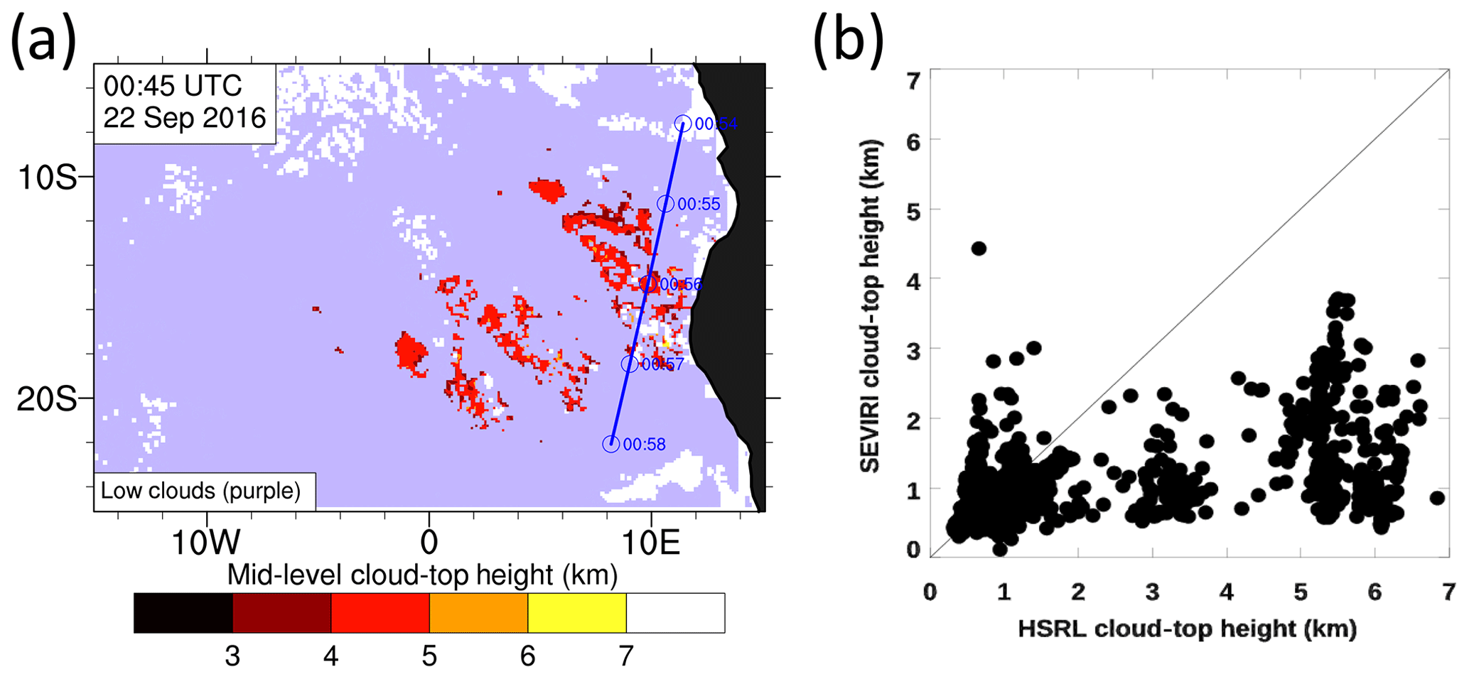
Figure 3 Comparison between mid-level clouds observed by SEVIRI and lidar-based instruments. (a) Image from the SEVIRI instrument corresponding to the CALIPSO image in Fig. 2a. This was taken at 00:45 UTC on 22 September 2016, and it shows the mid-level cloud-top heights (km; red-yellow shade) and the low-level clouds (purple; defined by cloud-top heights less than 3 km) over the southeast Atlantic. The blue line is the CALIPSO crossover track for the image in Fig. 2a, although it occurs 9 min after the satellite image. (b) Comparison between SEVIRI and HSRL-2 cloud-top height collocated within ±15 min of each other during ORACLES-2016.

3 Results

An example of the vertical profile of the total attenuated backscatter from CALIPSO shows that the southeast Atlantic features not only the presence of the elevated smoke and the low-level clouds but also the mid-level clouds (Fig. 2a). For this example, these mid-level clouds are between 12 and 18^∘ S, and they significantly attenuate the lidar signal directly below them (see more CALIPSO images in Supplement Fig. S2). We document here the occurrences (Sect. 3.1), the properties (Sect. 3.2), the associated large-scale meteorology (Sect. 3.3), the radiative impacts on the low-level clouds (Sect. 3.4), and the diurnal variability (Sect. 3.5) of the mid-level clouds to provide a full picture of the complicated cloud–aerosol system over the southeast Atlantic.

3.1 Occurrence of mid-level clouds over the southeast Atlantic

During the ORACLES-2016 campaign, mid-level clouds were observed in 5 out of 7 d that the HSRL-2 was active over the southeast Atlantic (Fig. 2b). Although the observation of mid-level clouds occurs over most parts of the campaign region, their cloud-top heights are generally below 7 km (see inset in Fig. 2b). To better understand what the preferred altitude levels are for the mid-level clouds, we estimate the probability distributions of the HSRL-2 cloud-top heights and compare with those from CALIOP during September over the campaign region (Fig. 2b). We found that the majority of the HSRL-2 mid-level cloud-top heights occur between 5 and 7 km with the median value at approximately 5.4 km and the probability distribution collectively reaching up to about 25 %. Although CALIPSO overpasses in September 2016 do not directly correspond to the locations and time of the HSRL-2-inferred mid-level clouds, they similarly show that the clouds appear to have a preferred altitude between the 5 and 7 km range. In fact, the CALIOP distribution of the mid-level cloud climatology for all of September between 2006 and 2010 agrees remarkably well with the distribution that uses only the values in September 2016 or for the few days of the HSRL-2 observations. Overall, about 93 % of the mid-level cloud-top heights measured during ORACLES-2016 are above 5 km compared to ∼77 % and ∼61 % from the CALIOP-derived mid-level clouds respectively for September 2016 and September 2006–2010.

The mid-level clouds typically occur in the presence of smoke aerosols over the southeast Atlantic. As the CALIOP attenuated backscatter example shown in Fig. 2a, the smoke aerosols are typically found immediately below the mid-level clouds, although there are cases where the clouds form inside the elevated smoke-aerosol layer (see also Figs. 1 and S2). Indeed, further analysis of HSRL-2 and CALIOP extinction profiles in September shows that the averaged aerosol extinction coefficients over a 1 km layer immediately below the mid-level clouds are about 0.21 and 0.14 km⁻¹ respectively (Fig. 2c). While humidity can increase the aerosol scattering (e.g., Magi and Hobbs, 2003), these values are markedly higher than the 0.03 and 0.10 km⁻¹ for the corresponding 1 km layer above the clouds for HSRL-2 and CALIOP respectively. The HSRL-2 profiles in September 2016 indicate a cleaner layer above the mid-level clouds, with the aerosol extinction coefficient decreasing to zero faster than those observed from CALIOP (Fig. 2c). As the CALIOP image in Fig. 2a also suggests, the mid-level clouds and the smoke layer also occur over a region that is usually covered by underlying warm liquid clouds during September (e.g., Adebiyi et al., 2015).

While the ORACLES-2016 and CALIPSO observations shown in Fig. 2 are for September, the mid-level clouds over the southeast Atlantic are also present in other months. Fig. 4a shows that the mid-level clouds are more prevalent between August and October compared to other months. The frequency of occurrence – estimated hereafter as the number of profiles of the mid-level clouds divided by the total number of observations – shows a minimum of about 2 % in June and a maximum of about 15 % in September when averaged over the ORACLES-2016 campaign region (5–20^∘ S and 10^∘ W–10^∘ E; inset in Fig. 2b). Furthermore, the seasonal cycle of the mid-level clouds overlaps with that of the smoke-aerosol loading, further highlighting the co-occurrence of the smoke aerosols with the mid-level clouds. Of particular interest is the time period between July and October because that is when the smoke-aerosol loading and the underlying low-level cloud fraction simultaneously reach their climatological maximum (Fig. 4a). Therefore, we examine the spatial distribution of the mid-level cloud regional climatology between July and October (Fig. 4b and c). We find that the mid-level clouds are common near the coast with a frequency of occurrence of up to 30 % that gradually decreases westward (Fig. 4b). For those above the climatologically high low-level cloud region north of 20^∘ S (black contour in Fig. 4b), the mean mid-level cloud-top heights are overwhelmingly between 5 and 6 km. In contrast to north of ∼20^∘ S, the mid-level clouds south of 20^∘ S occur less frequently at about 10 %–15 % and are higher with a mean cloud-top height increase of about 1 km (Fig. 4b and c). This contrast between the mid-level clouds north and south of ∼20^∘ S highlights the complexity and variability of the cloud systems over the southeast Atlantic. Unlike north of 20^∘ S, which is dominated by separated low-level and mid-level clouds, the cloud system south of 20^∘ S often occurs as a unified deep-convective cloud system extending from the low-level to upper-level atmosphere as part of the eastward-traveling midlatitude disturbances (Adebiyi and Zuidema, 2018). As a result, the isolated mid-level cloud is not as common south of 20^∘ S as it is north of 20^∘ S.

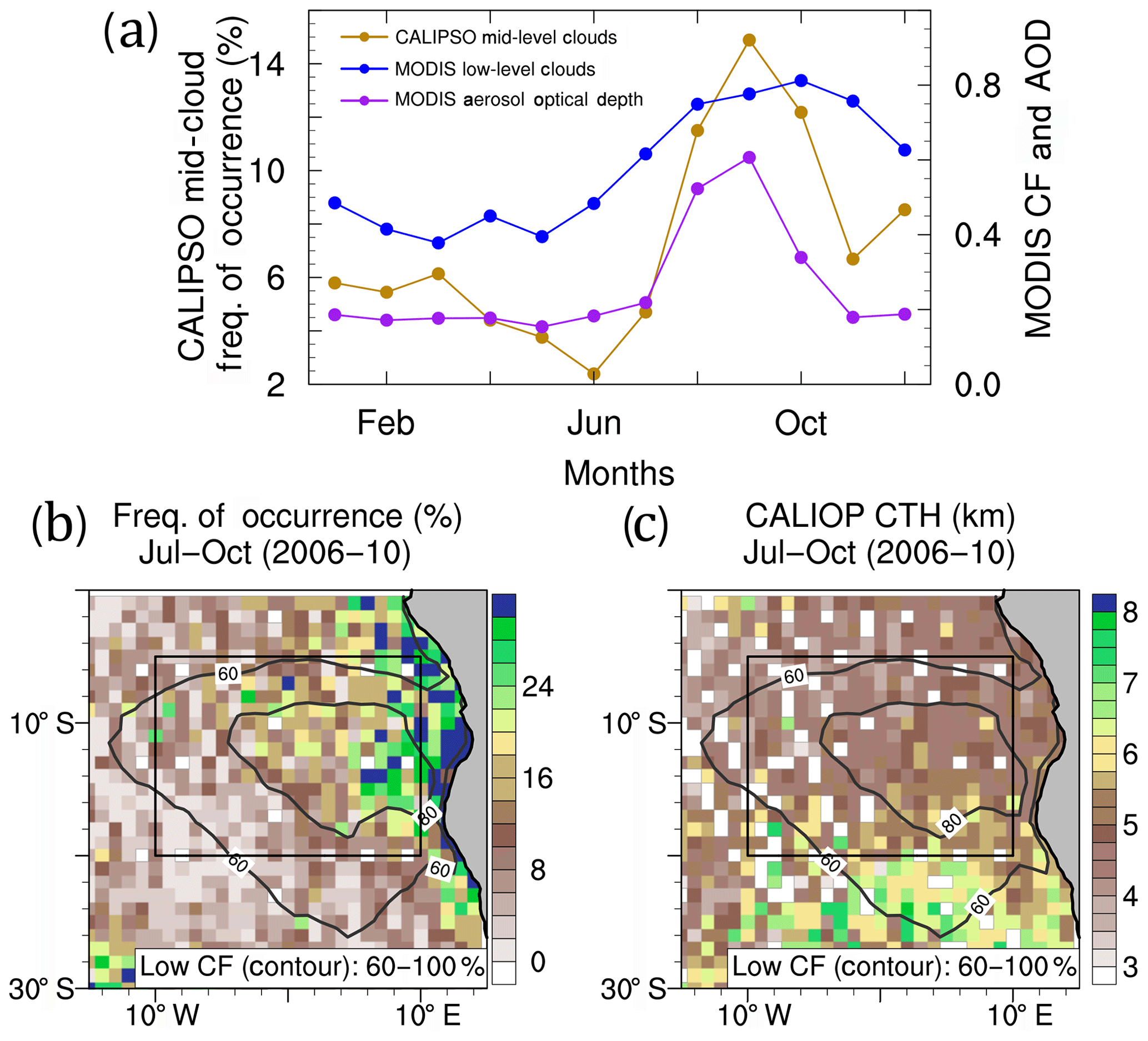
Figure 4 (a) Monthly averages (2006–2010) of the CALIPSO mid-level cloud frequency of occurrence (%; brown line) and MODIS low-level cloud fraction and aerosol optical depth (CF and AOD; right axis), all averaged over the ORACLES-2016 campaign region (defined here as 5^∘–20^∘ S and 10^∘ W–10^∘ E; black boxes in b and c). (b) The spatial distribution of the July–October average for the CALIPSO mid-level cloud frequency of occurrence (%) and (c) the corresponding cloud-top heights (km). The black contours in both (b) and (c) are the MODIS liquid-water low-level cloud fraction (%) for the same period. The CALIPSO mid-level clouds are identified as the cloud-top layer between 3 and 8 km, while the MODIS low-level clouds are averages of grid boxes with cloud-top temperatures greater than 273 K.

3.2 Properties of the mid-level clouds

We focus on the region north of 20^∘ S and examine the properties of the mid-level clouds using the observations during the ORACLES-2016 campaign and the merged CloudSat–CALIPSO datasets. We analyze the probability and the cumulative distributions (Fig. 5a–c) of the mid-level cloud optical depth, its geometric thickness (km), and cloud temperature (^∘C). Similar to the CALIPSO analysis, the majority of the mid-level cloud-top heights for the merged CloudSat–CALIPSO datasets between July and October is also between 5 and 7 km (compare Figs. 2 and S3a). Furthermore, the cloud geometric thickness and the cloud optical depth are predominantly less than 1 km and 4 respectively (Fig. 5a and b). Specifically, approximately 64 % of the mid-level clouds have a cloud thickness that is less than 1 km (85 % for a thickness of less than 1.5 km), and about 60 % have a cloud optical depth that is less than 4 (72 % for an optical depth of 6). For comparison, the same thickness in stratocumulus clouds could have a cloud optical depth greater than 20 (e.g., Szczodrak et al., 2001; Haywood et al., 2004). These results thus suggest that the mid-level clouds over the southeast Atlantic are geometrically and optically thin clouds.

In addition to the southeast Atlantic mid-level clouds being optically thin, these mid-level clouds also have distributions that span warm to cold temperatures. Figure 5c and d show the temperature distribution of the mid-level clouds respectively obtained for the CloudSat–CALIPSO merged dataset between July and October (2006–2010) and for the mid-level clouds observed during ORACLES-2016. For both cases, the temperature distributions generally extend from −20 ^∘C to about 4 ^∘C with the majority of the mid-level clouds colder than 0 ^∘C. Specifically, about 98 % and 87 % of the mid-level clouds obtained from the field campaign and merged CloudSat–CALIPSO datasets respectively have cloud-top temperatures below 0 ^∘C (gray lines in Fig. 5c and d). In addition, the majority of the cold mid-level clouds are observed above 5 km, which is evident in the CloudSat–CALIPSO dataset (Fig. 5c) and in the HSRL-2 datasets with observed mid-level clouds generally above 5 km (Figs. 5d and 2b). Furthermore, the mid-level clouds also show double peaks in the probability distribution for both CloudSat–CALIPSO and HSRL-2 datasets: one around −4 ^∘C and the other around −9 ^∘C. For the CloudSat–CALIPSO dataset, the warmer peak ($\sim -\mathrm{4}$ ^∘C) corresponds to mid-level cloud-top heights less than 6 km, while the colder peak ($\sim -\mathrm{9}$ ^∘) corresponds to cloud-top heights higher than 6 km (Fig. 5c). This double peak in temperature distribution over the southeast Atlantic is similar to those documented for tropical and midlatitude mid-level clouds (e.g., Riihimaki et al., 2012; Riley and Mapes, 2009). However, one notable difference is that our second temperature peak ($\sim -\mathrm{9}$ ^∘C) is markedly warmer than previously reported for other regions (which is typically between −12.5 and 15 ^∘C). Potential reasons for this difference are explored in Sect. 3.3.

Figure 5 The probability (PDF; solid black lines) and cumulative (CPDF; dashed gray lines) distributions of mid-level cloud properties. These distributions are obtained for mid-level (a) cloud thickness (km), (b) cloud optical depth, and (c) cloud temperature (^∘C) from the CloudSat–CALIPSO merged dataset between 3 and 8 km altitude in July and October (2006–2010) averaged over the southeast Atlantic (black boxes shown in Fig. 4). Panel (c) also shows the temperature distribution subset in different cases of mid-level cloud-top heights. (d) Cloud temperature distribution (^∘C) collocated with HSRL-2-derived mid-level clouds (see Fig. 2b) and obtained for the individual days (colored lines) and the campaign period (HSRL2 all; black line for PDF and gray line for CPDF) during ORACLES in September 2016. The thin vertical line in (c) and (d) shows the 0 ^∘C temperature.

Regardless of the temperature, mid-level clouds over the southeast Atlantic are dominated by supercooled liquid water. Figure 6a and b show the relationship between the 532 nm lidar depolarization ratio and backscatter for mid-level clouds obtained from HSRL2 and CALIOP in September 2016 (blue dots). The depolarization–backscatter relationship has previously been used for cloud-phase discrimination (Hu et al., 2007, 2009) because of its distinct relationship for ice (high-level clouds, cloud-top heights greater than 8 km; green dots in Fig. 6) and liquid-water clouds (low-level clouds, cloud-top heights less than 3 km; red dots in Fig. 6). Unlike the high-level clouds, the relationship between the depolarization and backscatter for low-level clouds is largely positively correlated since they are predominantly spherical liquid-water clouds. We find that the mid-level clouds observed during ORACLES-2016 (Fig. 6a) follow the depolarization–backscatter signature of a low-level cloud, indicating that the mid-level clouds are liquid-water only without the presence of ice. Although these observations are obtained at the mid-level cloud tops, the mean-layer observations from CALIOP also show a similar depolarization–backscatter relationship (Fig. 6b). Lidars have difficulty detecting very low concentrations of the ice crystals in a high liquid-water environment (e.g., Bühl et al., 2013). Nevertheless, the few mid-level cloud observations consistent with the depolarization–backscatter relationship of high-level clouds are likely due to uncertainties in the off-nadir measurements of CALIOP (e.g., Hu et al., 2009). Overall, the depolarization–backscatter relationship suggests that the mid-level clouds over the southeast Atlantic are optically thin, supercooled liquid-water clouds.

Figure 6 Identifying the phase of southeast Atlantic mid-level clouds. (a) The relationship between the particulate depolarization ratio and the particulate backscatter (km⁻¹ sr⁻¹) at the cloud top obtained from HSRL-2 during ORACLES-2016, and (b) the volume depolarization ratio and the attenuated backscatter (sr⁻¹) integrated over the cloud layer obtained from CALIOP on board CALIPSO. Both figures are estimated using available data from September 2016 and over the ORACLES-2016 campaign region (inset in Fig. 2b). The low-level clouds (red dots) and high-level clouds (green dots) are respectively the observed clouds with cloud tops less than 3 km and greater than 8k̇m, while the mid-level clouds (blue dots) are the observed clouds with cloud tops between 3 and 8 km. (c) The probability distribution (PDF; %) of RSP-derived cloud effective radius (µm) for mid-level clouds (solid blue line) and the underlying low-level clouds (solid red line) obtained during ORACLES-2016. (d) The mid-level-cloud effective radius (µm) as a function of the mid-level cloud-top heights (km). The solid blue line in (d) indicates the median effective radius for each height level. The colored dots (in c and d) and thin lines (in c) are for individual days when reliable observations were available.

In addition, the mid-level-cloud effective radius obtained from the Research Scanning Polarimeter (RSP) instrument during ORACLES-2016 indicates smaller cloud droplets than occur when ice is present. Figure 6c and d show the distribution of these mid-level-cloud effective radii for individual days (except 16 September) and as a function of the mid-level cloud-top heights. The majority (about 85 %) of the mid-level clouds have an effective radius of less than 7 µm with an overall median value of approximately 5.2 µm. In comparison, more than 70 % of the low-level clouds (with cloud-top less than 3 km) have an effective radius greater than 7 µm. Furthermore, the cloud droplet sizes indicate no particular change as a function of the mid-level cloud-top heights (Fig. 6d), thus suggesting no dependency on cloud temperature or cloud dynamics (see Sect. 3.3). Although the preferred mode for the size of these mid-level cloud droplets is largely between 5 and 6 µm regardless of temperature, the size–height relationship also suggests a second mode around 8–9 µm, which is still smaller than the droplet sizes of most low-level clouds. Overall, the combination of small cloud droplets and the lack of dependency on temperature discourages the interpretation that the mid-level clouds glaciate. This further suggests that the optically thin mid-level clouds which mostly occur in the presence of smoke aerosols over southeast Atlantic likely do not also precipitate.

In addition to the remotely sensed measurements on board ER-2 during ORACLES, the mid-level clouds were also sampled in situ during the research flights by the lower-altitude P-3 aircraft on 4 and 24 September 2016. The in situ measurements from both days occurred within clouds with top temperatures too warm to support primary ice nucleation (e.g., Pruppacher and Klett, 2010). The mid-level cloud sampled at 16.2^∘ S and 6^∘ E at 13:30 UTC on 4 September, also shown in Fig. 1, possessed a cloud-top temperature of approximately −2 ^∘C (Supplement Fig. S4d). No cloud microphysical data are available from this flight. The mid-level cloud sampled on 24 September 2016 at approximately 11.3^∘ S and 11^∘ E had a measured cloud-top temperature of −1 ^∘C (Supplement Fig. S5d), which is slightly warmer than that discerned from the HSRL-2 data (Fig. 5). No ice was detected on the Cloud Imager Probe. The clouds in both cases were embedded with the anticyclonic outflow of continental moisture with the cloud on 4 (24) September occurring within predominantly southward (westward) winds of 10 m s⁻¹ (Supplement Figs. S4g–i and S5k–m respectively).

Aerosol concentrations from the smoke plumes within which the clouds were embedded are consistent with cloud nucleating activity capable of supporting the small effective radii retrieved by the RSP. On 4 September, the aerosol concentrations measured below the cloud at approximately 13:35 UTC by the Passive Cavity Aerosol Spectrometer Probe (PCASP; responsive to particle diameters between 0.1 to 3.0 µm) indicate values of approximately 700 cm⁻³ (Supplement Fig. S4f). Particles in this size range activate readily into cloud condensation nuclei based on size alone. Biomass-burning aerosol mass is furthermore primarily composed of organic aerosols that, above the southeast Atlantic, are known to be hygroscopic (Zuidema et al., 2018; Kacarab et al., 2020). Sub-cloud organic aerosol mass concentrations near the clouds reached approximately 20–25 µg m⁻³ on the 2 d (Supplement Figs. S4e and S5e), supporting cloud condensation nucleus concentrations reaching 1500 cm⁻³ (Fig. S5j). Cloud droplet number concentrations (N_d) derived from the cloud and aerosol spectrometer (CAS; measuring all particles between 3 and 50 µm), reached 300 cm⁻³ (Fig. S5j) with an effective radius of at most 4 µm (Fig. S5h) and a maximum liquid-water content from the King probe of 0.12 g m⁻³ (Supplement Fig. S5f). The elevated N_d will increase the cloud optical depth for the same cloud liquid water and, residing underneath a dry upper troposphere, will help support turbulence from cloud-top longwave cooling combined with aerosol shortwave heating. This may help explain the cloud turrets visible in Fig. 1.

3.3 Large-scale meteorology associated with the mid-level clouds.

Over the southeast Atlantic region, both large-scale subsidence and the presence of shortwave-absorbing smoke aerosols will warm the free troposphere during the July–October period, and any presence of mid-level cloud must be supported by a large-scale environment that is conducive to its development. Unlike the semipermanent low-level clouds that consistently receive a steady supply of moisture from the underlying ocean, the mid-level clouds lack a consistent moisture source and are more susceptible to variations in environmental conditions. Observational evidence from either CALIPSO or CloudSat may not be sufficient to capture the dynamical impacts of the large-scale environment because of the poor spatial coverage (e.g., CloudSat footprint is ∼1.4 km by 2.5 km) and temporal resolution (16 d return period). In contrast, geostationary satellites, such as the Meteosat-10 satellite, provide broader coverage of the southeast Atlantic with higher temporal resolution (∼15 min). One major problem with passive sensors on geostationary satellites, however, is that in multilayer cloud systems, the retrieved mid-level cloud-top height is typically lower than observed by lidar-based satellites (e.g., Hamann et al., 2014). For example, the cloud-top height retrieved using SEVIRI on board the Meteosat-10 satellite on 22 September 2016 is approximately 1–2 km lower than that from the nearby CALIPSO overpass (compare Figs. 2a and 3). However, SEVIRI captures occurrences of the mid-level clouds over the southeast Atlantic that are not within the CALIPSO footprint. Despite the inaccuracies in identifying the mid-level cloud-top heights, we nonetheless use the observations from SEVIRI because of their broader coverage and higher temporal resolution.

We explore the possible mechanisms for the occurrence of mid-level clouds north of 20^∘ S by considering the coupling of the offshore mid-level clouds to the adjacent southern African continent. Unlike south of 20^∘ S where the mid-level clouds are associated with the midlatitude westerly disturbance of the Southern Hemisphere storm tracks (e.g., Hoskins et al., 2005), the large-scale dynamical regime associated with the mid-level clouds north of 20^∘ S is expected to be different (e.g., Adebiyi and Zuidema, 2018). Figure 7a shows a Hovmöller diagram of mid-level clouds identified by the SEVIRI-measured brightness temperature for 11–20 September 2016 and overlaid with moisture flux (black contour) and easterly zonal wind speed (gray contour) calculated using ERA-Interim reanalysis values averaged between 3 and 8 km. The figure indicates occasional offshore mid-level clouds over the ocean that are accompanied by strong westward-propagating moisture flux pulses (see also Fig. S6). For this example, two major moisture outflow events occur between approximately 11 and 16 and after 18 September 2016. In both cases, the moisture fluxes reaching more than 30 g m kg⁻¹ s⁻¹ are accompanied by zonal winds reaching more than 6 m s⁻¹. This anecdotal evidence is useful in understanding the large-scale progression that highlights the connection between the offshore mid-level clouds and the continental moisture outflow.

Between July and October, the climatology of this mid-tropospheric moisture flux further indicates that the southeast Atlantic mid-level clouds are associated with the deep-layer moisture of the convective regime over the Congo–Zaire basin (Fig. 7b). The spatial region of maximum mid-level moisture flux corresponds to the maximum region of the southern African easterly jet (compare Fig. 7b to Fig. 4 in Adebiyi and Zuidema, 2016). Furthermore, the moisture flux divergence over land north of 20^∘ S (blue shade in Fig. 7c) can be associated with the moisture convergence occurring directly offshore (red shade in Fig. 7c) where the mid-level clouds occur most frequently between July and October (compare Fig. 7c with Fig. 4b). This suggests that the offshore mid-level clouds are likely either detrained from a convective system over land or generated at the top of a continental boundary layer previously moistened by convection before advecting offshore under the influence of the strong zonal winds.

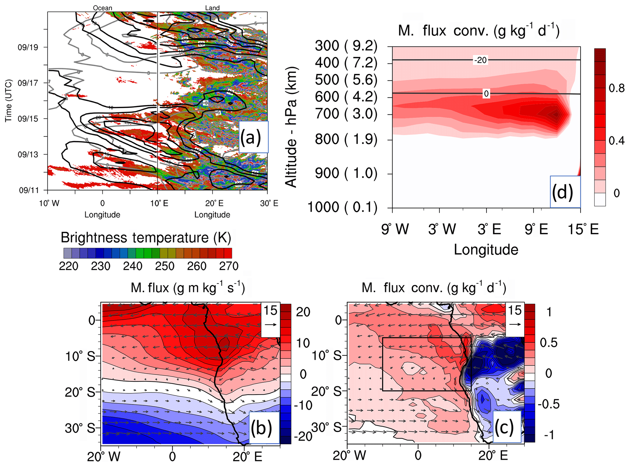
Figure 7 (a) An example showing the longitude–time cross section of brightness temperature (K; shaded), easterly zonal wind speed (gray contours between 3 and 15 m s⁻¹ at 2 m s⁻¹ interval), and moisture flux (black contours between 10 and 30 g m kg⁻¹ s⁻¹ at 5 g m kg⁻¹ s⁻¹ interval) between 3 and 8 km and latitude range of 5–20^∘ S for 11–20 September 2016. The July–October (2006–2010) ERA-Interim (b) moisture flux (g m kg⁻¹ s⁻¹) and (c) moisture flux convergence (g kg⁻¹ d⁻¹), averaged between 3 and 8 km. Positive is convergence, and negative is divergence. The arrows are the moisture flux vectors referenced at 15 g m kg⁻¹ s⁻¹. (d) The longitude–height transect of the moisture flux convergence averaged between 5 and 20^∘ S (black box in c). The horizontal lines in (d) represent the 0 ^∘C and −20 ^∘C isotherms averaged over the same period.

The advection of moisture not yet reaching a relative humidity of 100 % can also generate an isolated mid-level cloud through radiative cooling. High relative humidity within the mid-troposphere can result in increased longwave cooling for the upper part of the layer and contemporaneous warming in the lower part of the layer (e.g., Larson et al., 2006). This differential heating can set off a process that results in turbulent mixing which can redistribute moisture to the upper part of the layer and, in turn, strengthen radiative cooling, thus leading to the development of mid-level clouds. Figure 7d shows the vertical distribution of the offshore moisture flux convergence. Strong convergence of moisture and the potential for strong turbulence and instability directly below the 0 ^∘C level can promote the development of mid-level clouds with tops between the 0 ^∘C and −20 ^∘C isotherm (cf. Fig. 5c and d). Furthermore, it is noteworthy that a smoke layer almost always co-occurs with the mid-level clouds observed during ORACLES-2016 (see Figs. 1, 2, and S2). The presence of the smoke can aid the development of the mid-level cloud through preferential warming in the lower part of the layer (e.g., Adebiyi et al., 2015), thereby strengthening the turbulent mixing within the layer. As a result, the co-occurrence of the moisture and smoke aerosols within the layer serves as an ideal recipe for generating an isolated mid-level cloud characterized by strong mixing within the layer and strong radiative cooling at the top. Whether the cause of particular mid-level clouds is moisture advection or turbulent mixing induced by the longwave cooling of moisture and shortwave absorption by smoke-aerosol layers is beyond the scope of this study. Nevertheless, it is clear that the presence of a high-humidity environment and the associated effect of longwave radiative cooling likely contribute to the development and the eventual sustainability of the mid-level clouds over the southeast Atlantic.

3.4 Radiative impact of the mid-level clouds on the low-level clouds

Because low-level clouds also dominate the southeast Atlantic between July and October, it is useful to examine the radiative impact of the mid-level clouds on the underlying low-level clouds during the same period. Figure 8 shows the low-level-cloud-top instantaneous heating rates obtained from the merged CloudSat–CALIPSO dataset between July and October (2006–2010) when the mid-level clouds are present above the low-level clouds and when they are not. Details of how the heating rates are estimated for the CloudSat–CALIPSO datasets can be found in Henderson et al. (2013) and references therein. Typically the longwave cooling exceeds the shortwave heating near the tops of the low-level clouds when no other higher-altitude clouds are present. Over the southeast Atlantic between July and October, the mean shortwave radiative heating rate at low cloud tops is 5 K d⁻¹, which combines with a longwave cooling rate of −21 K d⁻¹ for a net cooling rate of $\sim -\mathrm{16}$ K d⁻¹ (Fig. 8a).

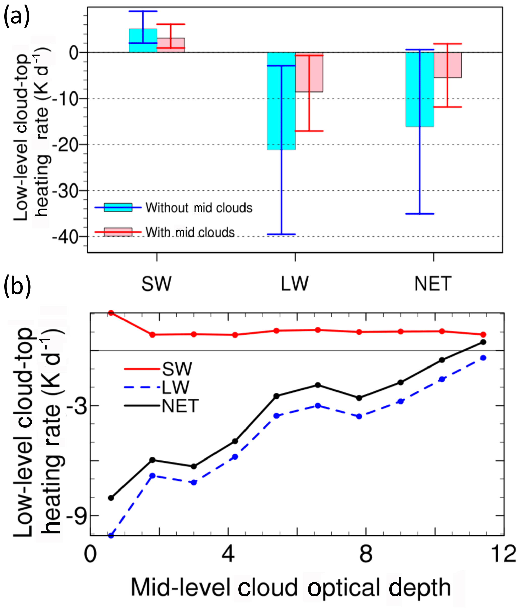
Figure 8 The radiative impact of mid-level cloud on the low-level cloud-top heating rates. (a) The instantaneous heating rates at the top of low-level clouds with (pink bars/red lines) and without (cyan bars/blue lines) the presence of collocated mid-level clouds. (b) The instantaneous heating rates at the top of the low-level clouds as a function of the overlying mid-level cloud optical depth. All data are obtained from the CloudSat–CALIPSO merged dataset between July and October (2006–2010) and over the ORACLES-2016 campaign region (black boxes shown in Fig. 4) and separated into the shortwave (SW) and longwave (LW) components, as well as the NET (NET = SW+LW).

The presence of mid-level clouds over the southeast Atlantic, however, reduces the net radiative cooling substantially at the top of these low-level clouds. In the shortwave, this reduction is due primarily to the decrease in the downwelling radiation reaching the low-level cloud top as a result of the mid-level cloud. Consequently, this leads to an overall reduction in the shortwave heating rate near the top of the low-level cloud of approximately 2 K d⁻¹. In the longwave, the presence of the mid-level clouds increases the downwelling radiation that reaches the top of the low-level cloud, reducing the longwave low-cloud-top cooling rate more substantially by approximately 12.5 K d⁻¹. Thus, the presence of mid-level clouds reduces the net cooling rate near the top of the low-level cloud by approximately 10.5 K d⁻¹, which is approximately a 65 % reduction in the net radiative cooling rates (Fig. 8a).

There is potentially a chance that the mid-level clouds lead to overall warming at the top of the low-level cloud. That is because the downwelling longwave flux reaching the top of the low-level cloud is largely proportional to the mid-level cloud optical depth as long as the cloud is not yet opaque in the infrared. Thus, increases in the mid-level cloud optical depth result in increases in the downwelling longwave fluxes and in decreases in the net radiative cooling rates at the top of the low-level cloud (Fig. 8b). For a sufficiently high mid-level cloud optical depth (∼11), the shortwave heating surpasses the longwave cooling, resulting in net radiative heating rates rather than cooling at the top of the low-level clouds. This is mitigated by the contrasting circulation patterns for the two cloud levels, and further work is required to indicate if a lasting effect is present on the underlying cloud development.

3.5 Diurnal variations of the mid-level clouds

The impacts of longwave radiative cooling, while always present, are more obvious at night when shortwave warming is not occurring. In addition, the indication that the offshore mid-level clouds are associated with moisture detrainment from convection over land, which has a separate distinctive diurnal cycle (Bourgeois et al., 2016), motivates an examination of the diurnal variability of the offshore mid-level cloud and its relationship to that of clouds over land. Figure 9 shows the frequency of occurrence of the mid-level clouds averaged over the ocean (0–10^∘ E) and over the land (10–20^∘ E) obtained from CALIOP and SEVIRI. Over both the ocean and land, more mid-level clouds are observed during the nighttime than daytime. This result is consistent for both CALIOP and SEVIRI, although the frequency of occurrence is significantly lower in the case of SEVIRI because of the difficulty of observing the mid-level clouds (e.g., Fig. 3). Nevertheless, as in the case of Fig. 7a and because of the fine 15 min temporal resolution of the mid-level clouds, we use SEVIRI here only to capture the structure of diurnal variability and not its magnitude. The frequency of occurrence derived from CALIPSO is ∼8 % (28 %) during daytime (nighttime) over land and ∼7 % (12 %) over the ocean, respectively. When accessed at the approximate overpass time of CALIPSO, which is between 12:30 and 13:30 UTC during the day and 00:30 and 01:30 UTC during the night, the ratio of the daytime occurrence to the nighttime occurrence from SEVIRI is approximately 39 % over the ocean. SEVIRI further indicates that the mid-level cloud coverage is at a maximum between 03:00 and 05:00 UTC in the morning and is minimal between 11:00 and 13:00 UTC in the afternoon (Fig. 9b). Furthermore, despite the difference in the frequency of occurrence between daytime and nighttime, the probability distribution of the mid-level cloud-top heights obtained from CALIPSO is largely similar between day and night (see Supplement Fig. S7).

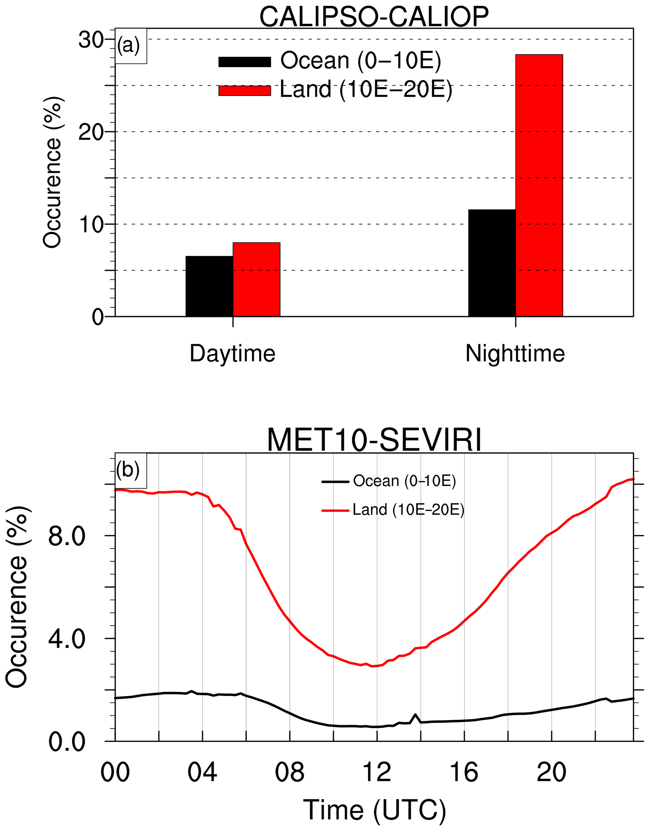
Figure 9 Diurnal variations of the mid-level cloud frequency of occurrence (%) between 3 and 8 km and 1 and 30 September 2016 averaged for 5–20^∘ S, over the ocean (black bar/line; 0–10^∘ E) and the land (red bar/line; 10–20^∘ E) for observations obtained from (a) CALIOP instrument on board CALIPSO and (b) SEVIRI instruments on board the MET-10 satellite. CALIPSO overpass over the southeast Atlantic occurs between approximately 12:30 and 13:30 UTC during the day and 00:30 and 01:30 UTC during the night. Despite SEVIRI's difficulty in identifying mid-level clouds, SEVIRI's higher temporal sampling (15 min) provides insight into the diurnal variability that is otherwise not available.

Overall, the diurnal variability in the amplitude of mid-level cloud occurrence is modulated by the competing influence of the longwave and shortwave radiative heating. The cloud-top longwave cooling and the associated instability are expected to dominate during the night, while the shortwave heating, subsidence, and cloud dissipation are expected to compete with the longwave cooling and possibly dominate during the day. The weaker diurnal cycle over the ocean, coupled with a lower occurrence of the mid-level cloud, is consistent with the presence of less free tropospheric moisture over the ocean than over land and affirms the continent as the source of the offshore moisture.

4 Discussions and conclusions

The southeast Atlantic is an important region because it features one of the major subtropical stratocumulus clouds below one of the most extensive elevated smoke-aerosol layers in the world. While much attention has focused on the low-level stratocumulus clouds due to their spatial extent, persistence through the annual cycle, and regional climate impacts, as well as the aerosol–cloud interactions that are associated with the elevated smoke aerosols, no study has yet focused on the characteristics of the mid-level clouds that also occur over the southeast Atlantic. The presence of mid-level clouds over this region could complicate the evaluation of regional cloud radiative effects and the region's contribution to the global radiative budget. Previous studies have mostly focused on the characteristics of mid-level clouds over the equatorial and midlatitude regions, with little attention given to mid-level clouds over the subtropical regions. Here we document the characteristics of the mid-level clouds over the southeast Atlantic stratocumulus cloud region using a combination of aircraft and satellite observations, as well as reanalysis datasets.

Our analysis primarily relies on the observations of the mid-level clouds collected during September 2016 of the NASA ORACLES field campaign on board the NASA ER-2 aircraft. The ER-2 aircraft, capable of reaching above 20 km in altitude, hosted a High Spectral Resolution Lidar 2 able to observe the entire vertical column of the atmosphere, as well as a scanning polarimeter whose retrievals of the mid-level clouds could be characterized separately from the underlying low clouds. In tandem, these instruments provided a unique view of the multilayer cloud over the southeast Atlantic. These aircraft-based measurements are extended with satellite observations that include the retrievals of cloud properties from CALIPSO and CloudSat–CALIPSO merged datasets between 2006 and 2010, as well as cloud observations from the Meteosat-10 Second Generation (MET10) geostationary satellites and environmental variables from the ERA-Interim dataset.

Our result shows that the mid-level clouds over the southeast Atlantic are relatively common with cloud-top heights typically placed between 5 and 7 km. Measurements from the HSRL-2 indicate that about 93 % of the mid-level clouds observed during the ORACLES campaign are above 5 km. Between 2006 and 2010, the CALIOP-derived mid-level clouds indicate that the majority (about 61 %) of the mid-level cloud-top heights are similarly found between 5 and 7 km altitude, indicating the preferred altitude layer for the mid-level clouds. In addition, the monthly averaged CALIOP frequency of occurrence indicates that the mid-level clouds are mostly prevalent between August and October, with the maximum occurring in September (approximately 15 % of the time) and the minimum in June (∼2 % of the time). The results further indicate that the frequency of occurrence over the southeast Atlantic is highest near the coastal region, up to 30 %, with a gradual decrease westward when averaged between July and October (2006–2010). This period of maximum occurrence of the mid-level clouds also corresponds to the period when the elevated smoke-aerosol loading and the low-level cloud fraction maximize over the southeast Atlantic. This co-occurrence thus highlights the significance of mid-level clouds in influencing the radiative impacts both within the smoke layer and on the underlying low-level clouds over the region. Furthermore, our analysis shows that the aerosol extinctions immediately below the mid-level clouds are typically markedly higher than those above it, suggesting that the mid-level clouds tend to mostly occur at the top of the moist, smoke-aerosol layer.

Between July and October, our results indicate that the mid-level clouds over the southeast Atlantic are optically thin and are characterized by supercooled liquid-water clouds. Specifically, about 64 % of the mid-level clouds have a cloud thickness that is less than 1 km (about 85 % for a thickness of less than 1.5 km), and about 60 % have a cloud optical depth that is less than 4 (72 % for an optical depth of 6). In addition, the probability distribution of the temperature of the mid-level clouds shows that they occur predominantly between 0 and $\sim -\mathrm{20}$ ^∘C. Indeed, the temperature distribution collocated with HSRL2-observed mid-level clouds during the September 2016 ORACLES campaign indicates that more than 98 % of the clouds have a temperature between 0 and $\sim -\mathrm{20}$ ^∘C, which is also comparable with the percentage of mid-level clouds below 0 ^∘C (87 %) that are collocated with the merged CloudSat–CALIPSO datasets between July and October (2006–2010). Despite the cold temperature range, mid-level clouds observed by HSRL-2 and CALIOP instruments during September 2016 places the 532 nm depolarization–backscatter relationships within the signature expected for liquid-water clouds, suggesting no presence of ice in the mid-level clouds over the southeast Atlantic. Furthermore, the effective radius obtained from the Research Scanning Polarimeter (RSP) instrument on the ER-2 aircraft shows that the mid-level cloud droplet sizes are small (median effective radius of ∼5.2 µm) – smaller than those obtained for underlying low-level liquid-water clouds – and with no dependency on the mid-level cloud-top heights, thus discouraging the likelihood of precipitation, either ice or liquid, from within the mid-level clouds.

The mid-level clouds over the southeast Atlantic are mostly associated with synoptically modulated continental moisture outflow which can be linked to the detrainment from the continental convective clouds. Analysis of ERA-Interim reanalysis indicates a strong moisture convergence offshore that can be associated with the deep-layer moisture of the convective regime over the Congo–Zaire basin and a strong mid-tropospheric zonal wind associated with the southern African easterly jet (Adebiyi and Zuidema, 2016) over the southeast Atlantic. In addition, we also highlighted the possibility that the mid-tropospheric high-humidity layer, in the presence of smoke aerosols, over the southeast Atlantic can generate an isolated mid-level cloud due to turbulent mixing within the layer encouraged by strong longwave radiative cooling at the top of the layer. The impacts of radiative cooling, while always present, are more obvious at night when shortwave warming is not occurring. Indeed, the merged CloudSat–CALIPSO dataset shows that the mid-level cloud frequency of occurrence averages ∼12 % during nighttime over the ocean (5–20^∘ S, 0–10^∘ E) compared to only about 7 % during the daytime. The overall diurnal variability over the ocean is consistent with that over land, with the maximum occurring between 03:00 and 05:00 UTC in the morning and minimum occurring between 11:00 and 13:00 UTC in the afternoon.

The presence of these mid-level clouds impacts the radiation reaching the top of the underlying low-level clouds. Between July and October, our analysis shows the presence of the mid-level clouds results in approximately a 2 K d⁻¹ reduction in the shortwave heating rates and ∼12.5 K d⁻¹ reduction in the longwave cooling rates near the top of the underlying low-level clouds. The reduction in the net cooling rate is mainly due to the increase in downwelling longwave radiation from the mid-level clouds. Overall, a 10.5 K d⁻¹ reduction in the net radiative cooling rates associated with the presence of the mid-level clouds accounts for approximately a 65 % reduction when compared to the case without overlying mid-level clouds. The radiative impact of mid-level clouds on the underlying low-level clouds depends on many factors, including the mid-level cloud-top heights, the cloud-base heights, cloud optical depth, temperature, and the microphysical compositions of the mid-level clouds. It also depends on the concentration of smoke aerosols that is between the mid-level and low-level clouds. The low cloud-top radiative cooling rates decrease almost proportionally with increases in the mid-level cloud optical depth. Beyond a mid-level cloud optical depth of ∼11, the shortwave heating rates surpass the longwave cooling rates, leading to net radiative heating rather than cooling, near the top of the low-level clouds. The implication of the reduced net radiative cooling, or the net radiative warming, near the top of the low-level clouds is that the presence of mid-level clouds should facilitate a decrease in turbulent mixing within the boundary layer, all else being equal. This must be weighted by the amount of time the mid-level cloud is present over a particular low cloud scene.

The radiation reaching the surface or the top of the atmosphere will be impacted by the presence of the mid-level clouds despite the presence of the elevated smoke and the low-level clouds. Furthermore, while our analysis highlighted that the aerosol extinction coefficients are higher below the mid-level clouds than above it, it does not examine the potential influence of the smoke-induced shortwave warming on the development, dissipation, or lifetime of the mid-level clouds over the region. The presence of elevated smoke aerosols below (or around) the mid-level clouds strongly points to the potential for aerosol–cloud interaction in the cold environment, which is consistent with the small effective radii retrieved from the RSP measurements.

The prevalence of the multilayer cloud system over the southeast Atlantic highlighted in this study could provide the needed guidance for future remote-sensing retrieval and any modeling efforts over the region. For example, the presence of the mid-level clouds must be accounted for in the observed top-of-the-atmosphere radiance received by the passive remote-sensing platforms (e.g., Peers et al., 2019), as well as in the resulting retrieval of low-level cloud properties, including the low-level cloud-top heights over the region. In addition, the result that the southeast Atlantic mid-level clouds are supercooled liquid-water clouds could help reduce potential uncertainty associated with the cloud-phase representation within models (e.g., Zhang et al., 2005; Barrett et al., 2017). The mid-level clouds occur within a coupled land–atmosphere–ocean system and provide insight into the regional dynamics. Overall, the knowledge of the mid-level cloud properties over the southeast Atlantic could be useful to accurately simulate its radiative effects in the mid-troposphere, its impact on the underlying low-level clouds as a natural laboratory for aerosol–cloud interaction, and the regional cloud radiative budget.