the Creative Commons Attribution 4.0 License.
the Creative Commons Attribution 4.0 License.
 | 14 Sep 2020
Retrieving tropospheric NO2 vertical column densities around the city of Beijing and estimating NOx emissions based on car MAX-DOAS measurements
Xinghong Cheng
Junli Jin
Junrang Guo
Yuelin Liu
Jida Peng
Xiaodan Ma
Minglong Qian
Qiang Xia
Peng Yan
We carried out 19 city-circle-around car multi-axis differential optical absorption spectroscopy (MAX-DOAS) experiments on the 6th Ring Road of Beijing in January, September, and October 2014. The tropospheric vertical column densities (VCDs) of NO2 were retrieved from measured spectra by the MAX-DOAS technique and used to estimate the emissions of NOx () from urban Beijing during the experimental periods. The offline LAPS-WRF-CMAQ model system was used to simulate the wind fields by assimilation of observational data and calculate the NO2-to-NOx concentration ratios, both of which are also needed for the estimation of NOx emissions. The NOx emissions in urban Beijing for the different months derived from the car MAX-DOAS measurements in this study were compared to the multi-resolution emission inventory in China for 2012 (MEIC 2012). Our car MAX-DOAS measurements showed higher NO2 VCD in January than in the other two months. The wind field had obvious impacts on the spatial distribution of NO2 VCD, with the mean NO2 VCD along the 6th Ring Road typically being higher under the southerly wind than under the northerly wind. In addition to the seasonal difference, the journey-to-journey variations of estimated NOx emission rates () were large even within the same month, mainly due to uncertainties in the calculations of wind speed, the ratio of NO2 and NOx concentration, and the decay rate of NOx from the emission sources to the measured positions under different meteorological conditions. The ranges of during the heating and non-heating periods were 22.6×1025 to 31.3×1025 and 9.6×1025 to 12.0×1025 molec. s−1, respectively. The average values in the heating and non-heating periods were molec. s−1 and molec. s−1, respectively. The uncertainty range of was 20 %–52 %. The monthly emission rates from MEIC 2012 are found to be lower than the estimated , particularly in January. Our results provide important information and datasets for the validation of satellite products and also show how car MAX-DOAS measurements can be used effectively for dynamic monitoring and updating of the NOx emissions from megacities such as Beijing.
- Article
(5637 KB) - Full-text XML
-
Supplement
(1431 KB) - BibTeX
- EndNote


Over the past decade, serious haze events have occurred frequently in fall and winter in Beijing due to massive anthropogenic emissions from the combustion of fossil fuels and other sources (He et al., 2013; Zhang et al., 2013). High concentrations of aerosol particulate matter with dynamic diameters less than 2.5 µm (PM2.5) threaten public health (Cao et al., 2014), disturb traffic operation by affecting visibility, and result in perturbations to the weather and climate by scattering and absorption of solar radiation (Liao et al., 2015; Cheng et al., 2017). Measurements have shown that organic matter (OM), sulfate, nitrate, and ammonium made up more than 78 % of the PM2.5 in Beijing during January 2013 (Huang et al., 2014). Fractions of nitrate in PM2.5 have increased recently with the control of industry and coal in the Beijing–Tianjin–Hebei region, which has reduced SO2 emissions and the ratio of sulfate in PM2.5, while traffic emissions are still at high levels. A recent study based on the aerosol observations at the campus of Peking University in 2014 revealed that aerosol pollution is nitrate-driven in spring and early fall and OM-driven in late fall and winter (Tan et al., 2018). The study suggested that nitrate formation was more significant than sulfate formation during severe pollution episodes in Beijing. Therefore, studies on the spatiotemporal variation of NO and NO2 (together denoted as NOx), with the latter being a precursor of nitrate aerosols, are very important for understanding the aerosol formation and its influencing factors.
Emission inventories are usually developed by the so-called bottom-up approach, which is based on combinations of activity statistics (such as energy consumption and industrial production) and source- or region-specific emission factors (Hao et al., 2002; Zhang et al., 2007; Zhao et al., 2012; Streets et al., 2013). However, there are large uncertainties in bottom-up emission inventories associated with the statistics, emission factors, temporal allocation profiles, and grid allocation factors (Ma and Van Aardenne, 2004; Zhao et al., 2012). Moreover, estimating “current” emissions by the bottom-up methodology is fundamentally difficult because publication of basic statistics is generally a couple of years behind. The “top-down” emission estimate is a useful supplement to bottom-up estimates, which are subject to uncertainties in emission factors and emission activities (Streets et al., 2013). Inverse modeling, in which emissions are optimized to reduce the differences between simulated and observed data, is a powerful method that solves the problems of the bottom-up approach. Recently, its application to the estimation of NOx emissions has been widely reported. NOx emission rates are derived by constraining satellite observations using the relationship between model-simulated NO2 vertical column density (VCD) and primary NOx emission estimates from the bottom-up approach (Martin, 2002; Jaeglé et al., 2005; Konovalov et al., 2006; Wang et al., 2007; Lin et al., 2012; Zyrichidou et al., 2015). Nevertheless, errors and uncertainties still exist in the retrieval of satellite data, which leads to a large decrease in the accuracy of estimated emissions, particularly in highly polluted regions such as Beijing and its surroundings (Ma et al., 2013a; Jin et al., 2016). Uncertainties can arise from noise, surface albedo, cloud blocks, profile shape, interference from ozone absorption, correlations with other retrieved parameters, fitting wavelength window, and so forth (Jin et al., 2016; Ma et al., 2013a; Shaiganfar et al., 2011, 2017). Air mass factor (AMF) errors can produce additional errors during the conversion process from the slant to vertical columns. Therefore, comprehensive ground-based measurements of the tropospheric columns and vertical profiles of NO2 are quite important and necessary to evaluate and validate satellite retrieval products.
Multi-axis differential optical absorption spectroscopy (MAX-DOAS) is a ground-based remote-sensing technique developed during the last 2 decades. It makes use of the scattered sunlight measured from the horizontal through zenith-pointing directions to retrieve the VCD and vertical profiles of trace gases and aerosols with relatively high sensitivity in the lower atmosphere (Hönninger et al., 2004; Wagner et al., 2004; Platt and Stutz, 2008). MAX-DOAS has been extensively used to derive tropospheric column information of NO2 and some other pollutants in various regions (Wittrock et al., 2004; Brinksma, et al., 2008; Irie et al., 2008; Vlemmix et al., 2010; Li et al., 2013; Hendrick et al., 2014; Tan et al., 2008; Wagner et al.,2011). Mobile (or car) MAX-DOAS measurements have been used to quantify NOx emissions from cities and regions such as Beijing (Johansson et al., 2008), Mexico (Johansson et al., 2009), Mannheim and Ludwigshafen (Ibrahim et al., 2010), Delhi (Shaiganfar et al., 2011), Shanghai (Wang et al., 2012), and North China (Wu et al., 2018). Compared to ground-based observations at a fixed site, car MAX-DOAS measurements can provide information on the horizontal spatial distribution of pollutants, which is important for explaining the urban/regional representativeness of satellite observations and validating the NO2 VCDs and NOx emission estimates from the new, high pixel resolution measurements by the TROPOMI instrument on Sentinel-5P over megacities such as Beijing. Moreover, due to the rapid expansion of urban areas and increasing energy consumption, both locations and strength of emission sources in Beijing might have changed significantly. Therefore, intensive car MAX-DOAS measurement campaigns are still needed to estimate the emissions of NOx in Beijing. Mean wind speed and wind direction along the ring road during the sampling periods were usually used to estimate NOx emissions in previous studies. Since the wind field changes rapidly due to local circulation and then results in uncertainties in quantification of NOx emissions (Johansson et al., 2008; Shaiganfar et al., 2011, 2017; Davis et al., 2019), refined and accurate simulations of wind fields are needed for the exact emission estimate.
In this study, we estimated the total NOx emissions from urban Beijing based on the VCD of NO2 obtained from intensive car MAX-DOAS measurements on the 6th Ring Road of Beijing in January, September, and October 2014. The offline LAPS-WRF-CMAQ model system with the data assimilation method was used to derive wind speed, wind direction, and NO2∕NOx concentration ratios, which are needed to estimate total urban NOx emissions based on car MAX-DOAS measurements. We attempted to accurately estimate the NOx emission rates and the seasonal difference and deeply investigate the uncertainties and appropriate meteorological conditions for the estimation based on car MAX-DOAS measurements. This paper is organized as follows: Sect. 2 describes the intensive car MAX-DOAS experiments and the retrieval method for deriving tropospheric NO2 VCD, the model system used to simulate the wind fields and the ratios of NO2 and NOx, and the method used to quantify total NOx emissions. Section 3 presents the results of the NO2 VCD and the estimated NOx emissions as well as their uncertainties due to simulated errors in the wind field. Conclusions are provided in Sect. 4.
2.1 Formula to estimate urban NOx emissions
The complete NO2 flux across the urban Beijing area encircled by the driving route S is estimated according to the closed integral method (CIM) of Ibrahim et al. (2010).
Here is the NO2 VCD at the sampling position within the driving route; n indicates the normal vector parallel to the Earth's surface and orthogonal to the driving direction at the position of the driving route; w is the average wind vector within the NO2 layer. We carried out car MAX-DOAS measurements along closed driving routes around large emission sources, i.e., the 6th Ring Road of Beijing (Fig. 1).

Figure 1Driving routes (white dashed line) of the car MAX-DOAS experiment on the 6th Ring Rd of Beijing and distribution of yearly averaged NOx emission rate (mol km−2 h−1) from the MEIC 2012.
We averaged the wind vector data from the Weather Research and Forecasting (WRF) model between surface and 1000 m altitude weighted by the winter exponentially decreasing profiles according to the method of Shaiganfar et al. (2017).
Here w(zi) is the wind vector at altitude zi and z0 indicates the assumed scale height of 300 m for winter.
According to the CIM, the complete NOx emissions from the encircled areas are determined considering the partitioning between NO and NO2 (cL) and the finite lifetime of NOx (cτ).
Here cL is simply the ratio of NOx () and NO2 () bulk concentration in the polluted layer, which are simulated by the Community Multiscale Air Quality Modeling System (CMAQ) model in this study. It is a function of the Leighton ratio (), . To analyze whether there is the impact of VOCs on lifetime of NOx or not, we also calculate another Leighton ratios, Lr, referring to the method of Davis et al. (2019).
where is the NO2 photolysis rate and k8 is the temperature-dependent rate constant for the reaction between NO and O3. We calculate according to the method of Dickerson et al. (1982).
cτ describes the decay of NOx from the emission sources to measured positions. cτ can be estimated from the NOx lifetime τ, which is the reciprocal of the product of reaction rate constant k, OH concentration (COH) and air density (M) (Ma et al., 2013b), and transport time t, which is the distance between emission source and sampling position, r, divided by the wind speed w.
We firstly calculated averaged simulated wind speed and direction, the ratio of NOx and NO2, and the NOx lifetime from surface to 1000 m at every sampling position on the 6th Ring Rd of Beijing for each journey and computed the distance between the sampling position and the center of Beijing for r. Then, we computed cτ, , and . The lifetime τ was calculated with the simulated average OH concentration and air density from surface to 1000 m at each sampling position for each journey.
2.2 Car MAX-DOAS measurements
2.2.1 Instrument and experiment
We measured and retrieved tropospheric NO2 VCD along the sixth ring road of Beijing (hereafter referred to as 6th Ring Rd) in January, September, and October 2014 using a Mini MAX-DOAS instrument mounted on the vehicle.
The instrument, manufactured at Hoffmann Messtechnik GmbH, Germany, is a fully automated, light-weight spectrometer designed for the spectral analysis of scattered sunlight by the MAX-DOAS technique (Hönninger et al., 2004; Davis et al., 2019). The same type of instrument was used in previous studies, including long-term site measurements in Beijing (Ma et al., 2013a) and a car MAX-DOAS observational journey in Europe (Wagner et al., 2010a). The instrument consists of a hermetically sealed metal box of approximately 3 L volume containing entrance optics, a fiber-coupled spectrograph, and all electronics. A spectrometer with the Ocean Optics USB2000+ model is used. A stepper motor, adjusted outside the box, rotates the whole instrument to control the elevation viewing angle. The spectrograph covers the range 292–436 nm and its entrance slit is 50 µm wide. A Sony ILX511 CCD (charged coupled device) detects the light in 2048 individual pixels. The whole spectrograph is cooled by a Peltier stage to guarantee a stable temperature of the optical setup and a small dark current signal. For this study, the instrument was mounted on the roof of a car. Inside the car, two 12 V DC batteries alternatively supplied electronic power for the running of instruments and a laptop computer, with a script run by the DOASIS software (Kraus, 2001) to control the measurement process and the recording of spectra. The temperature of the spectrograph was set to be maintained at −5 ∘C in January and at 0 ∘C in September and October, well below the ambient temperatures during the experimental days of the study. The signal spectra of dark current and electronic offset were measured each day before and after the field experiment on the road, with 10 000 ms and 1 scan for dark current measurements and 3 ms and 1000 scans for electronic offset measurements. Measurements were made alternatively at 30 and 90∘ elevation angles, with every 30∘ measurement immediately followed by a 90∘ measurement. Each elevation angle measurement had an integration time of about 1 min, including typically 300–400 scans for an average spectrum.
The instrument onboard the car was operated to measure scattered sunlight from the driving forward direction. There were no high buildings on both sides of the 6th Ring Rd, and the measurements were made at a wide-field view. The driving speed was typically controlled at 80–90 km h−1, and it generally took about 2.0–2.5 h to complete one circle (about 187 km) around the 6th Ring Rd. Figure 1 shows the driving route of the car MAX-DOAS experiment on a map of Beijing and spatial distribution of the yearly NOx emission rate with a resolution of 0.25∘ × 0.25∘ from the MEIC inventory in 2012, which includes the transportation, power plant, residential, industry, and agriculture sectors. For this study, the field experiments were carried out on 14 selected days, with one or two circling journeys each day. In total, there are 19 circling journeys available. The sampling periods in this experiment and the meteorological conditions are listed in Table 1. The average wind speeds for experimental days in January, September, and October were 2.5, 2.5, and 2.4 m s−1, the corresponding total cloud fractions were 4.9, 7.5, and 4.2, and the mean planetary boundary layer (PBL) heights were 192, 188, and 238 m, respectively. The dominant wind directions in the three months were much more variable, including the northerly, southerly, and other directions and static wind. Since variations of the wind field can affect the estimation of , we synthetically analyze the distribution of the wind field using simulations from the WRF model and reanalysis data with a spatial resolution of 0.125∘ × 0.125∘ every 3 h from the European Centre for Medium-Range Weather Forecasts (ECMWF). In some cases, the wind direction changed slightly within one circling journey period, which is marked as southerly (S) or northerly (N) type in Table 1. However, the wind field during some journeys was convergent or divergent in some areas of Beijing, which is marked as other type (O), and the wind speed was very low in three journeys, which is marked as static type (St). To estimate the NOx emissions accurately using the CIM, the wind speed needs to be sufficiently high, so that the transport across the encircled area is fast compared to the atmospheric lifetime of the trace gas (Ibrahim et al., 2010). In this study, we only consider the circling journeys with a consistent wind field (S or N type) and relatively high wind speed to estimate the NOx emissions. The related information for all the journeys, including 11 selected ones for emission estimation, is given in Table 1.
Table 1Sampling periods of the car MAX-DOAS experiment and corresponding meteorological conditions over Beijing in January, September, and October 2014.
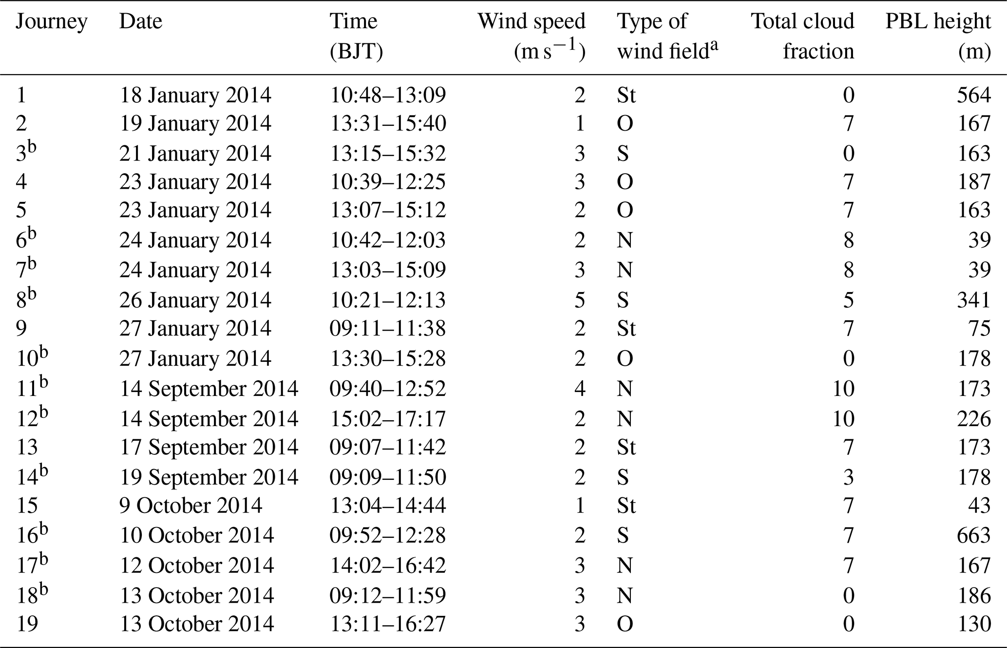
a Four types of wind field are southerly (S), northerly (N), other (O), and static (St). b The data are preliminarily selected to estimate the NOx emissions.
2.2.2 Spectral retrieval
The retrieval of NO2 slant column densities (SCDs) is based on the DOAS method (Platt, 1994). The WinDOAS software (Fayt and Van Roozendael, 2011) was adopted to analyze the spectra in the 400–431 nm range on a daily basis. The Fraunhofer reference spectrum (FRS) was selected among the measured spectra at the 90∘ elevation angle each day by two steps: first, a spectrum measured around noon was chosen; second, the spectrum corresponding to the minimum NO2 SCD derived in the preliminary analysis using the FRS from the first step was finally selected. The absorption cross sections of NO2 at 294 K (Vandaele et al., 1998), O3 at 221 K (Burrows et al., 1999), and the oxygen dimer O4 at 298 K (Greenblatt et al., 1990), as well as a FRS, a Ring spectrum calculated from the FRS by DOASIS (Kraus, 2001), and a polynomial of third order were included in the spectral fitting process. Figure 2 shows an example of our spectral analysis for a measurement on 18 January 2014, 11:39:38 BJT. As shown in the figure, the atmospheric NO2 absorption structure can be clearly extracted from the measured spectra.
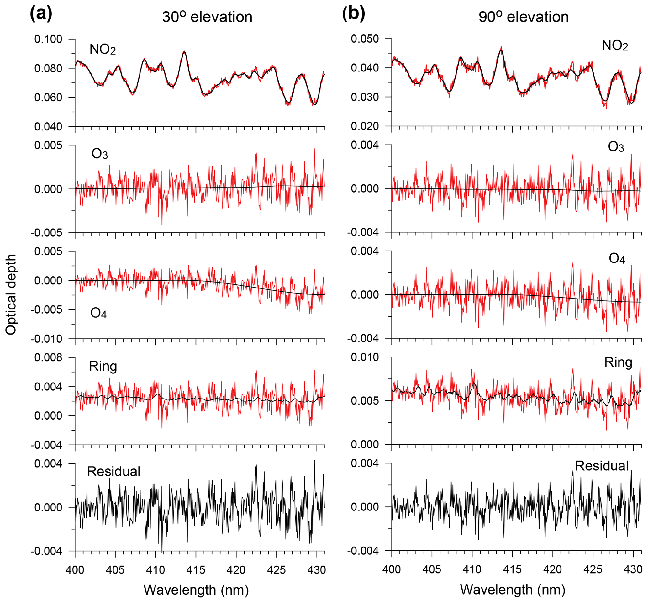
Figure 2Examples of the NO2 retrieval from two successive spectra measured (a) at a 30∘ elevation angle (with NO2 differential slant column density (DSCD) of 1.2×10¹⁷ molec. cm−2) and (b) at a 90∘ elevation angle (with NO2 DSCD of 6.2×10¹⁶ molec. cm−2) on 18 January 2014, at around 11:40 BJT.
2.2.3 Derivation of tropospheric NO2 VCD
The trace gas VCD in the troposphere can be calculated using its SCD divided by the AMF at an elevation angle, α:
For the in situ MAX-DOAS measurements, a FRS from the same elevation sequence was used in most cases, and the stratospheric absorption can be assumed to be the same during one elevation sequence. Therefore, the VCDtrop can be calculated by extending Eqs. (8) to (9) using the so-called differential tropospheric slant column density (DSCD) divided by the differential air mass factor (DAMF):
with DSCD (Wagner et al., 2010b; Ma et al., 2013a).
For the car MAX-DOAS measurements, the trace gas concentrations can change significantly during one measurement sequence, and thus the dependence of retrieved trace gas DSCDs on the elevation angle may not be so regular as for the in situ measurements. Therefore, it would be a better choice to use a single FRS for the analysis of all the spectra measured along the driving route (Wagner et al., 2010b). According to Wagner et al. (2010b), Eq. (9) can be further extended to
where DSCDoffset depends on the solar zenith angle (SZA) and thus local time, ti. For each elevation sequence i during the individual measurement day, DSCDoffset is calculated from a single pair of measurements with
The time series of the calculated DSCDoffset(ti) in this study could be fitted by a low-order polynomial, e.g., , as a function of time. The fitted polynomial then represents the best guess for DSCDoffset and can be used to calculate the VCDtrop from Eq. (10). In this study, the AMF was calculated by the geometric approximation (Brinksma et al., 2008; Wagner et al., 2010b), that is,
As an illustration, Fig. 3 shows the changes in individual NO2 DSCDmeas and DSCDoffset for a 30∘ elevation angle of each sequence as a function of time on 18 January 2014. As shown in Fig. 3, a second-order polynomial fitted from individual DSCDoffset data points as shown in Fig. 3 tends to be stable and can be used to represent an average value of DSCDoffset.
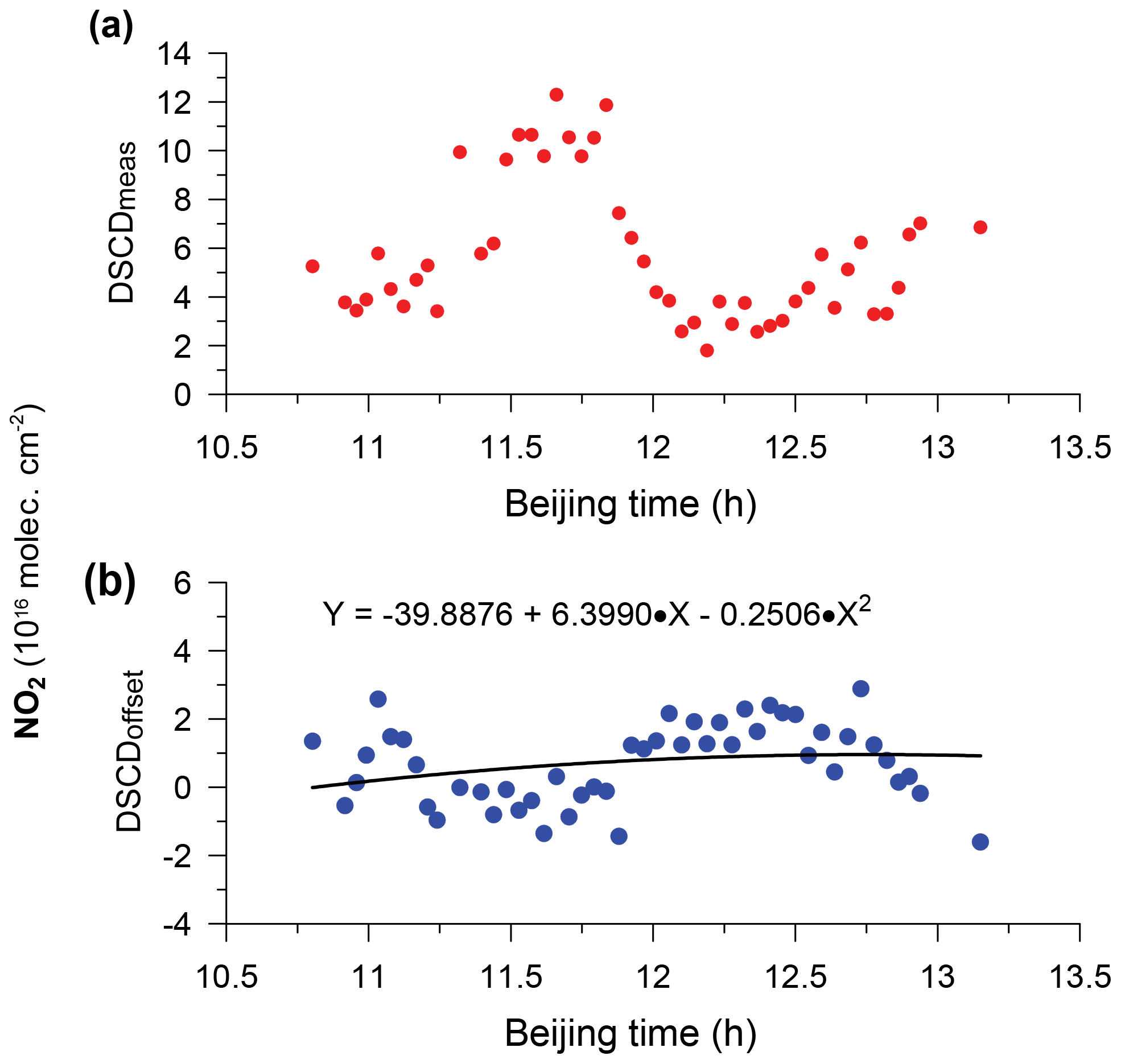
Figure 3Time series of the NO2 (a) DSCDmeans (red dots) and (b) DSCDoffset (black dots) (units of 1016 molec. cm−2) for the 30∘ elevation angle of each sequence on 18 January 2014. The black curve represents a second-order polynomial fit from individual DSCDoffset data points.
2.3 LAPS-WRF-CMAQ model simulation
2.3.1 Model setup and data
To quantify the NOx emissions in Beijing more accurately, refined simulations of the wind field and NO2-to-NOx concentration ratio were needed. In this study, we utilized the offline LAPS-WRF-CMAQ model system with a high spatiotemporal resolution and data assimilation technique to obtain the refined wind speed and wind direction and an accurate ratio of NO2-and-NOx concentration during the car MAX-DOAS experiments. The aforementioned model system includes three components: the Local Analysis and Prediction System (LAPS) model (Albers et al., 1996), the WRF model (Michalakes et al., 2004), and the CMAQ model (Dennis et al., 1996). Simulation of wind speed and direction is improved by the LAPS-WRF model, which assimilates observed data at the surface and high layers using the one-dimensional and three-dimensional variational assimilation methods (Albers et al., 1996). The CMAQ model is used to simulate the temporal–spatial distribution of NO2 and NO concentration. The LAPS, developed by the NOAA Earth System Research Laboratory, is used in many numerical weather forecast centers around the world. It is a mesoscale meteorological data assimilation tool that employs a suite of observations to generate a realistic, spatially distributed, time-evolving, three-dimensional representation of atmospheric structures and processes (McGinley et al., 1991). The three-dimensional realistic meteorological analysis field can be used as the initial condition of the WRF model and improve the simulation of wind fields. WRF is a mesoscale numerical weather prediction system designed for both atmospheric research and operational forecasting needs. CMAQ is an air-quality model developed by the U.S. Environmental Protection Agency's Atmospheric Science Modeling Division. It consists of a suite of computer programs for modeling air quality issues, including reactive gases such as NO2, NO, SO2, O3, and others, particulate matter (PM), air toxins, acid deposition, and visibility degradation.
This study focused on Beijing at a horizontal resolution of 4 km × 4 km with 31 vertical layers of varying thickness (between the surface and 50 hPa) using a triple-nested simulation technique. The horizontal resolutions of the three sets of grids were 36, 12, and 4 km, respectively (Fig. S1a in the Supplement), and the output temporal interval was 1 h. The LAPS-WRF simulations were driven by FNL/NCEP analysis data every 6 h during the car MAX-DOAS experiments, with a spatial resolution of 1∘ × 1∘. In addition, to improve the simulation of wind field and NO2 and NO concentrations, many meteorological data of the same periods, such as wind speed, wind direction, air temperature, and relative humidity, observed at 2400 surface weather stations and 120 radiosonde stations were assimilated into the initial field of the WRF model using the one-dimensional and three-dimensional variational assimilation methods in the LAPS model. The CMAQ model uses the multi-resolution emission inventory in China for the year 2012 (MEIC 2012) with 0.25∘ × 0.25∘ resolution (Zhang et al., 2009; Li et al., 2017). Hourly gridded MEIC emission datasets at a horizontal resolution of 4 km × 4 km for the CMAQ model were generated by the Sparse Matrix Operator Kernel Emissions (SMOKE) modeling system (UNC, 2014) using reasonable temporal and grid allocation factors (Cheng et al., 2017). Meteorological outputs from the WRF simulations were processed to create model-ready inputs for CMAQ using the Meteorology–Chemistry Interface Processor (MCIP) (Otte and Pleim, 2010). The chemical mechanism is CB05, and the boundary conditions of trace gases consist of idealized, Northern Hemispheric, mid-latitude profiles based on results from the NOAA Agronomy Lab Regional Oxidant Model. The model simulation was started 1 d before the first day of the experiment to avoid the spin-up problem and improve the simulation accuracy.
2.3.2 Validation of simulated surface wind and NO2
Modeled wind speeds and directions were validated by observation data from four weather stations in Beijing. Figures S2, S3, and S4 show the scatter distribution between simulated wind speed and observation, the wind rose of modeled wind direction and measurements, and their time serials. We adopted the observed hourly wind speed and direction data from Nanjiao (NJ), Tongzhou (TZ), Mentougou (MTG), and Shunyi (SY) meteorological stations, which represent the southern, eastern, western, and northern areas of Beijing, respectively. It was shown that the temporal variations in simulated wind speed at the four stations were consistent with the observations from the perspective of time serial of wind speed, but the simulations were higher than the observations due to impacts of the complex topography and limited observation data assimilated to the LAPS-WRF model (Figs. S2 and S4a). To calculate the accurately, we corrected the simulated wind speed using the observation data from the four weather stations in order to reduce the systemic error. Specifically, we computed the relative error of the modeled wind speed based on measurements at four weather stations for each journey and then added the error bar to simulated wind speed at every sampling position during the same journey. The correlation coefficient between simulated and observed wind speeds at the four stations is 0.5, and the result passes the 99.9 % significance test. The root mean square error (RMSE) is small, with a value of 1.2 m s−1. Except for the MTG station, simulated wind directions at the other three stations are in accordance with the observations, particularly for the primary wind direction (Figs. S3 and S4b). In general, simulated wind directions are also coincident with observations from the perspective of time serial of wind direction, and simulations are larger than measurements during some periods at some stations due to the effects of the complex topography and limited observation data assimilated to the model (Fig. S4b). The primary wind direction and its frequency at the MTG station are not consistent with the observations because these are affected by the complex topography near the Taihang and Yanshan mountains. In general, the corrected wind speed and wind direction data are reliable for estimation of the NOx emissions, and the uncertainty of due to the variation of the wind field is discussed in Sect. 3.3.
Figure S4 presents the temporal variation in simulated and observed NO2 concentration from 18 January to 13 October 2014. The hourly measurements of NO2 concentrations (shown in Fig. S1b) were obtained from the National Environment Monitoring Station in China. In general, the temporal variation in the NO2 simulation is consistent with the observation. The simulated values are close to the observations, except for 21–24 January, 19 September, and 9–10 October, when NO2 simulations are higher than the observations (Fig. S5). The correlation coefficient between simulated and observed NO2 concentrations is 0.7, and the result passes the 99.9 % significance test (Fig. S6). The RMSE and mean absolute error (MAE) are 16.1 and 19.2 µg m−3, respectively. The observed NO2 might include some NOz component, leading to a systematical bias (underestimation) of NO2 by the model compared to observation (Ma et al., 2012). Thus, the simulated NO2 concentrations and hence the ratio of NO2 and NOx are reliable for estimating NOx emissions.
2.4 Selection of the journeys for estimating NOx emissions
To estimate the NO2 fluxes () and accurately, we firstly selected six journeys with the RMSEs of simulated wind speeds at the four weather stations smaller than 1.5 m s−1 from the primary selected 11 journeys. Then we assessed whether the meteorological and chemical conditions meet the criteria of Shaiganfar et al. (2017) for each of these six journeys or not. It should be pointed out that we cannot assess the problem of a large partitioning ratio due to the absence of the whole seasonal simulated or observed data in fall and winter. The assessment results of the other four problems are listed in Table 2. We excluded the journeys in which more than two problems occurred. It needs to be noted that lifetime correction coefficients cτ on 12 and 13 October are slightly larger than 1.5, which is the criterion of a large lifetime correction (Shaiganfar et al., 2017), so we also adopted the data on 12 and 13 October to estimate the . Lastly, NO2 VCD measurements outside of the 6th Ring Rd during five selected journeys were not used to quantify and .
Table 2Overview of the problems for the six circling journeys.
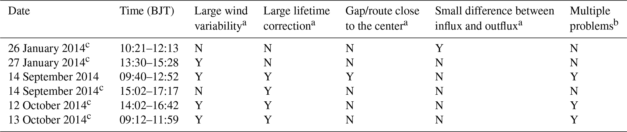
a Whether the condition meets the criteria of Shaiganfar et al. (2017) or not, Y and N denote Yes and No, respectively. b Multiple problems mean whether more than two conditions can meet the criteria or not. c The data of five circling journeys are ultimately used to estimate the NOx emission.
3.1 Tropospheric NO2 VCD
Figure 4 presents the journey-to-journey temporal variation in the tropospheric NO2 VCD on the 6th Ring Rd of Beijing in January, September, and October 2014. In general, the NO2 VCD in January was higher than that in the other months. The highest values occurred on 19, 23, and 24 January. The mean NO2 VCD ranged mostly from to molec. cm−2 in January, but values were all lower than 4.5×10¹⁶ molec. cm−2 in September and October. The NO2 VCD values during the mornings of 23 January and 13 October were 9.1×10¹⁶ and 1.2×10¹⁶ molec. cm−2, corresponding to the maximum and minimum values, respectively, during the 19 circling journeys. This result might be caused by higher emissions from coal-fired heating (Table S1 in the Supplement) and lower photolysis of NO2 in winter. A similar pattern of seasonal variation in tropospheric NO2 VCD was found previously by site MAX-DOAS measurements in Beijing (Ma et al., 2013a; Hendrick et al., 2014).
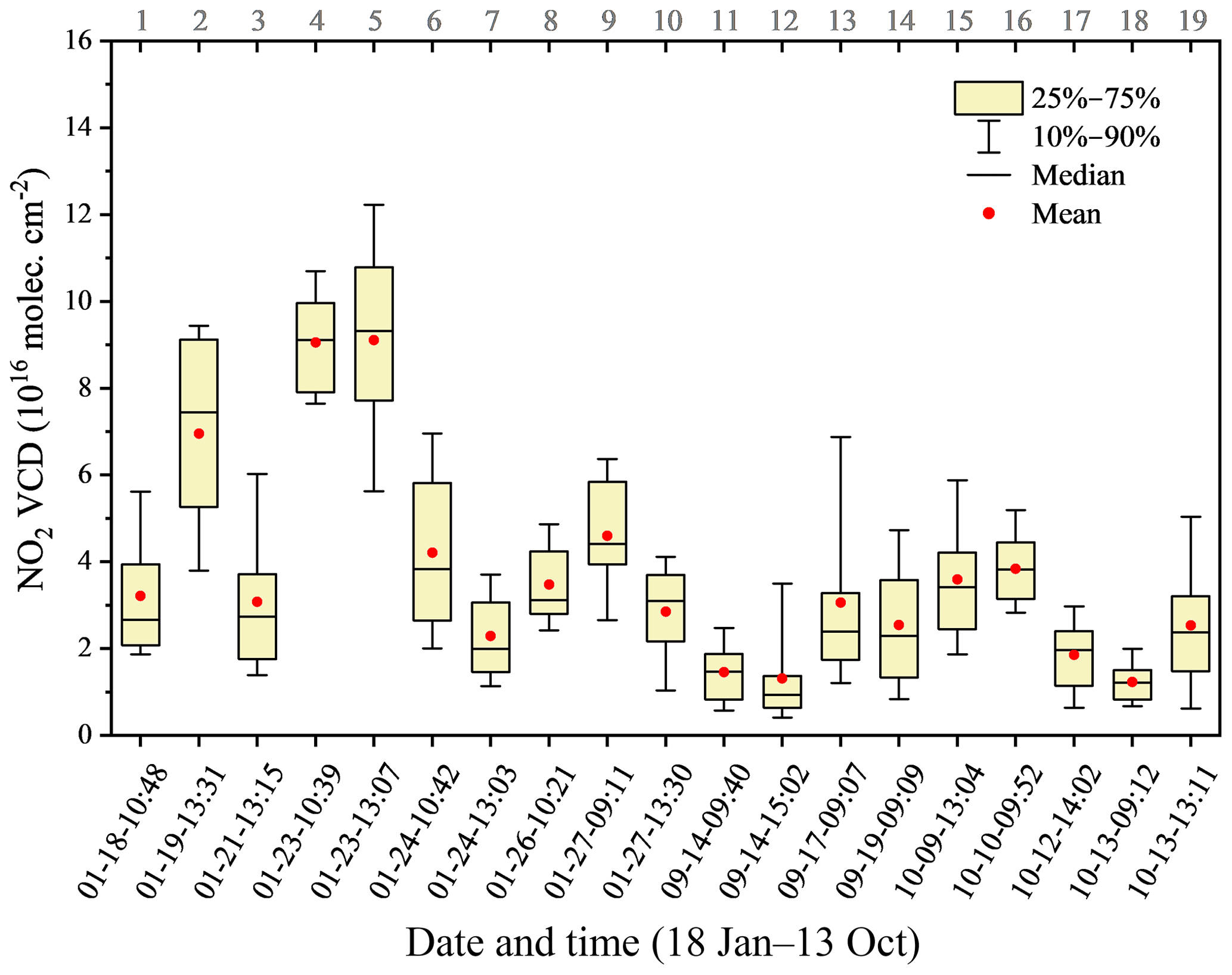
Figure 4Time series of the tropospheric NO2 vertical column density (VCD) for 19 circling journeys on the 6th Ring Rd of Beijing in January, September, and October 2014. Lower (upper) error bars and yellow boxes are the 10th (90th) and 25th (75th) percentiles of the data of each journey, respectively. Hyphens inside the boxes are the medians, and red circles are the mean values. The numbers of each journey are labeled on the top axis. See Table 1 for detailed information about each journey.
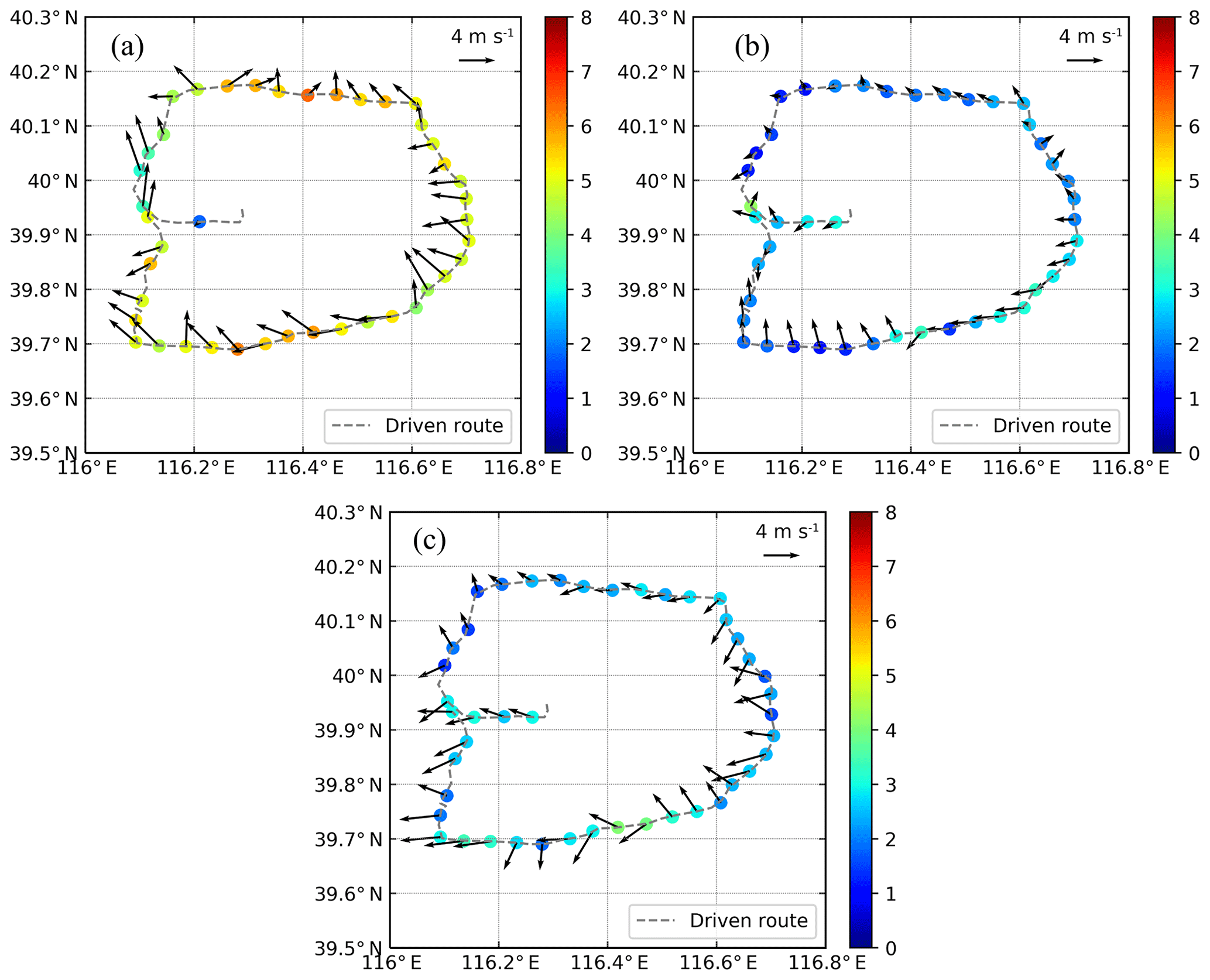
Figure 5Distributions of monthly averaged NO2 VCD (1016 molec. cm−2) on the 6th Ring Rd of Beijing in (a) January, (b) September, and (c) October 2014.
To investigate the differences in the spatial distribution of NO2 VCD among the three months, we computed the monthly average NO2 VCD for every sampling position along the 6th Ring Rd of Beijing in January, September, and October 2014 (Fig. 5). Firstly, we used the locations of all sampling positions in the morning of 23 September as the reference point for the calculation of NO2 VCD monthly average, with the most sampling sites (98 points) for all observation periods. Then, we calculated the monthly average value at each reference point using the data of the nearest sampling position. The distance from the nearest sampling position to a reference point was less than 1.5 km. Figure 5 shows that the monthly average NO2 VCD values at most sampling points on the 6th Ring Rd were obviously larger in January than in the other two months (by a factor of 2 in most cases). The spatial distribution characteristics of NO2 VCD in September were similar to those in October. In addition, the NO2 VCD values in the northern and southern parts of the 6th Ring Rd were all larger than those in the other areas for all three months. The high NO2 VCD in the southern region was related to strong local emissions to the south of Beijing and transport from central and southern Hebei and the city of Tianjin (Meng et al., 2018). As shown in Fig. 4, the maximum journey-averaged NO2 VCD occurred on the morning of 23 January, and the minimum occurred on the morning of 13 October.
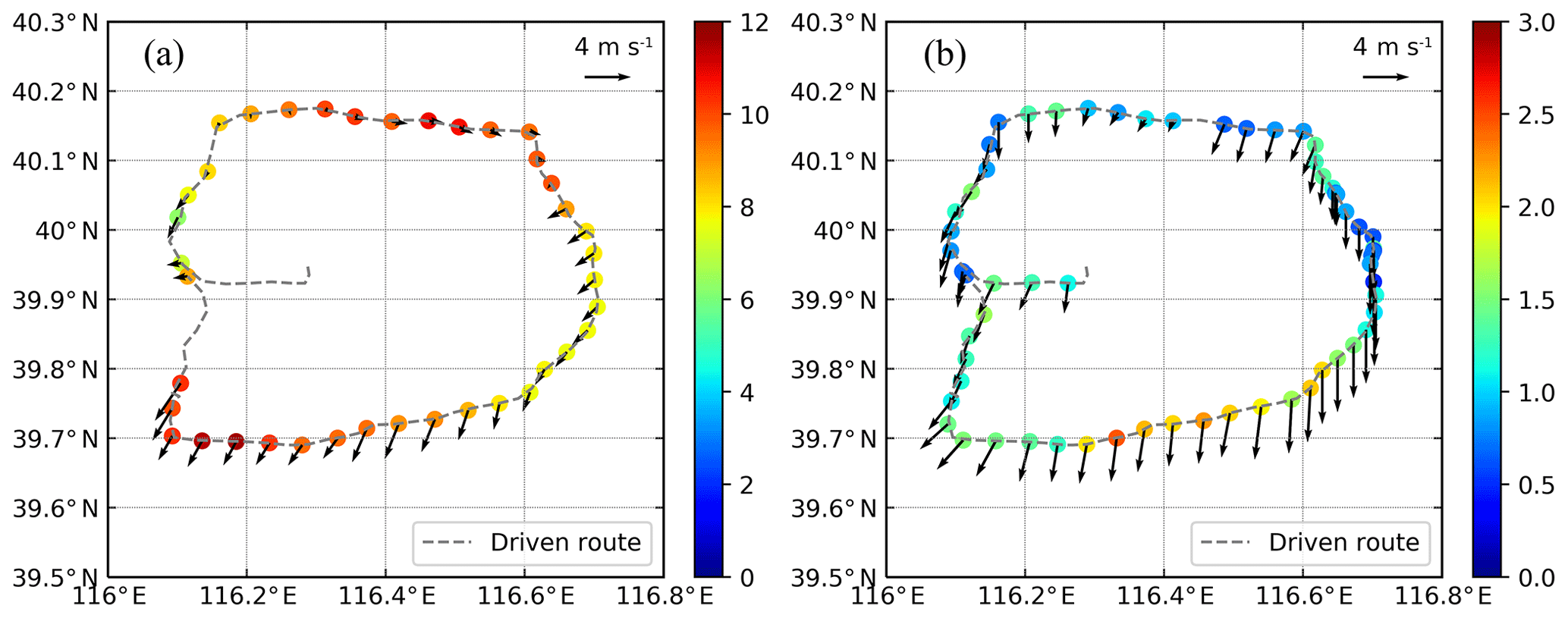
Figure 6Distributions of the maximum and minimum NO2 VCD (1016 molec. cm−2) on the 6th Ring Rd of Beijing on the morning of (a) 23 January and (b) 13 October 2014.
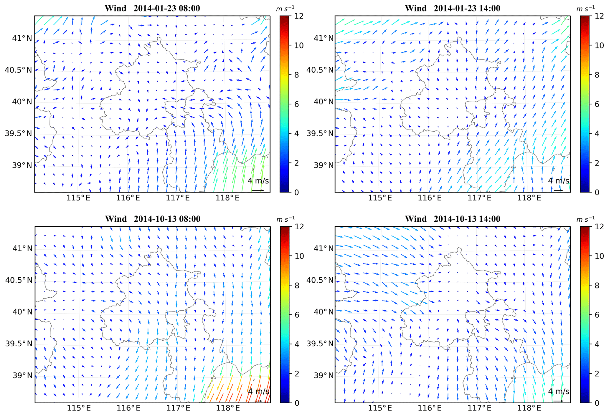
Figure 7Wind fields in Beijing and the surrounding area from the ECWRF at 08:00 (left column) and 14:00 (right column) BJT on 23 January and 13 October 2014.
We investigated the spatial distribution differences in NO2 VCD between these two circling journeys, as shown in Fig. 6. The NO2 VCD values on the 6th Ring Rd in the morning of 23 January were all large, particularly in the northern and southwestern areas, with magnitudes of 10×1016 to 12×1016 molec. cm−2. On 13 October, high NO2 VCD was located in the southern areas, and it might be related to the southern emission sources closer to the southern 6th Ring Rd, where its emission rates are obviously higher than the northern Ring Rd. The spatial distribution differences between these two journeys were related to the high emission during the heating season in January (see Sect. 3.2) and the impacts of the wind field. We used thin-grid ECWMF reanalysis data for 23 January and 13 October with a spatial resolution of 0.125∘ × 0.125∘ to investigate the impact of the wind field on the spatial distribution of NO2 VCD. Figure 7 shows the wind fields at 08:00 and 14:00 BJT on these two days, respectively. The NO2 VCD was large, with weak southerly wind and convergence of southeasterly and northwesterly wind in Beijing and its surrounding area, but its values were far smaller, with strong northerly wind. Weak southerly wind and a breeze or calm wind resulted in the transport of NO2 from the southern area in Hebei Province and its accumulation on 23 January. Strong northerly wind suppressed the transport of NO2 from the southern area on 13 October. These results indicate that the wind field has large impacts on the spatial distribution of NO2 VCD in Beijing.
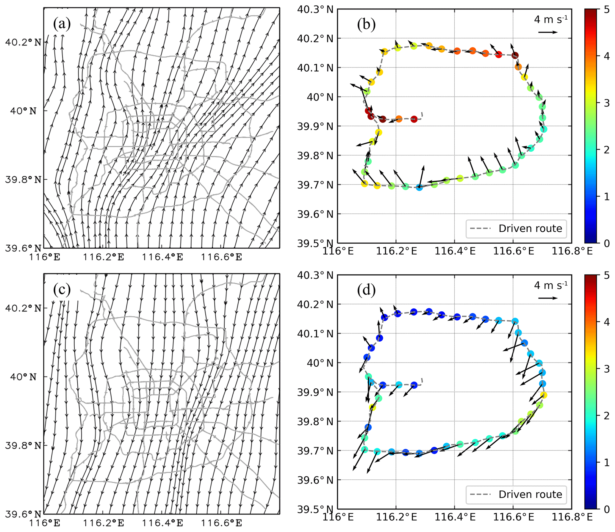
Figure 8Average wind stream and NO2 VCD (1016 molec. cm−2) distributions under the two different types of wind field over Beijing: (a) southerly wind, (b) NO2 VCD under southerly wind, (c) northerly wind, and (d) NO2 VCD under northerly wind.
Figure 8 presents the spatial distributions of wind and NO2 VCD averaged for the two different wind fields. The mean NO2 VCD at most sampling positions along the 6th Ring Rd was obviously higher under the southerly wind field than the northerly wind. High NO2 emission sources were located within the 5th Ring Rd of Beijing in the three months (Fig. 10), and the background concentrations of NO2 VCD in the northern and southern areas were remarkably different due to the impacts of emission sources on the south of Beijing. Hence, southerly wind can transfer air pollutants from the southern area to Beijing and lead to high NO2 flux, whereas impacts of northerly wind on NO2 flux are smaller because the background concentrations of NO2 VCD in the north of Beijing were lower. Convergence of the wind field in the southern parts of the 6th Ring Rd is favorable to the accumulation of NO2 from the surrounding area to the southern parts of the ring road.
3.2 Quantification of NOx emissions
Figure 9 shows the journey-to-journey variation of the estimated and over Beijing for five circling journeys in January, September, and October 2014. The fell in between 1.9×1025 and 15.7×1025 molec. s−1. The ranges of during the heating (January) and non-heating (September and October) periods were 22.6×1025 to 31.3×1025 and 9.6×1025 to 12.0×1025 molec. s−1, respectively. The average values in the heating and non-heating periods were and molec. s−1, respectively. In general, the journey-to-journey variation patterns of and are consistent with that of the mean NO2 VCD. In other words, the estimate of is determined mainly by the NO2 VCD. Seasonal variation characteristics of the estimated were obvious. Specifically, the total was higher in January than in the other two months. The average in the heating period was about 2.5 times as much as those in the non-heating period. The coal-fired heating in Beijing included central heating in the urban area and scattered coal combustion in the suburbs or rural area for the year 2014. We calculated the average NOx emission rates of four sectors, including industry, power, residential, and transportation, from the MEIC within the 6th Ring Rd of Beijing in January, September, and October 2012 and the ratio of each specific NOx emission rate in January to the corresponding average value in September and October (Table S1). The from the power and residential sections was remarkably higher in January than in the other two months, and especially from the residential sector was in January 5.4 times as much as those in the other two months. In general, central heating in the urban area is from power plant and residential use of the scattered coal combustion in the suburbs or rural area.
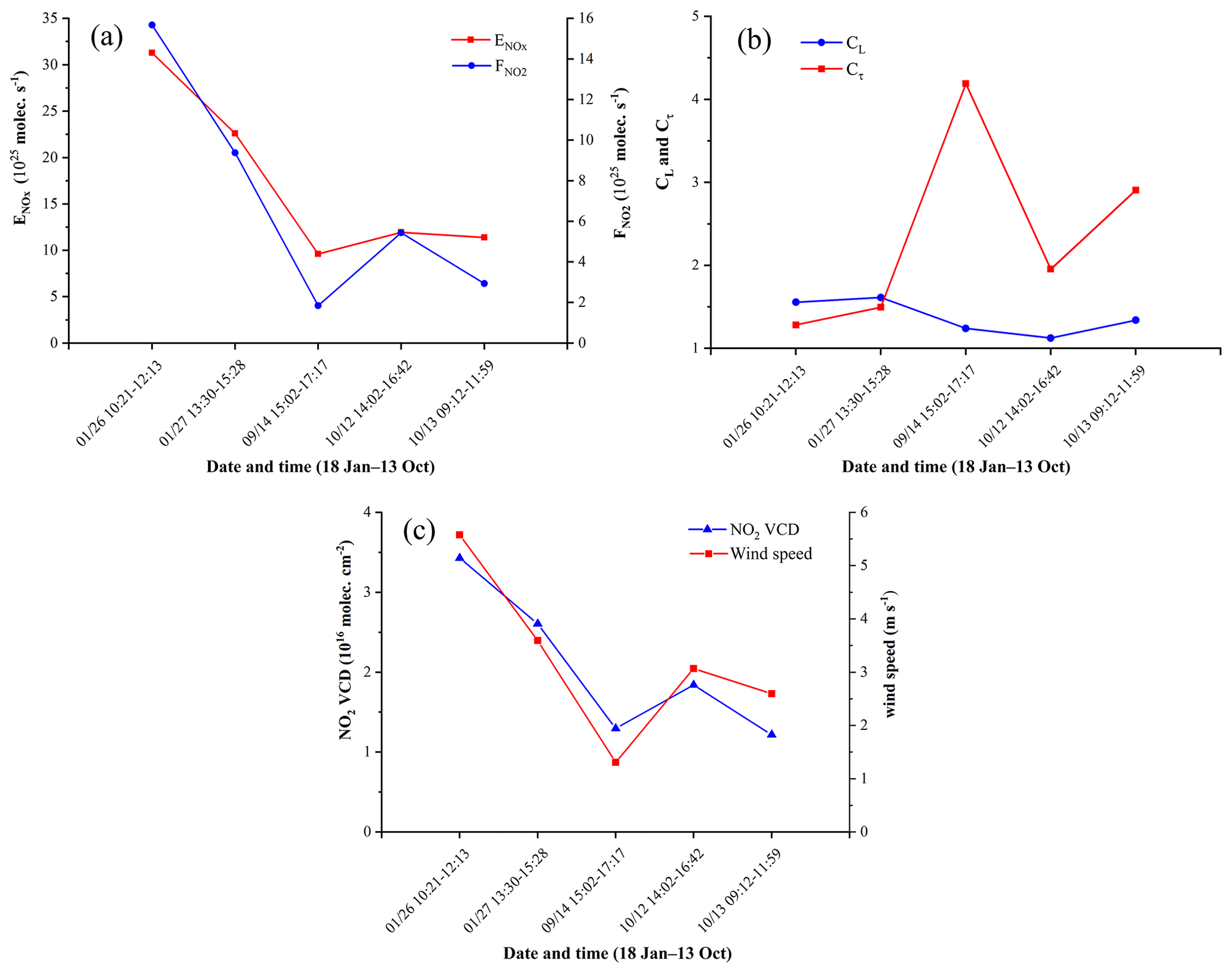
Figure 9Journey-to-journey variations in (a) and , (b) cτ and cL, and (c) NO2 VCD and mean wind speed for five circling journeys on the 6th Ring Rd of Beijing in January, September, and October 2014.
In addition to the seasonal differences, the journey-to-journey variation in estimated is large even within the same month, mainly due to uncertainties in the calculations of wind speed, the ratio of NO2 and NOx concentration, and the decay rate of NOx from the emission sources to the measured positions under different meteorological conditions. In addition to the NO2 VCD, wind speed, and wind direction at the sampling positions, the estimated NOx emission rate is obviously affected by the Leighton ratio of NO and NO2 concentration and the lifetime of NOx (Valin et al., 2013). Thus, the estimated NOx emission rate could be very large even if the NO2 VCD was small, such as in the case of 14 September. It should be noted that the low mean wind speed on 14 September leads to high cτ, so the for this journey is not too small, although the was very low. In addition, if both cτ and cL are large, high can be derived.
3.3 Comparisons with the MEIC inventory
We compared the estimated NOx emission with the MEIC 2012 (Zhang et al., 2009, 2012). The horizontal resolution of MEIC 2012 is 0.25∘ × 0.25∘, and five sectors, i.e., agriculture, industry, power, residential, and transportation, are included.
Figure 10 presents the spatial distributions of NOx emission rates from MEIC over Beijing in January, September, and October 2012. A high NOx emission zone was located within the 5th Ring Rd of Beijing, and low emissions occurred in its surroundings. The NOx emissions in January were obviously larger than those in the other two months.
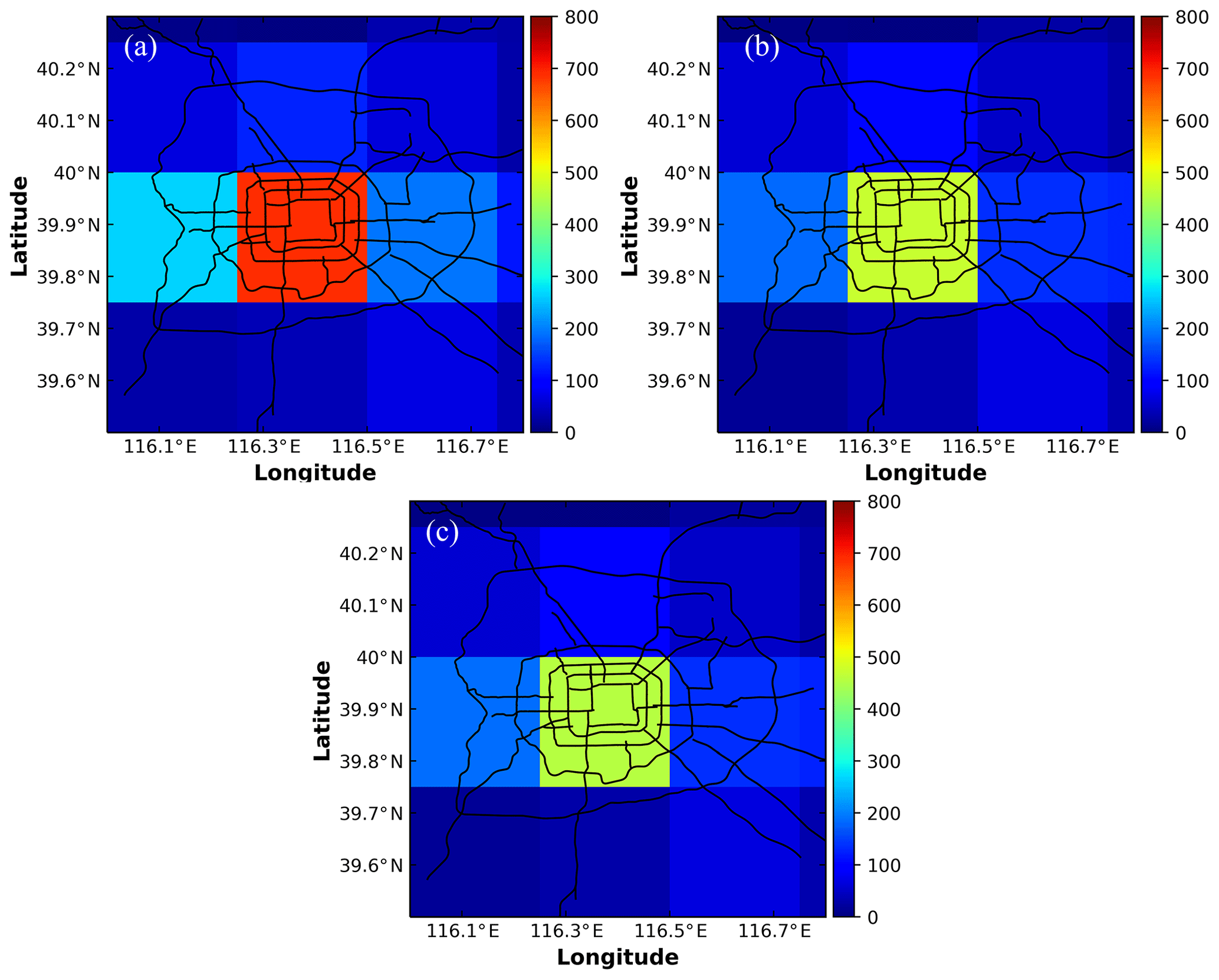
Figure 10Spatial distributions of monthly averaged NOx emission rate (mol km−2 h−1) over Beijing based on the MEIC inventory in (a) January, (b) September, and (c) October in 2012.

Figure 11Journey-to-journey variations in estimated and corresponding monthly emission rate from the MEIC inventory (MEIC_Month) within the 6th Ring Rd of Beijing in January, September, and October 2014. Error bars represent the uncertainties in estimated .
Figure 11 shows the estimated NOx emission rates from car MAX-DOAS measurements for each selected journey (see Sect. 2.4) in January, September, and October 2014 and the corresponding monthly averaged NOx emission rates from the MEIC 2012 for the same region within the 6th Ring Rd of Beijing (hereafter expressed as MEIC_Month). The MEIC_Month is obviously lower than the estimated in January. While the two emission estimates are very close in September, the MEIC_Month is slightly smaller than the in October. The differences between the estimated and the MEIC_Month during some journeys were remarkably large, which may be caused by (1) the interannual variations in the emission inventory, (2) the different timescales of the two emission estimates, and (3) the uncertainty of the estimated and MEIC 2012. Firstly, the in this study is estimated for the year 2014, whereas the MEIC_Month was established for the year 2012. Secondly, our results represent only the conditions during a few measurements in the daytime, whereas the MIEC 2012 denoted monthly average conditions. Thirdly, the uncertainty of the MEIC 2012 is large, particularly in fall and winter (Li et al., 2017; Meng et al., 2018). There are also large uncertainties in the estimated caused by, e.g., the inconsistency of the wind field during a circling journey and the transfer of NO2 from other source areas than urban Beijing. The CIM assumes that the wind field is constant during the measurement period and that the wind speed is also sufficiently high. However, the wind field during some journeys (27 January and 12 and 13 October) might have changed systematically. Ibrahim et al. (2010) also pointed out that systematic changes during the measurements period can have large impacts on the emission estimate, particularly if measurements with high trace gas VCD are accompanied by strong deviations of the actual wind speed (or direction) from the assumed average values. For example, on the afternoon of 27 January, high NO2 VCD was measured, and the wind field changed during the measurement journey. In such cases, the systematic changes in wind speed and direction can lead to additional uncertainties in . Moreover, because the southerly wind can bring NOx emitted in the southern–central regions of Hebei Province to Beijing, the from car MAX-DOAS measurements will be overestimated under southerly wind conditions, e.g., on 26 January.
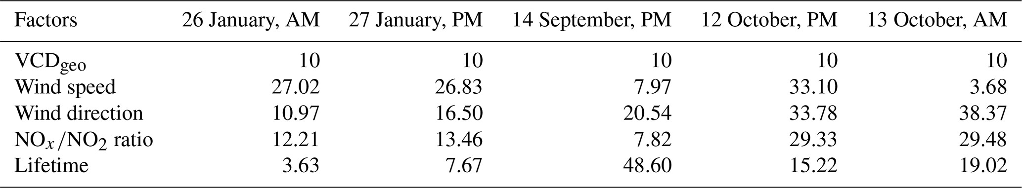
Table 3Error contributions (%) of multiple factors to the uncertainties in estimated during five circling journeys.
3.4 Uncertainty analysis of estimated emissions
We calculated the uncertainty of according to the error transfer formula of relative deviation based on the errors of measured NO2 VCD and simulated wind speed and direction, cL and cτ. The standard deviation (SD) of wind speed over a period of time can provide a bound for the related uncertainties of the emission estimate (Ibrahim et al., 2010). Therefore, we first computed the uncertainty of based on the SD of simulated wind speed after correction and the measurement error of NO2 VCD (about ±10 %, Ma et al., 2013a) for each journey. Then, we calculated the SD of cτ according to the first derivative of Eq. (4) and the SD of cL using a different NOx lifetime and the ratios of NOx and NO2 at sampling positions on the 6th Ring Rd of Beijing for each journey. Figure 11 shows the uncertainties of for five journeys, and the uncertainty range of is 2.2×1025 to 9.1×1025 molec. s−1 (20 %–52 %).
We also give the spatial variation in the NOx∕NO2 ratio and NOx lifetime at the entire route for the emission calculation during five journeys (Figs. S7 and S8) and estimate the error contribution of five factors, including NO2 VCD, wind speed, wind direction, the NOx∕NO2 ratio, and the NOx lifetime to the total uncertainty of (Table 3). In general, there are obvious seasonal and regional differences in the NOx∕NO2 ratio and NOx lifetime, and it is necessary to use specific ratios and lifetime values to estimate the for each journey. Specifically, the NOx∕NO2 ratio and NOx lifetime are larger in January than September and October, and they are larger at the southern part of the 6th Ring Rd than in other parts for most journeys. Among error contributions of the five factors, the impacts of wind speed and direction are the largest for most journeys except for 14 September. For 26 and 27 January, error contributions of wind speed to the uncertainty of are larger than the other four factors. For 14 September, uncertainty of is mainly caused by the errors of NOx lifetime and wind direction. For 12 and 13 October, error contributions of the NOx∕NO2 ratio are also remarkable. Thus, it is important to obtain the accurate wind vector profiles, NOx, NO2, and OH concentration data besides measured NO2 VCD to reduce the uncertainty of estimation using the CIM.
We also calculate the Leighton ratios, Lr, to assess impacts of VOCs on the NOx lifetime. The Lr during five journeys is 0.85, 0.80, 1.04, 1.19, and 1.33 on 26 and 27 January, 14 September, and 12 and 13 October, respectively. Results show that VOCs can affect the NOx lifetime, which leads to extra errors of for the three journeys in September and October, while the uncertainty in VOCs causes insignificant deviations in the NOx lifetime and estimation in January.
We carried out 19 city-circle-around car MAX-DOAS experiments on the 6th Ring Rd of Beijing in January, September, and October 2014. The VCD of NO2 was retrieved, and the temporal and spatial distributions were investigated. Then the NOx emission rates in urban Beijing were estimated using the measured NO2 VCD together with the refined wind fields, NO2-to-NOx ratios, and NO2 lifetimes simulated by the LAPS-WRF-CMAQ model system, and the results were compared to the emission rates from the MEIC 2012.
The NO2 VCD values averaged for each experimental journey in January were all larger than those in the other 2 months, mainly due to higher emissions in winter. The measured NO2 VCD was typically larger in the southern parts of the 6th Ring Road than in the northern parts because weak southerly wind resulted in the transport and accumulation of NO2 from southern areas in Hebei Province and strong northerly wind suppressed the transport of NO2 from the southern area. Such inhomogeneous distributions of tropospheric NO2 VCD bring a challenge for the validation of satellite products for Beijing as well as other megacities.
The journey-to-journey variations in estimated were large, even within the same month, mainly due to uncertainties in the calculation of wind speed, the ratio of NO2 and NOx concentration, and the decay rate of NOx from the emission sources to the measured positions under different meteorological conditions. The average values in the heating and non-heating periods are estimated to be and molec. s−1, respectively, with an uncertainty range of 20 %–52 %. The monthly emission rates in the area within the 6th Ring Rd of Beijing from MEIC 2012 are lower than the estimated , particularly in January. The differences between the and the monthly emission rates from MEIC 2012 can be attributed to the interannual differences in the emission inventory, the different timescales, and uncertainties of two kinds of inventories.
Our results show that car MAX-DOAS measurements can be used effectively for dynamic monitoring and updating of the NOx emissions in megacities such as Beijing. To accurately estimate the by car MAX-DOAS in Beijing and other similar megacities, appropriate meteorological conditions, such as small fluctuations of the wind field, relatively larger wind speed, and suitable wind direction, need to be selected to avoid the impact of extra transfers of large emission sources from surrounding areas. In addition to the NO2 VCD, simultaneous observations of wind speed, wind direction, and surface NO and NO2 concentrations are recommended to reduce the uncertainties of .
The NCEP-FNL reanalysis and ECMWF are publicly available at https://doi.org/10.5065/D6M043C6 (National Center for Atmospheric Research, 2020) and https://apps.ecmwf.int/datasets/data/interim-full-daily/levtype=sfc (European Centre for Medium-Range Weather Forecasts, 2019), respectively. The NO2 measurements and meteorological observations including wind speed and wind direction data are available at http://www.cnemc.cn/en and http://data.cma.cn/ (China National Environmental Monitoring Centre, 2020), respectively. The tropospheric NO2 VCD data derived from this study are available on request.
The supplement related to this article is available online at: https://doi.org/10.5194/acp-20-10757-2020-supplement.
JM and XC designed the research. JM, JJ, JG, MQ, QX, and PY contributed to the measurements, and JM performed the spectral analysis and retrieval. XC and JP designed the model experiment and performed the model simulations. XC, YL, JP, and XM contributed to the data processing and analyses. XC and JM analyzed the results and wrote the paper with inputs from all the authors.
The authors declare that they have no conflict of interest.
We are grateful to Tsinghua University for providing the emission inventory and the China National Environmental Monitoring Centre for providing surface NO2 observation data. The authors would like to thank the editor Robert McLaren and the anonymous reviewers for their constructive advice.
This work was supported jointly by the National Natural Science Foundation of China (grant nos. 91644223 and 91937302), the National Research Program for Key Issues in Air Pollution Control (grant no. DQGG0104), and the National Key Research and Development Program of China (grant no. 2018YFB1500901).
This paper was edited by Robert McLaren and reviewed by two anonymous referees.
Albers, S. C., McGinley, J. A., Birkenheuer, D., and Smart, J. R.: The local analysis and prediction system (LAPS): Analyses of clouds, precipitation, and temperature, Weather Forecast., 11, 273–287, 1996.
Brinksma, E. J., Pinardi, G., Volten, H., Braak, R., Richter, A., Schoenhardt, A., van Roozendael, M., Fayt, C., Hermans, C., Dirksen, R. J., Vlemmix, T., Berkhout, A. J. C., Swart, D. P. J., Oetjen, H., Wittrock, F., Wagner, T., Ibrahim, O. W., de Leeuw, G., Moerman, M., Curier, R. L., Celarier, E. A., Cede, A., Knap, W. H., Veefkind, J. P., Eskes, H. J., Allaart, M., Rothe, R., Piters, A. J. M., and Levelt, P. F.: The 2005 and 2006 DANDELIONS NO2 and aerosol intercomparison campaigns, J. Geophys. Res.-Atmos., 113, D16S46, https://doi.org/10.1029/2007JD008808, 2008.
Burrows, J. P., Richter, A., Dehn, A., Deters, B., Himmelmann, S., Voigt, S., and Orphal, J.: Atmospheric remote sensing reference data from GOME-2. temperature-dependent absorption cross-sections of O3 in the 231–794 nm range, J. Quant. Spectrosc. Ra., 61, 509–517, 1999.
Cao, C., Jiang, W., Wang, B., Fang, J., Lang, J., Tian, G., Jiang, J., and Zhu, T. F.: Inhalable microorganisms in Beijing's PM2.5 and PM10 pollutants during a severe smog event, Environ. Sci. Technol., 48, 1499–1507, https://doi.org/10.1021/es4048472, 2014.
Cheng, X., Sun, Z., Li, D., Xu, X., Jia, M., and Cheng, S.: Short-term aerosol radiative effects and their regional difference during heavy haze episodes in January 2013 in China, Atmos. Environ., 165, 248-263, https://doi.org/10.1016/j.atmosenv.2017.06.040, 2017.
China National Environmental Monitoring Centre: Real-time National Air Quality data, available at: http://www.cnemc.cn/en and http://data.cma.cn/, last access: September 2020.
Davis, Z. Y. W., Baray, S., McLinden, C. A., Khanbabakhani, A., Fujs, W., Csukat, C., Debosz, J., and McLaren, R.: Estimation of NOx and SO2 emissions from Sarnia, Ontario, using a mobile MAX-DOAS (Multi-AXis Differential Optical Absorption Spectroscopy) and a NOx analyzer, Atmos. Chem. Phys., 19, 13871–13889, https://doi.org/10.5194/acp-19-13871-2019, 2019.
Dennis, R., Byun, D., and Novak, J.: The next generation of integrated air quality modeling: EPA's Models-3, Atmos. Environ., 30, 1925–1938, 1996.
Dickerson, R. R., Stedman, D. H., and Delany, A. C.: Direct measurements of ozone and nitrogen dioxide photolysis rates in the troposphere, J. Geophys. Res., 87, 4933–4946, https://doi.org/10.1029/JC087iC07p04933, 1982.
European Centre for Medium-Range Weather Forecasts: ERA Interim data, available at: https://apps.ecmwf.int/datasets/data/interim-full-daily/levtype=sfc, last access: August 2019.
Fayt, C. and Van Roozendael, M.: WinDOAS 2.1 software user manual, IASB/BIRA Uccle, Belgium, 2011.
Greenblatt, G. D., Orlando, J. J., Burkholder, J. B., and Ravishankara, A. R.: Absorption measurements of oxygen between 330 and 1140 nm, J. Geophys. Res., 95, 18577–18582, https://doi.org/10.1029/JD095iD11p18577, 1990.
Hönninger, G. and Platt, U.: Observations of BrO and its vertical distribution during surface ozone depletion at Alert, Atmos. Environ., 36, 2481–2489, https://doi.org/10.1016/S1352-2310(02)00104-8, 2002.
Hönninger, G., von Friedeburg, C., and Platt, U.: Multi axis differential optical absorption spectroscopy (MAX-DOAS), Atmos. Chem. Phys., 4, 231–254, https://doi.org/10.5194/acp-4-231-2004, 2004.
Hao, J., Tian, H., and Lu, Y.: Emission inventories of NOx from commercial energy consumption in China, 1995–1998, Environ. Sci. Technol., 36, 552–560, 2002.
He, H., Wang, X. M., Wang, Y. S., Wang, Z. F., Liu, J. G., and Chen, Y. F.: Formation Mechanism and Control Strategies of Haze in China, Bull. Chin. Acad. Sci., 28, 344–352, 2013.
Hendrick, F., Müller, J.-F., Clémer, K., Wang, P., De Mazière, M., Fayt, C., Gielen, C., Hermans, C., Ma, J. Z., Pinardi, G., Stavrakou, T., Vlemmix, T., and Van Roozendael, M.: Four years of ground-based MAX-DOAS observations of HONO and NO2 in the Beijing area, Atmos. Chem. Phys., 14, 765–781, https://doi.org/10.5194/acp-14-765-2014, 2014.
Huang, R. J., Zhang, Y., Bozzetti, C., Ho, K. F., Cao, J. J., Han, Y., Daellenbach, K. R., Slowik, J. G., Platt, S. M., Canonaco, F., Zotter, P., Wolf, R., Pieber, S. M., Bruns, E. A., Crippa, M., Ciarelli, G., Piazzalunga, A., Schwikowski, M., Abbaszade, G., Schnelle-Kreis, J., Zimmermann, R., An, Z., Szidat, S., Baltensperger, U., El Haddad, I., and Prevot, A. S.: High secondary aerosol contribution to particulate pollution during haze events in China, Nature, 514, 218–222, https://doi.org/10.1038/nature13774, 2014.
Ibrahim, O., Shaiganfar, R., Sinreich, R., Stein, T., Platt, U., and Wagner, T.: Car MAX-DOAS measurements around entire cities: quantification of NOx emissions from the cities of Mannheim and Ludwigshafen (Germany), Atmos. Meas. Tech., 3, 709–721, https://doi.org/10.5194/amt-3-709-2010, 2010.
Irie, H., Kanaya, Y., Akimoto, H., Tanimoto, H., Wang, Z., Gleason, J. F., and Bucsela, E. J.: Validation of OMI tropospheric NO2 column data using MAX-DOAS measurements deep inside the North China Plain in June 2006: Mount Tai Experiment 2006, Atmos. Chem. Phys., 8, 6577–6586, https://doi.org/10.5194/acp-8-6577-2008, 2008.
Jaeglé, L., Steinberger, L., Martin, R. V., and Chance, K.: Global partitioning of NOx sources using satellite observations: relative roles of fossil fuel combustion, biomass burning and soil emissions, Roy. Soc. Chem., 130, 407–423, 2005.
Jin, J., Ma, J., Lin, W., Zhao, H., Shaiganfar, R., Beirle, S., and Wagner, T.: MAX-DOAS measurements and satellite validation of tropospheric NO2 and SO2 vertical column densities at a rural site of North China, Atmos. Environ., 133, 12–25, https://doi.org/10.1016/j.atmosenv.2016.03.031, 2016.
Johansson, M., Galle, B., Yu, T., Tang, L., Chen, D., Li, H., Li, J. X., and Zhang, Y.: Quantification of total emission of air pollutants from Beijing using mobile mini-DOAS, Atmos. Environ., 42, 6926–6933, https://doi.org/10.1016/j.atmosenv.2008.05.025, 2008.
Johansson, M., Rivera, C., de Foy, B., Lei, W., Song, J., Zhang, Y., Galle, B., and Molina, L.: Mobile mini-DOAS measurement of the outflow of NO2 and HCHO from Mexico City, Atmos. Chem. Phys., 9, 5647–5653, https://doi.org/10.5194/acp-9-5647-2009, 2009.
Konovalov, I. B., Beekmann, M., Richter, A., and Burrows, J. P.: Inverse modelling of the spatial distribution of NOx emissions on a continental scale using satellite data, Atmos. Chem. Phys., 6, 1747–1770, https://doi.org/10.5194/acp-6-1747-2006, 2006.
Kraus, S.: DOASIS, DOAS for Windows software [CD-ROM], in: Proceedings of the 1st International DOAS-Workshop, 13–14 September 2001, Heidelberg, Germany, 2001.
Li, M., Liu, H., Geng, G., Hong, C., Liu, F., Song, Y., Tong, D., Zheng, B., Cui, H., Man, H., Zhang, Q., and He, K.: Anthropogenic emission inventories in China: a review, Natl. Sci. Rev., 4, 834–866, https://doi.org/10.1093/nsr/nwx150, 2017.
Li, X., Brauers, T., Hofzumahaus, A., Lu, K., Li, Y. P., Shao, M., Wagner, T., and Wahner, A.: MAX-DOAS measurements of NO2, HCHO and CHOCHO at a rural site in Southern China, Atmos. Chem. Phys., 13, 2133–2151, https://doi.org/10.5194/acp-13-2133-2013, 2013.
Liao, L., Lou, S. J., Fu, Y., Chang, W. J., and Liao, H.: Radiative forcing of aerosols and its impact on surface air temperature on the synoptic scale in eastern China, Chin. J. Atmos. Sci., 39, 68–82, 2015.
Lin, J.-T., Liu, Z., Zhang, Q., Liu, H., Mao, J., and Zhuang, G.: Modeling uncertainties for tropospheric nitrogen dioxide columns affecting satellite-based inverse modeling of nitrogen oxides emissions, Atmos. Chem. Phys., 12, 12255–12275, https://doi.org/10.5194/acp-12-12255-2012, 2012.
Ma, J. and van Aardenne, J. A.: Impact of different emission inventories on simulated tropospheric ozone over China: a regional chemical transport model evaluation, Atmos. Chem. Phys., 4, 877–887, https://doi.org/10.5194/acp-4-877-2004, 2004.
Ma, J. Z., Wang, W., Chen, Y., Liu, H. J., Yan, P., Ding, G. A., Wang, M. L., Sun, J., and Lelieveld, J.: The IPAC-NC field campaign: a pollution and oxidization pool in the lower atmosphere over Huabei, China, Atmos. Chem. Phys., 12, 3883–3908, https://doi.org/10.5194/acp-12-3883-2012, 2012.
Ma, J. Z., Beirle, S., Jin, J. L., Shaiganfar, R., Yan, P., and Wagner, T.: Tropospheric NO2 vertical column densities over Beijing: results of the first three years of ground-based MAX-DOAS measurements (2008–2011) and satellite validation, Atmos. Chem. Phys., 13, 1547–1567, https://doi.org/10.5194/acp-13-1547-2013, 2013a.
Ma, J. Z., Wang, W., Liu, H., Chen, Y., Xu, X., and Lelieveld, J.: Pollution plumes observed by aircraft over North China during the IPAC-NC field campaign, Chinese Sci. Bull., 58, 4329–4336, https://doi.org/10.1007/s11434-013-5978-9, 2013b.
Martin, R. V.: An improved retrieval of tropospheric nitrogen dioxide from GOME, J. Geophys. Res., 107, ACH 9-1–ACH 9-21, https://doi.org/10.1029/2001jd001027, 2002.
McGinley, J. A., Albers, S., and Stamus, P.: Validation of a composite convective index as defined by a real-time local analysis system, Weather Forecast., 6, 337–356, 1991.
Meng, K., Xu, X., Cheng, X., Xu, X., Qu, X., Zhu, W., Ma, C., Yang, Y., and Zhao, Y.: Spatio-temporal variations in SO2 and NO2 emissions caused by heating over the Beijing-Tianjin-Hebei Region constrained by an adaptive nudging method with OMI data, Sci. Total Environ., 642, 543–552, https://doi.org/10.1016/j.scitotenv.2018.06.021, 2018.
Michalakes, J., Dudhia, J., Gill, D., Henderson, T., Klemp, J., Skamarock, W., and Wang, W.: The weather research and forecast model: software architecture and performance, the 11th ECMWFWorkshop on the Use of High Performance Computing In Meteorology, World Scientific Publishing Co Pte Ltd, Singapore, George Mozdzynski, 2004.
National Center for Atmospheric Research: NCEP FNL Operational Model Global Tropospheric Analyses data, available at: https://doi.org/10.5065/D6M043C6, last access: September 2020.
Otte, T. L. and Pleim, J. E.: The Meteorology-Chemistry Interface Processor (MCIP) for the CMAQ modeling system: updates through MCIPv3.4.1, Geosci. Model Dev., 3, 243–256, https://doi.org/10.5194/gmd-3-243-2010, 2010.
Platt, U.: Differential optical absorption spectroscopy (DOAS), in: Air Monitoring by Spectroscopic Techniques, edited by: Sigrist, M. W., Chemical Analysis Series, Vol. 127, John Wiley, New York, 27–84, 1994.
Platt, U. and Stutz, J.: Differential Optical Absorption Spectroscopy Principles and Applications, Physics of Earth and Space Environments, Springer, Heidelberg, 2008.
Shaiganfar, R., Beirle, S., Sharma, M., Chauhan, A., Singh, R. P., and Wagner, T.: Estimation of NOx emissions from Delhi using Car MAX-DOAS observations and comparison with OMI satellite data, Atmos. Chem. Phys., 11, 10871–10887, https://doi.org/10.5194/acp-11-10871-2011, 2011.
Shaiganfar, R., Beirle, S., Denier van der Gon, H., Jonkers, S., Kuenen, J., Petetin, H., Zhang, Q., Beekmann, M., and Wagner, T.: Estimation of the Paris NOx emissions from mobile MAX-DOAS observations and CHIMERE model simulations during the MEGAPOLI campaign using the closed integral method, Atmos. Chem. Phys., 17, 7853–7890, https://doi.org/10.5194/acp-17-7853-2017, 2017.
Streets, D. G., Canty, T., Carmichael, G. R., de Foy, B., Dickerson, R. R., Duncan, B. N., Edwards, D. P., Haynes, J. A., Henze, D. K., Houyoux, M. R., Jacob, D. J., Krotkov, N. A., Lamsal, L. N., Liu, Y., Lu, Z., Martin, R. V., Pfister, G. G., Pinder, R. W., Salawitch, R. J., and Wecht, K. J.: Emissions estimation from satellite retrievals: A review of current capability, Atmos. Environ., 77, 1011–1042, https://doi.org/10.1016/j.atmosenv.2013.05.051, 2013.
Tan, T., Hu, M., Li, M., Guo, Q., Wu, Y., Fang, X., Gu, F., Wang, Y., and Wu, Z.: New insight into PM2.5 pollution patterns in Beijing based on one-year measurement of chemical compositions, Sci. Total Environ., 621, 734–743, https://doi.org/10.1016/j.scitotenv.2017.11.208, 2018.
UNC: SMOKE v3.6 user's manual, The institute for the Environment, Chapel Hill, 2014.
Valin, L. C., Russell, A. R., and Cohen, R. C.: Variations of OH radical in an urban plume inferred from NO2 column measurements, Geophys. Res. Lett., 40, 1856–1860, https://doi.org/10.1002/grl.50267, 2013.
Vandaele, A. C., Hermans, C., Simon, P. C., Carleer, M., Colin, R., Fally, S., Mérienne, M. F., Jenouvrier, A., and Coquart, B.: Measurements of the NO2 absorption cross-section from 42 000 cm−1 to 10 000 cm−1 (238–1000 nm) at 220 K and 294 K, J. Quant. Spectrosc. Ra., 59, 171–184, 1998.
Vlemmix, T., Piters, A. J. M., Stammes, P., Wang, P., and Levelt, P. F.: Retrieval of tropospheric NO2 using the MAX-DOAS method combined with relative intensity measurements for aerosol correction, Atmos. Meas. Tech., 3, 1287–1305, https://doi.org/10.5194/amt-3-1287-2010, 2010.
Wagner, T., Dix, B., Friedeburg, C. v., Frieß, U., Sanghavi, S., Sinreich, R., and Platt, U.: MAX-DOAS O4 measurements: A new technique to derive information on atmospheric aerosols – Principles and information content, J. Geophys. Res., 109, D22205, https://doi.org/10.1029/2004jd004904, 2004.
Wagner, T., Ibrahim, O., Shaiganfar, R., and Platt, U.: Mobile MAX-DOAS observations of tropospheric trace gases, Atmos. Meas. Tech., 3, 129–140, https://doi.org/10.5194/amt-3-129-2010, 2010a.
Wagner, T., Ibrahim, O., Shaiganfar, R., and Platt, U.: Mobile MAX-DOAS observations of tropospheric trace gases, Atmos. Meas. Tech., 3, 129–140, https://doi.org/10.5194/amt-3-129-2010, 2010b.
Wagner, T., Beirle, S., Brauers, T., Deutschmann, T., Frieß, U., Hak, C., Halla, J. D., Heue, K. P., Junkermann, W., Li, X., Platt, U., and Pundt-Gruber, I.: Inversion of tropospheric profiles of aerosol extinction and HCHO and NO2 mixing ratios from MAX-DOAS observations in Milano during the summer of 2003 and comparison with independent data sets, Atmos. Meas. Tech., 4, 2685–2715, https://doi.org/10.5194/amt-4-2685-2011, 2011.
Wang, S., Zhou, B., Wang, Z., Yang, S., Hao, N., Valks, P., Trautmann, T., and Chen, L.: Remote sensing of NO2 emission from the central urban area of Shanghai (China) using the mobile DOAS technique, J. Geophys. Res.-Atmos., 117, D13305, https://doi.org/10.1029/2011jd016983, 2012.
Wang, Y., McElroy, M. B., Martin, R. V., Streets, D. G., Zhang, Q., and Fu, T.-M.: Seasonal variability of NOx emissions over east China constrained by satellite observations: Implications for combustion and microbial sources, J. Geophys. Res., 112, D06301, https://doi.org/10.1029/2006jd007538, 2007.
Wittrock, F., Oetjen, H., Richter, A., Fietkau, S., Medeke, T., Rozanov, A., and Burrows, J. P.: MAX-DOAS measurements of atmospheric trace gases in Ny-Ålesund – Radiative transfer studies and their application, Atmos. Chem. Phys., 4, 955–966, https://doi.org/10.5194/acp-4-955-2004, 2004.
Wu, F., Xie, P., Li, A., Mou, F., Chen, H., Zhu, Y., Zhu, T., Liu, J., and Liu, W.: Investigations of temporal and spatial distribution of precursors SO2 and NO2 vertical columns in the North China Plain using mobile DOAS, Atmos. Chem. Phys., 18, 1535–1554, https://doi.org/10.5194/acp-18-1535-2018, 2018.
Zhang, Q., Streets, D. G., He, K., Wang, Y., Richter, A., Burrows, J. P., Uno, I., Jang, C. J., Chen, D., Yao, Z., and Lei, Y.: NOx emission trends for China, 1995–2004: The view from the ground and the view from space, J. Geophys. Res., 112, D22306, https://doi.org/10.1029/2007jd008684, 2007.
Zhang, Q., Streets, D. G., Carmichael, G. R., He, K. B., Huo, H., Kannari, A., Klimont, Z., Park, I. S., Reddy, S., Fu, J. S., Chen, D., Duan, L., Lei, Y., Wang, L. T., and Yao, Z. L.: Asian emissions in 2006 for the NASA INTEX-B mission, Atmos. Chem. Phys., 9, 5131–5153, https://doi.org/10.5194/acp-9-5131-2009, 2009.
Zhang, Q., Geng, G., Wang, S., Richter, A., and He, K.: Satellite remote sensing of changes in NOx emissions over China during 1996–2010, Chinese Science Bulletin, 57, 2857–2864, https://doi.org/10.1007/s11434-012-5015-4, 2012.
Zhang, X. Y., Sun, J. Y., Wang, Y. Q., Li, W. J., Zhang, Q., Wang, W. G., Quan, J. N., Cao, G. L., Wang, J. Z., Yang, Y. Q., and Zhang, Y. M.: Factors contributing to haze and fog in China, Chinese Sci. Bull., 58, 1178–1187, 2013.
Zhao, B., Wang, P., Ma, J. Z., Zhu, S., Pozzer, A., and Li, W.: A high-resolution emission inventory of primary pollutants for the Huabei region, China, Atmos. Chem. Phys., 12, 481–501, https://doi.org/10.5194/acp-12-481-2012, 2012.
Zyrichidou, I., Koukouli, M. E., Balis, D., Markakis, K., Poupkou, A., Katragkou, E., Kioutsioukis, I., Melas, D., Boersma, K. F., and van Roozendael, M.: Identification of surface NOx emission sources on a regional scale using OMI NO2, Atmos. Environ., 101, 82–93, https://doi.org/10.1016/j.atmosenv.2014.11.023, 2015.