Sensitivity of GPS tropospheric estimates to mesoscale convective systems in West Africa

This study analyzes the characteristics of GPS tropospheric estimates (zenith wet delays – ZWDs, gradients, and post-fit phase residuals) during the passage of mesoscale convective systems (MCSs) and evaluates their sensitivity to the research-level GPS data processing strategy implemented. Here, we focus on MCS events observed during the monsoon season of West Africa. This region is particularly well suited for the study of these events due to the high frequency of MCS occurrences in the contrasting climatic environments between the Guinean coast and the Sahel. This contrast is well sampled with data generated by six African Monsoon Multidisciplinary Analysis (AMMA) GPS stations. Tropospheric estimates for a 3-year period (2006–2008), processed with both the GAMIT and GIPSY-OASIS software packages, were analyzed and intercompared. First, the case of a MCS that passed over Niamey, Niger, on 11 August 2006 demonstrates a strong impact of the MCS on GPS estimates and post-fit residuals when the GPS signals propagate through the convective cells as detected on reflectivity maps from the MIT C-band Doppler radar. The estimates are also capable of detecting changes in the structure and dynamics of the MCS. However, the sensitivity is different depending on the tropospheric modeling approach adopted in the software. With GIPSY-OASIS, the high temporal sampling (5 min) of ZWDs and gradients is well suited for detecting the small-scale, short-lived, convective cells, while the post-fit residuals remain quite small. With GAMIT, the lower temporal sampling of the estimated parameters (hourly for ZWDs and daily for gradients) is not sufficient to capture the rapid delay variations associated with the passage of the MCS, but the post-fit phase residuals clearly reflect the presence of a strong refractivity anomaly. The results are generalized with a composite analysis of 414 MCS events observed over the 3-year period at the six GPS stations with the GIPSY-OASIS estimates. A systematic peak is found in the ZWDs coincident with the cold pool crossing time associated with the MCSs. The tropospheric gradients reflect the path of the MCS propagation (generally from east to west). This study concludes that ZWDs, gradients, and post-fit phase residuals provide relevant and complementary information on MCSs passing over or in the vicinity of a GPS station.

1 Introduction

The American Meteorological Society (2015) defines a mesoscale convective system (MCS) as “a cloud system that occurs in connection with an ensemble of thunderstorms and produces a contiguous precipitation area on the order of 100 km or more in horizontal scale in at least one direction. A MCS exhibits deep, moist convective overturning contiguous with or embedded within a mesoscale vertical circulation that is at least partially driven by the convective overturning”. Figure 1 displays a typical nighttime example of the convective activity over West Africa during the monsoon season, with two active clusters of MCS on the eastern and western borders of Nigeria, and more scattered dissipating MCSs over Guinea. Small isolated developing MCSs can also be seen in northern Ghana and over the Senegal–Mauritania border. The MCS's internal structure typically comprises convective and stratiform regions as described by Zipser (1977), Houze et al. (1990), and Houze (1989, 1997, 2004). However, numerous questions related to MCSs remain poorly answered, such as the mechanisms behind their life cycle (their initialization, propagation, and decay; e.g., Laing et al., 2008), and how these mechanisms involve interactions between physical processes (e.g., surface and boundary layer processes – Taylor et al., 2017; Rochetin et al., 2017) and atmospheric circulations (e.g., African easterly waves – Fink et al., 2006; Rickenbach et al., 2009; Beucher et al., 2014).

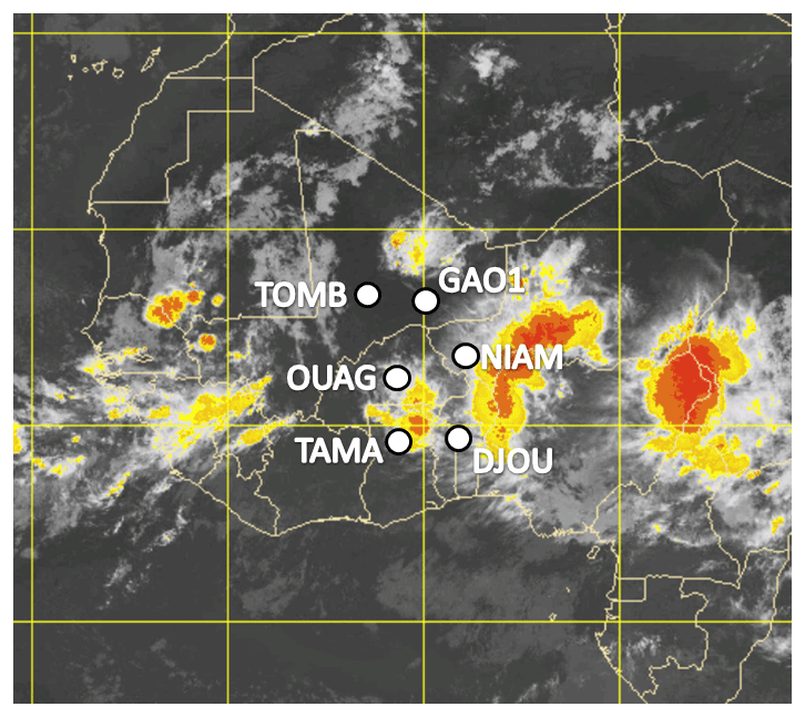
Figure 1 Meteosat-8 infrared image of West Africa on 10 August 2006 at 23:00 UTC. Brightness temperatures range between 225 K (yellow) and 195 K (red). The position of the six AMMA GPS stations are shown as white dots: TOMB (Timbuktu, Mali), GAO1 (Gao, Mali), OUAG (Ouagadougou, Burkina Faso), NIAM (Niamey, Niger), TAMA (Tamale, Ghana), and DJOU (Djougou, Benin). Meteosat-8 infrared background: © 2019 EUMETSAT.

Deep convection, MCSs, and rainfall are strongly linked to atmospheric water vapor (e.g., Bretherton et al., 2004; Schiro et al., 2016; Sherwood et al., 2010). This is why GPS integrated water vapor (IWV) data have been used for studies in various tropical climates such as the Indian monsoon (Jade et al., 2005; Jade and Vijayan, 2008), the South and North American monsoon (Gutzler et al., 2004; Means, 2013; Adams et al., 2011, 2014; Serra et al., 2016), and the West African monsoon (WAM) (Couvreux et al., 2012; Barthe et al., 2010). Here, we focus on MCSs occurring during the WAM, which has been the subject of intense investigations in recent years in the framework of the African Monsoon Multidisciplinary Analysis (AMMA) program (Redelsperger et al., 2006; Lafore et al., 2011). Indeed, MCSs are a key component of the WAM, as they produce 90 % of the annual rainfall in West Africa (D'Amato and Lebel, 1998). Within the AMMA's framework, six GPS stations (Fig. 1) were operated between 2005 and 2010 to sample IWV along the climatic gradient from the arid Saharo–Sahelian climate in Mali to the moist Sudano–Guinean climate in Benin (Bock et al., 2008). The AMMA GPS data have proved to be valuable for understanding the water cycle of this region including WAM atmospheric processes (Janicot et al., 2008; Lafore et al., 2011), land water storage changes (Hinderer et al., 2009), water budgets (Meynadier et al., 2010a, b), or hydrological loading deformation induced by the WAM (Nahmani et al., 2012).

Links between atmospheric water vapor and convective precipitation occur on various temporal scales down to less than a few hours. Notably, GPS data have revealed that a sharp IWV increase is often observed with the passage of MCSs (Barthe et al., 2010; Schiro et al., 2016; Taylor et al., 2017). In this study, we focus on this “small” scale (a few hours or less). More precisely, we address the question of the accuracy of AMMA GPS observations and the informational content of tropospheric delay estimates during the passage of MCSs over West Africa, comparing the two main research-level GPS data processing approaches: network processing, in which differentiated or undifferentiated observations from several stations are processed simultaneously, and precise point positioning (PPP), in which each station is processed independently but requires precise satellite orbits and clocks as calculated by the International GNSS Service (IGS) or one of its analysis centers (http://www.igs.org, last access: 25 July 2019). In both approaches, many processing options can be used, depending on the functionality of the software, such as least squares adjustment or Kalman filter, the choice of the elevation cutoff angle, the modeling of the troposphere, the rejection procedure of the erroneous observations (screening), among others. In this paper we compare the GPS Analysis at Massachusetts Institute of Technology (GAMIT) software (Herring et al., 2015) and the GNSS Inferred Positioning System and Orbit Analysis Simulation (GIPSY-OASIS) software from the NASA Jet Propulsion Laboratory (JPL)/Caltech (https://gipsy-oasis.jpl.nasa.gov/, last access: 25 July 2019). The first performs a least squares adjustment on a regional network with one zenith tropospheric delay (ZTD) estimated every hour, whereas the second uses a Kalman filter to process the data in PPP mode with one ZTD estimated every 5 min. Both software packages implement tropospheric delay models that also include gradient parameters. Gradient parameters allow for the representation of the effect of first-order azimuthal asymmetry in the atmospheric refractive index (MacMillan, 1995; MacMillan and Ma, 1997; Chen and Herring, 1997).The spatial scale over which the GPS measurements are sensitive to atmospheric refractivity gradients is about 50 km.

Section 2 discusses the processing options available in both software packages and the expected impact on the tropospheric delay estimates. Results are presented and discussed for the AMMA GPS stations over a continuous period of 3 years (2006 to 2008 – the most complete period for the six stations). The climatic context of West Africa lends itself particularly well to this methodological study with marked dry and wet seasons. Section 3 presents the case study of an organized cluster of MCSs passing over Niamey, Niger, on 11 August 2006 (Fig. 1). The case study illustrates the main characteristics of the MCS events captured by GPS tropospheric estimates according to the tropospheric modeling used during the data processing. Section 4 provides at statistical characterization of MCSs using GPS tropospheric delay estimates from 414 events observed by the six AMMA stations between 2006 and 2008. Section 5 concludes the study.

2 GPS data processing and methods

The six AMMA GPS stations used here meet the quality standards of the IGS (Dow et al., 2009) and are also equipped with meteorological sensors (Vaisala, PTU200). Their Receiver-Independent Exchange (RINEX) files are freely available on IGS servers (see the data availability section of this paper).

2.1 GPS data analysis with GAMIT

The RINEX data from the six AMMA GPS stations are processed from 1 January 2006 to 31 December 2008 within a regional network of around 25 IGS stations using the GAMIT scientific software (Herring et al., 2015) release 10.6. The settings of the GPS data processing are designed to meet the recommendations of the International Earth Rotation Service (IERS) conventions (Petit and Luzum, 2010) and correspond to an update of those used by Bock et al. (2008). The IGS final orbits are held fixed. A priori station positions expressed in ITRF2014 (Altamimi et al., 2016) are constrained with 10 and 30 cm a priori standard deviations for the horizontal and vertical components, respectively. GPS phase observations are corrected by applying absolute antenna phase calibration models (Schmid et al., 2007) and are weighted using the elevation-dependent variance function ${\mathit{\sigma }}^{\mathrm{2}}=a^{\mathrm{2}}+b^{\mathrm{2}}/{\sin }^{\mathrm{2}}\left(e\right)$, where e is the elevation angle and a and b are determined by a least squares of the post-fit residuals in an iterative procedure. The integer ambiguities are determined using wade-lane and narrow-lane combinations (Dong and Bock, 1989). The elevation cutoff angle is fixed to 7^∘. Ocean tide loading effects are corrected using the FES2004 model (Lyard et al., 2006). Atmospheric loading and non-tidal ocean loading can be neglected at AMMA GPS stations (Nahmani et al., 2012). This approximation introduces an uncertainty at a submillimetric level on zenith wet delay (ZWD) estimates at AMMA GPS stations (Nahmani, 2012). Concerning the propagation delays, the ionosphere-free phase combinations are corrected for second- and third-order ionospheric refraction terms (Hernandez-Pajares et al., 2007; Petrie et al., 2010). For tropospheric modeling, we use the VMF1 mapping functions and a priori hydrostatic delays derived from the European Centre for Medium-Range Weather Forecasts (ECMWF) model (Boehm et al., 2006b). The ZWDs and total tropospheric horizontal gradients are estimated with sampling intervals of 1 and 24 h, respectively. During the least squares estimation, the ZWD is represented by a piecewise linear function with hourly nodes modeled as a random walk, i.e., $\mathrm{ZWD}(t+\mathrm{\Delta }t)=\mathrm{ZWD}\left(t\right)+\mathit{\epsilon }\left(t\right)$. The variance of the white noise ε(t) is parameterized as ${\mathit{\sigma }}_{\mathit{\epsilon }}^{\mathrm{2}}=q_{\mathrm{rw}}^{\mathrm{2}}\cdot \mathrm{\Delta }t$, where Δt=1 h, and the parameter q_rw is fixed to the recommended value of 20 mm h${}^{-\mathrm{1}/\mathrm{2}}$ (Herring et al., 2015). To avoid edge effects on the ZWD estimates, we use a sliding window technique. We process GPS data in two 24 h sessions, the first starting at 00:00 UTC and the second at 12:00 UTC, from which the central 12 h output estimates are extracted as the final solutions. At the end of each session processing, the estimated tropospheric delays, tropospheric gradients, and the GPS one-way phase residuals (Herring et al., 2015) are saved for each AMMA station (Table 1).

Table 1 GPS data processing details with the GAMIT and GIPSY-OASIS software packages.

The processing of GPS data with the GAMIT software has some limitations: the ZWD temporal sampling interval of 1 h and the gradient temporal sampling interval of 24 h are too coarse to document the rapid meteorological extreme events like the passage of MCSs. Indeed, in such situations, rapid variations in the ZWD and strong anisotropy in the refractivity field are observed (Bock et al., 2008). As a consequence of the severe mis-modeling of the propagation delays, the estimated ZWD and gradient parameters are likely biased. Inspection of the post-fit phase residuals will help identify the severity of the mis-modeling. This mis-modeling can be partly overcome via the use of a PPP Kalman-filter-based software to increase the sampling interval of ZWD and gradient estimates. The PPP approach also has the advantage of eliminating the propagation of errors induced by the mis-modeling between stations.

2.2 GPS data analysis with GIPSY-OASIS in PPP mode

The GIPSY-OASIS II v 6.3 software is based on a Kalman-filter estimator (Zumberge et al., 1997). We used it in PPP mode to reprocess the AMMA GPS data with a parameterization that is as similar as possible to the settings used with the GAMIT software described in Sect. 2.1. Table 1 summarizes the different strategies used to process the GPS data. Compared with GAMIT, a major difference with GIPSY-OASIS II is the sampling interval of the estimated parameters (ZWDs, tropospheric gradients, and receiver clocks) of 5 min, which is achievable thanks to the Kalman-filter technique in which the parameters are updated at each time step. A minor drawback is that the GPS phase observations are thus reduced to a 5 min interval, i.e., this estimation procedure uses 10 times fewer observations than the GAMIT processing. A few other minor differences are also found in the observation weighting function, which is modeled as ${\mathit{\sigma }}^{\mathrm{2}}=a^{\mathrm{2}}/{\sin }^{\mathrm{2}}\left(e\right)$ with a fixed to 10 mm, and in the phase ambiguities resolution methods (GIPSY-OASIS II v6.3 uses the “ambigon” algorithm of Bertiger et al., 2010). To avoid edge effects, we followed the standard procedure used at JPL. The GPS data are analyzed in a 30 h window centered on each day, from which the 00:00–24:00 UTC parameters are extracted. This is also consistent with the JPL satellite orbit and clock products that are used instead of the IGS products. Regarding tropospheric modeling, the ZWD and tropospheric gradient parameters are modeled as random walk processes with a 5 min time resolution. However, the question then arises as to the choice of the parameterization of the random walk. The recommendations in the GIPSY-OASIS II documentation are mainly based on the results of Bar-Sever et al. (1998) and updated by Selle and Desai (2016). They suggest that the parameter of the ZWD random walk should be set to at least 8.4 mm h${}^{-\mathrm{1}/\mathrm{2}}$ when using ${\mathit{\sigma }}^{\mathrm{2}}=a^{\mathrm{2}}/{\sin }^{\mathrm{2}}\left(e\right)$ as the weighting function for the GPS observations (as opposed to 20 mm h${}^{-\mathrm{1}/\mathrm{2}}$ in the GAMIT software). However, Jarlemark et al. (1998) noticed that using a random walk parameter tighter than the real atmospheric variability introduces errors in the ZWD estimates. As this study is focused on MCSs which correspond to severe weather events, we can expect a very high variability in the tropospheric parameters; hence, it seems more reasonable to set the random walk parameter to the looser recommended value in both software packages rather than to the tighter. As for the temporal evolution model of tropospheric gradients, it is common to use a random walk for which the parameter is 10 times smaller than that of the ZWD (Bar-Sever et al., 1998). Thus, we keep the GAMIT-recommended random walk parameter of ZWD at 20 mm h${}^{-\mathrm{1}/\mathrm{2}}$ and set the random walk parameter of the tropospheric gradients to 2 mm h${}^{-\mathrm{1}/\mathrm{2}}$.

2.3 Comparison and quality of the GPS solutions from the GAMIT and GIPSY-OASIS software packages

2.3.1 ZWD and gradients

The time series of ZWDs retrieved by the GAMIT software at Timbuktu, Niamey, and Djougou, between 2006 and 2008, display a well-defined annual cycle (Fig. 2). The dry seasons are characterized by ZWDs of less than 100 mm (ca. between December and March), whereas the wet seasons, also referred to as the monsoon seasons, between June and September (hereafter referred to as JJAS), are characterized by frequent rain events and ZWD values higher than 200 mm (Bock et al., 2008). The duration of the monsoon season shrinks as one goes from the wetter climate in the south to the more arid climate in the north.

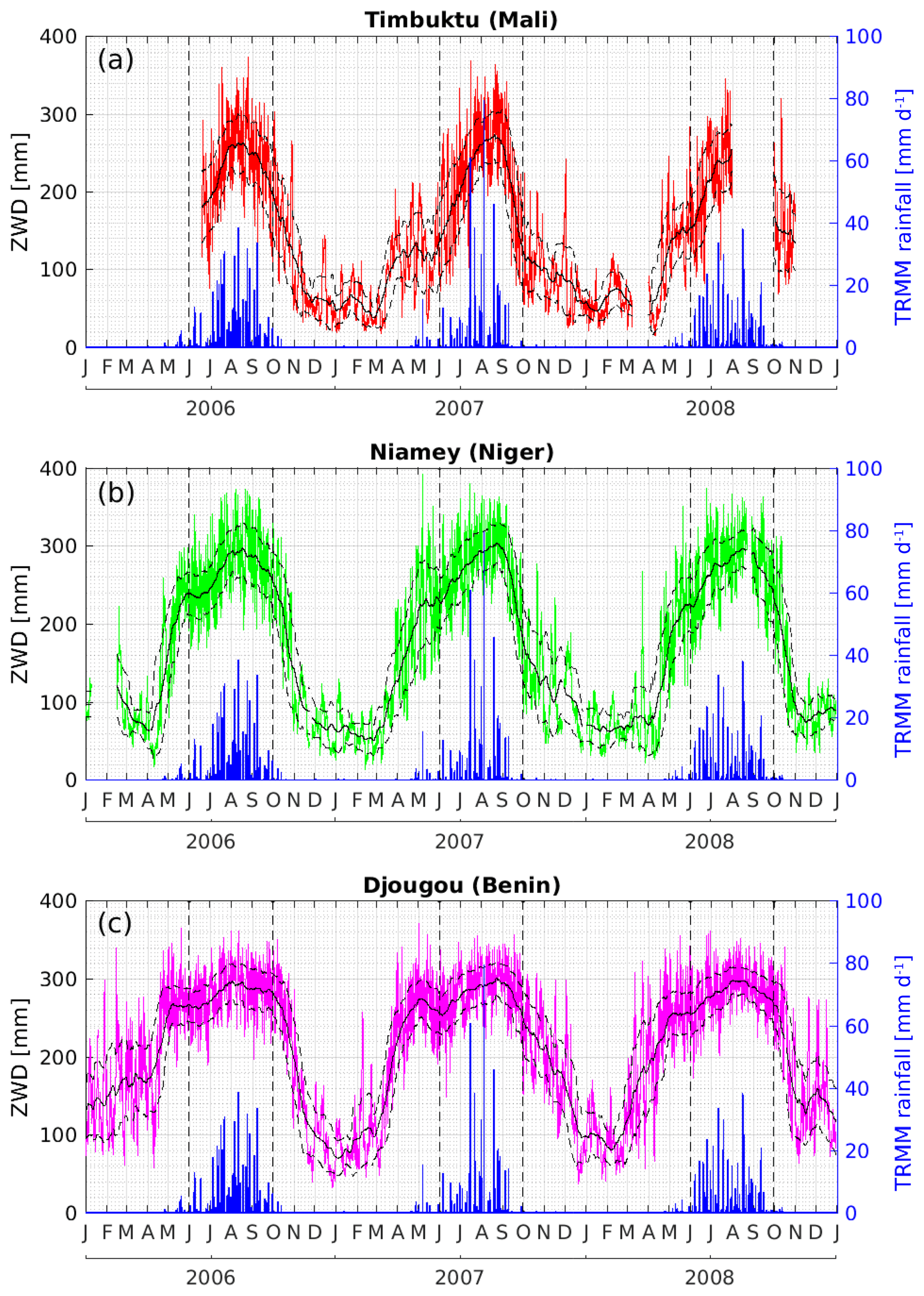
Figure 2 Time series of GPS-derived ZWD values retrieved with the GAMIT software and rainfall retrieved from the TRMM Multisatellite Precipitation Analysis (Huffman et al., 2007) at (a) Timbuktu, (b) Niamey, and (c) Djougou. The thin black solid and dashed lines show 30 d moving averages and standard deviations, respectively. The dashed black vertical lines delimit the period between June and September corresponding to the main rainy season.

Table 2 presents the statistics of the differences in the ZWD estimates (ΔZWD) obtained with both software packages during the monsoon season. The average differences of the ZWD values range from −0.45 mm at Gao to 0.96 mm at Djougou. They are small but statistically significant at all stations (95 % confidence level) and might be explained by minor differences persisting between the two GPS data processing methods (differences in orbits, tropospheric modeling, weighting of observations, and the potential rejection of some data). Standard deviations of ΔZWD range from 3.69 mm at Tamale to 4.30 mm at Gao. To understand the origin of these differences, we carried out a further statistical analysis of the tropospheric estimates presented in Fig. 3 for ZWDs and in Fig. 4 for gradients at Niamey. Figure 3a shows that the time series of ΔZWD exhibits a greater dispersion during the wet season than during the dry season as expected from larger (smaller) biases and mis-modeling of tropospheric refractivity with GAMIT during the wet (dry) season. To better characterize the timescales of atmospheric variability we computed sub-daily and sub-hourly variability estimates. To quantify the sub-daily (i.e., diurnal) variability, we subtracted a 1 d moving average from the hourly time series and then computed daily standard deviations. The sub-hourly variability was quantified in a similar way: by subtracting the hourly time series from the 5 min time series. Figure 3b and c show that the sub-daily and sub-hourly variability in ZWD estimated with GIPSY-OASIS dramatically increases during the wet season. The GAMIT solution presents very similar behavior for the sub-daily variability (not shown), but careful inspection of the 30 d smoothed time series in Fig. 3b shows that the GAMIT solution exhibits slightly larger sub-daily variability than GIPSY-OASIS solution during the wet season. This can be explained by random ZWD biases induced by mis-modeling. Indeed, the tropospheric modeling used in the GAMIT software does not take the sub-daily variations of the gradients into account nor does it account for the sub-hourly variations of ZWD. Therefore, the effect is more pronounced during the wet season because of higher tropospheric variability in these parameters as shown in Figs. 3c and 4 (and further analyzed in a case study in Sect. 3).

Table 2 Statistics of ZWD differences from GAMIT and GIPSY-OASIS processing solutions (GAMIT minus GIPSY-OASIS) for June to September, 2006–2008. The GIPSY-OASIS ZWD estimates were averaged over 1 h intervals beforehand. The last column gives the p value of a t test for the difference of the means. Values smaller than $\mathrm{1}\times {\mathrm{10}}^{-\mathrm{7}}$ are replaced with zero.

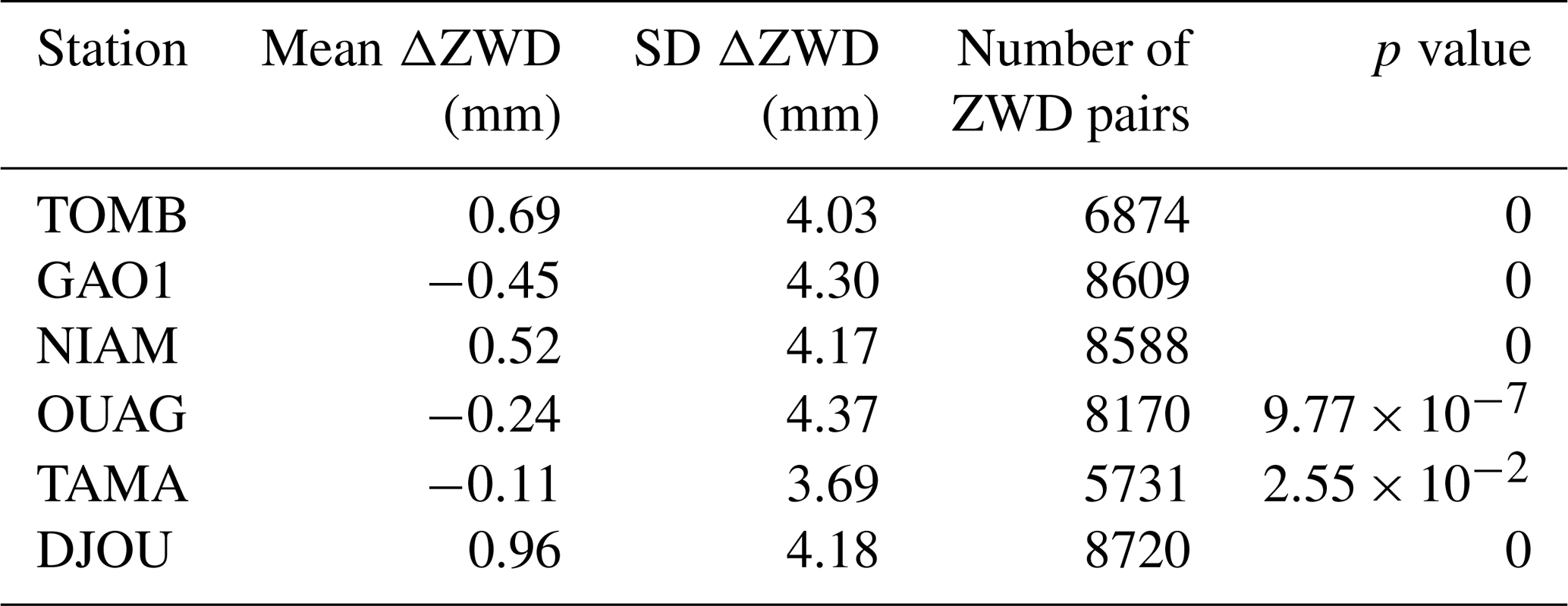
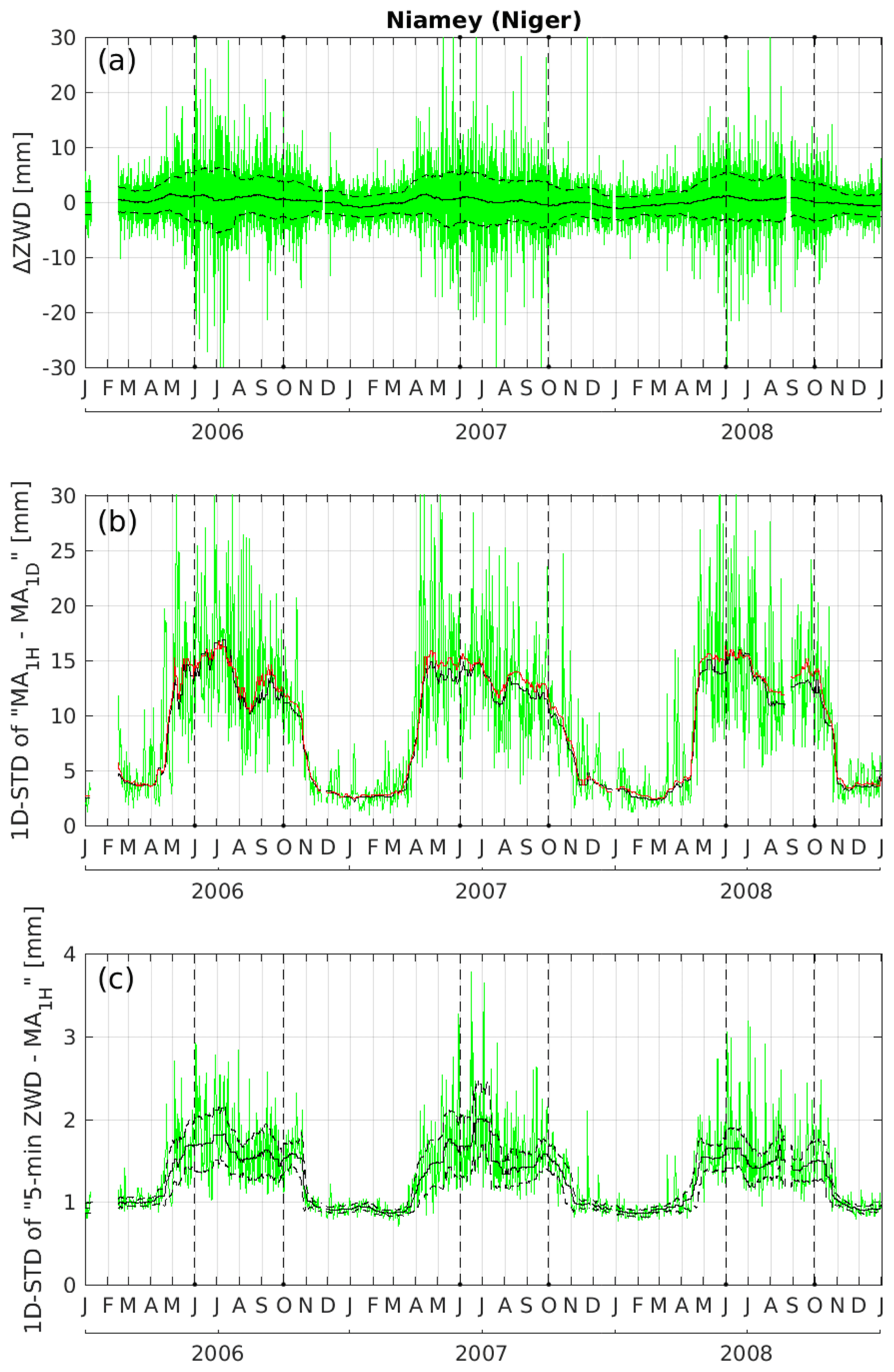
Figure 3 Analysis of the variability of GPS-derived ZWD at Niamey. (a) Difference between GAMIT and GIPSY-OASIS hourly ZWD estimates. (b) Sub-daily ZWD variability from GIPSY-OASIS (the daily standard deviation of the hourly minus the daily mean ZWD series is shown in green). (c) Sub-hourly ZWD variability from GIPSY-OASIS (the daily standard deviation of the 5 min minus the hourly ZWD series is shown in green). The thin black solid lines in panels (a), (b), and (c) show the 30 d moving medians. The red line in panel (b) shows a 30 d moving median of the sub-daily variability computed from the ZWD estimates retrieved by GAMIT. The thin black dashed lines in panels (a) and (c) show the median absolute deviations around the medians. Dashed black vertical lines indicate the JJAS period of each year.

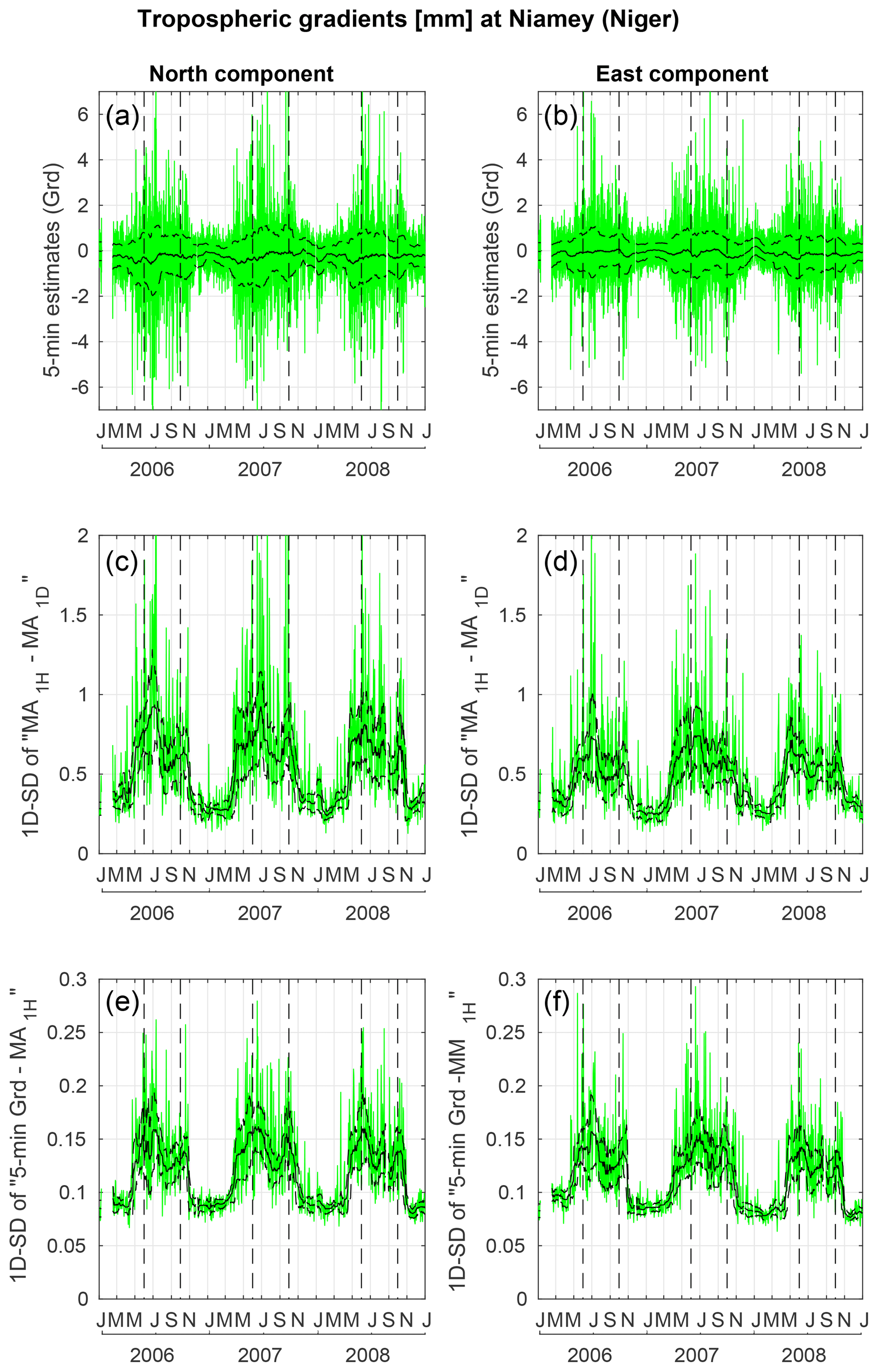
Figure 4 (a) North and (b) east components of the 5 min tropospheric gradients retrieved with the GIPSY-OASIS software at Niamey between 2006 and 2008, with the 30 d moving averages shown as solid black lines, and the 30 d moving standard deviations around the means shown as dashed black lines. (c, d) Sub-daily variability of north and east gradients (similar to Fig. 3b). (e, f) Sub-hourly variability of north and east gradients (similar to Fig. 3c). In panels (c)–(f), the solid black lines show 30 d moving medians, and the dashed black lines show moving median absolute deviations around the medians. The dashed black vertical lines indicate the JJAS period of each year.

Tropospheric gradients show a strong seasonality in phase with the WAM (Fig. 4a, b). The daily averages of gradients are in good agreement between the two software packages (not shown) with a mean difference smaller than a tenth of a millimeter and a standard deviation smaller than 0.22 mm due to biases induced by the un-modeled sub-daily variability. The sub-daily variations of the gradients estimated with GIPSY-OASIS can be quite large (up to 2 mm), with an average standard deviation of around 0.6 mm in both components, during the wet season (Fig. 4c, d). In contrast, the sub-hourly variations of gradients are quite small with an average standard deviation of 0.12–0.15 mm (Fig. 4e, f).

At an elevation of 7^∘, an uncertainty of the order of 1.5 mm in the ZWD during the JJAS periods (see Fig. 3c for the 1D-STD of “5 min ZWD – MA_1H”) leads to an uncertainty of 12 mm in the slant tropospheric delay (S-Trop-D) using the global mapping function (GMF; Boehm et al., 2006a). Failure to take into account the hourly variations of the gradient of the order of 0.6 mm leads to an uncertainty in the S-Trop-D at an elevation of 7^∘ of around 33 mm using the specific mapping function of Chen and Herring (1997). Neglecting the sub-hourly variations of the gradient (of the order of 0.2 mm) leads to an uncertainty of about 11 mm in the S-Trop-D. Thus, the global uncertainty in the S-Trop-D induced by these defects of tropospheric modeling in the setting of the GPS data processing with the GAMIT software is evaluated at 37 mm (i.e., 4.7 mm on ZTD if projected back to zenith using the GMF) during the wet season. During DJFM periods, the global uncertainty in the S-Trop-D is evaluated at 16 mm (i.e., 2 mm on ZTD) with 0.9, 0.25, and 0.09 mm as uncertainties in the ZWD, hourly, and sub-hourly variations of the gradient, respectively. Tropospheric mis-modeling maps onto the GPS phase residuals and its effects are modulated by the season, which leads to a seasonal variation of the weighted root mean square (WRMS) of the post-fit phase residuals.

2.3.2 WRMS of GPS phase residuals

Post-fit phase residuals of the ionosphere-free observations are traditionally inspected to check the quality of GPS observations and models (Kouba, 2003). Usually, the quality of the data processing of each session (24 or 30 h) is summarized in the WRMS of all of the residuals of the session that is computed by the software. With GAMIT, the daily WRMS of phase residuals fluctuates around a median of 12.1 mm with a median absolute deviation (MAD) of 2.4 mm, over the entire period and all stations. Over the same period, with the GIPSY-OASIS software, the median is 10.4 mm with a MAD of 1.1 mm. The statistics are very similar, indicating that the solutions from both software are equivalent on average, although the results suggests that the data processing implemented in GIPSY-OASIS is slightly more accurate.

We know from the previous sections that the mis-modeling of tropospheric variability with GAMIT is exacerbated during the wet season. Figure 5 shows the time series of daily WRMS of post-fit phase residuals at three stations for both software packages. The contrast in WRMS between the wet and dry season is very marked in GAMIT at all three sites (e.g., 12 mm vs. 8 mm on average at Timbuktu). The use of only one tropospheric gradient per 24 h session during the wet season is less suitable for tropical stations; thus, the un-modeled tropospheric anisotropy is mainly reflected by the behavior of the GPS phase residuals. With GIPSY-OASIS, there is also a small seasonal variation, indicating that during the wet seasons some modeling defects may persist (e.g., higher-order tropospheric anisotropy not modeled by tropospheric gradient parameters and signal scattering from the ground, the so called multipath, which depends on soil moisture; e.g., Larson et al., 2008). During the dry season, the WRMS values from GAMIT and GIPSY-OASIS are equivalent at the Sahelian stations (Timbuktu and Niamey in Fig. 5), which indicates that the tropospheric model parameterization used in GAMIT (one ZWD every hour and one gradient every 24 h) is adequate.

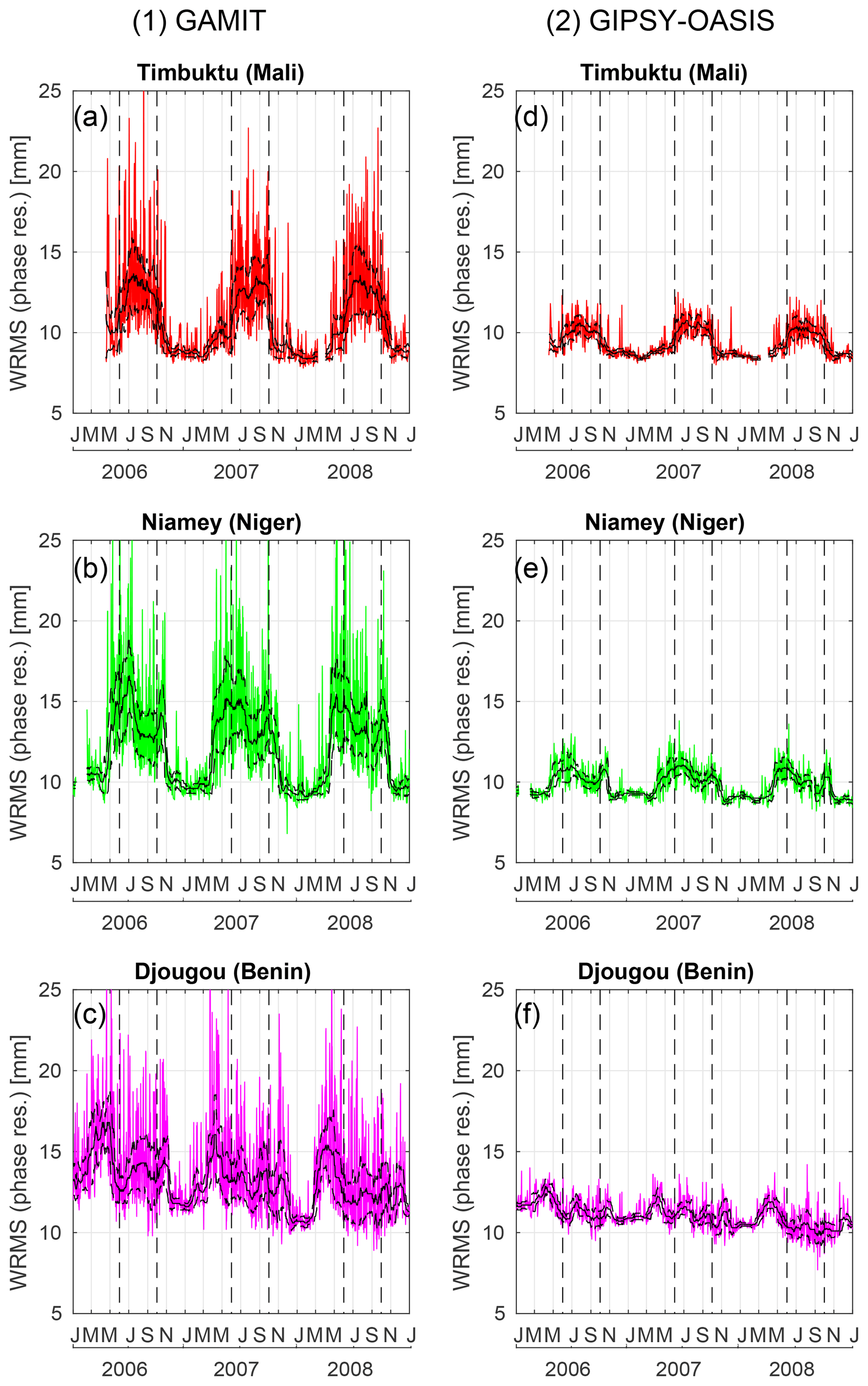
Figure 5 Daily weighted root mean square of the GPS post-fit phase residuals at (a, d) Timbuktu, (b, e) Niamey, and (c, f) Djougou. (a–c) Results of GAMIT software and (d–f) results of GIPSY-OASIS software. The solid black lines show 30 d moving medians, and the dashed black lines show moving median absolute deviations around the medians.

Overall, the analysis of the annual cycle presented in Sect. 2 emphasizes a strong increase in the sub-daily variability of GPS tropospheric estimates (ZWD and gradients) and post-fit phase residuals during the wet season, when the atmosphere is moister and MCSs are observed. In the following section the analysis of a case study allows us to shows how such MCSs generate variability at this fine timescale.

3 Case study of MCS over Niamey, Niger, on 11 August 2006

The MCS that passed over Niamey (Niger) on 11 August 2006 is a typical case of an intense weather event in the Sahel associated with the WAM. It has been the subject of a comprehensive study by Chong (2010) – see also Risi et al. (2010) – and is well-documented by radar and meteorological data. Here, the relevance and limitations of the GPS tropospheric estimates (ZWD and gradients) and post-fit phase residuals during the passage of this MCS are investigated.

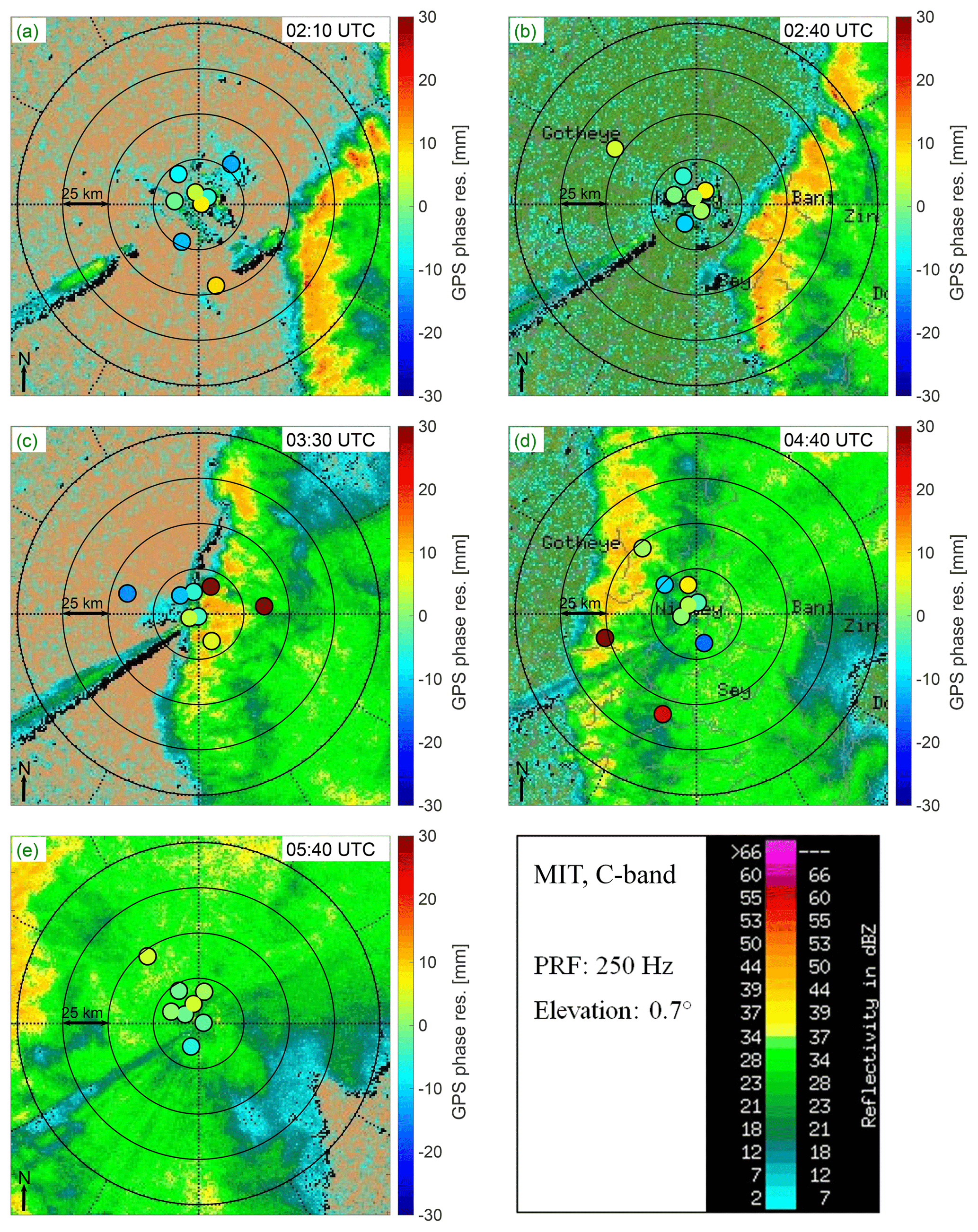
Figure 6 Reflectivity maps from the MIT C-band Doppler radar in Niamey at (a) 02:10 UTC, (b) 02:40 UTC, (c) 03:30 UTC, (d) 04:40 UTC, and (e) 05:40 UTC on 11 August 2006, showing a squall-line MCS approaching from the east and passing straight over the site at 03:30 UTC. Post-fit phase residuals from GPS data processing are superposed on the maps using the GIPSY-OASIS software at the exact times of the radar plots. The radar reflectivity color bar is in the lower right-hand panel. The GPS residual color bar is attached to each panel. The GPS phase residuals are projected on the radar maps in the directions of the satellite-receiver paths, assuming a 10 km troposphere thickness and a spherical Earth with a 6400 km radius. The concentric circles indicate the distance from the GPS station's location at 25 km intervals.

The MCS formed over the border between Chad and Nigeria on the evening of 9 August 2006. It propagated westward, intensified over Nigeria on 10 August, and reached Niamey at 03:15 UTC on 11 August. It was observed from satellite imagery (Fig. 1) approaching Niamey from the east. Figure 6 shows reflectivity maps from the MIT C-band Doppler radar at 02:10 UTC (panel a), 02:40 UTC (panel b), 03:30 UTC (panel c), 04:40 UTC (panel d), and 05:40 UTC (panel e) that illustrate the dynamics of the MCS organized into a commonly observed north–south oriented squall-line. The two parts of the MCS are easily identifiable: the convective part with a reflectivity above than 37 dBZ (in yellow, orange, or red), and the stratiform part, which is more extended, with a reflectivity lower than 37 dBZ (mainly in green). The GPS phase residuals superposed in the figure are discussed later in Sect. 3.3.

3.1 Meteorological surface data

Figure 7 shows surface meteorological data retrieved from the Atmospheric Radiation Measurement (ARM) Mobile Facility (ARM-MF) in Niamey (Miller and Slingo, 2007) at a 1 min sampling interval (black lines) between 00:00 and 08:00 UTC. These sensors are collocated with the AMMA GPS station at the Niamey airport site. The ARM-MF data are preferentially used for this case study because of their accuracy and their higher temporal frequency.

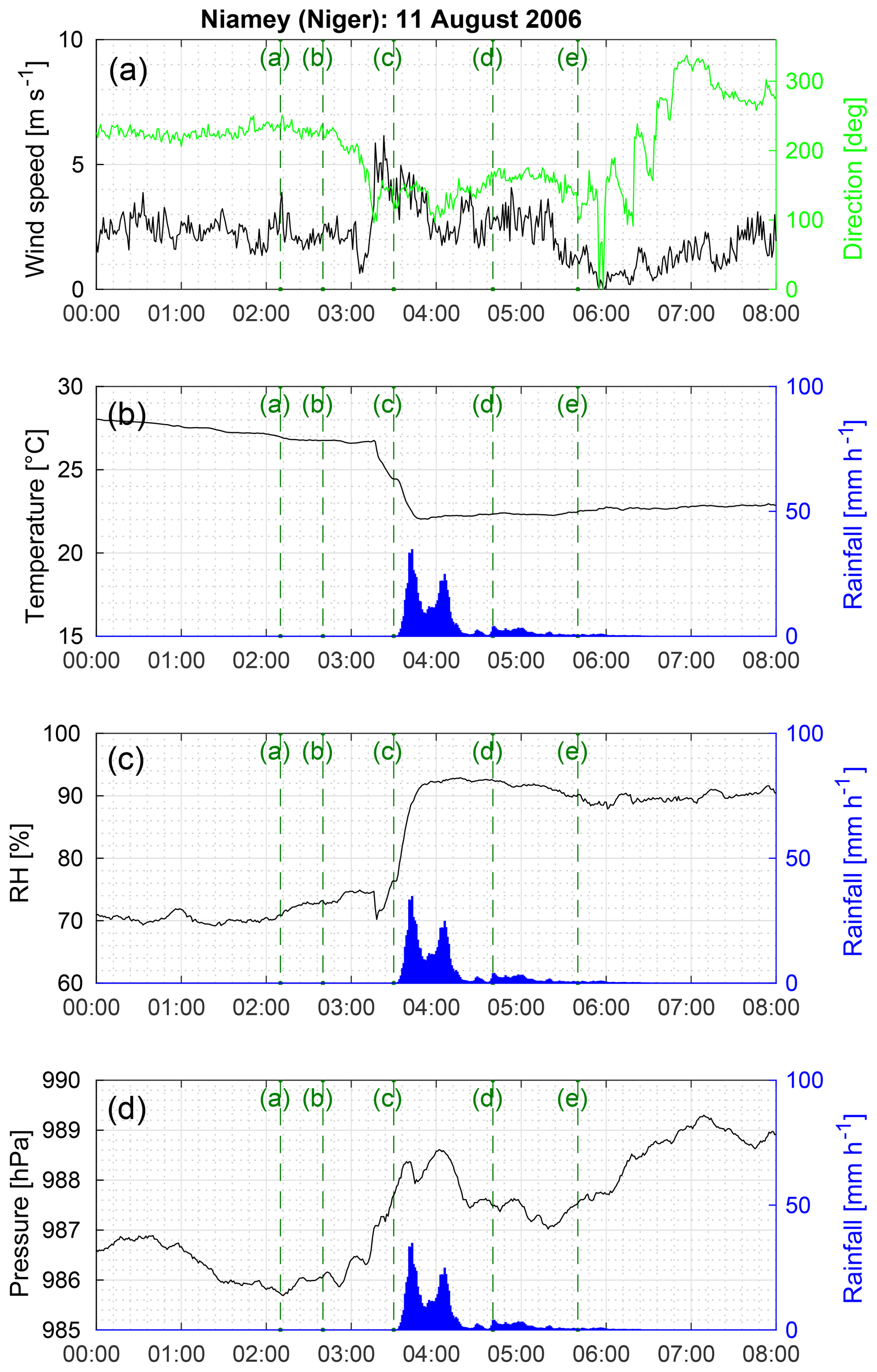
Figure 7 Meteorological data during the MCS event on 11 August 2016 at Niamey (Niger) retrieved from the ARM Mobile Facility at a 1 min sampling interval: (a) wind speed (m s⁻¹) and direction (^∘), (b) temperature (^∘C), (c) relative humidity (%), and (d) pressure (hPa) are shown using black or green lines, and rainfall (mm h⁻¹) is shown using blue bar plots. The times for the reflectivity maps given in Fig. 6 are shown using vertical dashed green lines and correspond to (a) 02:10 UTC, (b) 02:40 UTC, (c) 03:30 UTC, (d) 04:40 UTC, and (e) 05:40 UTC.

Time series of wind speed and direction (Fig. 7a) allow for the arrival of the gust-front preceding deep precipitating convective cells to be precisely detected (e.g., Largeron et al., 2015; Lothon et al., 2011). Provod et al. (2016) associated the cold pool crossing time (CPCT) with the time of a sudden wind direction change that occurs within 5 min or less and reaches at least 30^∘ in magnitude. Between 00:00 and 03:03 UTC, the wind speed varies between 1.5 and 3 m s⁻¹ with a few peaks (not exceeding 4 m s⁻¹) and a direction ranging from 200 to 250^∘. Between 03:03 and 03:18 UTC, it is around 2 m s⁻¹; it then drops to less than 1 m s⁻¹ at 03:06 UTC, and suddenly jumps to 5.8 m s⁻¹ at 03:18 UTC, while the wind direction changes from 200 to 110^∘. The gust-front is detected at 03:16 UTC (Chong, 2010), and the first rainfall is recorded 18 min later at 03:33 UTC with the arrival of a mature deep convective cell. During this period, the wind speed is significantly higher, ranging from 4 to 6 m s⁻¹, it then slightly weakens a few minutes before the first rainfall. The surface temperature rapidly drops from 26.5 to 24.5 ^∘C (Fig. 7b). Similarly, the relative surface humidity suddenly and very briefly drops from 74 % to 70 % within 2 min at the CPCT (Fig. 7c). This time sequence is very typical of the high-frequency fluctuations of surface meteorology observed during the passage of a MCS (e.g., Zipser, 1977). The relative surface humidity then starts rising again before the first rainfall, exceeding 76 % before rainfall occurs.

From 03:33 to 06:41 UTC, the MCS event is characterized by a two-phase rainfall pattern produced successively by its convective and stratiform parts. Between approximately 03:33 and 04:20 UTC, the convective part of the MCS produces heavy convective showers greater than 10 mm h⁻¹ over a cumulative period of 29 min and exceeding 20 mm h⁻¹ over a cumulative period of 12 min. At the beginning of the first shower, a second significant drop in surface temperature, from 24.5 to 22 ^∘C between 03:33 and 03:46 UTC, is observed (Fig. 7b). Likewise, the relative humidity sharply increases to about 92 %. From around 04:20 UTC, the trailing part of the MCS produces stratiform rainfall with a much lower intensity and a much longer duration than convective rainfall: lower than 1 mm h⁻¹ over a cumulative period of 94 min. The wind speed is then weaker (between 2 and 4 m s⁻¹), before it drops to almost 0 m s⁻¹, which, with the cessation of rainfall, marks the end of the MCS event.

Surface pressure also fluctuates during the three major steps of the MCS's lifetime: it increases during the minutes preceding the formation of the convective cell above Niamey; it presents a local maximum during the convective phase; and then it slightly decreases during the stratiform phase. The surface pressure sequence is again consistent with previous studies (e.g., Redelsperger et al., 2002).

There is certainly added value from the high sampling data from the ARM-MF with respect to capturing the details of the internal dynamics of the MCS. However, such data are only available at Niamey (Niger), and only for 2006. The data retrieved from the PTU200 sensor are in good agreement with data from ARM-MF, but the 15 min sampling interval is not sufficient to detect the surface temperature drops (in two consecutive stages) or the sudden and brief drop in relative humidity (not shown). Moreover, because the GPS stations were aimed at providing IWV data, the wind was not recorded. Thus, the best way to identify the CPCT with only PTU200 data at the other AMMA GPS stations is to detect significant drops in surface temperature over a period from 30 min to 1 h before strong rainfall (see Sect. 4).

3.2 GPS estimates

The GPS tropospheric estimates retrieved from the GIPSY-OASIS (black lines) software allows for the MCS to be documented with a 5 min sampling rate (Fig. 8). It includes the estimates from the GAMIT software (red dashed lines). In Fig. 8a, the ZWD is retrieved from the ZTD, and the hydrostatic part is computed using 1 min ARM-MF surface pressure data and by applying the formula from Saastamoinen (1972). Figure 8a also shows the IWV converted from the ZWD using 2 m temperature data and the formula from Bevis et al. (1992). East and north components of the tropospheric gradients are given in Fig. 8c and d, respectively.

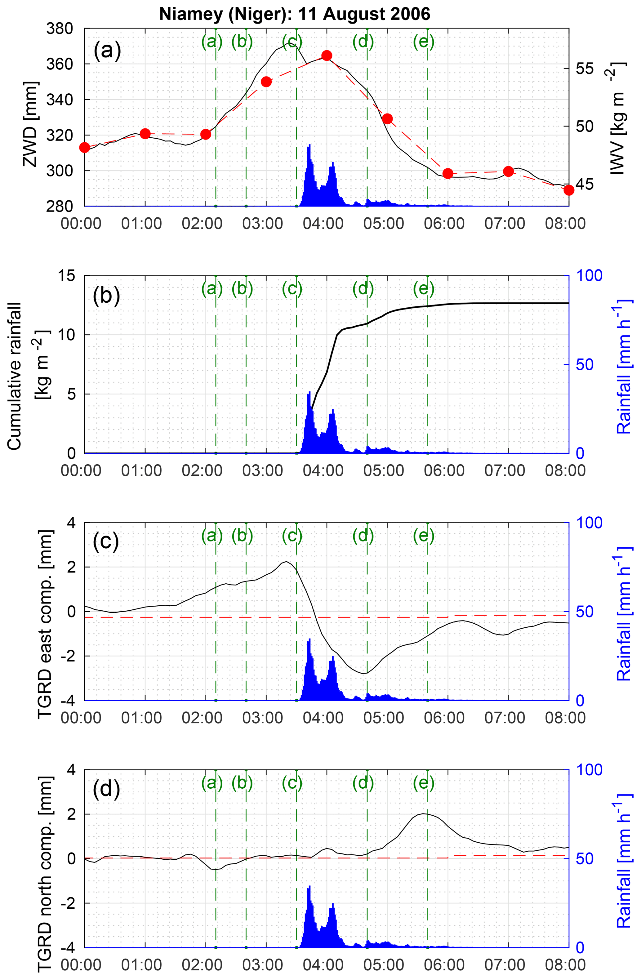
Figure 8 Tropospheric estimates from the GIPSY-OASIS (black solid line) and GAMIT (red dashed line) software packages during the MCS event on 11 August 2016 at Niamey, Niger: (a) zenithal wet delay (mm) and its equivalent IWV (kg m⁻²; red dots), (c) east component of the tropospheric gradients, and (d) north components of the tropospheric gradients (mm). (b) The cumulative rainfall (kg m⁻²; black line) is computed from the 1 min retrieved rainfall (mm h⁻¹; blue bar plots) from the ARM Mobile Facility. Rainfall (mm h⁻¹; blue bar plots) in panel (a) is repeated from  (b)–(d) but is not displayed with a dedicated graduation axis. The times of the reflectivity maps given in Fig. 6 are shown using vertical dashed green lines and correspond to (a) 02:10 UTC, (b) 02:40 UTC, (c) 03:30 UTC, (d) 04:40 UTC, and (e) 05:40 UTC.

Comparing the ZWD estimates retrieved from GAMIT and GIPSY-OASIS (Fig. 8a), good agreement can be seen, such as the ZWD peak coinciding with the rainfall event. However, the 5 min sampled ZWD time series from GIPSY-OASIS reveal finer timescale information. ZWD increases from 315 mm at 01:40 UTC to 372 mm at 03:25 UTC, just a few minutes before the first rainfall (Fig. 8a). It remains above 360 mm from 03:00 to 04:10 UTC, while heavy rainfall concurrently dries out the atmosphere from 03:33 UTC onwards. Over this period, the equivalent IWV is quite stable, between 55 and 57 kg m⁻², while around 10 kg m⁻² of water vapor is extracted from the total column by precipitation (Fig. 8b). The dynamics of the active convective cell involves a low-level convergence of moist air from its immediate environment, which initiates a lift and leads to the significant rainfall amount of 10.5 mm over a 37 min period. As a first approximation, the stability of IWV is well explained by a balance between moisture convergence and precipitation (this implies very minor contributions from surface evaporation and water phase changes to the water budget at this scale). The equilibrium can be broken, e.g., by mixing with drier air in the immediate environment of the cell and/or by processes related to the formation of the incipient convective cells. Such a break occurs around 04:05 UTC – as shown by a decrease in the ZWD followed by a decrease in the precipitation intensity from 04:10 UTC onwards – and marks the transition from the convective part of the MCS to its stratiform part. Between 04:10 and 06:00 UTC, the ZWD decreases from 360 to 297 mm, which corresponds to a decrease of around 9.7 kg m⁻² in the IWV. Over the same period, 2.6 kg m⁻² of atmospheric water is precipitated, which implies that 7.1 kg m⁻² of water has been transported elsewhere, possibly to the newly formed convective cells. Thus, the troposphere is cooler and drier after the passage of the MCS.

Tropospheric gradients retrieved from the GIPSY-OASIS software show the east–west motion dynamic of the MCS between 01:00 and 07:00 UTC. From 01:30 UTC onwards, the east component increases from 0.26 mm and reaches a maximum of 2.25 mm at 03:20 UTC, whereas the north component remains almost null over this same period. The tropospheric gradient vector actually points to the direction of the incoming convective cells and its modulus shows a first local maximum at the CPCT (Fig. 8c, d). This is the time when the anisotropy of the troposphere around the GPS station is the most pronounced (Fig. 6c). Following this, the east component decreases from its maximum to about zero at around 03:48 UTC, when the GPS station is surrounded by convective cells; it decreases to a minimum of −2.79 mm at 04:35 UTC. The modulus of the gradient vector actually shows a second maximum at the end of the motion of the convective zone through the GPS station, when, once again, the anisotropy of the troposphere around the GPS station is the most pronounced (Fig. 6d). At around 05:40 UTC, anisotropy of the stratiform part of the MCS is detected in the northeast direction by gradients, which is confirmed by reflectivity maps (Fig. 6e). Thus, the tropospheric gradients retrieved from the GIPSY-OASIS software appear to be relevant to contribute to the description of the dynamics of intense weather events such as MCSs. Tropospheric gradients retrieved once per 24 h session from the GAMIT software provide no such information, but the examination of the post-fit phase residuals is more informative in this case.

3.3 GPS phase residuals

The daily WRMS computed by the software for the sessions covering the 11 August 2006 are 15 mm with GAMIT and 10 mm with GIPSY-OASIS (see Sect. 2.3.2). In this subsection, we analyze the behavior of the phase residuals during the case study in detail. Therefore, Fig. 9 shows the root mean square (RMS) of the GPS phase residuals computed at a 15 min sampling interval (panel a), the number of GPS observations per epoch (panel b), and the GPS phase residuals (panel c) retrieved from the GIPSY-OASIS (black) and the GAMIT (red) software packages during the MCS event.

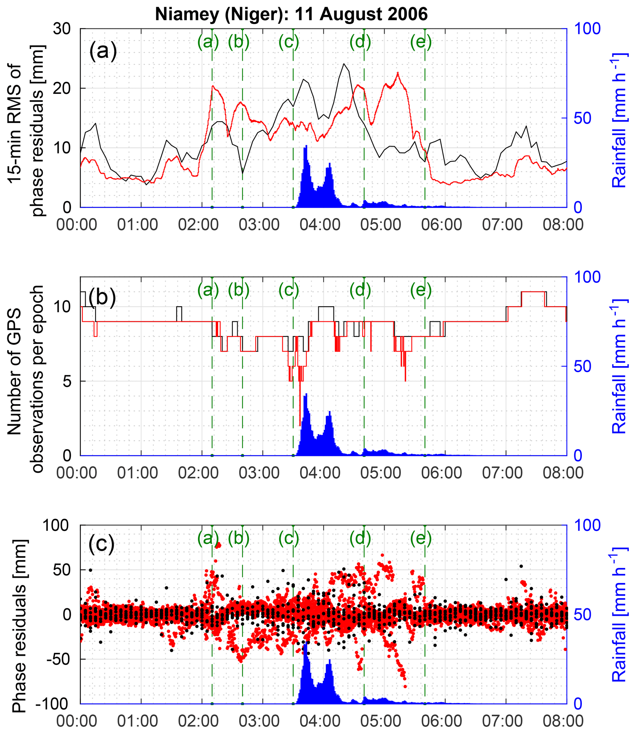
Figure 9 Outputs from GIPSY-OASIS (black) and GAMIT (red) software during the MCS event on 11 August 2016 at Niamey (Niger): (a) the 15 min RMS of GPS phase residuals (mm), (b) the number of GPS observations per epoch and (c) GPS phase residuals (mm) at full temporal resolution (5 min for GIPSY-OASIS and 30 s for GAMIT). Rainfall (mm h⁻¹; blue bar plots) is retrieved from the ARM Mobile Facility. The times of the reflectivity maps given in Fig. 6 are shown using vertical dashed green lines and correspond to (a) 02:10 UTC, (b) 02:40 UTC, (c) 03:30 UTC, (d) 04:40 UTC, and (e) 05:40 UTC.

With GIPSY-OASIS, the 15 min RMS of the GPS phase residuals exceeds 15 mm between 03:10 and 04:35 UTC during the crossover of the convective cells. This indicates that the tropospheric anisotropy is more complex than can be inferred from gradients, which is confirmed by the GPS phase residuals on the reflectivity maps (Fig. 6c). Indeed at 03:30 UTC, the GPS phase residuals exceed 25 mm in the northeast quadrant, are below −10 mm in the northwest quadrant, and are between −7 and 7 mm elsewhere. Before and after this period between 03:10 and 04:35 UTC, the RMS generally oscillates between 5 and 10 mm. Otherwise, the RMS can be slightly higher due to very few mis-modeled and non-deleted GPS observations that produce residuals which are 30 mm over the absolute value (Fig. 9c, black dots). In general, the behavior of the GPS phase residuals reflects the part of the tropospheric anisotropy that cannot be captured by the gradients. This is displayed as spatial correlations in their projected sky-plots (Figs. 6, 10) and is reflected as temporal correlations in their time series (Fig. 9c). Increased scatter in the GPS phase residuals retrieved from GIPSY-OASIS is clearly visible during the MCS event (Fig. 9c), but the 5 min sampling interval of the GPS data does not make easy to detect their temporal correlations. The number of GPS observations per epoch is usually over nine and decreases slightly during the entire event but remains above seven (Fig. 9b). The small number of observations that are rejected indicates that the chosen settings of the GPS data processing with the GIPSY-OASIS software appear to be adequate to study this kind of extreme weather event.

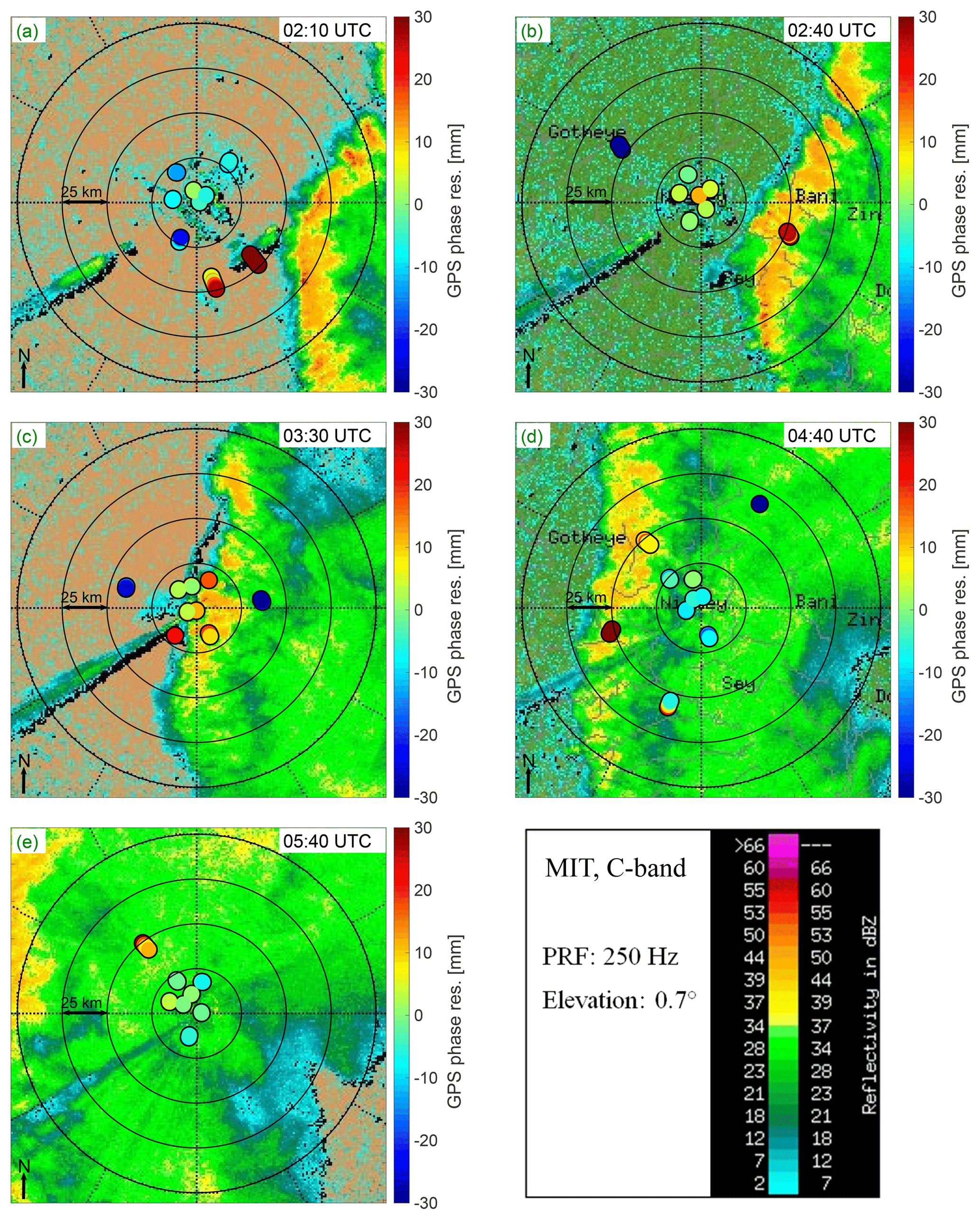
Figure 10 Similar to Fig. 6 but with GPS post-fit phase residuals from the GAMIT processing, with a 30 s sampling interval, over a 5 min span centered on the times of the radar plots.

With the GAMIT software, the RMS of the GPS phase residuals computed at a 15 min sampling interval oscillates between 4 and 8 mm before and after the MCS event (Fig. 9a). It skyrockets as soon as a sufficient number of GPS observations cross the MCS from 8 to 20 mm at 02:00 UTC, then it oscillates between 11 and 22 mm as long as the MCS affects the GPS data. The RMS decreases from over 20 mm at 05:25 UTC to 5 mm at 05:50 UTC while the stratiform part of the MCS is still above the GPS station. Thus, we can assume that the GPS observations that cross the convective part of the MCS are the most disrupted; hence, these observations are poorly modeled during the GPS data processing which leads to higher phase residuals and, in turn, to a higher RMS. Further understanding of the RMS variation while the MCS affects the GPS data is delicate as up to 50 % of the observations per epoch can be rejected as outliers (Fig. 9b, red line). This loss of data has to be put into perspective: the 30 s sampling interval of the GPS data processed by GAMIT leads to the processing of 10 times more data than with GIPSY-OASIS – thus, many more residuals are available for study (Fig. 9c, red dots). Strong deviations in the phase residuals are clearly visible during the MCS event on some satellites as revealed by temporally correlated patterns. Therefore, we examined the projected GPS phase residuals from GAMIT and superimposed them onto the reflectivity maps retrieved from the MIT C-band Doppler radar (Fig. 10).

Assuming a tropospheric thickness of 10 km and a spherical Earth with a radius of 6400 km, the GPS phase residuals are projected on a horizontal plane of the local coordinate system centered on the GPS station to be approximately superimposed on the reflectivity maps retrieved from the MIT C-band Doppler radar. The results obtained at 02:10 UTC (panel a), 02:40 UTC (panel b), 03:30 UTC (panel c), 04:40 UTC (panel d), and 05:30 UTC (panel e) are given by Fig. 6 for GIPSY-OASIS and by Fig. 10 for GAMIT.

At 02:10 UTC, the GPS phase residuals exceed 20 mm in the southeast direction because the associated GPS observations are disturbed by the top of the MCS's anvil, which can not be detected by the radar waves at an elevation of 0.7^∘. Between 02:10 and 03:00 UTC, the GPS phase residuals within a radius of 25 km are within an acceptable range; however, beyond 25 km, GPS phase residuals located to southeast indicate the presence of convective cells and exceed 20 mm, while those located in other directions are below −20 mm (Fig. 10b). At 03:30 UTC, convective cells are above the GPS station and GPS phase residuals are very disturbed within a radius of 25 km, while those beyond 25 km located to the east or west are below −20 mm (Fig. 10c). At 04:40 UTC, convective cells are located west of the station. The GPS phase residuals within a radius of 25 km are negative but stay in an acceptable range, whereas those corresponding to signals going through the convective cells always exceed 20 mm. At 05:40 UTC, the GPS phase residuals located to the northwest exceed 20 mm which explains the signal detected in the north component of the tropospheric gradients in the previous subsection. Thus, with the GAMIT solution, the tropospheric anisotropy induced by the MCS is mainly reflected in GPS phase residuals, and the east–west crossing of the MCS can be detected in the temporal evolution of the extreme phase residuals in the maps of the Fig. 10. However, for a more quantitative study, the tropospheric gradients retrieved by GIPSY-OASIS would be more accurate.

4 Composites of surface variables and GPS estimates during MCS events over West Africa

Section 3 provided a detailed analysis of a single case study. Here, we aim to characterize the West African MCS properties in a systematic way using the data from the six AMMA GPS stations over three monsoon seasons, between 2006 and 2008.

4.1 Detection of MCS at AMMA GPS stations

A crucial step is to define a method to properly detect MCSs based on surface meteorological data. Provod et al. (2016) used 1 min averaged pressure, temperature, and wind observations from the ARM-MF in Niamey to detect the arrival of cold pools associated with MCSs, which they subjectively verified from the MIT radar and/or Meteosat satellite images. They detected 42 cold pools during the Special Observing Period (SOP) of the AMMA project (1 June–30 September 2006). Among them, 33 were squall-line MCSs, 4 were non-squall-line MCSs, 1 was from a freshly dissipated MCS, and 4 were from local non-MCS convection.

As in the study by Provod et al. (2016), here we use a method of detecting cold pools based on surface meteorological data. These data, available from the PTU200 sensors attached to the AMMA GPS stations, include pressure, temperature, and relative humidity (recorded with a sampling rate of 15 min), but no wind data. First, we primarily detect rainfall events and then select those that show the surface air temperature drop characteristics of the arrival of cold pools ahead of the MCS's peak rain rate. The first detection step is fundamental because substantial rainfall implies the presence of significant cloud cover which attenuates the variations of the surface temperature due solar radiation and thus avoids false detections and fails due to the daily solar cycle.

The quality of the PTU200 data was first assessed by comparison with the ARM-MF data at Niamey. The mean ± one standard deviation of differences in pressure, temperature, and relative humidity were 0.0 ± 0.1 hPa, 0.4 ± 0.8  ^∘C, and 0.6 ± 1.9 %, respectively. The rain rate data were retrieved from the 3-hourly, $\mathrm{0.25}{}^{\circ }\times \mathrm{0.25}$^∘ gridded precipitation data (3B42 v6) from the Tropical Rainfall Measuring Mission (TRMM) Multisatellite Precipitation Analysis (Huffman et al., 2007). The TRMM rain rates were compared point to point to the ARM-MF data at a 3 h sampling interval (2972 points). Rainfall was detected at 243 points by either TRMM or ARM-MF data but only at 74 points in both data sources. At the 169 remaining points, rainfall was observed either only by TRMM or only by ARM-MF. At 145 points from the 169 (86 %), the rain rate was less than 0.5 mm h⁻¹. The 16 remaining points (14 %) corresponded to more intense rainfall, but it was observed at different times. This result led us to define a rainfall event as an uninterrupted period of precipitation during which the maximum rain rate is higher than 0.5 mm h⁻¹.

We detect 27 events using the 3 h ARM-MF rainfall data during JJAS 2006 and 47 events using the TRMM rainfall data. Among the 27 ARM events, 25 coincided with at least one TRMM rainfall event. The two ARM events not detected by TRMM are of very low intensity and most probably correspond to small local showers. Each event is associated with a start time, a time of maximum precipitation, and an end time. If several rainfall events occur within a 13 h window they are merged together as we are mainly interested in MCSs events in which several convective cells can be detected. We keep the rainfall events with average precipitation above 0.5 mm h⁻¹ and with a peak rain rate above 1 mm h⁻¹. This method detects 27 events from the TRMM data and 20 events from the ARM-MF rainfall data. Compared with the first intercomparison, the agreement between the two datasets is improved when considering longer and more intense events. The seven TRMM events that do not match with any ARM-MF rainfall event may be due to the difference in the spatial representativeness of rainfall between the two datasets: very localized for ARM data and more extended for TRMM data ($\mathrm{0.25}{}^{\circ }\sim \mathrm{30}$ km). As the GPS tropospheric estimates are sensitive to weather events occurring within a radius of approximately 75 km around the station (as illustrated in Figs. 6 and 10), we actually expect better agreement with the TRMM observations than with local precipitation observations.

For the detection of MCSs, we identify the CPCT by seeking and dating the largest temperature drop over 1 h within a time window defined from the event start time minus 4 h to the event end time plus 3 h. To detect a cold pool associated with a MCS, the temperature drop must be at least 1 ^∘C, as in Provod et al. (2016).

Figures 11 and 12 show the events detected using our method on Niamey data during August 2006 along with surface meteorological observations from the PTU200 sensor and ARM-MF data (Fig. 11) and GPS tropospheric estimates (Fig. 12) retrieved with both software approaches (GIPSY-OASIS as black lines and GAMIT as red dashed lines). The method detects 10 MCS events based on the rain rates from TRMM data (Fig. 11c, d) and temperature from the PTU200 (Fig. 11b). In general, all of the detected MCS cases were confirmed from the reflectivity maps of the MIT C-band Doppler radar. One event (14 August 2006) is not detected in the ARM-MF rain rate data. This event is actually a propagating cold pool from a freshly dissipated MCS (Provod et al., 2016). All periods detected include a rapid increase in the wind speed associated with a sudden change of direction (Fig. 11a), which are the characteristics of the arrival of a cold pool. They also include a pronounced and sudden drop in temperature (Fig. 11b), and an increase in relative humidity (Fig. 11c) and ground pressure (Fig. 11d). This is all consistent with previous studies (e.g., Redelsperger et al., 2002). There is also a clear peak in the ZWD (Fig. 12a), a signal in the tropospheric gradients retrieved from GIPSY-OASIS (Fig. 12b, c), and an increase in the 15 min RMS of GPS phase residuals retrieved from GAMIT (Fig. 12d). Careful inspection of the wind, temperature, tropospheric gradients, and phase residuals reveals two potential events with cold-pool-like signatures on 30 and 31 August that were not detected because there was no signal in rainfall. Furthermore, there is no peak in the ZWD data associated with these potential events (Fig. 12a). Inspection of the MIT radar data actually shows decaying MCSs for these two cases.

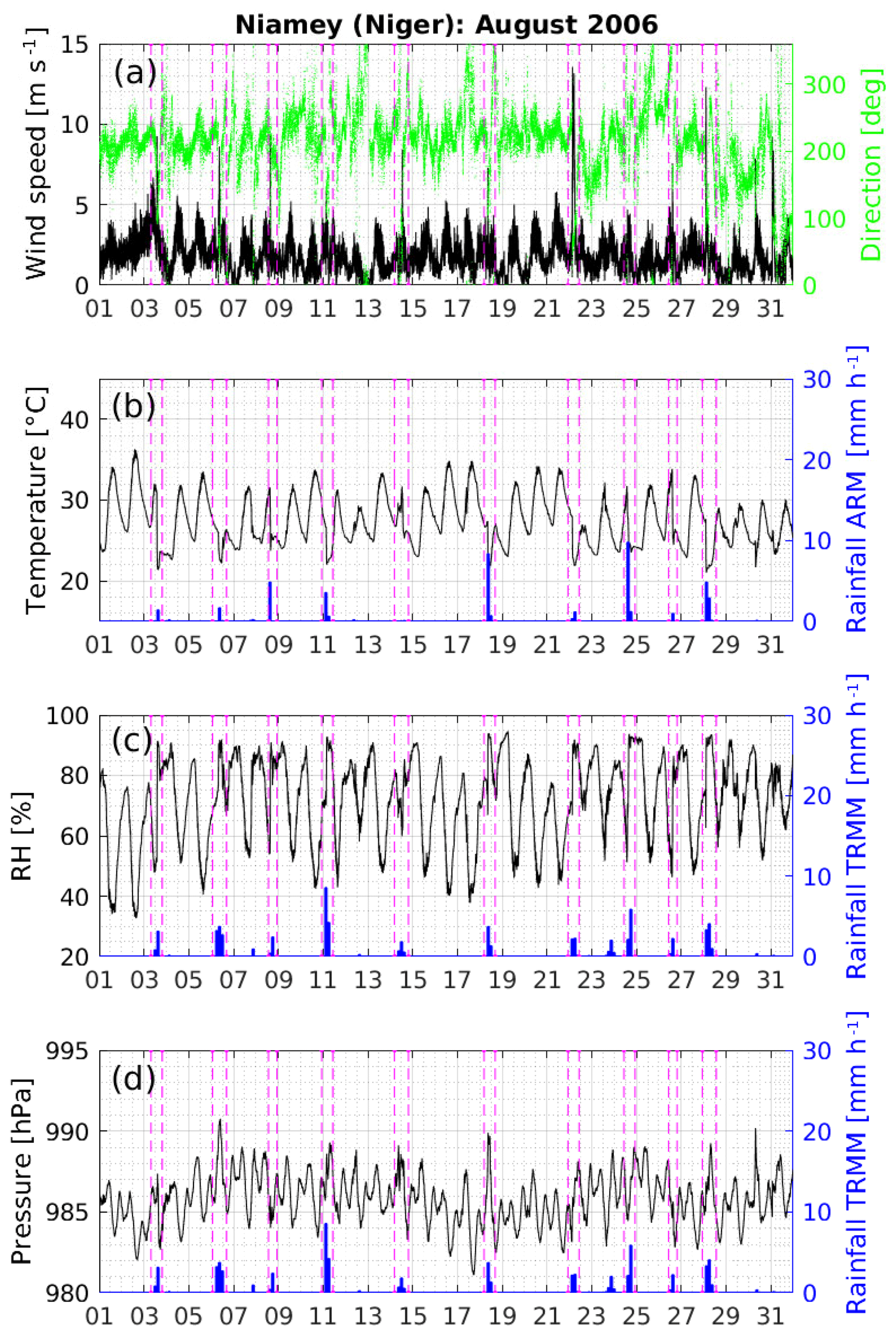
Figure 11 Surface meteorological data from the ARM Mobile Facility with a 1 min sampling interval (black or green lines) at Niamey during August 2006: (a) wind speed (m s⁻¹) and direction (^∘), (b) temperature (^∘C), (c) relative humidity (%), and (d) pressure (hPa). The 3 h rainfall (mm h⁻¹; blue bar plots) is retrieved (b) from the ARM Mobile Facility and (c, d) from the TRMM Multisatellite Precipitation Analysis. Each MCSs detected is shown using two dashed vertical dashed magenta lines indicating the start and end of the rainfall period.

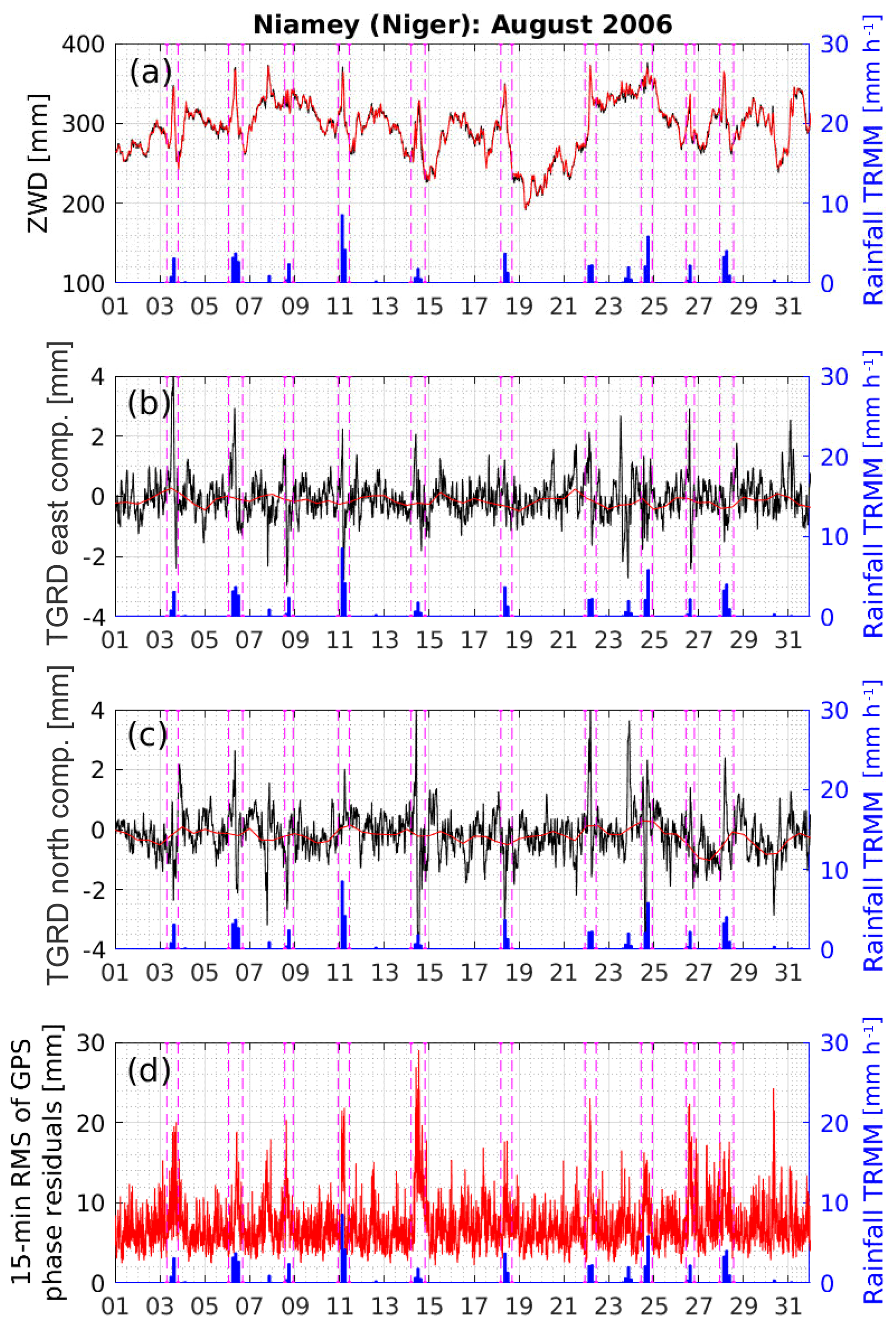
Figure 12 Tropospheric estimates from GIPSY-OASIS (black) and GAMIT (red) at Niamey during August 2006: (a) zenithal wet delay (mm), (b) east and (c) north components of tropospheric gradients (mm), and (d) the 15 min RMS of GPS phase residuals (mm). Each MCS detected is shown using two dashed vertical magenta lines indicating the start and end of the rainfall period.

Thus, of the 42 cold pools detected and categorized by Provod et al. (2016), the detection procedure retains the 24 most intense ones including large MCSs, mainly squall-lines, over the JJAS period in 2006. The MCS detection procedure was then applied to the six AMMA GPS stations over the JJAS periods from 2006 to 2008. We note that precipitation and lightning from the ground, as well as from clouds and lightning from geostationary satellites could be added to the MCS detection arsenal. This additional information will be considered in the future.

4.2 Composites of meteorological variables and GPS estimates during MCS events in JJAS from 2006 to 2008

Using the detection method described in Sect. 4.1, we flagged a total of 414 MCSs passing over the six AMMA GPS stations in JJAS from 2006 to 2008. The detailed characteristics for each event (start, peak, and rainfall end times, CPCT, temperature drop, and precipitation peak and cumulative rainfall depth) are given in the Supplement. The list only includes events for which both PTU200 and GPS data were available within the 10 h windows centered on the CPCTs (i.e., a few events may not be documented because of gaps in our data).

Table 3 Statistics (mean ± one standard deviation) for 414 MCS events detected at the AMMA GPS stations during JJAS from 2006 to 2008. Characteristics of the atmospheric environment before the MCS: surface air temperature, pressure, and relative humidity from PTU200 sensors, and ZWD from GPS receivers (these variables are averaged over the 5 h before the cold pool crossing time). Cumulative rainfall depth and the maximum rain rate from the TRMM Multisatellite Precipitation Analysis (Huffman et al., 2007). The last column gives the maximum temperature drop, ΔTemp, within the 1 h following the cold pool crossing time.

^∗ The number of events detected at TAMA is smaller because of a long gap in the GPS data in 2007.

Table 3 reports the number of events and the statistics of the surface air variables, precipitation, and ZWD recorded by the six stations. The meridian climatic gradient between the Sahara and the Guinean coast is reflected in both the number of MCS events and the atmospheric variables. The number of events ranges from 31 in Timbuktu to 116 in Djougou, i.e., with a ratio of 1:4. Note that the number of events detected at Tamale is smaller due to failures with the GPS receiver in 2007. The atmospheric environment of these MCSs is characterized using the surface air temperature, pressure, and relative humidity, and the ZWD. Again, the meridional climatic gradient is clearly reflected in these variables. Surface air temperature and relative humidity range from the very hot (over 34 ^∘C) and dry (below 45 %) Saharo–Sahelian climate to the milder (below 30 ^∘C) and moister (over 69 %) Sudano–Guinean climate. The mean surface pressure is not very informative here as it mainly reflects the altitude of the station, but variability is seen to be stronger at the Sahelian sites (Niamey, Gao, and Timbuktu). A contrast is also seen in the ZWD values that are below 270 mm at Timbuktu and Gao and above 290 mm at the other sites. The ZWD characterizes the total column water vapor which is, as expected, lower on average and shows a stronger variability in Mali than at the southernmost sites. However, the relative contrast between the ZWD values is not as strong as the contrast between the surface relative humidity values. Surface humidity is strongly controlled by surface evapotranspiration, which is a more limiting factor due to the relatively low soil moisture content and vegetation cover in the Sahel (Lohou et al., 2014), whereas ZWD is largely influenced by upper level moisture transport, which is more of a large-scale nature – e.g., synoptic-scale fluctuations induced by African easterly waves can be quite large at the northernmost sites (Barthe et al., 2010). In the south, the lower saturation vapor pressure due to relatively cooler air is also a limiting factor to both surface humidity and the ZWD. In line with Lebel et al. (2003) and Frappart et al. (2009), rainfall characteristics also show marked latitudinal variations, with a minimum cumulative rainfall of around 10 mm at the Saharo–Sahelian stations (Timbuktu and Gao) and a maximum at the Sudano–Sahelian stations (16 and 21 mm at Niamey and Ouagadougou, respectively). Interestingly, the Saharo–Sahelian stations show the most important surface air temperature drop (around −8 ^∘C in 1 h on average); this reflects the strong cooling (and moistening) of the cold pool air (Lothon et al., 2011; Provod et al., 2016) when it enters the typically warmer and drier boundary layer. Figures 13 and 14 show composites of the surface meteorological variables, the ZWD, and the tropospheric delay gradient components, centered on the CPCT of the MCSs for all six AMMA stations. Overall, the variables show similar temporal variations at all of the sites. The variations are also highly consistent with those observed in the 11 August case study presented in Sect. 3: a drop in surface air temperature coincident with a jump in relative humidity and in surface pressure, as well as a gradual increase in the ZWD that peaks slightly after (∼30 min) the CPCT. The east gradient component also shows a systematic oscillation across the CPCT, whereas the north gradient is more stationary throughout the time window. There is a clear increase of the magnitude of all changes around the CPCT with the latitude of the site (along the south–north climate gradient). Surface air temperature (Figs. 13a, 14a) and relative humidity (Figs. 13b, 14b) do not fluctuate much before and after the CPCT. The magnitudes of the relative humidity and surface pressure jumps are coupled with the magnitudes of the temperature drops. They reach over 30 % RH and 2 hPa at Gao and Timbuktu, compared with only 15 %–20 % and 1 hPa at Djougou and Tamale. Small trends in these variables can actually be seen after the CPCT at the four northernmost sites and reveal a gradual drying and warming of the surface air after the passage of MCSs.

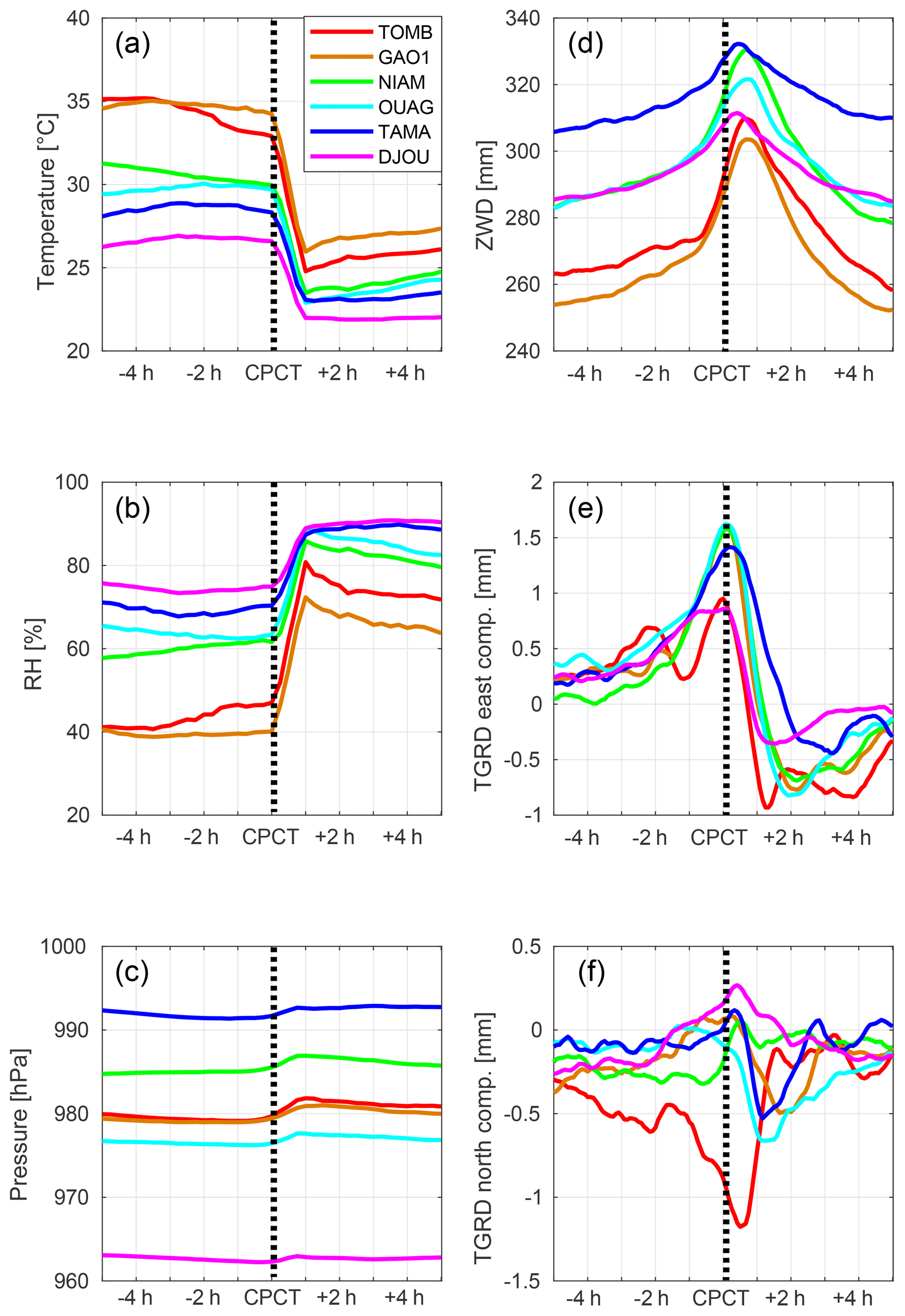
Figure 13 Composites of surface air (a) temperature (^∘C), (b) relative humidity (%), and (c) pressure (hPa) from the in situ PTU200 sensor, and (d) the ZWD (mm), (e) east components of the tropospheric delay gradient, and (f) north components of the tropospheric delay gradient (mm) at all six AMMA stations, in a 10 h window centered on the cold pool crossing time (CPCT).

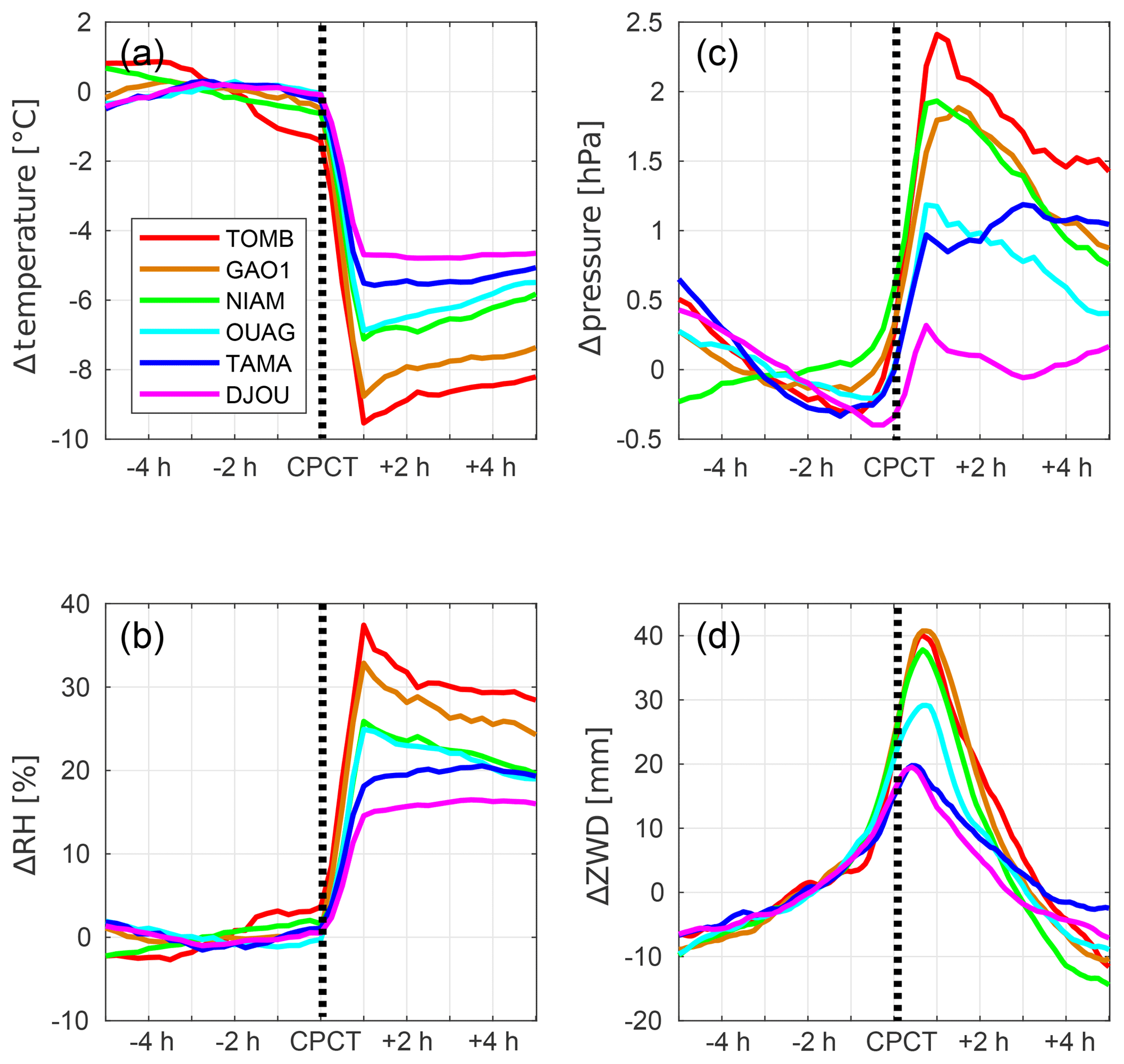
Figure 14 Same as Fig. 13 but variables are differentiated by the average values computed over the 5 h period preceding the cold pool crossing time (CPCT). The average values are given in Table 3.

Figure 14d shows that the ZWD starts to increase 5 h before the CPCT at a common rate of around 3 mm h⁻¹. In the 30 min before the CPCT, this rate increases, and it is only then that it depends on the latitude of the station. The lowest rates of 8 mm h⁻¹ are found at Djougou and Tamale, and the highest rates of 16 mm h⁻¹ are seen at Niamey, Gao, and Timbuktu. The ZWD peaks ∼30 min after the CPCT at all sites. Thus, the change in the ZWD is strongly station (latitude) dependent: it is more marked at the northernmost stations where it reaches around 40 mm (relative to a reference value taken 2 h before the CPCT); it reaches 30 mm at Ouagadougou; and it only reaches 20 mm at the southernmost sites. Hence, moisture convergence associated with the propagating MCSs is larger in the initially drier Saharo–Sahelian atmospheres than in the moister Guinean region. At CPCT plus 5 h, the ZWD has generally decreased back to or slightly below its initial value. Although there is a strong moisture convergence associated with the passage of the MCS, the tendency after it is a slightly drier air column, especially in the more arid climate (this is consistent with typical signatures found in sounding data, not shown). The ZWD peak is also relatively narrow (less than 12 h), and it is narrower from the southern to the northern sites, which suggests faster MCSs in the north (and is again consistent with existing studies, e.g., Maranan et al., 2018). It also implies that the moisture convergence occurs at sub-synoptic scales.

The isotropic vision of water vapor changes in the atmospheric column described by the ZWD time series is complemented by tropospheric gradients which reflect the horizontal displacement of MCSs around the GPS stations. The east component (Fig. 13e) has a very similar behavior at all AMMA GPS stations. It is very low at CPCT minus 5 h and slightly increases to show a maximum at the CPCT when the anisotropy of the troposphere around the GPS station is most pronounced. It then decreases rapidly to present a minimum during the 1–2 h following the CPCT, which corresponds to the east–west crossing of the convective part of the MCSs. After this minimum, the east component tends to return to a value close to zero, corresponding to the passage of the stratiform part of the MCSs. The behavior of the east component previously observed in Sect. 3.2 seems to be common to all GPS stations in West Africa during the passage of MCSs, implying that MCSs preferentially propagate in the east–west direction (which is very consistent with numerous past studies, e.g., Mathon and Laurent, 2001). Conversely, the north component of the tropospheric gradients (Fig. 13f) does not show such a systematic behavior. It would be valuable to assess whether these differences in the meridional direction agree with findings from MCS tracking (using satellite data). A stronger signal is found at Timbuktu where this component remains negative on average throughout the time window. This suggests that convective cells pass preferentially south of the station, which is a result that may be related to the location of the site, on the northern flank of the intertropical convergence zone (ITCZ). The signal is distinct and also weaker at all of the other stations. However, it is noticeable that it is very similar at Niamey to the one observed for the case study (Fig. 8), which suggests that convective cells have a slight tendency to arrive at the station from the southeast and then turn west.

5 Conclusions

The characteristics of GPS tropospheric estimates (ZWD and gradients) and post-fit phase residuals during the wet season (June to September) of the West African monsoon were evaluated using two different GPS data processing approaches. The first uses the double-difference observations from a regional network of GPS stations centered on the study area (West Africa) with the GAMIT software. The second uses the undifferenced observations in PPP mode with the GIPSY-OASIS software. Hourly ZWD estimates retrieved using both strategies are highly consistent on average (RMS difference of ∼4 mm). Both processing solutions exhibit a strong seasonal modulation of the ZWD and gradient variability reflecting the presence of active moisture transport during the monsoon period. In this respect, the 5 min sampling interval of the ZWD and gradient estimates with GIPSY-OASIS appears to be more suitable for studying rapid weather events compared with the 1-hourly ZWD and daily gradient sampling of GAMIT. Sub-daily gradient variability is shown to be quite large (1σ of 0.6 mm on average with peaks up to 2 mm) and to represent a strong source of uncertainty in the GAMIT estimates. Mis-modeling of the tropospheric delay variability in the GAMIT solution is reflected in the post-fit residuals during the monsoon season (the weighted RMS of residuals passes from 10 mm during the dry season to 15 mm on average during the wet season). Mesoscale convective systems (MCSs) are a major contributor to the rapid tropospheric delay anisotropy.

The case study of the squall line over Niamey on 11 August 2006 confirmed the good sensitivity of both GPS software packages to the ZWD variation associated with the passage of a MCS. In this case, a rapid increase of 40 mm was observed in the ZWD over the 2 h preceding the rainfall peak followed by a decrease leading to a slightly lower final ZWD value (20 mm below the initial value). Thanks to the high temporal sampling of the gradient estimates, the GIPSY-OASIS solution provides additional information on the atmospheric anisotropy. The east gradient component shows a strong oscillation reflecting the westward propagation of the MCS passing over the station. With the GAMIT solution, the horizontal anisotropy is reflected to some extent in the post-fit residuals, as could be verified on reflectivity maps from the MIT C-band Doppler radar.

These results were extended by the analysis of composites of surface meteorological variables and GPS delay estimates at all six AMMA stations over three monsoon seasons (2006–2008). It shows a very consistent behavior in all variables during the time window of ±5 h around the cold pool crossing times (CPCTs) of all 414 MCS events. Qualitatively, all MCS events show a drop in the surface air temperature and a jump in the relative humidity and pressure at the CPCT consistent with the squall-line case study and the results of Provod et al. (2016) for Niamey. Quantitatively, however, there is a clear tendency toward a stronger magnitude of the changes at higher latitude, i.e., a dependance on the atmospheric environment specific to each site. The dry Saharo–Sahelian climate of Gao and Timbuktu is prone to the steepest surface temperature drops (−9 ^∘C) and increases in ZWD (40 mm, i.e., about 6 kg m⁻² IWV) due to moisture convergence close to the time when the cold pool arrives. However, cumulative rainfall (10 mm) and the peak rain rate (3 mm h⁻¹) are lower in this region than at the Sudano–Sahelian sites of Ouagadougou and Niamey. This may be due to the stronger evaporation of rainfall drops (Meynadier et al., 2010a) in drier climates. Furthermore, at this scale the total column moisture shows a tendency to diminish after the passage of the MCS, indicating that the balance between moisture convergence and precipitation is negative; however, the opposite is actually seen at the moist Soudano–Guinean sites (Djougou and Tamale). Finally, the tropospheric gradients show that the main direction MCS propagation at all six sites is from east to west, which is consistent with climatology based on the satellite imagery (e.g., Laing and Fritsch, 1993).

To conclude, this study showed that the high frequency estimates of the ZWD and the tropospheric delay gradients are relevant for climate monitoring and the documentation of intense weather events such as MCSs. They could also be used to study other rapid meteorological processes and for verification and assimilation in numerical weather prediction models.