The sensitivity of oceanic precipitation to sea surface temperature

Our study forms the oceanic counterpart to numerous observational studies over land concerning the sensitivity of extreme precipitation to a change in air temperature. We explore the sensitivity of oceanic precipitation to changing sea surface temperature (SST) by exploiting two novel datasets at high resolution. First, we use the Ocean Rainfall And Ice-phase precipitation measurement Network (OceanRAIN) as an observational along-track shipboard dataset at 1 min resolution. Second, we exploit the most recent European Reanalysis version 5 (ERA5) at hourly resolution on a 31 km grid. Matched with each other, ERA5 vertical velocity allows the constraint of the OceanRAIN precipitation. Despite the inhomogeneous sampling along ship tracks, OceanRAIN agrees with ERA5 on the average latitudinal distribution of precipitation with fairly good seasonal sampling. However, the 99th percentile of OceanRAIN precipitation follows a super Clausius–Clapeyron scaling with a SST that exceeds 8.5 % K⁻¹ while ERA5 precipitation scales with 4.5 % K⁻¹. The sensitivity decreases towards lower precipitation percentiles, while OceanRAIN keeps an almost constant offset to ERA5 due to higher spatial resolution and temporal sampling. Unlike over land, we find no evidence for a decreasing precipitation event duration with increasing SST. ERA5 precipitation reaches a local minimum at about 26 ^∘C that vanishes when constraining vertical velocity to strongly rising motion and excluding areas of weak correlation between precipitation and vertical velocity. This indicates that instead of moisture limitations as over land, circulation dynamics rather limit precipitation formation over the ocean. For the strongest rising motion, precipitation scaling converges to a constant value at all precipitation percentiles. Overall, high resolutions in observations and climate models are key to understanding and predicting the sensitivity of oceanic precipitation extremes to a change in SST.

1 Introduction

The equilibrium water vapor pressure increases with temperature, as described by the Clausius–Clapeyron (CC) equation, by about 7 % K⁻¹ (e.g., Trenberth et al., 2003; Held and Soden, 2006). The same CC scaling of a 7 % K⁻¹ atmospheric moisture increase has also been found in modeling studies (Stephens and Ellis, 2008; Allan et al., 2014) and observations (Wentz and Schabel, 2000; Simmons et al., 2010; O'Gorman et al., 2012). Willett et al. (2010) report a global change of 7.3 % K⁻¹ for global humidity observations from 1973 to 1999. As more atmospheric moisture can lead to stronger precipitation events, a similar scaling relation for precipitation is expected; however, the actual rate of change in precipitation with warming is still uncertain, and this is what this study addresses over the ocean.

Despite being studied for some years, the uncertainty in the rate of change for precipitation exceeds that of the atmospheric moisture content because radiative constraints rather than moisture availability limit precipitation. Estimates for the change in global mean precipitation range between 1 and 3 % K⁻¹ (Allen and Ingram, 2002; Arkin et al., 2010; Allan et al., 2014). Over the global land area, there is medium confidence that precipitation increased during the second half of the 20th century, while high confidence is found for the Northern Hemisphere midlatitudes (IPCC, 2014a). At regional scales and for sub-daily precipitation estimates, some studies find changes strongly exceed 10 % K⁻¹ (Lenderink and van Meijgaard, 2008, 2010). How widespread such cases of super CC scaling occur is under debate (Haerter and Berg, 2009; Lenderink et al., 2017). Hardwick Jones et al. (2010) find a positive scaling for sub-hourly precipitation rates over Australia between 20 and 26 ^∘C, while they find a negative scaling above 26 ^∘C due to moisture limitations. Utsumi et al. (2011) reveal latitudinal differences of CC scaling as well as marked differences between daily and sub-daily to sub-hourly precipitation rates. Accordingly, resolution plays a crucial role in the scaling of precipitation over land with surface temperature.

Unlike over land, it remains widely unknown how precipitation scales with sea surface temperature (SST) over the ocean, particularly at sub-daily resolution, though the ocean covers more than 70 % of the Earth's surface and receives 77 % of its precipitation (Schmitt, 2008). As a consequence, no long-term records of precipitation exist over the ocean (IPCC, 2014b; Maggioni et al., 2016). The few existing shorter datasets are often limited by measurement quality, sparse data coverage and low temporal resolution.

Under the challenging oceanic conditions with high wind speeds of varying direction and sea state, optical disdrometers have been recommended as a reference in situ instrument to measure precipitation (Taylor, 2000; Weller et al., 2008). Since 2010, the Ocean Rainfall And Ice-phase precipitation measurement Network (OceanRAIN; Klepp et al., 2018) has provided high-quality in situ oceanic precipitation data from optical disdrometers at 1 min resolution. We use this dataset in combination with the most recent European Re-Analysis version 5 (ERA5) of the European Centre for Medium-Range Weather Forecasts (ECMWF) to investigate the sensitivity of oceanic precipitation to changing SSTs.

In addition to thermodynamic drivers such as SST, dynamic drivers as part of the general atmospheric circulation strongly control if and how much precipitation is formed in the atmospheric column. Emori and Brown (2005) find an overall increase in mean and extreme precipitation, mainly due to thermodynamic changes while dynamics tend to diminish precipitation, particularly in the subtropics. Changes in extreme precipitation are particularly important as they account for most of the accumulation. To shed light on observed changes in extreme precipitation with SST we constrain extreme precipitation from OceanRAIN by the circulation regime using vertical velocities from ERA5.

The paper starts by introducing the datasets and the methods used. First, we investigate the OceanRAIN sampling and how precipitation intensities change with latitude. Second, we consider the change of different precipitation percentiles with respect to a change in SST. Third, we investigate the distribution of vertical velocity in ERA5 and use it to exclude regions of low correlation between precipitation and vertical velocity. We also compare OceanRAIN with ERA5 for the same vertical-velocity regime (lifting air mass). Fourth, we consider how the precipitation event duration changes with SST. The last chapter summarizes our findings and presents some concluding thoughts and next steps.

2 Data and methods

2.1 Data

OceanRAIN

The Ocean Rainfall And Ice-phase precipitation measurement Network (OceanRAIN; Klepp, 2015; Burdanowitz et al., 2016; Klepp et al., 2018) provides water-cycle-related and energy-cycle-related parameters from June 2010 to April 2017 over the global ocean, collected onboard eight research vessels (RVs). In OceanRAIN version 1.0 (OceanRAIN-W; Klepp et al., 2017), the RVs include the German RVs Polarstern (since June 2010), Meteor (since March 2014), Maria S. Merian (October 2012 to June 2014) and Sonne (September to October 2012) as well as its successor Sonne II (since November 2014). The Australian RV Investigator (January to February 2016) and the American RV Roger Revelle (August to September 2016) contributed temporarily to OceanRAIN. Klepp et al. (2018) describe the post-processing and quality-checking of the OceanRAIN data in detail. OceanRAIN is publicly available free of charge: more information can be accessed at https://oceanrain.cen.uni-hamburg.de/index.php?id=2752 (last access: 17 July 2019).

Precipitation as rain, snow or mixed-phase precipitation is derived from particle size distributions recorded by the optical disdrometer ODM470, manufactured by the German company Eigenbrodt GmbH & Co. KG. In the ODM470, a photodiode receiver detects the signal reduction of a near-infrared diode within the cross-sectional area of the optical measuring volume caused by falling hydrometeors (Lempio et al., 2007). The ODM470 was specifically designed to measure precipitation over the ocean: its cylindrically shaped measuring volume and its wind vane attached on a pivotable axis ensure high-quality precipitation measurements even under rough oceanic conditions with strong and highly varying wind speed and sea state. In addition, the typical mounting height of 30 to 45 m reduces unwanted influences by wave water and sea spray.

The SST in OceanRAIN has been interpolated from the bulk water temperature that is measured in sea water inlets of the respective RV at a 2 to 7 m depth. The interpolation uses the cool skin parametrization from Donlon et al. (2002). The warm-layer effect is currently neglected. However, according to the OceanRAIN warm-layer flag (Klepp et al., 2018), less than 9 % of all cases with precipitation could be affected by a warm layer.

ERA5

The European Centre for Medium-Range Weather Forecasts (ECMWF) Reanalysis version 5 (ERA5) has been developed through the Copernicus Climate Change Service (C3S; C3S, 2017). The ERA5 data assimilation system uses the current Integrated Forecasting System (IFS) version 41r2. Released in July 2017, the data contained hourly analyses and forecast fields at a spatial resolution of globally 31 km for the period of 2010 to 2016, which has been extended backward to 1979 and forward to three months from now (Hersbach and Dee, 2016). We use the following parameters from ERA5: vertical velocity (w) at the 500 hPa pressure level, sea surface temperature (sst) and total precipitation (tp) at the surface level. The data have been downloaded via the ECMWF Web API from the ECMWF data archive (MARS).

2.2 Methods

A standard way to calculate the sensitivity of precipitation to a change in SST is to divide the precipitation rate (P) into SST bins (e.g.,  Lenderink and van Meijgaard, 2008). For each of the 1 ^∘C bins, percentiles of precipitation rate can be calculated. We consider the 25th, 50th, 75th, 90th and 99th percentiles to mainly reflect the sensitivity of high precipitation rates for which the 99th percentile represents heavy precipitation (see Table 1 for all names). Second, for each of the percentiles, we calculate the slope using two linear regression methods in order to derive the precipitation scaling (P scaling).

Table 1 Quantitative (mm h⁻¹) and qualitative intensities for each of the five percentiles of OceanRAIN precipitation rate for 5.396×10⁶ (0.473×10⁶ precipitating) minutes from June 2010 to April 2017.

Since the widely used linear regression method of ordinary least squares (OLS) has some major weaknesses when it comes to outliers and skewed distributions, we also use the Theil–Sen estimator (TSE) (Theil, 1950; Sen, 1968) as a more robust method. TSE is much less susceptible to outliers (Wilcox, 2001), which is particularly needed for the much smaller sample of OceanRAIN data compared to ERA5. In addition, we simulate the robustness of the fit by bootstrapping. By these means, we get a more complete picture of how susceptible precipitation is to a change in SST.

3 Results

3.1 Is the OceanRAIN sampling sufficient to study the precipitation scaling with SST?

Oceanic precipitation is driven by the global atmospheric circulation systems. The atmospheric circulation follows seasonal insolation changes. Sufficient seasonal sampling of precipitation is therefore needed from all climate zones for our attempt to investigate the precipitation sensitivity to SST changes. The global-ocean operation of RVs used in OceanRAIN (5.396×10⁶ min in total; 0.473×10⁶ min with precipitation) suggests sufficient spatial sampling is possible. Most oceanic regions are well sampled during all seasons (dark-blue boxes in Fig. 1a).

Figure 1 (a) Two-dimensional histogram of OceanRAIN (June 2010 to April 2017) precipitating minutes, n(P>0), per month as a function of latitude. Zero values (yellow boxes) indicate no precipitation sampling. White boxes indicate no sampling at all. (b) Five percentiles of OceanRAIN precipitation (mm h⁻¹) as a function of 1^∘ latitude bands with relative occurrence (%) shown in color. (c) As with (b) but for ERA5 (June 2010 to December 2016).

Some measurement gaps exist during winter of the respective high-latitude regions towards both poles due to drifting ice and rough weather conditions. The Southern Ocean around 30^∘ S is sparsely sampled during late boreal summer as are the northern midlatitude regions from 50 to 70^∘ N during late boreal winter (light-blue boxes). In some subtropical regions, no precipitation was observed during times of OceanRAIN sampling (yellow boxes). Nevertheless, we find no pronounced gaps of seasonal sampling that would introduce seasonal biases with respect to latitude in OceanRAIN.

Without obvious seasonal biases, we expect OceanRAIN to reflect the mean latitudinal precipitation distribution according to the atmospheric circulation patterns. In particular for strong-to-heavy precipitation (see Table 1 for classification), the highest precipitation rates occur at or close to the Equator while for weak-to-medium precipitation the highest precipitation rates also occur around 30^∘ S (Fig. 1b). Minimum precipitation rates at all intensities are found at both poles and in the subtropics at about 30^∘ N and 15^∘ S, respectively. The exact positions of latitudinal precipitation minima and maxima vary with intensity and are likely related to sparse sampling, e.g., in the dry subtropics (purple colors in Fig. 1b). Nevertheless, the OceanRAIN time period of June 2010 to April 2017 reflects the expected mean precipitation distribution with respect to latitude.

Comparing the latitudinal distribution of precipitation rates from OceanRAIN to that of ERA5 reveals an overall good agreement on the main climatological patterns and also some major differences (Fig. 1c). One of them – the much lower amplitude of precipitation rates from ERA5 – can be explained by the lower spatial and temporal resolution of ERA5 compared to OceanRAIN. The reduced variability for heavy precipitation in ERA5 compared to medium intensities marks a second distinction between OceanRAIN and ERA5. This is likely related to recurrence times of extreme precipitation events that exceed the typical OceanRAIN sampling of about 1000 min of precipitation per box mainly in the subtropics (Fig. 1a). Building on these results, a further exploration of both datasets seems plausible to investigate the sensitivity of precipitation to SST changes.

3.2 How does precipitation change with SST?

Despite a pronounced variability, precipitation shows a clear trend of increasing SST at all five P percentiles over the global ocean in OceanRAIN (Fig. 2a). The sensitivity of precipitation to SST increases for higher precipitation intensities. While weak precipitation increases by 4.5 % K⁻¹ and light-to-medium precipitation increases by more than 6 % K⁻¹, heavy precipitation increases by almost 9 % K⁻¹ according to TSE (Sect. 2). Here, the less robust OLS method leads to significantly lower sensitivities of 2.5 (weak) to 6 % K⁻¹ (heavy), considering the median of data of a randomly chosen 50 % of the binned intensities which were resampled 100 times.

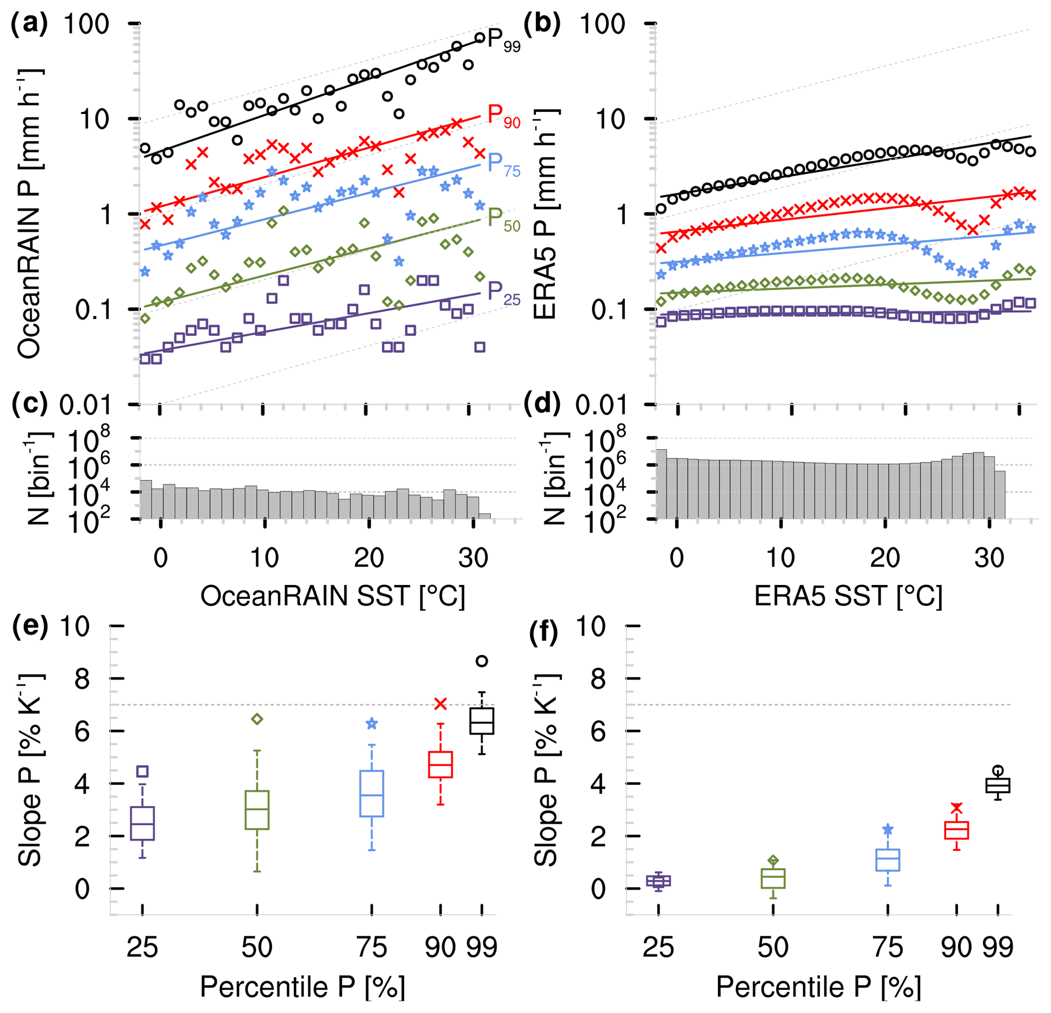
Figure 2 Five percentiles of (a) OceanRAIN (June 2010–April 2017) and (b) ERA5 (June 2010–December 2016) precipitation rate P (mm h⁻¹) as a function of bin-wise SST (^∘C) shown with linear regressions from TSE calculation. Gray lines indicate 7 % K⁻¹ slope. (c, d) Histograms illustrate number of cases N (per bin) for all in (a) and per month in (b). (e, f) Slopes from TSE regressions (% K⁻¹) in (a) and (b) are indicated by markers as a function of percentile. Boxes (5th–95th percentile) refer to the OLS method as a comparison, which uses the halved dataset resampled 100 times.

The interquartile spread of 1 to 2 % K⁻¹ (50 % of the sensitivity) and data samples of much less than 10 000 min for some of the bins (Fig. 2c) indicate a high variability, which is why we put more trust in the sensitivities calculated by the more robust TSE.

Precipitation in ERA5 reveals a local minimum at about 26 ^∘C, which we will discuss later. Altogether, ERA5 shows a much lower P scaling compared to OceanRAIN with values of about 0.3 to 3.1 % K⁻¹ for weak-to-strong and of 4.5 % K⁻¹ for heavy precipitation with TSE (Fig. 2b, f). As these numbers rely on global ocean coverage, even the average monthly data sampling density of 10⁶ per bin (Fig. 2d) strongly exceeds that of OceanRAIN, resulting in a smoother trend of the P scaling and a lower interquartile spread of 0.4 to 0.8 % K⁻¹. As a consequence, the TSE always lies within the uncertainty of the OLS method (5th–95th percentile). Nevertheless, the question arises as to whether only resolution differences cause the systematically lower P scaling in ERA5 compared to OceanRAIN.

3.3 Can vertical velocity help to understand the precipitation scaling with SST?

To enhance our understanding of different P scalings over the ocean, we consider vertical velocity at 500 hPa from ERA5 to select cases that favor precipitation formation. As an indicator, we use the temporal correlation r(P,ω₅₀₀) at each grid point between hourly precipitation (P) and hourly 500 hPa vertical velocity (ω₅₀₀) from ERA5. As in Emori and Brown (2005), we use $r(P,{\mathit{\omega }}_{\mathrm{500}})=-\mathrm{0.2}$ as a threshold (note that we define positive vertical velocity as subsiding motion). The resulting areas of weak or even positive r(P,ω₅₀₀) for a month (bluish colors in Fig. 3a) mainly comprise, but are not limited to, areas of subsidence and relatively low SSTs and amount to 5 % of the global ocean precipitation (see Fig. A1 for influence on ERA5). Unlike earlier studies, note that we use hourly instead of daily (e.g., Emori and Brown, 2005) or monthly time steps (e.g., Oueslati and Bellon, 2015) for correlation, but correlations are calculated per month. The high seasonal variability of r(P,ω₅₀₀) leaves only small areas with a constantly weak r(P,ω₅₀₀) over a whole year (e.g., minimum for each month of 2010 in Fig. 3b). While the size of the areas varies slightly, the southeast Pacific and southeast Atlantic areas of constantly weak correlation stay the same for the years 2010–2016 while elsewhere r(P,ω₅₀₀) remains mostly below −0.2 (not shown).

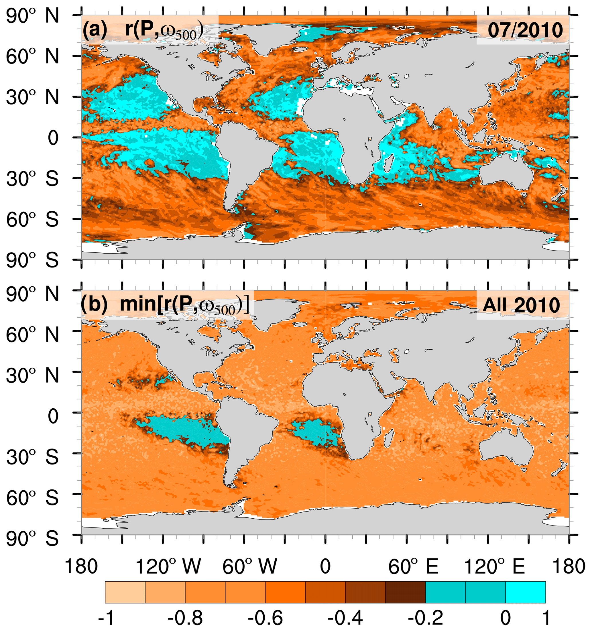
Figure 3 Maps of temporal correlation r(P,ω₅₀₀) for each ERA5 grid box for (a) July 2010 and (b) the minimum monthly correlation for the year 2010. Blue colored areas are weakly or positively correlated and are excluded from further analysis ($r>-\mathrm{0.2}$; Emori and Brown, 2005).

In order to use ω₅₀₀ to constrain OceanRAIN precipitation, we match each minute of OceanRAIN precipitation with the closest hourly ω₅₀₀ of ERA5. Negative ω₅₀₀ values correspond to rising motion. Almost two-thirds of the global-ocean ERA5 time steps during July 2010, as an example, have absolute vertical velocities $\left|{\mathit{\omega }}_{\mathrm{500}}\right|$ below 100 hPa d⁻¹ (Fig. 4a).

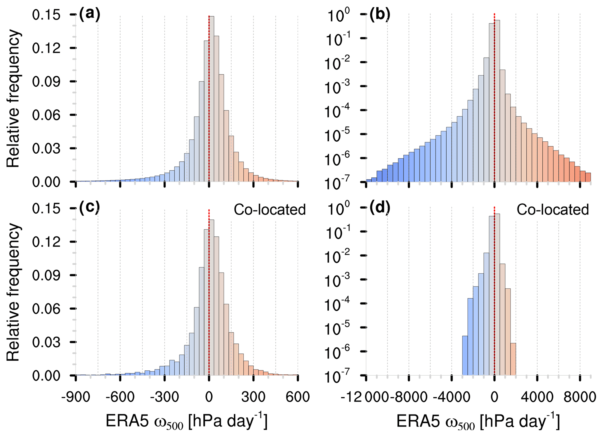
Figure 4 Histograms of relative frequencies for ω₅₀₀ (blue: rising motion; red: subsiding motion) of (a, b) all ERA5 grid boxes and (c, d) for OceanRAIN–ERA5 co-located ERA5 grid boxes with (a, c) linear ordinates and (b, d) logarithmic ordinates for strong motion.

The slightly left-skewed distribution of ω₅₀₀ ($\mathit{\gamma }=-\mathrm{3.44}$) has a 1st percentile of −692 hPa d⁻¹, a 99th percentile of 410 hPa d⁻¹, a mean of −1.1 hPa d⁻¹ and a median of 15.5 hPa d⁻¹ (Fig. 4b). When being matched to OceanRAIN, the ω₅₀₀ distribution of ERA5 loses its extremes (1st percentile, −602 hPa d⁻¹; 99th percentile, 385 hPa d⁻¹; Fig. 4c and d with log y axis) while the left-skewness slightly reduces ($\mathit{\gamma }=-\mathrm{2.03}$). Nevertheless, the ω₅₀₀ distribution of OceanRAIN–ERA5-matched time steps is very similar to the overall ERA5 distribution of July 2010 (Fig. 4a and c).

The OceanRAIN–ERA5-matched time steps enable a direct comparison between both datasets for the P scaling. We define a range of $-\mathrm{1500}<{\mathit{\omega }}_{\mathrm{500}}<-\mathrm{50}$ hPa d⁻¹ that, first, selects upward motion that generally fosters precipitation to form and that, second, provides sufficient matches per SST bin to allow the highest percentiles to be calculated (Fig. 5c, d).

Figure 5 As Fig. 2 but for all OceanRAIN–ERA5-matched time steps for OceanRAIN  (a, c, e) and for ERA5 (b, d, f), both for rising motion ($-\mathrm{1500}<{\mathit{\omega }}_{\mathrm{500}}<-\mathrm{50}$ hPa d⁻¹) and excluding regions of $r(P,{\mathit{\omega }}_{\mathrm{500}})>-\mathrm{0.2}$ from Fig. 3. Orange lines in (c) and (d) mark the lowest N for which P₉₉ can be calculated.

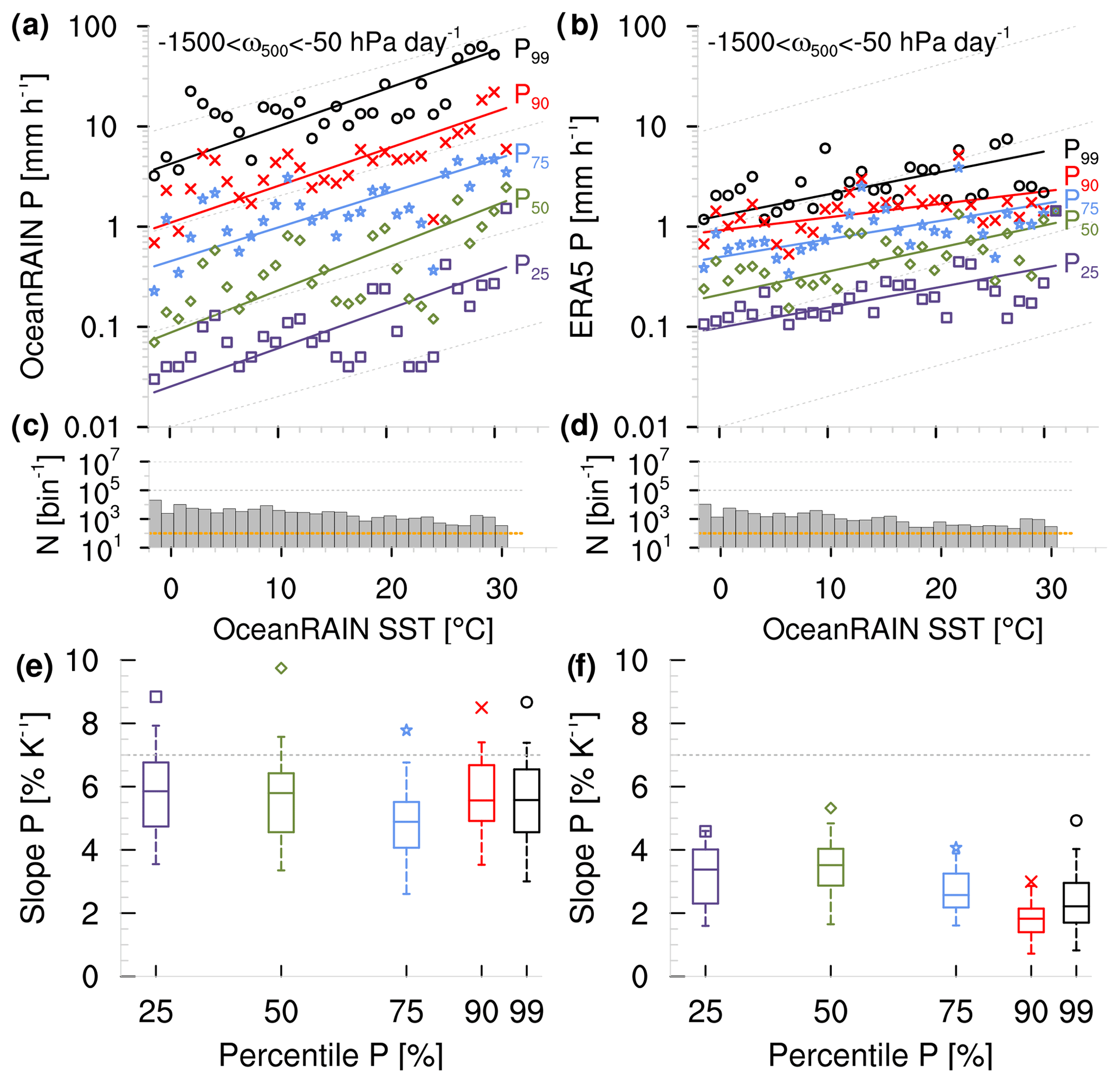
This range represents a good compromise between a clear signal of rising motion and a sufficiently large size of remaining OceanRAIN samples. Third, we exclude grid boxes with a temporal correlation of $r(P,{\mathit{\omega }}_{\mathrm{500}})>-\mathrm{0.2}$ per month that are mainly associated with dry areas of subsidence (see Fig. 3). The influence of these weakly correlated areas on the whole ERA5 dataset is shown in Appendix A (see Fig. A1). Also note that we use OceanRAIN SSTs for both datasets as the usage of ERA5 SSTs would reduce the total number of usable time steps (437 000 without ω₅₀₀ constraint) by 6.6 % (not shown). The resulting subsample of matched time steps for ERA5 (hourly) and OceanRAIN (every minute) comprises about 110 000 time steps. The relatively low number of remaining time steps limits the statistical robustness of the sample for some of the 1 ^∘C SST bins that contain fewer than 1000 precipitation values (Fig. 5c, d). The data sparsity results in a quite scattered sensitivity distribution (Fig. 5a, b). First, compared to the larger sample of OceanRAIN measurements and ERA5 data (see Fig. 2), particularly the weak-to-medium precipitation rates increase at a much higher rate with constrained ω₅₀₀. Second, all OceanRAIN precipitation percentiles scale with 7.5 to 10 % K⁻¹ (ERA5: 3 to 5.5 % K⁻¹) according to TSE (Fig. 5e, f). This means an approximate constant sensitivity of precipitation to a change in SST, for OceanRAIN even at super CC scaling, while the sensitivity difference remains between ERA5 and OceanRAIN.

To understand whether this uniform sensitivity at all precipitation percentiles results from the ω₅₀₀ constraint, from the data sparsity or is a feature of the matched subsample of data, we consider ERA5 with the same constraint of $-\mathrm{1500}<{\mathit{\omega }}_{\mathrm{500}}<-\mathrm{50}$ hPa d⁻¹ but globally for the full ERA5 period, which leads to more than 1000 times more data (monthly N in Fig. 6c).

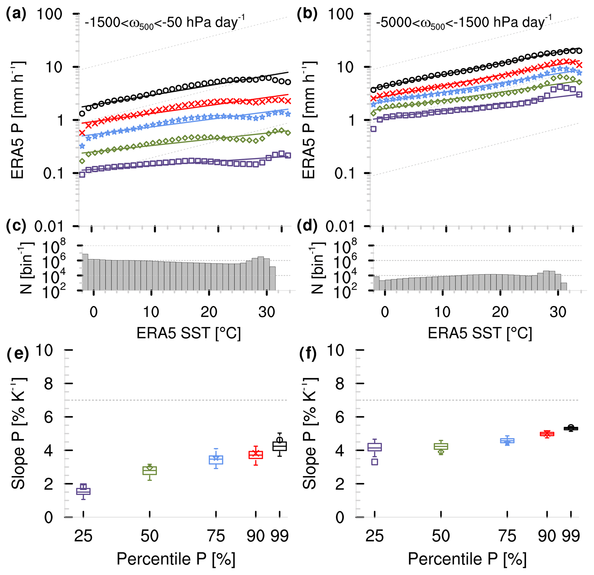
Figure 6 As with Fig. 5 but for the complete ERA5 period. Panels (a), (c) and (e) are constrained by $-\mathrm{1500}<{\mathit{\omega }}_{\mathrm{500}}<-\mathrm{50}$ hPa d⁻¹ and panels (b), (d) and (f) by $-\mathrm{5000}<{\mathit{\omega }}_{\mathrm{500}}<-\mathrm{1500}$ hPa d⁻¹.

Compared to OceanRAIN, the P scaling smoothens for all precipitation percentiles (Fig. 6a) while the interquartile spread reduces (Fig. 6e). Compared to Fig. 5f, mainly the P scaling of weak precipitation decreases below 2 % K⁻¹, and for medium-to-heavy precipitation it remains between 3 and 5 % K⁻¹. Compared to Fig. 2e, the P scaling increases more steeply for weak precipitation and reaches a plateau for medium-to-strong intensities before it increases again for heavy precipitation. Accordingly, the sensitivity in Fig. 5f points at the slightly increased sensitivities for low precipitation rates for the ω₅₀₀ constraint while the picture is mainly blurred due to the small sample size.

Constraining ω₅₀₀ to rising motion strongly reduces the local minimum at about 26 ^∘C in Fig. 2b (see Fig. 6a). From this and areas of weak or positive correlation between SST and precipitation (Figs. 3 and A1), we suppose that atmospheric conditions of weak ω₅₀₀ contribute to the local minimum at 26 ^∘C in ERA5. It might therefore seem natural that suppressed dynamical drivers of precipitation, predominantly in the subtropics, could generate this local minimum in precipitation intensity. Proving this assumption, however, goes beyond the scope of this work.

To further investigate the influence of a constraining ω₅₀₀, we consider stronger rising motion between −5000 and −1500 hPa d⁻¹ (Fig. 6b). Compared to somewhat weaker rising motion in ω₅₀₀, the weak precipitation rates increase by about 1 order of magnitude, while heavy precipitation rates are higher by a factor of 2. The change in the P scaling with SST smoothens while it tends towards a constant slope at all percentiles (Fig. 6f). This constant slope marks a linear increase and saturates for strongest rising motions at approximately 6 % K⁻¹ in ERA5 (not shown). Accordingly, the shift of the range of ω₅₀₀ toward lower values (rising motion) tends to equalize the P scaling at different P percentiles. This mainly results from an increase in P scaling at lower percentiles, while the P scaling remains approximately constant for high percentiles.

3.4 Does a change in precipitation event duration with SST affect the precipitation scaling?

Over land, previous studies state a decrease in precipitation event duration with increasing air temperature that explains the drop-off in precipitation scaling at high temperatures found for hourly to daily sampling rates (Haerter et al., 2010; Utsumi et al., 2011). Haerter and Berg (2009) explain the decreasing event duration with a shift toward more convective precipitation events at high temperatures. To check whether this holds over the ocean, we calculated the OceanRAIN precipitation event duration by counting uninterrupted periods of continuous precipitation at 1 min sampling. The average precipitation event lasts between 6 and 11 min with an uncertainty of 1 to 2 min obtained from bootstrapping (Fig. 7a).

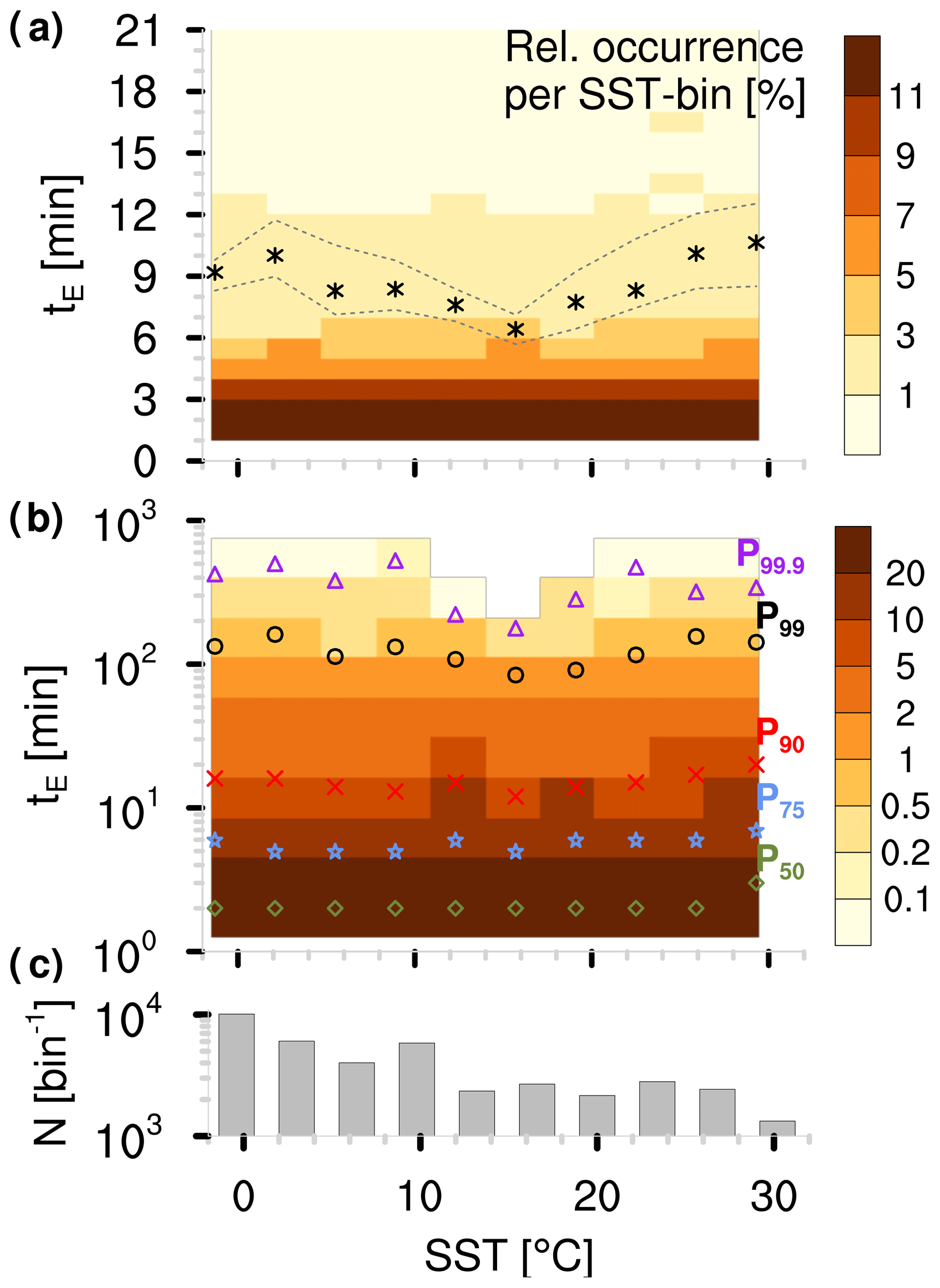
Figure 7 Two-dimensional histograms as a function of precipitation event duration t_E (min) and OceanRAIN SST (^∘C) for (a) linear and (b) logarithmic ordinate. Colors indicate relative occurrence (%) per SST bin. Markers in (a) show mean per SST bin surrounded by minimum and maximum from resampling 100 times as a measure of uncertainty. Markers in (b) show percentiles 50, 75, 90, 99 and 99.9 of t_E. Panel (c) shows the number N of events per SST bin.

The shortest mean precipitation event duration occurs at 15 ^∘C, while the longest mean precipitation event duration occurs around 2 ^∘C and above 28 ^∘C. The mean is mainly driven by the highest percentiles (99th to 99.9th exceeding 2 h) that mainly cause the minimum at 15 ^∘C, but it is less pronounced for the 50th to 75th percentile where precipitation event duration remains constant (Fig. 7b). Although the precipitation event duration tends to decrease between 2 and 16 ^∘C as over land (Haerter et al., 2010; Utsumi et al., 2011), we find no systematic decrease over the whole SST range.

The precipitation event duration as a function of temperature can be influenced by several factors. First, the heterogeneous sampling in OceanRAIN can influence the event duration. Exceeding 2000 samples per bin, the sampling density per SST bin seems fairly good for most of the SST range; below 12 ^∘C it even exceeds 4000 samples per bin (Fig. 7c). Nevertheless, heterogeneous spatial sampling by the ships can lead to a biased picture (see Fig. 3 in Burdanowitz et al., 2018); e.g., the eastern Atlantic has been more densely sampled compared to the western Atlantic, which might have an effect on the occurrence of very long-lasting precipitation events. Second, the ship movement relative to cloud movement can affect the retrieved event duration. However, this effect cancels out over almost 40 000 events sampled from OceanRAIN (not shown). Overall, influences by the heterogeneity of OceanRAIN on the precipitation event duration cannot be ruled out but seem rather limited according to our investigations.

4 Summary and concluding remarks

This study forms the oceanic counterpart to numerous observational studies over land concerning the sensitivity of extreme precipitation to a change in air temperature. Unlike earlier studies with mainly hourly to daily sampling calling for higher resolution (e.g., Panthou et al., 2014; Drobinski et al., 2016), we consider precipitation rate and SST at a very high sampling rate of 1 min from OceanRAIN optical disdrometer measurements aboard global-ocean research vessels. In addition, hourly measurements of the new ERA5 reanalysis serve to compare and, additionally, constrain precipitation by large-scale vertical velocity.

OceanRAIN challenges the user with its non-uniform sampling and variable spatial resolution along ship tracks. However, at the same time, it offers a unique opportunity to study oceanic precipitation at high quality with global-ocean sampling at 1 min temporal resolution. Additionally, we show that differences in seasonal and latitudinal sampling are small, which could otherwise affect the precipitation scaling (Schroeer and Kirchengast, 2018). Furthermore, the OceanRAIN average precipitation distribution with latitude looks similar to that in ERA5 with its homogeneous global-ocean coverage.

For OceanRAIN, the 99th percentile of 1 min precipitation rates shows a super CC scaling of almost 9 % K⁻¹ in line with studies over land (e.g., Bürger et al., 2014; Schroeer and Kirchengast, 2018), while for ERA5 the 99th percentile of the hourly ERA5 precipitation rates increases by only 4.5 % K⁻¹ (linear regression using Theil–Sen estimator). The tendency of a stronger scaling with higher temporal sampling confirms findings by Utsumi et al. (2011) and Drobinski et al. (2016). This difference in CC scaling ranges between 4 and 6 % K⁻¹ for the weak-to-strong precipitation rates between OceanRAIN and ERA5. For both datasets, precipitation increases with SST at all the percentiles considered. In contrast to studies over land, we find no “hook shape” (Drobinski et al., 2016) or clear drop-off (Hardwick Jones et al., 2010) of precipitation over the ocean towards high SSTs. Drobinski et al. (2016) explain the “hook shape” by the lifted level of condensation under higher surface temperatures in a dry environment. Instead, despite the variability in OceanRAIN, we find a continuous increase in OceanRAIN precipitation with increasing SST, including the highest SSTs.

Nevertheless, the ERA5 precipitation rates reveal a local minimum at about 26 ^∘C. When excluding areas of weak temporal correlation of 500 hPa vertical velocity with precipitation rate, the local minimum in precipitation scaling becomes weaker. Despite the fact that the hourly vertical velocity might not necessarily be the best indicator of large-scale subsidence, the minimum vanishes when constraining precipitation to rising motion below −1500 hPa d⁻¹. From this, we infer that dynamical drivers such as subtropical large-scale subsidence inhibit precipitation formation and cause the local precipitation minimum at 26 ^∘C. However, it remains open whether this minimum reveals a deficiency in ERA5 – e.g., by suppressing precipitation formation too strongly in the subtropics – or whether this minimum has not yet become visible in OceanRAIN due to limited sampling.

The data sampling density plays a crucial role in precipitation-sparse regions that would need the longest sampling to be well represented. Generally, the non-uniform sampling by ships in OceanRAIN results in a more variable precipitation distribution with respect to SST. Therefore, we mainly rely on the Theil–Sen estimator (TSE) as linear regression method, which is less susceptible to outliers (Wilcox, 2001), instead of only trusting the widely known ordinary least squares (OLS) method.

Although we find a more steady precipitation scaling in OceanRAIN compared to ERA5 at high SSTs, there is no evidence that this is caused by a decreasing duration of precipitation events with temperature as indicated by studies over land (Haerter et al., 2010; Utsumi et al., 2011). Instead, we find a minimum average precipitation event duration in OceanRAIN of 7 min at about 15 ^∘C that rises beyond 10 min above 28 ^∘C. This temperature dependence remains the same for higher percentiles corresponding to longer events. As most of the precipitation events last only a few minutes, this confirms our decision to use a high-temporal-sampling rate of 1 min to exclude resolution artifacts from the precipitation scaling. At 1 min resolution, we find no evidence of generally decreasing precipitation event duration with temperature.

For the OceanRAIN–ERA5-matched time steps, we find a high uncertainty for the reduced data sample using vertical velocity in 500 hPa from ERA5 to constrain precipitation rates. The OceanRAIN precipitation scales with super CC behavior at all precipitation percentiles (8 to 10 % K⁻¹) while ERA5 precipitation scales with 3 to 6 % K⁻¹, confirming the offset that we found between both unconstrained datasets. The offset in precipitation scaling is therefore likely attributable to the marked difference in spatial resolution that confronts the OceanRAIN along-track data with the areal ERA5 data of 31 km grid boxes. Furthermore, constraining precipitation towards strongly rising air masses leads to a precipitation scaling that converges towards 6 % K⁻¹ for all precipitation rates in ERA5. For OceanRAIN, the too small data sample for precipitation in lifting air masses does not allow us to derive a number for the scaling, but the offset to ERA5 and the scaling with the OceanRAIN–ERA5-matched data both suggest super CC scaling for OceanRAIN.

Two aspects should be kept in mind when interpreting our results. First, the average precipitation scaling should not be directly translated into an increase in local precipitation per degree of warming, as locally dynamic processes can strongly alter the precipitation–SST relationship. Second, in light of the projected rising global mean temperature by anthropogenic climate change, large-scale circulation changes and other side effects in the Earth system could contribute or counteract the diagnosed precipitation sensitivity to a change in SST. Therefore, care needs to be taken when interpreting our results that are valid under the present climatic conditions.

The next steps would include more local analyses at 1 min resolutions once data sampling allows the highest precipitation intensities to be resolved globally. Furthermore, higher resolutions are needed in global climate models to project the hydrological sensitivity of extremes in a warming climate and its feedbacks.

Appendix A: How circulation dynamics impact the precipitation scaling in ERA5

Figure A1 Panels (a), (c) and (e) are the same as right panel of Fig. 2. Panels (b), (d) and (f) exclude regions of $r(P,{\mathit{\omega }}_{\mathrm{500}})>-\mathrm{0.2}$ from Fig. 3 for the complete ERA5 period.

To shed light on the influence of circulation dynamics on the P scaling of ERA5, we consider the temporal correlation r(P,ω₅₀₀). According to Emori and Brown (2005), we exclude all precipitation time steps with $r>-\mathrm{0.2}$ diminishing the influence of precipitation from very shallow convection and large-scale subsidence. The resulting precipitation distribution with respect to SST reveals a less pronounced minimum at about 26 ^∘C (Fig. A1b).

This leads to a slight increase in the P scaling at all intensities (Fig. A1e–f). Accordingly, ω₅₀₀ itself can better explain the minimum at 26 ^∘C compared to areas of low correlation between ω₅₀₀ and P.