the Creative Commons Attribution 4.0 License.
the Creative Commons Attribution 4.0 License.
 | 17 Jul 2019
Elucidating ice formation pathways in the aerosol–climate model ECHAM6-HAM2
Remo Dietlicher
David Neubauer
Ulrike Lohmann
Cloud microphysics schemes in global climate models have long suffered from a lack of reliable satellite observations of cloud ice. At the same time there is a broad consensus that the correct simulation of cloud phase is imperative for a reliable assessment of Earth's climate sensitivity. At the core of this problem is understanding the causes for the inter-model spread of the predicted cloud phase partitioning. This work introduces a new method to build a sound cause-and-effect relation between the microphysical parameterizations employed in our model and the resulting cloud field by analysing ice formation pathways. We find that freezing processes in supercooled liquid clouds only dominate ice formation in roughly 6 % of the simulated clouds, a small fraction compared to roughly 63 % of the clouds governed by freezing in the cirrus temperature regime below −35 ∘C. This pathway analysis further reveals that even in the mixed-phase temperature regime between −35 and 0 ∘C, the dominant source of ice is the sedimentation of ice crystals that originated in the cirrus regime. The simulated fraction of ice cloud to total cloud amount in our model is lower than that reported by the CALIPSO-GOCCP satellite product. This is most likely caused by structural differences of the cloud and aerosol fields in our model rather than the microphysical parametrizations employed.
- Article
(6274 KB) - Full-text XML
- BibTeX
- EndNote


Clouds are an important modulator for Earth's climate. They exert a net radiative effect of approximately −20 W m−2 and thus significantly cool the planet (Boucher et al., 2013). Compared to this, the forcing induced by well-mixed greenhouse gases since pre-industrial times is almost 1 order of magnitude smaller, approximately 3 W m−2 (Myhre et al., 2013), and has the opposite sign associated with a warming. Small changes in the cloud radiative effect can therefore easily offset or strengthen a greenhouse-gas-induced warming. In fact, there is a broad consensus that clouds contribute the largest uncertainty for climate projections in state-of-the-art atmospheric general circulation and Earth system models (Flato et al., 2013).
The models that contributed to the Coupled Model Intercomparison Project Phase 5 (CMIP5) generally agree that cloud adjustments to a warming climate will likely further reinforce the initial warming, a positive feedback loop. Clouds are expected to become fewer, higher and optically thicker in the global mean (Zelinka et al., 2013).
The warming response of cloud ice has been hypothesized to counteract and therefore reduce the global mean, net positive cloud feedback through a transition from optically thin ice clouds in the present-day climate to optically thick liquid clouds in a warmer climate (Mitchell et al., 1989; Storelvmo et al., 2015; Ceppi et al., 2016; Frey and Kay, 2018). The magnitude of this so-called cloud phase feedback strongly depends on the simulation of the present-day cloud phase partitioning in models. It is well established that models tend to underestimate the ratio of supercooled liquid water to ice in present-day conditions (Cesana et al., 2015). This leads to an overestimation of the magnitude of the cloud phase feedback (Li and Le Treut, 1992; Terai et al., 2016; Tan et al., 2016) in a greenhouse-gas-induced, warmer climate in some models. Recent modelling efforts challenge the universality of this finding (Lohmann and Neubauer, 2018; Bodas-Salcedo, 2018), calling for a more comprehensive description of ice formation pathways in general circulation models (GCMs).
Especially sensitive to global warming is ice in mixed-phase clouds, predominantly originating from heterogeneous immersion or contact freezing of mineral dust (Atkinson et al., 2013; DeMott et al., 2015; Kanji et al., 2017). Those clouds are usually found in the temperature range between −38 and 0 ∘C, which we therefore refer to as the mixed-phase temperature regime. Beyond the theoretical and experimental uncertainties of the freezing mechanisms (Welti et al., 2014; Ickes et al., 2015; Marcolli, 2017), a realistic representation of cloud glaciation is further complicated by uncertainties in the parameterization of subsequent ice growth and sedimentation. Due to the lower saturation water vapour pressure over an ice crystal compared to a liquid droplet surface, cloud ice can grow below water saturation, eventually leading to evaporation of the cloud droplets. This process is called the Wegener–Bergeron–Findeisen (WBF) process and can glaciate a cloud within minutes to hours (Korolev and Isaac, 2003), depending on the number of ice crystals, temperature and vertical velocity of the air parcel.
Due to the complex processes governing mixed-phase clouds, models inhibit a very large spread in the simulation of the phase partitioning (Fan et al., 2011; McCoy et al., 2016). A model intercomparison study of Komurcu et al. (2014) found for the six models (ECHAM6, CAM-IMPACT, CAM-Oslo, CAM5.1 MAM3, CAM5.1 MAM7, SPRINTARS) in their study that even for the same ice nucleation parameterizations, the spread in the simulated phase partitioning among the models was not reduced.
A significant portion of cloud ice is found at temperatures below −38 ∘C. There, ice crystals can freeze homogeneously from pre-activated cloud droplets (Lohmann et al., 2016) and deliquesced aerosols (Koop et al., 2000) or nucleate directly on an ice nucleating particle (INP). The latter two processes do not require water saturation, leading to fundamentally different types of cirrus clouds (Krämer et al., 2016; Wernli et al., 2016; Gasparini et al., 2018) with significant differences in the respective microphysical and thus optical properties, highlighting the need for a correct representation of ice formation pathways of all clouds containing ice, not just those in the mixed-phase regime.
These complex, sub-grid-scale processes can only be studies through idealized laboratory measurements and inferred from comprehensive field studies which are usually conducted over small areas. Being weakly constrained, ice process parameterizations differ greatly among models and because of that different ice formation pathways can be favoured, leading to the wide spread in phase partitioning among models (Cesana et al., 2015; McCoy et al., 2016). To find the parameterizations that control the cloud phase partitioning, we need to quantify the impact each process has on the simulated cloud fields.
The amount of ice that forms following a nucleation event in either a mixed-phase or cirrus cloud strongly depends on the available humidity and, in the case of mixed-phase clouds, liquid water. A strong nucleation event does not necessarily induce a long-lived or massive ice cloud and vice versa. Furthermore, sedimentation of cloud ice disconnects ice initiation and growth regions, which further complicates diagnosis of the causal link between the parameterized microphysical processes and the observed cloud state. Traditional, spatio-temporally averaged model output usually reports the mean state of the cloud fields and sometimes microphysical tendencies, but does not allow the dominant microphysical formation mechanisms to be traced back due to the reasons above. Unlike the real atmosphere, which does not directly reveal its governing processes, the models do so by definition. Here we harvest this additional information that is present in the models by introducing additional tracers to quantify the microphysical ice formation pathways along with the model integration to assess the importance of different ice initiation and growth mechanisms.
Furthermore, we use the pathway analysis to classify clouds and accumulate statistics on their properties. The benefit of cloud classification is well established and has a long history. A common method is the identification of dynamical cloud regimes to compute conditional statistics (Jakob and Tselioudis, 2003; Williams and Tselioudis, 2007; Williams and Webb, 2009; Tsushima et al., 2016). These methods use high-frequency output and short-term temporal aggregation of cloud top temperature vs. cloud optical thickness histograms together with clustering algorithms, classifying the mean dynamic states over the aggregation period. Our method focuses on the microphysics of cloud formation linking parameterizations and the resulting cloud fields. This link is essential to identify the parametrizations responsible for potential model-to-model or model-to-observation mismatches.
This study is based on an adapted version of the predicted bulk particle properties (P3) scheme of Morrison and Milbrandt (2015) for the use in a GCM. Single-category ice phase microphysics schemes have recently also been implemented in the Community Atmosphere Model Version 5 (CAM5) GCM (Eidhammer et al., 2017; Xi et al., 2017). Dietlicher et al. (2018) (hereafter D18) provides a detailed description of the technical aspects of the implementation of P3 in ECHAM6-HAM2, the GCM we use in this study. This scheme has the decisive advantage of representing cloud ice in a consistent manner, predicting the particle size distribution as well as the mass-to-size relationship. It employs one single, prognostic ice phase category, rendering heuristic conversion rates between in-cloud and precipitation type ice hydrometeors unnecessary. Process rates are computed offline and read back from look-up tables. This allows each process rate to be integrated over the entire particle spectrum. For example, our scheme consistently represents the size dependence of the depositional growth rate using a size-dependent ice crystal capacitance. Simplified, size-independent ice crystal growth rates are hypothesized to significantly contribute to the large spread among models in the simulated phase partitioning (Fan et al., 2011).
This study can be divided into two parts. First, we show how the new model performs on the global scale and then introduce the method to elucidate the ice formation pathways in the second part of this study. In Sect. 2 we highlight the main differences in our model compared to the reference model version ECHAM6.3-HAM2.3 and discuss the new cloud fraction parameterization that has been added since the previous description of the version in D18. We evaluate the simulation of clouds, with a special focus on cloud ice, against a series of satellite observations in Sect. 3. In the second part, we introduce additional prognostic equations that are solved to quantify ice formation pathways in Sect. 4. In Sect. 5 we compile a climatology of cloud types based on these ice formation pathways and demonstrate how they can help us understand cloud phase partitioning.
The improvements to the previous model version (ECHAM6.3-HAM2.3; Neubauer et al., 2014) (hereafter called the reference model) are twofold. In the new model, cloud ice is a fully prognostic quantity, i.e. the advection equation for vertical transport (sedimentation) is solved online. Describing all ice particles with only a single category based on Morrison and Milbrandt (2015) no longer requires the heuristic partitioning between in-cloud ice and precipitating snow. The technical details of the model regarding prognostic treatment of sedimentation and the associated numerical stability restrictions on the time step as well as an inter-comparison of the different ice representation schemes can be found in D18. Here we will focus on the global evaluation of the new model both in terms of the feasibility of the results as well as computational performance.
The (P3) scheme presented in Morrison and Milbrandt (2015) predicts four properties of the ice particle distribution: the total ice mass mixing ratio qi, the total ice number mixing ratio Ni, the rimed ice mass mixing ratio qrim and the rimed ice density brim. Originally developed for the Weather Research and Forecasting model (WRF), the scheme was not intended for the coarse resolution of GCMs and climate projections. As we have shown in D18 by idealized single-column model (SCM) simulations, GCMs are likely unable to properly represent small-scale weather features like squall lines to produce significant rimed ice formation. We test this hypothesis in the global set-up of ECHAM-HAM in this paper.
The single conceptual deviation from the microphysics scheme described in D18 concerns the sub-grid cloud cover parameterization. While this work focuses on the importance of the representation of cloud ice, the sub-grid cloudiness is a fundamental property of clouds in GCMs, governing both cloud–radiation and cloud–precipitation interactions.
The approach taken in D18 tried to minimize the difference between the new and the reference model by extending the approach of Sundqvist et al. (1989) (hereafter S89) to ice clouds with a smooth transition from liquid water to ice clouds. As we will discuss in Sect. 3, this scheme leads to a strong positive bias of cloud cover for cirrus clouds. Therefore, we used a slightly different cloud cover scheme here.
The cloud cover scheme has also implications for the growth by condensation and deposition. Diagnosing sub-grid cloud cover from the large-scale relative humidity creates a tight link between the cloud fraction and growth by condensation or deposition. The fundamental concept of the S89 scheme is that convergence of humidity within a grid box contributes to an increase in total cloud water by condensation and deposition as well as an increase in the cloud fraction through moistening of the grid box. Here we extend this idea to cold clouds and implement a cloud cover scheme which treats the microphysical structure of ice clouds consistently, requiring mixed-phase clouds to form via the liquid phase and allowing supersaturation in the cirrus regime.
2.1 Sub-grid cloud fraction
The original sub-grid cloud cover scheme of S89 does not consider cloud ice and assumes that a grid box will be fully covered by the cloud if the water vapour mixing ratio qv surpasses the liquid water saturation mixing ratio qsw, i.e. the relative humidity with respect to liquid water sw satisfies . Cloud cover b increases with increasing sw as follows:
The parameter smin is the threshold relative humidity for sub-grid cloudiness below grid box mean water saturation and . The assumptions underlying Eq. (1) are reasonable for synoptic-scale warm clouds. However, this scheme cannot be easily extended to cold clouds where a grid box may or may not contain cloud ice in the mixed-phase regime, rendering the global use of sw for all temperatures inadequate. At the same time, relative humidity with respect to ice (si) can reach values higher than 140 % before ice nucleates from deliquesced aerosols (Koop et al., 2000), which is inconsistent with the use of for ice clouds at cold temperatures. A few approaches exist to overcome either of these aspects. In the following we present the reasoning that led to the development of the new method used here. For an overview, see Fig. 1.
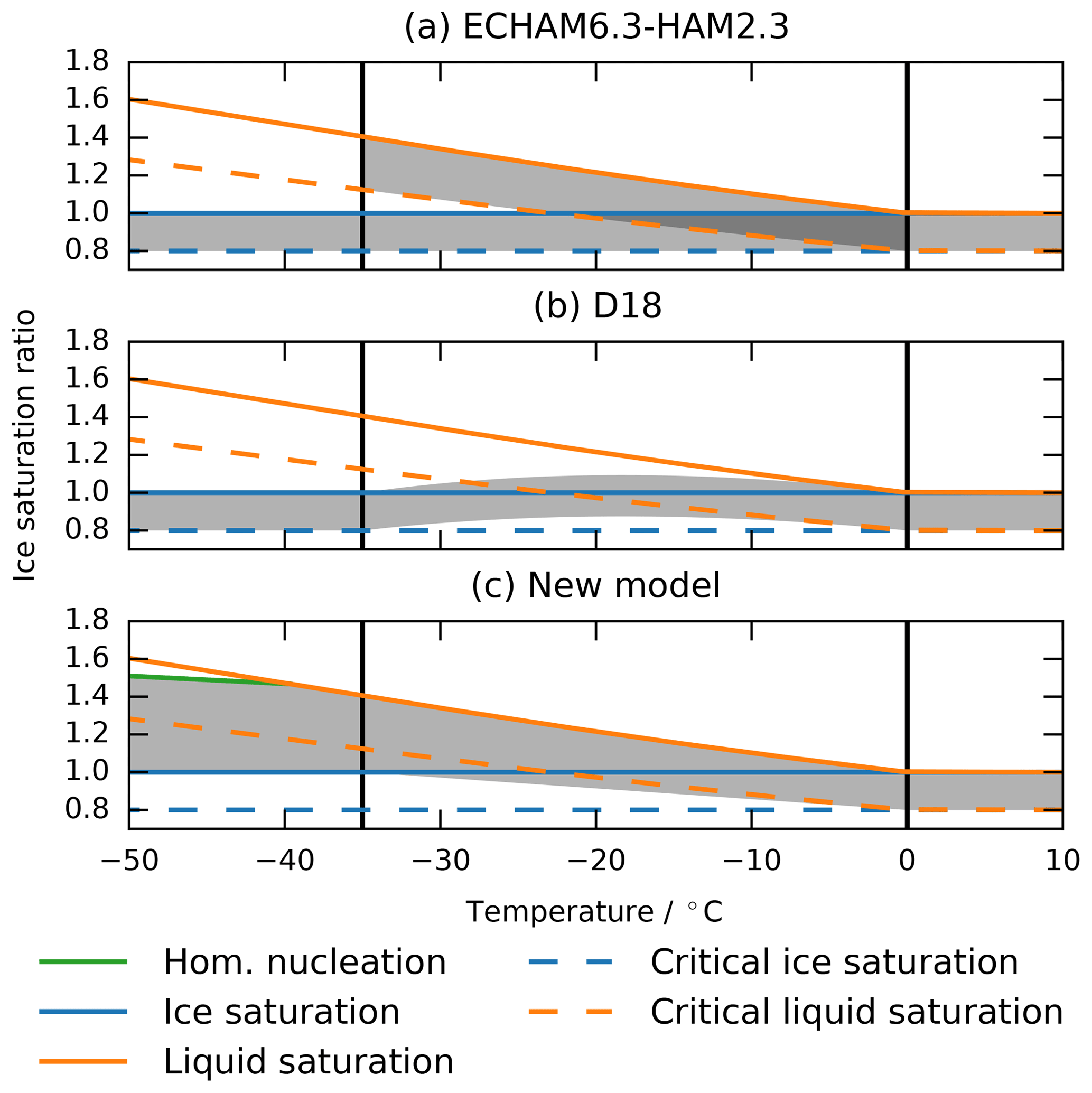
Figure 1Regions where clouds can form (grey shaded areas) as a function of temperature and supersaturation with respect to ice. The coloured lines show liquid water and ice saturation ratios sw∕i (solid lines) and the critical saturation ratios required for first cloud formation (dashed; sw∕iK). We choose a constant K=0.8 for this illustration. Panel (a) shows the sub-grid cloud scheme of the reference model ECHAM6.3-HAM2.3 which switches between liquid and ice saturation in the mixed-phase regime, (b) shows the mixed-saturation approach of Dietlicher et al. (2018) (D18) and (c) shows the new model.
As illustrated in Fig. 1a, Lohmann and Roeckner (1996) (the method used in the reference model) replaced sw in Eq. (1) by si if a threshold amount of ice is exceeded within the grid box. This approach has the drawback that clouds artificially expand upon glaciation because of the lower saturation water vapour pressure over ice than over liquid water. A similar approach is taken in Morrison and Gettelman (2008) (and D18; illustrated in Fig. 1b) where instead of the discontinuous transition from liquid water to ice saturation, the saturation liquid and ice water vapour mixing ratios are interpolated between qsw and qsi as a function of temperature in the mixed-phase regime. The drawback here is that this interpolated value is not directly relatable to a physical quantity as it does not arise from a valid solution of the Clausius–Clapeyron equation. Both of these schemes are not designed to allow for sub-grid clouds in the cirrus regime where si needs to be well above 1 for ice nucleation to occur; i.e. all cirrus clouds formed by homogeneous freezing will occupy the entire grid box. Supersaturation with respect to cloud ice has been accounted for in the cloud cover scheme by Gettelman et al. (2010), where individual cloud fractions for liquid water and ice clouds are computed with a functional dependency of the cloud fraction b(s) similar to Eq. (1) but relaxing the relative humidity for complete cloud coverage to for ice clouds and treating the value of smax as a model parameter.
The cloud fraction parameterization used in our microphysics scheme is very similar to this last approach, but we do not separate cloud cover for liquid and ice clouds. After all, in the mixed-phase regime we expect ice clouds to originate from liquid clouds (Ansmann et al., 2009; Hoose et al., 2010; Hande and Hoose, 2017). Furthermore, the magnitude of supersaturation for complete cloud cover in Gettelman et al. (2010) is arbitrary. The scheme presented here uses a limit which is consistent with the parameterization of ice nucleation based on the theory of Koop et al. (2000). This scheme is illustrated in Fig. 1c.
One can associate smin and smax in Eq. (1) with the minimal relative humidity below which clouds start to evaporate and the maximal relative humidity which can be reached before the cloud covers the entire grid box. These two constraints provide some guidelines on how to extend the S89 scheme to cold clouds.
For clouds that form via liquid water, we assume that smax is reached at liquid water saturation, e.g. when liquid water is assumed to condense immediately, which is a reasonable assumption for stratiform clouds. At temperatures warmer than −35 ∘C, any ice must form via liquid water, consistent with the above-mentioned lidar observations and modelling studies. For colder temperatures, it has been shown (Koop et al., 2000) that ice can nucleate from deliquesced aerosols already below liquid water saturation.
The minimal relative humidity smin must be chosen such that ice does not sublimate above ice saturation. Cloud ice can sediment into and form within the mixed-phase regime. For this reason, and in order to retain sub-grid cloudiness for warm clouds, must hold for all temperatures.
2.2 Growth by condensation and deposition
The water vapour available for condensation is linked to the cloud cover b by the following:
where Δqv is the moisture convergence in the grid box by the resolved transport and Δqsw is the change in liquid water saturation water vapour mixing ratio according to the Clausius–Clapeyron equation. Growth by deposition A is computed as a function of the relative humidity with respect to ice si (see e.g. D18):
where αm=0.5 is the probability of a water vapour molecule to successfully be incorporated into an ice crystal, Δt is the model time step and C is the mean ice particle capacitance integrated over the particle size distribution. The parameters and are thermodynamic parameters depending only on temperature.
The maximal amount of water that can deposit in a single time step is given by the following:
where ql is the liquid water mixing ratio and qsi is the saturation water vapour mixing ratio with respect to ice. Equation (4) implicitly represents the WBF process in mixed-phase clouds through the inclusion of ql. The last term in Eq. (4) allows any water vapour which is supersaturated with respect to cloud ice to deposit onto ice crystals and thus requires to add qi to the water vapour mixing ratio for the computation of the relative humidity in Eq. (1) to prevent clouds from shrinking due to deposition. To account for ice clouds, we replace the relative humidity with respect to liquid water sw in Eq. (1) by the more general relative humidity term s defined below.
Combining the considerations for growth by condensation/deposition and the computation of cloud fraction, we obtain the key parameters for the computation of sub-grid cloudiness in Table 1. Two new parameters are introduced: the critical relative humidity with respect to liquid water for warm clouds K, which is equivalent to the parameterization for warm clouds used in the reference model and based on Xu and Krueger (1991), and the relative humidity required for nucleation of ice from deliquesced aerosols skoop according to the activation theory of Koop et al. (2000) in the cirrus regime.
Table 1The parameters involved in the cloud cover scheme, Eqs. (1) and (4). The rows show different parameters as a function of the temperature regime T. We discuss two different choices for s and Qi in the text, and s2/Qi,2. We use a linear weighting function for T in K.
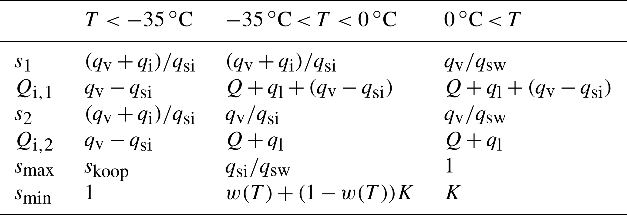
Two versions of the s and Qi terms are given in Table 1 and represent two different methods to treat depositional growth in the mixed-phase regime. They bracket the main problem associated with cloud ice when diagnosing cloud cover from relative humidity. Cloud ice should be able to grow as long as water vapour is supersaturated with respect to ice. Since we are using the relative humidity with respect to liquid water (which is lower than the relative humidity with respect to ice) as maximal relative humidity smax in the mixed-phase regime, ice growth below water saturation leads to a decrease in relative humidity and therefore lowers the cloud fraction b. Therefore we implement two versions of the new scheme. The first, default, method (denoted by a subscripted 1) links cloud cover to the ice mass mixing ratio. It allows cloud ice to grow below liquid water saturation and adds cloud ice to water vapour for the computation of s in Eq. (1) to avoid cloud shrinking by vapour deposition. However, this coupling makes the sedimentation sink of cloud ice also a sink for cloud fraction. We test the sensitivity of this coupling with a second method (denoted by a subscripted 2) where ice growth is inhibited below water saturation in the mixed-phase regime.
We evaluate the new model against a series of satellite observations as well as the reference model and test sensitivities to parametrization choices. Namely, we extend the investigation of ice properties presented in D18 to the global set-up of ECHAM-HAM and assess the behaviour of the new cloud cover parametrization. Furthermore, we use an updated version of the cirrus parametrization, including heterogeneous ice nucleation of mineral dust at temperatures below −35 ∘C at low ice supersaturation based on Kärcher et al. (2006) (implementation courtesy of Steffen Münch, personal communication, 2018).
Results from five different model configurations for 10 years from 2003 to 2012 are shown, one with the reference model (ECHAM6.3-HAM2.3; REF) and four with the new scheme. We assess the influence of rime properties in the full P3 scheme (4M) by comparison with a model configuration where the rime properties are set to zero () (2M). For the reasons presented below, we use the latter as the default configuration of the new model. With 2M as the starting configuration, we then investigate the effect of the artificial sedimentation–cloud-cover feedback introduced by the new cloud cover scheme by limiting ice growth to liquid water saturation (LIM_ICE) and use an updated version of the cirrus cloud parametrization which includes heterogeneous ice nucleation on mineral dust below −35 ∘C (HET_CIR). The simulations and the employed tuning parameters are summarized in Table 2. The tuning parameters have been adjusted such that the model is in radiative balance at the top of the atmosphere (TOA) for the simulations 2M, HET_CIR and REF.
Table 2Description of the model configurations shown in this paper. Tuning parameters are as follows: γr is the scaling factor for warm rain formation, ffall is a scaling factor for ice sedimentation speed, γs is a scaling parameter for snow formation, eii is the collision efficiency of ice crystals, and γcpr is the conversion rate from cloud water and ice to precipitation in the convection scheme. Dashes (–) denote that those parameters are no longer needed in the new scheme. The last column shows the CPU time for 1 year of simulation relative to the reference model.

3.1 Computational performance
The new model employs an adaptive time-stepping scheme to achieve numerical stability for the solution of the vertical advection equation for prognostic sedimentation of cloud ice. Sub-stepping the microphysics scheme comes at a cost, quantified by the CPU time column in Table 2. The numbers shown are computed from 1 year of simulation. Numbers vary by a few percent between runs, illustrated by the differences between the 2M, LIM_ICE and HET_CIR simulations, which are comparable in terms of model complexity. Compared to the reference model, the new model runs approximately 25 % slower in the 2M/LIM_ICE/HET_CIR set-ups and 40 % slower in the 4M set-up. This difference is mainly due to the high fall speeds of rimed particles in the 4M simulation, which require more sub-steps. Compared to this, the cost of advecting two additional tracers is small.
3.2 Comparison to the reference model
Two main differences between the new model and the reference model are immediately evident from Table 2. The single category no longer requires heuristic parametrizations for falling ice crystals and snow formation. At the same time, the new cloud cover parametrization allows the scaling factors to be reduced, effectively bringing the parametrizations closer to their conceptual origin.
To illustrate the most prominent differences in the simulated cloud field, we compare cloud water contents (ice and liquid) as well as cloud cover in Fig. 2 of the new model in the 2M configuration to the reference model. It is evident that the new model produces a lot more ice than the reference model. A large part of the difference can be explained by the fact that the single-category scheme includes cloud ice and snow while snow is a diagnostic quantity which is not included in the ice water content in the two-category scheme employed in the reference model. Of course there are other contributing factors like parameter tuning, a switch from the parametrization of homogeneous freezing of cloud droplets from Kärcher and Lohmann (2002) to Jeffery and Austin (1997) for technical reasons and the cloud cover parametrization, which are hard to disentangle.
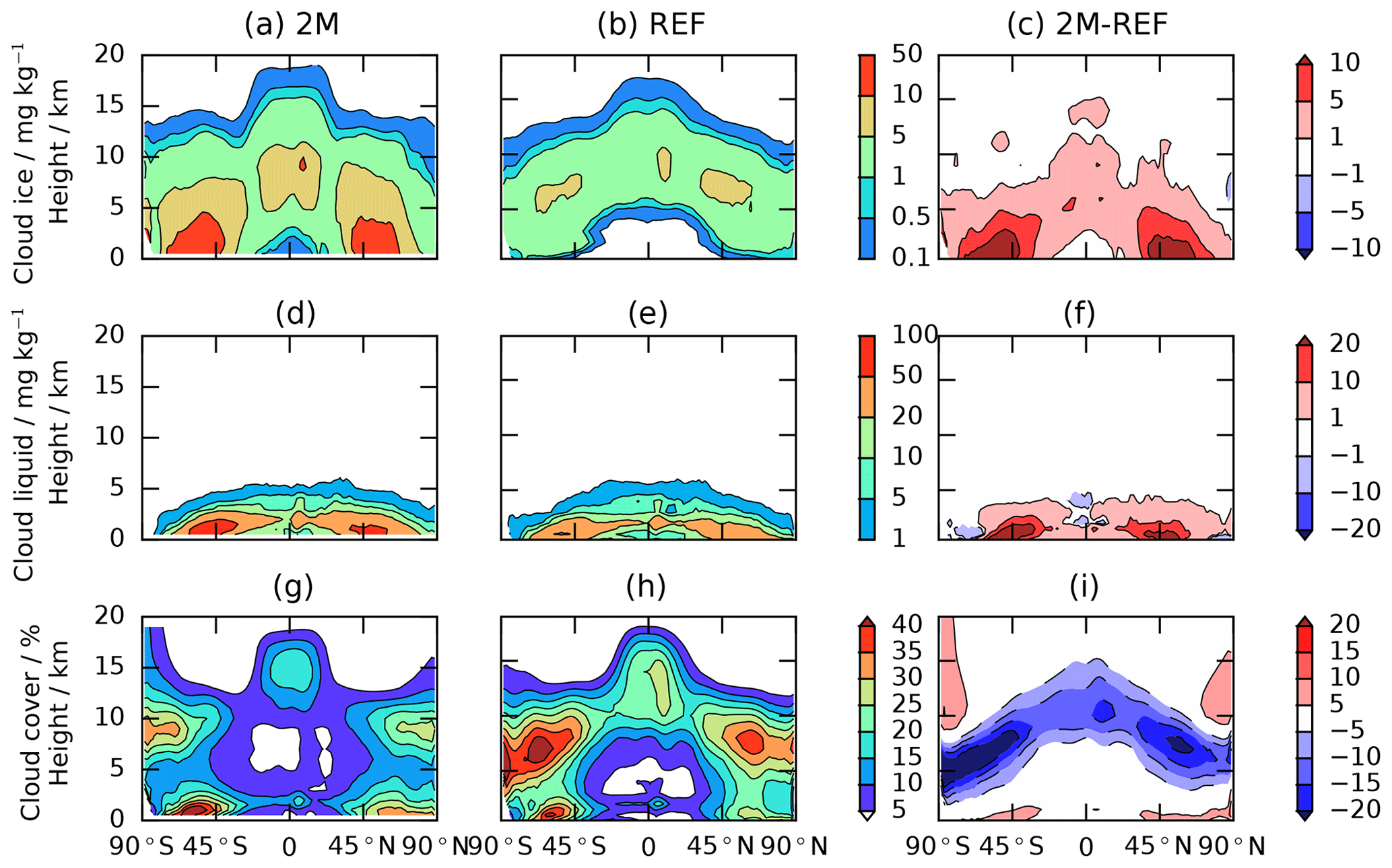
Figure 2The 10-year zonal mean cloud ice water content (a, b, c), cloud liquid water content (d, e, f) and cloud cover (g, h, i) for the new model (2M configuration; a, d, g), the reference model (REF; b, e, h) and differences between the two schemes (c, f, i).
In the simulated cloud liquid water there is no structural difference; the 2M simulation has substantially higher values everywhere. As the warm phase is not directly affected by the changes in cloud ice and the cloud cover parametrization, the differences are due to different autoconversion tuning parameters (γr in Table 2) and interactions with the new cloud cover and ice phase parametrizations.
The cloud cover differs significantly due to the new cloud cover parametrization in the new model. Differences are most pronounced in the cirrus regime where a cloud now only covers the entire grid box at the high supersaturation needed for homogeneous nucleation of solution droplets (see Sect. 2). Since this leads to a substantial difference in the cirrus cloud cover, we compare the reference model and the 2M configuration of the new model to satellite data in the following. For this purpose, we make use of the Cloud Feedback Model Intercomparison Project (CFMIP) Observation Simulator Package (COSP) (Bodas-Salcedo et al., 2011), which has already been implemented in ECHAM6-HAM2, and compare its output to the appropriate satellite product; the Cloud–Aerosol Lidar and Infrared Pathfinder Satellite Observation (CALIPSO), i.e. the GCM-oriented CALIPSO cloud product (GOCCP) (Cesana and Chepfer, 2013). Using a simulator allows for a consistent comparison of model output and satellite-derived cloud fields by minimizing artificial biases introduced by different cloud diagnostics and accounts for instrument sensitivity, which is particularly important for CALIPSO to account for the attenuation of the lidar signal.
The comparison to the cloud cover climatology from 2008 to 2014 of the CALIPSO-GOCCP product in Fig. 3 reveals that the new scheme fits better to the observed cloud structure (higher Pearson correlation coefficient ρ=0.75 and lower root mean squared error RMSE=4.0 % in the new model as compared to ρ=0.72 and RMSE=6.4 % in the reference model), despite an overall underestimation of cloudiness. It is worth noting that this underestimation is a consequence of the new cloud cover parametrization and not a result of model tuning. The distinct transition from the negative to positive bias between 5 and 10 km in the cloud fraction of the reference simulation is a consequence of the discontinuous description of cloud cover from the mixed-phase temperature regime (0 to −35 ∘C) to the cirrus regime (colder than −35 ∘C) that has been removed by the new scheme. Despite this improvement in terms of the vertical cloud structure, we find that the total cloud cover is worse in the new model. Figure 4c shows that the total cloud cover differs less between the two models than their difference in high cloud cover. This is probably due to the vertical overlap of high-level clouds with mid- and low-level clouds that already cover the entire grid box. In areas where there are no mid- and low-level clouds, the large amount of high-level clouds in the reference model can partly offset the overall underestimation of the total cloud cover. As a result, the reference model performs better in terms of RMSE for this variable. This is in agreement with Cesana and Waliser (2016), who find that climate models produce too few cloudy columns but that the clouds cover more vertical levels when present.
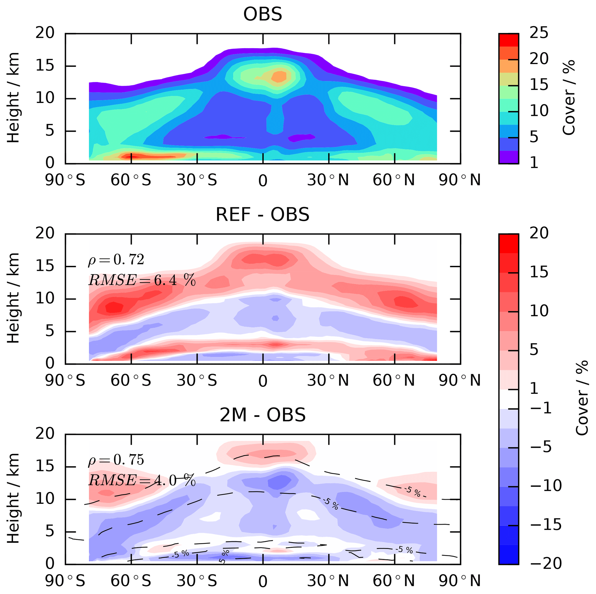
Figure 3Comparison of the simulated cloud fraction for simulations with the 2M configuration of the new model and the reference model (REF) for 10 years (2003–2012) and the CALIPSO-GOCCP satellite product (day and night, 7 years, 2008–2014). Model output is computed using the COSP simulator. The Pearson correlation coefficient (ρ) and root mean square error (RMSE) of the full, three-dimensional cloud cover climatology are computed for both models and shown in the difference plots. The dashed line indicates the area where there is a large (more than 5 %) difference between the 2M and REF simulations as shown in Fig. 2i.
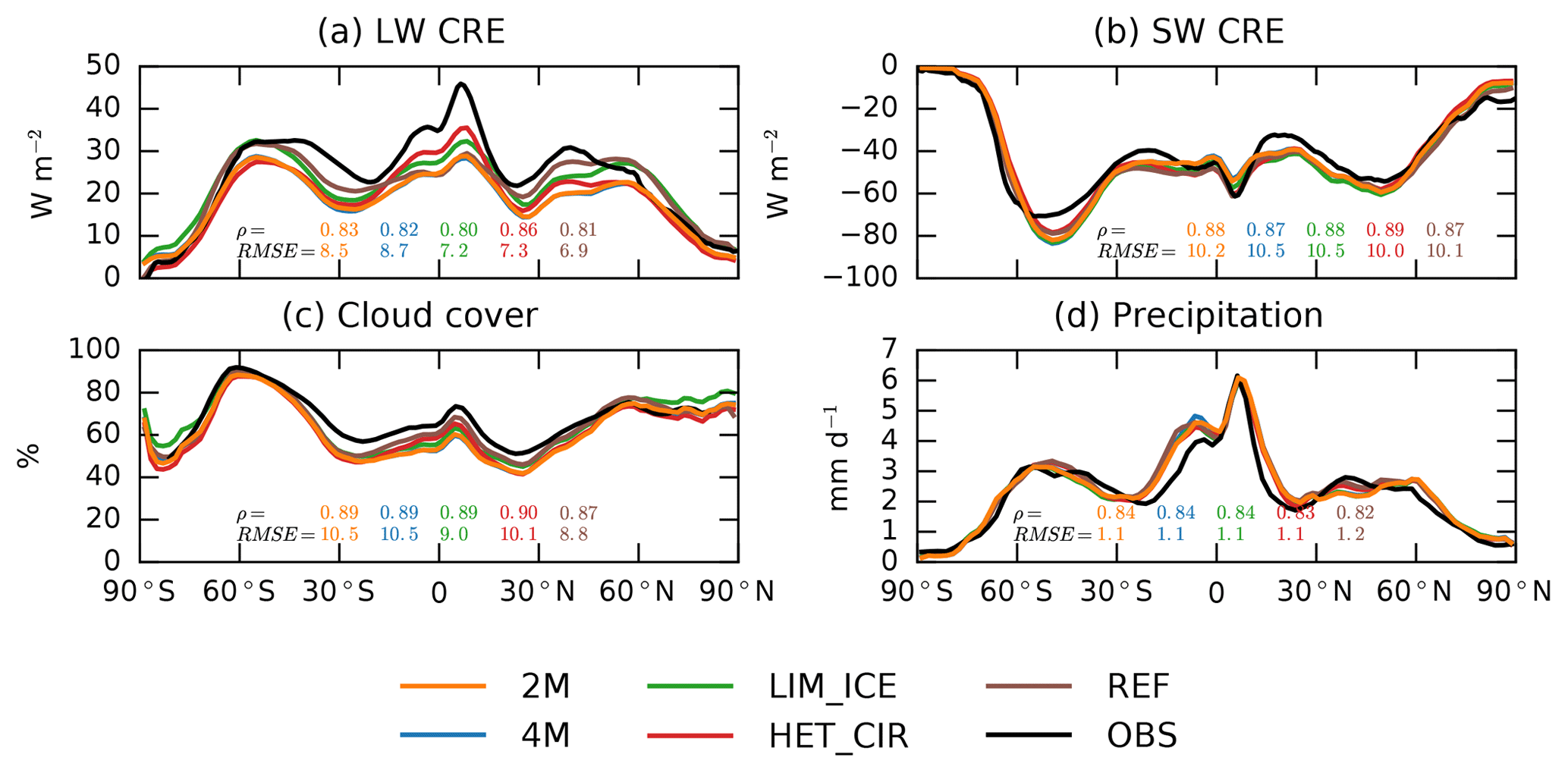
Figure 4The 10-year zonal mean values for longwave (LW CRE) and shortwave cloud radiative effects (SW CRE) (a, b) and total cloud cover and precipitation (c, d). The coloured lines show simulations of different configurations of the new model in Table 2. Black lines show satellite products. For CRE we show data from CERES EBAF (2000 to 2017). Total cloud cover is shown for CALIPSO-GOCCP (2006 to 2012) and the model data are produced using the COSP-simulator. Precipitation data are from the GPCP (2003 to 2012). The Pearson correlation coefficient and root mean square error are reported by text in matching colours for the different simulations and computed using the full two-dimensional fields.
3.3 Model tuning strategy
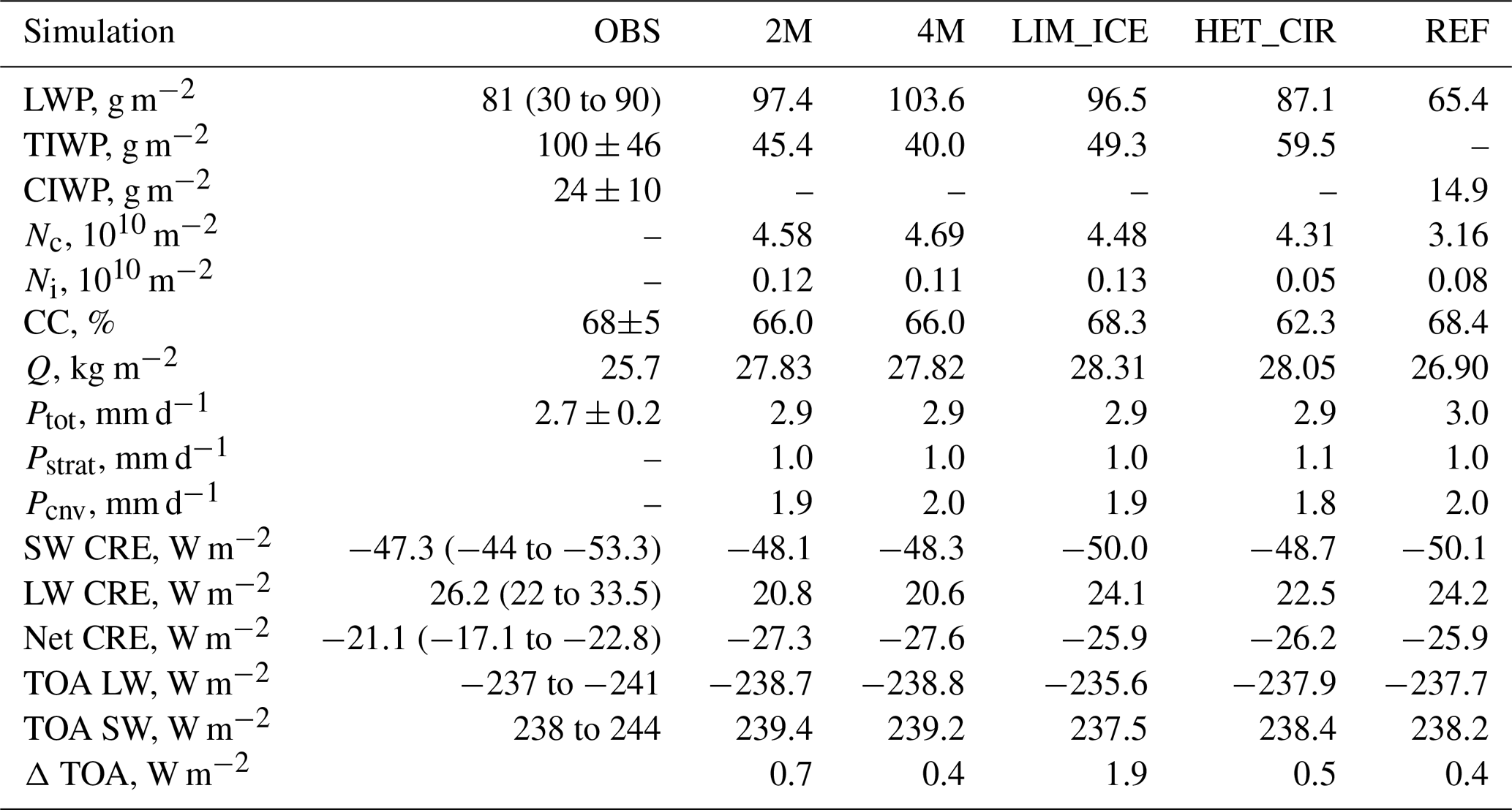
Model tuning has been conducted for the reference model (REF) and the two configurations of the new model, 2M and HET_CIR, while the 4M and LIM_ICE configurations use the same tuning as 2M. A summary of global, annual mean quantities is shown in Table 3. The main target of the tuning process has been the global, annual mean shortwave (SW) and longwave (LW) fluxes at TOA as well as the sum of the two. With the tuning parameters summarized in Table 2 we have a direct handle on the global, annual mean cloud radiative effect (CRE) at TOA, defined as the difference of all-sky and clear-sky radiative fluxes. To reach our SW and LW radiation as well as the radiation imbalance tuning targets at TOA, we adjust the CRE. A consequence of this tuning strategy is that all model simulations (including the reference model with a substantially different microphysics scheme) have a net CRE roughly between −26 and −27 W m−2 (depending on the achieved imbalance), which is more negative than any of the observational estimates and points at a structural problem in the model which is not specific to the microphysics scheme.
Table 3The 10-year global average values for a selection of key microphysical parameters for the model configurations presented in Table 2. Observational data are used from the compilation of Lohmann and Neubauer (2018) with the exception of ice water contents where we use the dataset of Li et al. (2012) and report their average standard deviation.
We compare the simulated zonal, annual mean precipitation to the Global Precipitation Climatology Product (GPCP) (Adler et al., 2018) for the years 2003 to 2012. Total precipitation is largely governed by the rate of evaporation at the surface. As the sea surface temperature is prescribed and most evaporation occurs over the oceans, cloud microphysics and convection parametrizations must produce similar amounts of total surface precipitation.
The lower cloud cover of the 2M and 4M simulations as compared to the LIM_ICE simulation is a direct consequence of the coupling of cloud ice and cloud cover. There are two main contributors: (1) the LIM_ICE configuration does not link the sedimentation sink of cloud ice to cloud cover while the other configurations (2M, 4M and HET_CIR) do and (2) the LIM_ICE configuration limits depositional growth of ice crystals and therefore the removal of water vapour by ice sedimentation is weaker, leaving more humidity in the atmosphere which in turn leads to more clouds.
For the TOA energy fluxes we use the climatology from 2000 to 2017 from the Clouds and the Earth's Radiant Energy System (CERES) Edition 4.0 Energy Balanced And Filled (EBAF) (Loeb et al., 2018) product for the model evaluation.
Without the overestimation of cirrus cloud cover, we can reduce the convective rain formation rate γcpr to values closer to the pure ECHAM6 (without online aerosols from the HAM model and a single-moment cloud microphysics scheme; see Stevens et al., 2013) model with a value of s−1 (Mauritsen et al., 2012). This allows more water vapour to be retained in the updraught cores, thus enhancing the formation of tropical cirrus clouds in the outflow regions of convective anvils, associated with a more pronounced peak in the LW CRE in the tropics (Fig. 4). However, the correlation coefficients with the CERES EBAF dataset are very similar to the reference model while the RMSEs are larger in all configurations of the new model. This is most likely a consequence of the different tuning in the two models. In the reference model both LW and SW CRE are stronger while the TOA fluxes are at the lower end of the tuning target in terms of magnitude; see Table 3.
3.4 Cloud ice
In Fig. 5 we evaluate the representation of cloud ice in the new model against the dataset compiled from CloudSat and CALIPSO retrievals by Li et al. (2012). This dataset is based on three different cloud water content products: 2B-CWC-RO4 (Austin et al., 2009), DARDAR (raDAR/liDAR) (Hogan, 2006; Delanoë and Hogan, 2008, 2010) and 2C-ICE (Deng et al., 2013). This dataset has the advantage that considerable effort has been put into the distinction between in-cloud ice in stratiform clouds (CIWC) and snow from stratiform clouds and convective cores (TIWC). The latter can usually not be diagnosed in models which treat snow formation diagnostically. The new single-category ice scheme used in this study only predicts the total stratiform ice water content, including snow. Therefore TIWC is most meaningful for a comparison with this model in the extra-tropics, where the contribution from convective snow is rather small. The reference model predicts stratiform cloud ice explicitly but diagnoses the snow mass flux. Therefore we can make full use of the distinction by Li et al. (2012) and compare the reference model to CIWC.
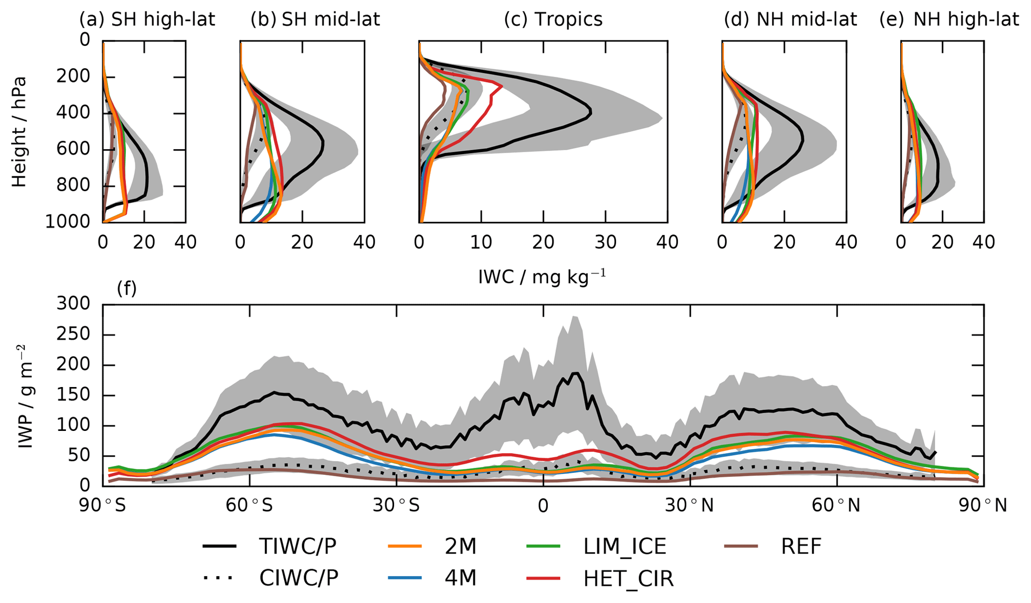
Figure 5Ice water content and ice water path compiled from observations by Li et al. (2012) and different versions of ECHAM6-HAM2 (10-year zonal averages) with the new microphysics scheme and the reference model. Panels (a)–(e) show vertical profiles for ice water content, panel (f) shows ice water path. The observations in black include total ice water content/path (TIWC/P; solid lines) and cloud ice water content/path (CIWC/P; dotted lines). Colours show total (stratiform) ice water content from the new model and cloud ice water content from the reference model. The grey shaded areas represent the average standard deviation as reported by Li et al. (2012). The profiles are averaged over different latitude bands: SH high-lat (80 to 60∘ S), SH mid-lat (60 to 30∘ S), tropics (30∘ S to 30∘ N), NH mid-lat (30 to 60∘ N) and NH high-lat (60 to 80∘ N).
Comparing the different simulations of the new scheme, we see that the 2M and 4M simulations are very similar both in terms of ice water content profiles (Fig. 5a–e) and ice water path (TIWP and CIWP respectively; Fig. 5f). The effect of riming on the ice crystal properties is most evident in the mid-latitudes. There, the 4M configuration produces rimed or partially rimed particles with higher fall speeds, which results in a reduced ice water content in the lower atmosphere (below roughly 700 hPa), as compared to the 2M configuration, where riming does not affect particle properties and thus fall speeds. However, the overall similarities suggest that the increased computational cost of the 4M configuration (see Table 2) and parametrization complexity (four versus two prognostic ice moments) do not significantly improve the overall representation of cloud ice in the GCM.
As explained in Sect. 2, the new cloud cover parametrization couples the cloud fraction to the ice water content. The aggregation parametrization depends on the concentration of ice crystals , which in turn is computed from the grid box mean value as , i.e. . We denote the parametrized source and sink terms by i.e. the partial time derivative ∂t of cloud ice qi restricted to one process. This leads to an artificial feedback loop: aggregation reduces Ni and increases ice particle size and fall speed and thus the sedimentation sink. Because cloud ice is linked to cloud cover (see the definition of s1 in Table 1, which replaces sw in Eq. (1) in the new cloud cover parametrization) the sedimentation of cloud ice decreases the cloud fraction b which in turn increases the in-cloud Ni and the ice crystal aggregation rate Sagg artificially. This feedback is the main contributor to the overall slightly lower ice water contents in 2M simulation as compared to the LIM_ICE simulation, which does not have this feedback, and outweighs the effect from the additional humidity that is available for ice growth in the 2M simulation. We acknowledge the existence of this artificial increase in the in-cloud Ni by sedimentation and the resulting feedback, but do not consider it to be important enough to sacrifice the physical correctness of the method used in the 2M configuration.
The most prominent differences between our simulations and the observations are in the tropics. As can be seen from Table 3, two-thirds of the entire surface precipitation is produced by the convective scheme. Since convective precipitation is a diagnostic quantity which is not included in the total ice water content here, a direct comparison of modelled, stratiform IWC/IWP with the observations is limited. With that in mind, we find that the 2M and 4M configurations of the new model underestimate the observed TIWP by roughly a factor of 3 in the tropics (Fig. 5). This is true for both the new model and the reference model (which has to be compared to CIWP/CIWC). Higher values for TIWP are produced by the LIM_ICE and HET_CIR simulations. While the slightly higher values in the LIM_ICE simulation are due to the cloud-fraction–sedimentation feedback explained above, the IWC values in the HET_CIR simulations are almost twice as large as in the 2M or 4M configurations and are a result of the lower ice supersaturation needed for ice crystals to nucleate heterogeneously. This allows for a more frequent formation of ice clouds at cold temperatures.
In the extra-tropics, the stratiform IWC is more representative of the observed TIWC/TIWP and we find slightly better agreement between the models and observations (Fig. 5). The vertical profile of TIWC in the mid-latitudes and high latitudes is not reproduced by the new model in any configuration, a feature shared with many CMIP5 models (Li et al., 2012), while the reference model performs rather well and only slightly underestimates the ice water path in mid-latitudes.
On the basis of the evaluation above, we choose the 2M configuration as default for the new model for its computational efficiency compared to the 4M configuration and physical correctness compared to the LIM_ICE configuration. Heterogeneous nucleation of ice crystals at low ice supersaturation in the cirrus regime (parametrized in the HET_CIR configuration) can be included optionally for future work with the new model and yields promising results but is not used for the analysis in Sects. 4 and 5 since it is in part based on unpublished work.
3.5 Cloud liquid water
We compare the simulations with the new and the reference model to the Multisensor Advanced Climatology of Liquid Water Path (MAC-LWP) (O'Dell et al., 2008; Elsaesser et al., 2017); see Fig. 6. Microwave sensors cannot reliably distinguish precipitation from cloud water. Therefore we only evaluate regions with low precipitation, i.e. where the liquid water path (LWP) and total water path (TWP) have similar magnitude. We use the threshold suggested by Elsaesser et al. (2017). The differences in liquid water are very small for the different configurations of the new model, so we only evaluate the default configuration 2M. We find an overall high bias in LWP in the extra-tropics for both models but a more pronounced effect in the new model. As discussed above, the TOA energy balance constraints in the new model require a lower tuning parameter for the autoconversion of cloud droplets to rain (γr) and thus thicker liquid clouds that reflect more SW radiation. We consider this the main reason for the higher liquid water path in the 2M as compared to the REF simulation, as the warm phase parametrizations are the same in both models.
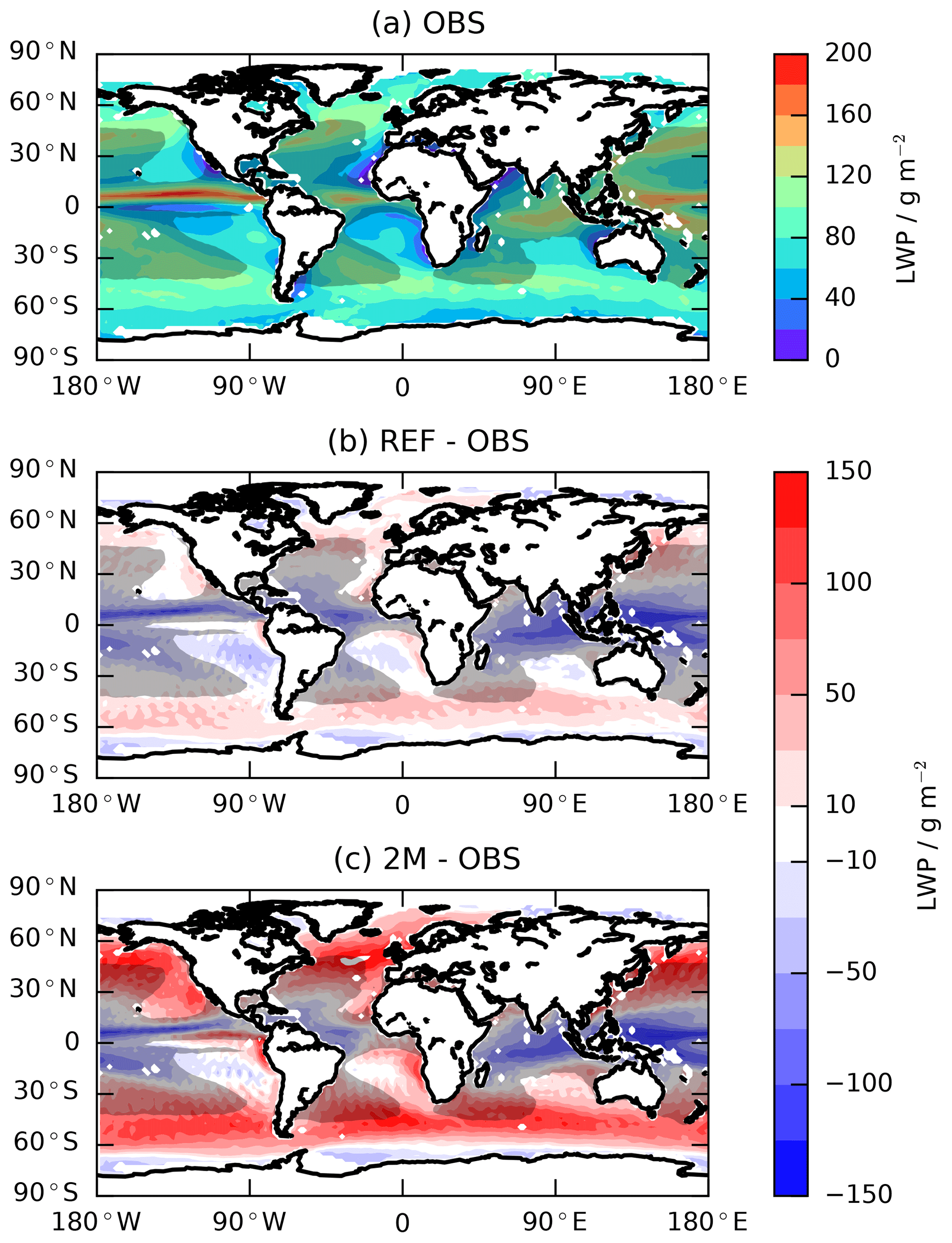
Figure 6LWP as observed by the Multisensor Advanced Climatology of LWP (MAC-LWP), climatology from 2003 to 2012. Panel (a) shows the observations, (b) shows the difference between the new model (2M) and the observations, and (c) shows the difference between the reference model and the observations. The models are both run for 10 years from 2003 to 2012. The grey shaded areas show regions where the liquid water path is dominated by precipitation (), i.e. where there is no reliable estimate for in-cloud liquid water path.
In the Southern Ocean, the overestimation of LWP translates into an overestimation of the SW CRE, evident from Fig. 4b. Note that the REF simulation with a smaller positive LWP bias overestimates SW CRE less.
3.6 Cloud phase partitioning
Different climate models produce a wide range of ice-to-total-cloud fractions (McCoy et al., 2016). Here we examine the histograms of the ratio of cloud phase (PR; relative fraction of ice clouds to total clouds) to temperature (T) used in the model intercomparison by Cesana et al. (2015) (their Fig. 10) in Fig. 7, where the wide variety of different cloud distributions in PR–T histograms among models has been highlighted. In this section we discuss the distributions produced by our models and compare the simulated average cloud phase ratio per temperature to the CALIPSO-GOCCP satellite product.
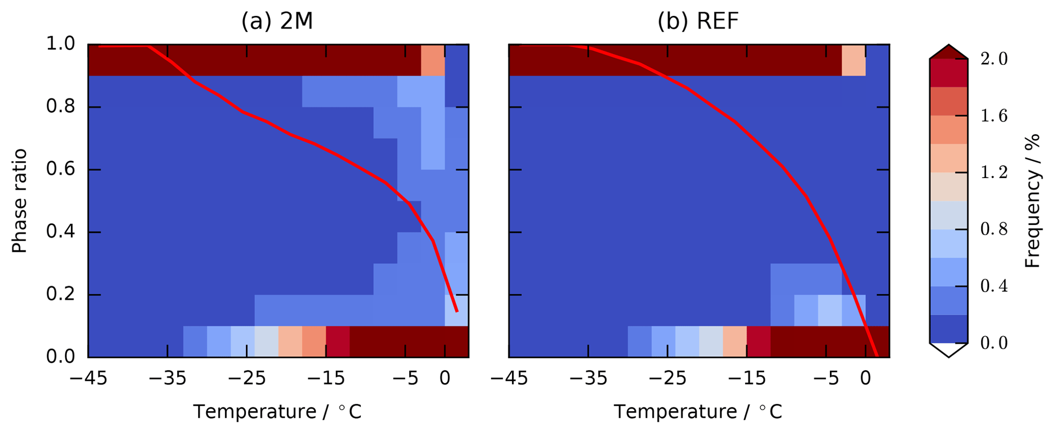
Figure 7Frequency of cloud occurrence per temperature and phase ratio for histogram bin widths of 3 ∘C and 0.1, respectively. The average ice fraction per temperature bin is shown by the red line for the new model (2M; a) and the reference model (REF; b). The data have been accumulated over 10 years of simulation from 2003 to 2012.
The different configurations of the new model have very similar PR–T histograms, which is why we only show the one for 2M. For the new model we only count cloudy regions, i.e. require b>0, to exclude falling ice (snow) with PR=1. Comparing the 2M to the REF simulation in Fig. 7 shows that the 2M simulation produces slightly less supercooled liquid cloud at warm temperatures above −15 ∘C but slightly more at temperatures below −15 ∘C. In contrast to REF, where any ice above 0 ∘C melts instantly, the finite melting rate employed by the 2M configuration allows for cloud ice at temperatures warmer than 0 ∘C.
Most clouds are either liquid or fully glaciated; mixed-phase states are rare in our models as well as the satellite product, assuming that the undefined-phase clouds are considered as mixed-phase clouds (Cesana et al., 2016). Due to the finite melting rate employed in the new model not all ice crystals melt entirely within one model time step, making mixed-phase states at these warm temperatures around 0 ∘C slightly more frequent as compared to the reference model. Nevertheless, the full PR–T histogram does not contain significantly more information than the average phase ratio per temperature.
In Fig. 8 we compare the simulated cloud phase partitioning to the lidar observations from the CALIPSO satellite (CALIPSO-GOCCP product). To allow for a quantitative comparison, we used the COSP lidar simulator, which minimizes the differences between model output and the satellite product due to different sampling methods and lidar attenuation. As suggested by Cesana et al. (2016) we counted the clouds in the undefined cloud phase category in the satellite product as well as the COSP output as completely glaciated. The cloud phase ratio obtained from the lidar simulator in this manner is consistently smaller than the observations. In the following sections we will provide tools to identify which parametrized processes are most likely controlling the structure of this distribution.
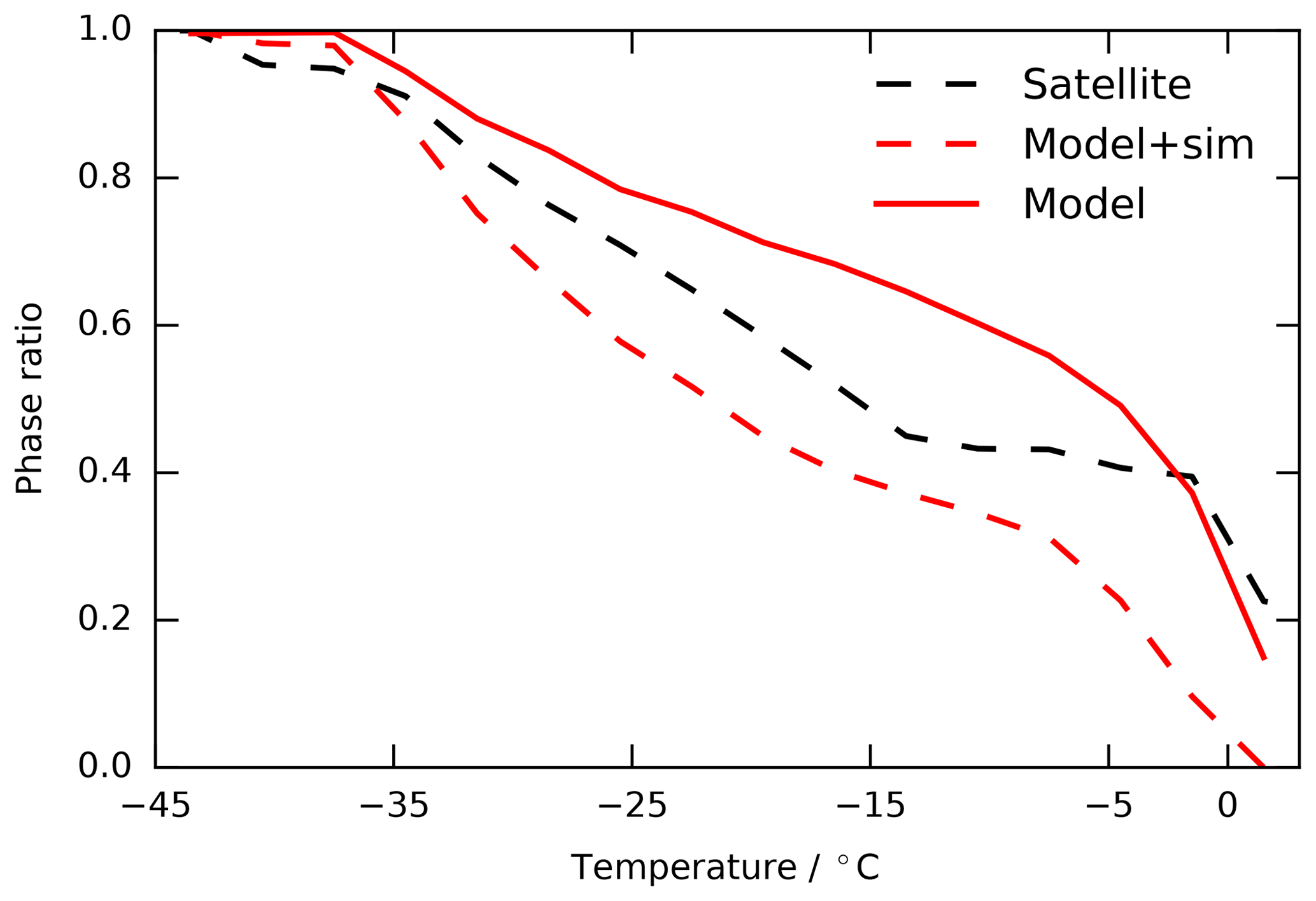
Figure 8Cloud phase ratio per temperature for histogram bin widths of 3 ∘C. The average ice fraction per temperature bin is shown for the model data (red, solid line), the CALIPSO-GOCCP product (black, solid line) and the output from the COSP simulator applied to the model (red, dashed line). For both the model and satellite data we assumed that clouds with undefined phase as classified by the lidar simulator or retrieval algorithm are dominated by ice and thus contribute to the ice phase (Cesana et al., 2016)
The microphysical properties of a cloud are defined by the cloud formation processes, i.e. the cloud is simply the product of its formation history. Traditionally, model output reveals a snapshot of the simulated cloud field at any given time. Due to the finite storage capacity, aggregates of the model states are stored and information on the integration from process rates is lost. Most common are temporal averages (e.g. monthly or yearly mean values) or vertical aggregates (e.g. burden, total cloud cover, TOA, and surface radiative fluxes or precipitation). The aggregated cloud states are then compared to observations to infer information about the microphysical parameterizations leading to the cloud state. Inferring the dominant processes responsible for a model-to-observation mismatch is difficult. Usually it is very time consuming because many sensitivity studies are necessary where processes are turned off individually and even then the interaction and competition between processes cannot be assessed. Ultimately, spatio-temporally averaged model output defeats the purpose of simulating any physical system: finding cause and effect between differential equations and observables.
In this section we tackle the problem the other way around. Instead of inferring the formation history based on the current cloud state, we make use of additional prognostic equations to store and quantify ice formation pathways. This information can then be used to compute conditional probabilities to provide a sound cause-and-effect relation between the microphysical parameterizations and the resulting cloud state. This analysis makes direct inference from observables on cloud microphysical parameterizations tangible.
Our model parameterizes three fundamentally different source terms for cloud ice: heterogeneous contact and immersion freezing of cloud droplets in the mixed-phase regime Shet−frz, homogeneous freezing of cloud droplets Shom−frz, and nucleation of ice from deliquesced aerosols Snuc. The latter two processes are restricted to temperatures below −35 ∘C while heterogeneous freezing dominates at warmer temperatures. Note that we focus on the mixed-phase regime and thus do not further separate heterogeneous from homogeneous ice nucleation in the cirrus regime, even though nucleation of cloud ice on mineral dust is implemented in the HET_CIR configuration.
To distinguish ice that formed by either of the process rates above, we introduce two additional prognostic tracers to keep track of the formation history of the cloud mass at any given time in the simulation.
4.1 Mixed-phase heterogeneous freezing origin mass fraction
To separate cloud ice that formed in the mixed-phase temperature regime we introduce the heterogeneously nucleated ice mass mixing ratio qi,het governed by the following equation:
The growth of this tracer depends on the ice mass source and sink terms for collisions with cloud droplets Scol, vapour deposition Sdep, sublimation Ssub and the fraction of cloud ice that has already formed previously by heterogeneous freezing, defined as . We abbreviate the partial derivative with respect to the vertical dimension z (in m) by ∂z. The tracer sediments along with the total ice mass with the mass-weighted terminal velocity vm in metres per second (m s−1). Convectively detrained ice is missing here due to a lack of an explicit, aerosol-dependent freezing parameterization in the convection scheme. Water is only detrained as ice below temperatures of −35 ∘C where we assume that liquid water freezes homogeneously.
4.2 Liquid origin mass fraction
We further distinguish between cloud ice that forms via homogeneous freezing of cloud droplets and ice that nucleates in situ from deliquesced aerosol. This allows in situ cirrus to be disentangled from liquid origin cirrus. To quantify the ice mass fraction initiated through freezing of liquid water, we implement a tracer governed by the following equation:
We sum up all liquid to ice mass source terms, namely homogeneous freezing of cloud droplets Shom−frz and convective detrainment of cloud ice Sice−cv together with the processes defined above. The liquid origin mass fraction is given by .
4.3 Cloud types based on the cloud formation history
The additional information on the cloud formation history from Eqs. (5) and (6) can be combined with the liquid fraction , cloud vertical thickness (i.e. the pressure difference between cloud base pbase and cloud top ptop) and cloud top temperature Ttop to build an inclusive set of cloud types. As is evident from Fig. 7, mixed-phase clouds are unstable due to the WBF process, leading to a strongly bimodal distribution of the frequency of phase ratio occurrence. This bimodality exists but is less pronounced for the ice mass source fractions Fhet and Fliq−o shown in Fig. 9 together with the liquid fraction Fliq. Ice source mass fractions between zero and one arise from competing formation mechanisms and mixing of clouds of distinct sources.
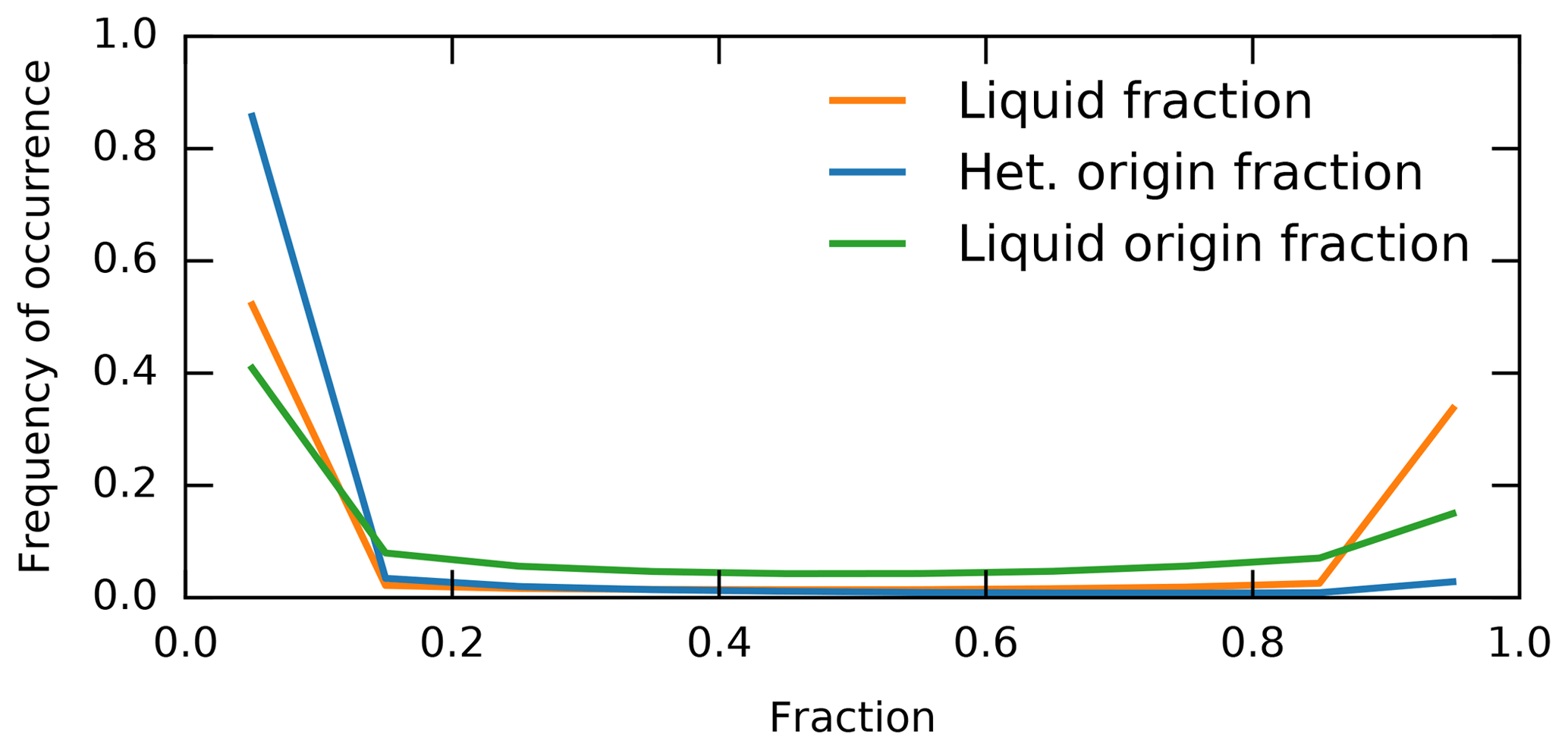
Figure 9Frequency of cloud occurrence per ice source fraction for the liquid origin fraction Fliq and the different ice source fractions Fhet and Fliq−o. The histogram bin width is 0.1. The lines are aligned with bin centres. Only grid boxes are sampled where all the fractions are well-defined, i.e. only cloudy grid boxes for Fliq and only grid boxes containing ice for Fhet and Fliq−o. Data are sampled every time step for 10 years of simulation with the new model (2M).
We make use of the separation of cloud occurrence frequency in the five-dimensional parameter space (Fliq, Δp, Fhet, Fliq−o, Ttop) to classify clouds into the types defined in Table 4. The labels are based on the analysis of the temperature regime each cloud primarily occurs in and are discussed in more detail below.
Table 4Definition of cloud types. We categorize and separate clouds by exceeding thresholds of the five predictors: the heterogeneous freezing origin fraction Fhet, cloud top to bottom pressure difference Δp, cloud liquid fraction Fliq, liquid origin fraction Fliq−o and the cloud top temperature Ttop. If a predictor is not used for a certain class, it is symbolized by a “–” sign.

The classification is computed online and thus allows statistics to be accumulated per cloud type. Examples of such statistics are the cloud top temperature, liquid fraction and liquid origin fraction distributions per cloud type shown in Fig. 10. These distributions allow physical properties of each cloud type and its associated formation pathway to be identified. Below we use them to justify the cloud type labels in Table 4.
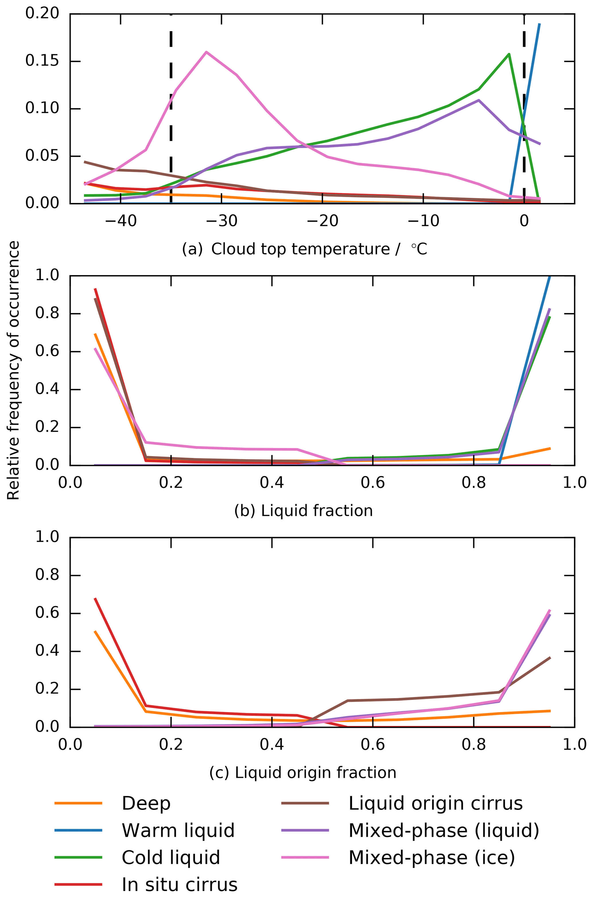
Figure 10Relative frequency of cloud occurrence (normalized by the cloud type occurrence frequency). This corresponds to conditional probability histograms, for the model state X with components X•: cloud top temperature (a), liquid fraction (b) and liquid origin fraction (c) for each cloud type i. Bin widths are 3 ∘C for temperature and 0.1 for the dimensionless fractions respectively; lines are aligned with bin centres. Data are sampled every time step for 10 years of simulation with the new model (2M).
Homogeneously nucleated clouds are separated into three classes. They are labelled cirrus if they are thinner than 500 hPa, otherwise we refer to them as deep. This name arises from the fact that the vast majority of such clouds have cloud tops that are colder than −35 ∘C as can be seen in Fig. 10a. We further differentiate between in situ cirrus, clouds that nucleated from deliquesced aerosols or formed heterogeneously below −35 ∘C in the case of the HET_CIR simulation (not shown), and liquid origin cirrus, clouds that formed from homogeneous freezing of cloud droplets. While there is a clear peak for clouds that formed without any liquid water precursors (), the peak for complete liquid origin clouds is less pronounced due to competing primary ice source terms (Fig. 10c).
Heterogeneously nucleated clouds are separated into two classes. We find two distinctly different cloud types where ice formed predominantly from heterogeneous freezing of cloud droplets. As shown in Figs. 7 and 9, a truly mixed state with liquid water and ice is unstable and thus rare. Therefore we divide heterogeneously nucleated clouds into those that are dominated by liquid water and ice respectively; see Fig. 10b. We label them both as mixed-phase (liquid and ice dominated respectively) since the cloud tops of such clouds are predominantly found in the mixed-phase temperature regime between 0 and −35 ∘C. Liquid clouds are further separated into those with cold cloud tops (T<0 ∘C) and warm cloud tops (T>0 ∘C).
In the following sections we will use the cloud types and associated formation pathways described here to gain insights into the simulated cloud fields. It is crucial to keep in mind that the labels provided for the cloud types here are based on formation pathways. This is in strong contrast to the traditional definitions based exclusively on the cloud state and can thus lead to results that seem counterintuitive at first. For example, cirrus clouds are commonly defined as clouds with temperatures colder than −35 ∘C (or more generally the temperature below which homogeneous freezing becomes efficient, depending on the model). Here we only require cirrus clouds to form by the processes that are typically found at temperatures below −35 ∘C and subsequently track their evolution without imposing strict temperature constraints. This means, however, that a cirrus cloud is still called cirrus, even if its constituent ice crystals fall far into the mixed-phase regime.
We implemented the additional prognostic tracers needed to quantify ice formation pathways introduced in the last section in the new model. Along with the new microphysics scheme we introduced a new code structure which removed the sequential computation of microphysical tendencies in the reference model and clearly segregates the computation of microphysical tendencies and local model state updates (Dietlicher et al., 2018). This allows additional tracers to be easily implemented. Although we did not implement the same tracers in the reference model as well, we expect that the insights gained from this section can be transferred to the reference model since many aspects of the model are the same or very similar, e.g. the diffusion, convection and cloud cover parametrizations (except in the cirrus regime).
With the additional prognostic equations to identify ice formation pathways and the cloud types derived thereof, we are able find the microphysical causes for the macrophysical cloud states simulated by the new model. A clear causal relationship between the simulated cloud fields and the underlying parametrizations is critical for model development. Improving the representation of sub-grid processes is usually a two-step process: first, observational data are used to evaluate the simulated cloud fields and then model sensitivities are assessed to find the parametrizations responsible for potential model-to-observation mismatches. In the following we demonstrate how the ice formation pathways introduced in the last section can be used for the second step using the example of the phase ratio discussed in Sect. 3 and Fig. 7.
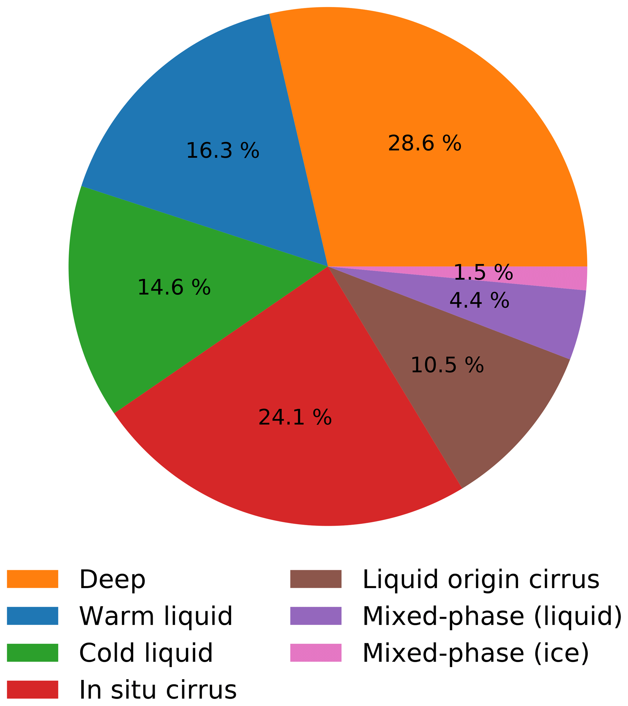
Figure 11Global relative contribution to the 3-D cloud volume (as measured by the air mass occupied) for the cloud types defined in Table 4 based on their formation pathways. Data are sampled every time step for 10 years of simulation with the new model (2M).

Figure 12Same as in Fig. 5 but for the absolute frequency of occurrence profile (a–e) and relative contribution to the total cloud cover (f). The relative contribution is computed as the fraction of cloud volume occupied per column and cloud type. Data are sampled every time step for 10 years of simulation with the new model (2M).
5.1 Relative cloud type frequencies
We classify the clouds online according to Table 4 to generate a global climatology of the relative contributions of each formation pathway to the 3-D cloud volume (defined as the air mass covered by the cloud) in Fig. 11. From this pie chart it is evident that the majority of the cloud population consists of homogeneously nucleated ice clouds (in situ cirrus and deep clouds) and liquid clouds. The next smallest class is the liquid origin cirrus clouds, making up 10.5 % of the cloud population or almost one-third of all cirrus clouds. Mixed-phase clouds only contribute roughly 6 %, with the fraction of such clouds that are dominated by ice being smaller than those being dominated by liquid water.
We also show zonal means of the cloud type occurrence frequencies in Fig. 12. This view sheds more light on where each formation pathway dominates. Liquid clouds with warm cloud tops dominate in the tropics while their cold top counterparts are primarily found in mid-latitudes. Due to abundant deep convection in the tropics, large amounts of liquid water are transported to high altitudes where homogeneous freezing of cloud droplets sets in, leading to a frequent occurrence of liquid origin cirrus clouds. Heterogeneous freezing only affects clouds at low altitudes where there is no competition with homogeneous nucleation. Seemingly inexistent are mixed-phase clouds where heterogeneous freezing of cloud droplets alone causes glaciation of the host liquid cloud.
5.2 Decomposing the cloud phase partitioning
By sampling the cloud types according to temperature we find the dominant parametrizations controlling the phase ratio in our model. Figure 13 decomposes the average liquid fraction per temperature bin (compare Fig. 8) into the different cloud types. Keep in mind that the cloud types are separated into mostly glaciated clouds (cirrus, mixed-phase (ice) and deep) and liquid clouds (warm and cold liquid as well as mixed-phase (liquid)) as shown in Fig. 10c. The most frequent cloud types simulated in the mixed-phase regime are deep clouds making up roughly 40 % of clouds throughout this temperature range. The second most frequent clouds are in situ cirrus, followed by liquid origin cirrus. The two heterogeneously nucleated mixed-phase cloud types make up the smallest fraction of clouds. The fact that we find homogeneously nucleated clouds with a vertical extent of less than 500 hPa (i.e. cirrus clouds) down to temperatures of 0 ∘C is in part due to the choice of the threshold value to separate cirrus clouds from deep clouds but does not affect the main conclusion: the dominant source term for cloud ice in the mixed-phase temperature regime is homogeneous freezing of deliquesced aerosols taking place at temperatures below −35 ∘C.
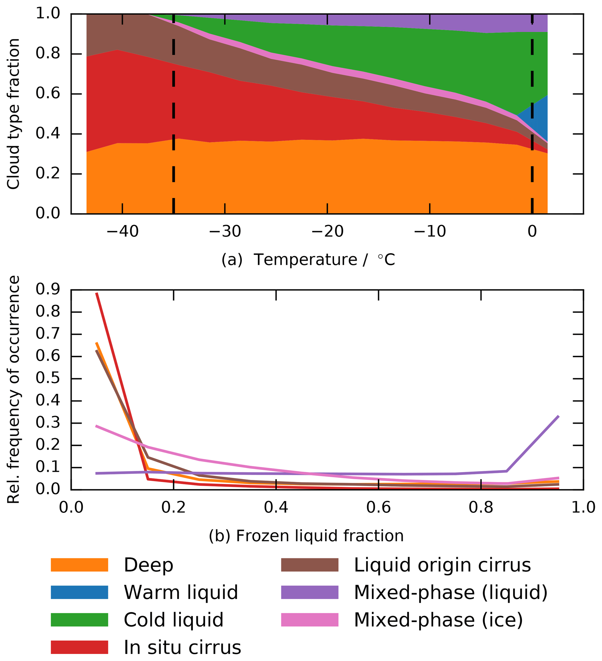
Figure 13Cloud type fraction as a function of grid box temperature (a) and frequency of occurrence of frozen liquid fraction (b). We only sample cloudy grid boxes, i.e. those with a cloud fraction component Xb>0. For the frozen liquid fraction component we show the relative frequency of occurrence . The latter is the accumulated ice mass fraction that formed through any liquid-water-to-ice conversion process (including the WBF process). Note that this is not equal to the liquid origin mass that quantifies the origin of cloud ice. Bin widths are 3 ∘C and 0.1 respectively; lines are aligned with bin centres. Data are sampled every time step for 10 years of simulation with the new model (2M).
Analogous to the prognostic tracers introduced in Sect. 4 and formally defined in Eq. (A1), we trace the state of water from which ice forms. The frozen liquid ice mass mixing ratio tracer accumulates the mass of liquid water that has been converted to ice by freezing, riming or the WBF process and allows the frozen liquid fraction to be computed as . For the majority of homogeneously nucleated clouds, the frozen liquid fraction is very small (<10 %), from which we conclude that ice predominantly forms directly from deposition of water vapour (excluding the WBF process) and thus without a liquid water precursor; see Fig. 13b. This implies that ice nucleated in the cirrus regime not only dominates glaciation in mixed-phase clouds but even inhibits the formation of supercooled liquid water clouds. As a result, contact and immersion freezing is limited to clouds with cloud tops warmer than −35 ∘C where there is no competition with sedimenting ice that formed in the cirrus regime.
Revisiting Fig. 8 we can come up with potential shortcomings of our model that could explain the underestimation of the ice fraction from the COSP simulator compared to observations. A straightforward explanation could be that our models simply underestimate the frequency of ice clouds. From what we learned from Fig. 13, the best candidate to increase the ice fraction at temperatures warmer than −25 ∘C are the cold liquid clouds. These clouds have cloud tops warmer than the temperature of homogeneous freezing, which makes immersion and contact freezing the only possible pathways to glaciation. This suggests that our model lacks INPs capable of nucleating ice in this temperature range. Another explanation could be that the cloud structure is unrealistic such that there is a substantial amount of cloud ice within the deep clouds which are optically thick due to their large vertical extent. In such clouds we expect the lidar signal to be completely attenuated which makes them partly invisible to the COSP simulator.
We presented the global performance of the new cloud microphysics scheme in the ECHAM6-HAM2 GCM introduced in D18. The main difference as compared to its predecessor is the consistent description of cloud ice using a single, prognostic category. Thus, it does not rely on poorly constrained conversion parametrizations between in-cloud ice and precipitating snow categories. Different from D18, we introduced a new approach to extend the sub-grid cloud cover scheme of Sundqvist et al. (1989) to ice clouds. This scheme no longer has the positive cloud cover bias at temperatures below −35 ∘C present in the reference model.
We assessed ice formation pathways quantitatively by introducing additional prognostic equations for the heterogeneously formed and liquid origin ice mass mixing ratios. We found that in our model the majority of cloud ice forms below −35 ∘C by either homogeneous freezing of cloud droplets or homogeneous nucleation of deliquesced aerosols. Only about 6 % of clouds form by contact and immersion freezing in mixed-phase temperatures, making homogeneous freezing the main source for cloud ice even at temperatures warmer than −35 ∘C. The Lagrangian perspective on the modelled cloud fields provided by the formation pathway analysis allowed in situ and liquid origin cirrus clouds to be distinguished. We found that roughly one-third of all cirrus clouds form by homogeneous freezing of cloud droplets.
Furthermore, ice formation pathways provide the causal link between the microphysical parametrizations and the resulting cloud fields. We showed how they can be used to break the simulated phase ratio down into the contributions of different microphysical parametrizations. We find that mixed-phase processes like the WBF process and heterogeneous freezing of supercooled cloud droplets play a minor role in our model because most ice originates in the cirrus regime. As a result, mixed-phase freezing parametrizations cannot control the average phase ratio per temperature. Their effect is superseded by the structure of ice clouds (with deep clouds making up most of the cloud ice in the mixed-phase regime) and the absence of INPs that could glaciate cold liquid clouds with cloud tops warmer than −35 ∘C.
The ECHAM6-HAMMOZ model is made available to the scientific community under the HAMMOZ Software Licence Agreement, which defines the conditions under which the model can be used. To obtain a license, please follow the instructions on https://redmine.hammoz.ethz.ch/projects/hammoz/wiki/1_Licencing_conditions (last access: 11 July 2019).
We not only diagnose the phase which initiated ice formation to separate liquid origin from vapour origin ice but also keep track of the total amount of liquid water that has been converted to ice with a separate tracer . The mass mixing ratio for frozen liquid water defined as follows:
Analogous to the tracers defined in Sect. 4, we define the frozen liquid fraction as . In contrast to the these tracers defined previously, the frozen liquid water mass mixing ratio contains information on ice growth history rather than source processes.
RD designed the experiments and developed the microphysics scheme and the cloud formation pathways analysis. DN and RD performed the model simulations. UL and DN provided scientific guidance. RD wrote the paper with comments from UL and DN.
The authors declare that they have no conflict of interest.
The ECHAM-HAMMOZ model is developed by a consortium composed of ETH Zurich, Max Planck Institut für Meteorologie, Forschungszentrum Jülich, University of Oxford, the Finnish Meteorological Institute and the Leibniz Institute for Tropospheric Research and managed by the Center for Climate Systems Modeling (C2SM) at ETH Zurich. Special thanks go to Sylvaine Ferrachat for technical support regarding the model. The computing time for this work was supported by a grant from the Swiss National Supercomputing Center (CSCS) under project ID s652 and from ETH Zurich. We thank Steffen Münch for providing his implementation of more advanced cirrus parameterizations for the sensitivity tests presented here. We obtained the CERES EBAF data from the NASA Langley Research Center CERES ordering tool at http://ceres.larc.nasa.gov/ (last access: 11 July 2019). The GPCP data have been provided by the NOAA-ESRL Physical Sciences Division, Boulder, Colorado, from their Web site at https://www.esrl.noaa.gov/psd/ (last access: 11 July 2019). Finally, we express our gratitude to the two anonymous reviewers for carefully reading our paper and valuable feedback which lead to a substantial improvement of the model evaluation.
This research has been supported by the Swiss National Science Foundation (grant no. 200021_160177).
This paper was edited by Toshihiko Takemura and reviewed by two anonymous referees.
Adler, R. F., Sapiano, M. R. P., Huffman, G. J., Wang, J.-J., Gu, G., Bolvin, D., Chiu, L., Schneider, U., Becker, A., Nelkin, E., Xie, P., Ferraro, R., and Shin, D.-B.: The Global Precipitation Climatology Project (GPCP) Monthly Analysis (New Version 2.3) and a Review of 2017 Global Precipitation, Atmosphere, 9, 138, https://doi.org/10.3390/atmos9040138, 2018. a
Ansmann, A., Tesche, M., Knippertz, P., Bierwirth, E., Althausen, D., Müller, D., and Schulz, O.: Vertical profiling of convective dust plumes in southern Morocco during SAMUM, Tellus B, 61, 340–353, https://doi.org/10.1111/j.1600-0889.2008.00384.x, 2009. a
Atkinson, J. D., Murray, B. J., Woodhouse, M. T., Whale, T. F., Baustian, K. J., Carslaw, K. S., Dobbie, S., O'Sullivan, D., and Malkin, T. L.: The importance of feldspar for ice nucleation by mineral dust in mixed-phase clouds, Nature, 498, 355–358, https://doi.org/10.1038/nature12278, 2013. a
Austin, R. T., Heymsfield, A. J., and Stephens, G. L.: Retrieval of ice cloud microphysical parameters using the CloudSat millimeter-wave radar and temperature, J. Geophys. Res.-Atmos., 114, D00A23, https://doi.org/10.1029/2008JD010049, 2009. a
Bodas-Salcedo, A.: Cloud Condensate and Radiative Feedbacks at Midlatitudes in an Aquaplanet, Geophys. Res. Lett., 45, 3635–3643, https://doi.org/10.1002/2018GL077217, 2018. a
Bodas-Salcedo, A., Webb, M. J., Bony, S., Chepfer, H., Dufresne, J.-L., Klein, S. A., Zhang, Y., Marchand, R., Haynes, J. M., Pincus, R., and John, V. O.: COSP: Satellite simulation software for model assessment, B. Am. Meteorol. Soc., 92, 1023–1043, https://doi.org/10.1175/2011BAMS2856.1, 2011. a
Boucher, O., Randall, D., Artaxo, P., Bretherton, C., Feingold, G., Forster, P., Kerminen, V.-M., Kondo, Y., Liao, H., Lohmann, U., Rasch, P., Satheesh, S., Sherwood, S., Stevens, B., and Zhang, X.: Clouds and Aerosols, book section 7, 571–658, Cambridge University Press, Cambridge, UK and New York, NY, USA, https://doi.org/10.1017/CBO9781107415324.016, 2013. a
Ceppi, P., Hartmann, D. L., and Webb, M. J.: Mechanisms of the Negative Shortwave Cloud Feedback in Middle to High Latitudes, J. Climate, 29, 139–157, https://doi.org/10.1175/JCLI-D-15-0327.1, 2016. a
Cesana, G. and Chepfer, H.: Evaluation of the cloud thermodynamic phase in a climate model using CALIPSO-GOCCP, J. Geophys. Res.-Atmos., 118, 7922–7937, https://doi.org/10.1002/jgrd.50376, 2013. a
Cesana, G. and Waliser, D. E.: Characterizing and understanding systematic biases in the vertical structure of clouds in CMIP5/CFMIP2 models, Geophys. Res. Lett., 43, 10538–10546, https://doi.org/10.1002/2016GL070515, 2016. a
Cesana, G., Waliser, D. E., Jiang, X., and Li, J.-L. F.: Multimodel evaluation of cloud phase transition using satellite and reanalysis data, J. Geophys. Res.-Atmos., 120, 7871–7892, https://doi.org/10.1002/2014JD022932, 2015. a, b, c
Cesana, G., Chepfer, H., Winker, D., Getzewich, B., Cai, X., Jourdan, O., Mioche, G., Okamoto, H., Hagihara, Y., Noel, V., and Reverdy, M.: Using in situ airborne measurements to evaluate three cloud phase products derived from CALIPSO, J. Geophys. Res.-Atmos., 121, 5788–5808, https://doi.org/10.1002/2015JD024334, 2016. a, b, c
Delanoë, J. and Hogan, R. J.: A variational scheme for retrieving ice cloud properties from combined radar, lidar, and infrared radiometer, J. Geophys. Res.-Atmos., 113, D07204, https://doi.org/10.1029/2007JD009000, 2008. a
Delanoë, J. and Hogan, R. J.: Combined CloudSat-CALIPSO-MODIS retrievals of the properties of ice clouds, J. Geophys. Res.-Atmos., 115, D00H29, https://doi.org/10.1029/2009JD012346, 2010. a
DeMott, P. J., Prenni, A. J., McMeeking, G. R., Sullivan, R. C., Petters, M. D., Tobo, Y., Niemand, M., Möhler, O., Snider, J. R., Wang, Z., and Kreidenweis, S. M.: Integrating laboratory and field data to quantify the immersion freezing ice nucleation activity of mineral dust particles, Atmos. Chem. Phys., 15, 393–409, https://doi.org/10.5194/acp-15-393-2015, 2015. a
Deng, M., Mace, G. G., Wang, Z., and Lawson, R. P.: Evaluation of Several A-Train Ice Cloud Retrieval Products with In Situ Measurements Collected during the SPARTICUS Campaign, J. Appl. Meteorol. Clim., 52, 1014–1030, https://doi.org/10.1175/JAMC-D-12-054.1, 2013. a
Dietlicher, R., Neubauer, D., and Lohmann, U.: Prognostic parameterization of cloud ice with a single category in the aerosol-climate model ECHAM(v6.3.0)-HAM(v2.3), Geosci. Model Dev., 11, 1557–1576, https://doi.org/10.5194/gmd-11-1557-2018, 2018. a, b, c
Eidhammer, T., Morrison, H., Mitchell, D., Gettelman, A., and Erfani, E.: Improvements in Global Climate Model Microphysics Using a Consistent Representation of Ice Particle Properties, J. Climate, 30, 609–629, https://doi.org/10.1175/JCLI-D-16-0050.1, 2017. a
Elsaesser, G. S., O'Dell, C. W., Lebsock, M. D., Bennartz, R., Greenwald, T. J., and Wentz, F. J.: The Multisensor Advanced Climatology of Liquid Water Path (MAC-LWP), J. Climate, 30, 10193–10210, https://doi.org/10.1175/JCLI-D-16-0902.1, 2017. a, b
Fan, J., Ghan, S., Ovchinnikov, M., Liu, X., Rasch, P. J., and Korolev, A.: Representation of Arctic mixed-phase clouds and the Wegener-Bergeron-Findeisen process in climate models: Perspectives from a cloud-resolving study, J. Geophys. Res.-Atmos., 116, https://doi.org/10.1029/2010JD015375, 2011. a, b
Flato, G., Marotzke, J., Abiodun, B., Braconnot, P., Chou, S. C., Collins, W., Cox, P., Driouech, F., Emori, S., Eyring, V., Forest, C., Gleckler, P., Guilyardi, E., Jakob, C., Kattsov, V., Reason, C., and Rummukainen, M.: Evaluation of climate models, 741–882, Cambridge University Press, Cambridge, UK, https://doi.org/10.1017/CBO9781107415324.020, 2013. a
Frey, W. R. and Kay, J. E.: The influence of extratropical cloud phase and amount feedbacks on climate sensitivity, Clim. Dynam., 50, 3097–3116, https://doi.org/10.1007/s00382-017-3796-5, 2018. a
Gasparini, B., Meyer, A., Neubauer, D., Münch, S., and Lohmann, U.: Cirrus Cloud Properties as Seen by the CALIPSO Satellite and ECHAM-HAM Global Climate Model, J. Climate, 31, 1983–2003, https://doi.org/10.1175/JCLI-D-16-0608.1, 2018. a
Gettelman, A., Liu, X., Ghan, S. J., Morrison, H., Park, S., Conley, A. J., Klein, S. A., Boyle, J., Mitchell, D. L., and Li, J. L. F.: Global simulations of ice nucleation and ice supersaturation with an improved cloud scheme in the Community Atmosphere Model, J. Geophys. Res.-Atmos., 115, D18216, https://doi.org/10.1029/2009JD013797, 2010. a, b
Hande, L. B. and Hoose, C.: Partitioning the primary ice formation modes in large eddy simulations of mixed-phase clouds, Atmos. Chem. Phys., 17, 14105–14118, https://doi.org/10.5194/acp-17-14105-2017, 2017. a
Hogan, R. J.: Fast approximate calculation of multiply scattered lidar returns, Appl. Optics, 45, 5984–5992, https://doi.org/10.1364/AO.45.005984, 2006. a
Hoose, C., Kristjánsson, J. E., Chen, J.-P., and Hazra, A.: A Classical-Theory-Based Parameterization of Heterogeneous Ice Nucleation by Mineral Dust, Soot, and Biological Particles in a Global Climate Model, J. Atmos. Sci., 67, 2483–2503, https://doi.org/10.1175/2010JAS3425.1, 2010. a
Ickes, L., Welti, A., Hoose, C., and Lohmann, U.: Classical nucleation theory of homogeneous freezing of water: thermodynamic and kinetic parameters, Phys. Chem. Chem. Phys., 17, 5514–5537, https://doi.org/10.1039/c4cp04184d, 2015. a
Jakob, C. and Tselioudis, G.: Objective identification of cloud regimes in the Tropical Western Pacific, Geophys. Res. Lett., 30, 2082, https://doi.org/10.1029/2003GL018367, 2003. a
Jeffery, C. A. and Austin, P. H.: Homogeneous nucleation of supercooled water: Results from a new equation of state, J. Geophys. Res.-Atmos., 102, 25269–25279, https://doi.org/10.1029/97JD02243, 1997. a
Kanji, Z. A., Ladino, L. A., Wex, H., Boose, Y., Burkert-Kohn, M., Cziczo, D. J., and Krämer, M.: Overview of Ice Nucleating Particles, Meteorol. Monogr., 58, 1.1–1.33, https://doi.org/10.1175/AMSMONOGRAPHS-D-16-0006.1, 2017. a
Kärcher, B. and Lohmann, U.: A parameterization of cirrus cloud formation: Homogeneous freezing of supercooled aerosols, J. Geophys. Res.-Atmos., 107, AAC 4-1–AAC 4-10, https://doi.org/10.1029/2001JD000470, 2002. a
Kärcher, B., Hendricks, J., and Lohmann, U.: Physically based parameterization of cirrus cloud formation for use in global atmospheric models, J. Geophys. Res.-Atmos., 111, D01205, https://doi.org/10.1029/2005JD006219, 2006. a
Komurcu, M., Storelvmo, T., Tan, I., Lohmann, U., Yun, Y., Penner, J. E., Wang, Y., Liu, X., and Takemura, T.: Intercomparison of the cloud water phase among global climate models, J. Geophys. Res.-Atmos., 119, 3372–3400, https://doi.org/10.1002/2013JD021119, 2014. a
Koop, T. B., Luo, B. P., Tsias, A., and Peter, T.: Water Activity as the determinant for homogeneous ice nucleation in aqueous solutions, Nature, 406, 611–614, https://doi.org/10.1038/35020537, 2000. a, b, c, d, e
Korolev, A. and Isaac, G.: Phase transformation of mixed-phase clouds, Q. J. Roy. Meteor. Soc., 129, 19–38, https://doi.org/10.1256/qj.01.203, 2003. a
Krämer, M., Rolf, C., Luebke, A., Afchine, A., Spelten, N., Costa, A., Meyer, J., Zöger, M., Smith, J., Herman, R. L., Buchholz, B., Ebert, V., Baumgardner, D., Borrmann, S., Klingebiel, M., and Avallone, L.: A microphysics guide to cirrus clouds – Part 1: Cirrus types, Atmos. Chem. Phys., 16, 3463–3483, https://doi.org/10.5194/acp-16-3463-2016, 2016. a
Li, J.-L. F., Waliser, D. E., Chen, W.-T., Guan, B., Kubar, T., Stephens, G., Ma, H.-Y., Deng, M., Donner, L., Seman, C., and Horowitz, L.: An observationally based evaluation of cloud ice water in CMIP3 and CMIP5 GCMs and contemporary reanalyses using contemporary satellite data, J. Geophys. Res.-Atmos., 117, D16105, https://doi.org/10.1029/2012JD017640, 2012. a, b, c, d, e, f
Li, Z.-X. and Le Treut, H.: Cloud-radiation feedbacks in a general circulation model and their dependence on cloud modelling assumptions, Clim. Dynam., 7, 133–139, https://doi.org/10.1007/BF00211155, 1992. a
Loeb, N. G., Doelling, D. R., Wang, H., Su, W., Nguyen, C., Corbett, J. G., Liang, L., Mitrescu, C., Rose, F. G., and Kato, S.: Clouds and the Earth's Radiant Energy System (CERES) Energy Balanced and Filled (EBAF) Top-of-Atmosphere (TOA) Edition-4.0 Data Product, J. Climate, 31, 895–918, https://doi.org/10.1175/JCLI-D-17-0208.1, 2018. a
Lohmann, U. and Neubauer, D.: The importance of mixed-phase and ice clouds for climate sensitivity in the global aerosol–climate model ECHAM6-HAM2, Atmos. Chem. Phys., 18, 8807–8828, https://doi.org/10.5194/acp-18-8807-2018, 2018. a, b
Lohmann, U. and Roeckner, E.: Design and performance of a new cloud microphysics scheme developed for the ECHAM general circulation model, Clim. Dynam., 12, 557–572, https://doi.org/10.1007/BF00207939, 1996. a
Lohmann, U., Lüönd, F., and Mahrt, F.: An Introduction to Clouds: From the Microscale to Climate, Cambridge University Press, Cambridge, https://doi.org/10.1017/CBO9781139087513, 2016. a
Marcolli, C.: Pre-activation of aerosol particles by ice preserved in pores, Atmos. Chem. Phys., 17, 1595–1622, https://doi.org/10.5194/acp-17-1595-2017, 2017. a
Mauritsen, T., Stevens, B., Roeckner, E., Crueger, T., Esch, M., Giorgetta, M., Haak, H., Jungclaus, J., Klocke, D., Matei, D., Mikolajewicz, U., Notz, D., Pincus, R., Schmidt, H., and Tomassini, L.: Tuning the climate of a global model, J. Adv. Model. Earth Sy., 4, M00A01, https://doi.org/10.1029/2012MS000154, 2012. a
McCoy, D. T., Tan, I., Hartmann, D. L., Zelinka, M. D., and Storelvmo, T.: On the relationships among cloud cover, mixed-phase partitioning, and planetary albedo in GCMs, J. Adv. Model. Earth Sy., 8, 650–668, https://doi.org/10.1002/2015MS000589, 2016. a, b, c
Mitchell, J. F., Senior, C., and Ingram, W.: CO2 and climate: a missing feedback?, Nature, 341, 132–134, https://doi.org/10.1038/341132a0, 1989. a
Morrison, H. and Gettelman, A.: A New Two-Moment Bulk Stratiform Cloud Microphysics Scheme in the Community Atmosphere Model, Version 3 (CAM3). Part I: Description and Numerical Tests, J. Climate, 21, 3642–3659, https://doi.org/10.1175/2008JCLI2105.1, 2008. a
Morrison, H. and Milbrandt, J. A.: Parameterization of Cloud Microphysics Based on the Prediction of Bulk Ice Particle Properties. Part I: Scheme Description and Idealized Tests, J. Atmos. Sci., 72, 287–311, https://doi.org/10.1175/JAS-D-14-0065.1, 2015. a, b, c
Myhre, G., Shindell, D., Breon, F.-M., Collins, W., Fuglestvedt, J., Huang, J., Koch, D., Lamarque, J.-F., Lee, D., Mendoza, B., Nakajima, T., Robock, A., Stephens, G., Takemura, T., and Zhang, H.: Anthropogenic and Natural Radiative Forcing, book section 8, 659–740, Cambridge University Press, Cambridge, UK and New York, NY, USA, https://doi.org/10.1017/CBO9781107415324.018, 2013. a
Neubauer, D., Lohmann, U., Hoose, C., and Frontoso, M. G.: Impact of the representation of marine stratocumulus clouds on the anthropogenic aerosol effect, Atmos. Chem. Phys., 14, 11997–12022, https://doi.org/10.5194/acp-14-11997-2014, 2014. a
O'Dell, C. W., Wentz, F. J., and Bennartz, R.: Cloud Liquid Water Path from Satellite-Based Passive Microwave Observations: A New Climatology over the Global Oceans, J. Climate, 21, 1721–1739, https://doi.org/10.1175/2007JCLI1958.1, 2008. a
Stevens, B., Giorgetta, M., Esch, M., Mauritsen, T., Crueger, T., Rast, S., Salzmann, M., Schmidt, H., Bader, J., Block, K., Brokopf, R., Fast, I., Kinne, S., Kornblueh, L., Lohmann, U., Pincus, R., Reichler, T., and Roeckner, E.: Atmospheric component of the MPI-M Earth System Model: ECHAM6, J. Adv. Model. Earth Sy., 5, 146–172, https://doi.org/10.1002/jame.20015, 2013. a
Storelvmo, T., Tan, I., and Korolev, A. V.: Cloud Phase Changes Induced by CO2 Warming – a Powerful yet Poorly Constrained Cloud-Climate Feedback, Curr. Clim. Change Rep., 1, 288–296, https://doi.org/10.1007/s40641-015-0026-2, 2015. a
Sundqvist, H., Berge, E., and Kristjansson, J.: Condensation and cloud parameterization studies with a mesoscale numerical weather prediction model, Mon. Weather Rev., 117, 1641–1657, https://doi.org/10.1175/1520-0493(1989)117<1641:CACPSW>2.0.CO;2, 1989. a, b
Tan, I., Storelvmo, T., and Zelinka, M. D.: Observational constraints on mixed-phase clouds imply higher climate sensitivity, Science, 352, 224–227, https://doi.org/10.1126/science.aad5300, 2016. a
Terai, C. R., Klein, S. A., and Zelinka, M. D.: Constraining the low-cloud optical depth feedback at middle and high latitudes using satellite observations, J. Geophys. Res.-Atmos., 121, 9696–9716, https://doi.org/10.1002/2016JD025233, 2016. a
Tsushima, Y., Ringer, M. A., Koshiro, T., Kawai, H., Roehrig, R., Cole, J., Watanabe, M., Yokohata, T., Bodas-Salcedo, A., Williams, K. D., and Webb, M. J.: Robustness, uncertainties, and emergent constraints in the radiative responses of stratocumulus cloud regimes to future warming, Clim. Dynam., 46, 3025–3039, https://doi.org/10.1007/s00382-015-2750-7, 2016. a
Welti, A., Kanji, Z. A., Lueoend, F., Stetzer, O., and Lohmann, U.: Exploring the Mechanisms of Ice Nucleation on Kaolinite: From Deposition Nucleation to Condensation Freezing, J. Atmos. Sci., 71, 16–36, https://doi.org/10.1175/JAS-D-12-0252.1, 2014. a
Wernli, H., Boettcher, M., Joos, H., Miltenberger, A. K., and Spichtinger, P.: A trajectory-based classification of ERA-Interim ice clouds in the region of the North Atlantic storm track, Geophys. Res. Lett., 43, 6657–6664, https://doi.org/10.1002/2016GL068922, 2016. a
Williams, K. D. and Tselioudis, G.: GCM intercomparison of global cloud regimes: present-day evaluation and climate change response, Clim. Dynam., 29, 231–250, https://doi.org/10.1007/s00382-007-0232-2, 2007. a
Williams, K. D. and Webb, M. J.: A quantitative performance assessment of cloud regimes in climate models, Clim. Dynam., 33, 141–157, https://doi.org/10.1007/s00382-008-0443-1, 2009. a
Xi, Z., Yanluan, L., Yiran, P., Bin, W., Hugh, M., and Andrew, G.: A single ice approach using varying ice particle properties in global climate model microphysics, J. Adv. Model. Earth Syst., 9, 2138–2157, https://doi.org/10.1002/2017MS000952, 2017. a
Xu, K.-M. and Krueger, S. K.: Evaluation of Cloudiness Parameterizations Using a Cumulus Ensemble Model, Mon. Weather Rev., 119, 342–367, https://doi.org/10.1175/1520-0493(1991)119<0342:EOCPUA>2.0.CO;2, 1991. a
Zelinka, M. D., Klein, S. A., Taylor, K. E., Andrews, T., Webb, M. J., Gregory, J. M., and Forster, P. M.: Contributions of Different Cloud Types to Feedbacks and Rapid Adjustments in CMIP5, J. Climate, 26, 5007–5027, https://doi.org/10.1175/JCLI-D-12-00555.1, 2013. a
- Abstract
- Introduction
- Model description
- Model evaluation
- Quantifying the ice formation pathways
- The ice formation pathways in ECHAM-HAM
- Conclusions
- Code availability
- Appendix A: Frozen liquid mass fraction
- Author contributions
- Competing interests
- Acknowledgements
- Financial support
- Review statement
- References