Large-scale dynamics of tropical cyclone formation associated with ITCZ breakdown

This study examines the formation of tropical cyclones (TCs) from the large-scale perspective. Using the nonlinear dynamical transition framework recently developed by Ma and Wang, it is shown that the large-scale formation of TCs can be understood as a result of the principle of exchange of stabilities in the barotropic model for the intertropical convergence zone (ITCZ). Analyses of the transition dynamics at the critical point reveal that the maximum number of TC disturbances that the Earth's tropical atmosphere can support at any instant of time has an upper bound of ∼12 for current atmospheric conditions. Additional numerical estimation of the transition structure on the central manifold at the critical point of the ITCZ model confirms this important finding, which offers an explanation for a fundamental question of why the Earth's atmosphere can support a limited number of TCs globally each year.

1 Introduction

The life cycle of a tropical cyclone (TC) is typically divided into several stages including early genesis, tropical disturbance, tropical depression, tropical storm, hurricane, and finally the dissipation. Among these five stages, the tropical cyclogenesis (TCG), defined as a period during which a weak atmospheric disturbance grows into a mesoscale tropical depression with a close isobar and a maximum surface wind of >17 m s⁻¹ (Karyampudi and Pierce, 2002; Tory and Montgomery, 2006), is perhaps the least understood due to its unorganized structure as well as ill-defined characteristics of TCs. During this genesis period (typically 2–5 d), synergetic interactions among various dynamical and thermodynamic processes at different scales can result in an eventually self-sustained, warm-core vortex before the subsequent intensification can take place. These early formation processes are so intricate that no single or distinct mechanism could operate for all TCs, rendering the genesis forecasting very challenging in practice. Such a multi-faceted nature of TCG is the main factor preventing us from obtaining a complete understanding of TC formation and development at present.

Early studies by Gray (1968, 1982) provided a list of necessary climatological conditions for TCG to occur, which include (i) an underlying warm sea surface temperature (SST) of at least 26 ^∘C, (ii) a finite-amplitude low-level cyclonic disturbance, (iii) weak vertical wind shear, (iv) a tropical upper tropospheric trough, and (v) a moist lower to middle troposphere. While the above conditions for genesis have been well documented in numerous observational and modeling studies since then, it is intriguing that the actual number of TCs composes a small fraction of the cases that meet all these conditions in the tropical region every year. Moreover, TCG varies wildly among different ocean basins due to relative importance of large-scale disturbances, local forcings, and surface conditions, thus inheriting strong regional characteristics that common criteria may not be applied everywhere. For example, TC genesis in the North Atlantic basin often shows a strong connection to active tropical waves originating from the South African jet (Avila and Pasch, 1992; DeMaria, 1996; Molinari et al., 1999). In the northwestern Pacific basin, studies by Yanai (1964), Gray (1968, 1982), Mark and Holland (1993), Ritchie and Holland (1997), Harr et al. (1996), and Nakato et al. (2010) showed that the genesis is mostly related to the intertropical convergence zone (ITCZ) and monsoon activities. In the northeastern Pacific, vortex interaction associated with the topographic and tropical waves seems to generate abundant disturbances that act as the seeds of TC genesis (Zehnder et al., 1999; Molinari et al., 1997; Wang and Magnusdottir, 2006; Halverson et al., 2007; Kieu and Zhang, 2010).

Other large-scale conditions that can interfere with TCG have been also reported in previous studies such as the Saharan air layer (SAL; Dunion and Velden, 2004), upper-level potential vorticity anomalies (Molinari and Vollaro, 2000; Davis and Bosart, 2003), mixed Rossby–gravity waves (Aiyyer and Molinari, 2003), the ITCZ breakdown (Ferreira and Schubert, 1997; Wang and Magnusdottir, 2006), or multiple vortex merges (Simpson et al., 1997; Ritchie and Holland, 1997; Wang and Magnusdottir, 2006; Kieu and Zhang, 2008; Kieu, 2015). Along with this diverse nature of genesis in different basins, observational and modeling studies of TC development have shown that the evolution of tropical disturbances during the early genesis stage often encompasses a wide range of scales from convective-scale hot towers and mesoscale convective systems to large-scale quasi-balanced lifting and cloud–radiation feedbacks (e.g., Riehl and Malkus, 1958; Yanai, 1964; Gray, 1968; Zhang and Bao, 1996; Ritchie and Holland, 1997; Simpson et al., 1997). In this regard, TCG is a truly multi-scale process and the relative importance of different mechanisms must be carefully examined when studying the TC genesis in real atmospheric conditions.

Recent efforts in the TC genesis research have been shifted from examining local mechanisms to a broader perspective of how environmental conditions can produce and maintain TC disturbances during TC early development (Wang and Magnusdottir, 2006; Dunkerton et al., 2009; Montgomery et al., 2010; Wang et al., 2012; Lussier et al., 2014; Zhu et al, 2015; Wu and Shen, 2016; Patricola et al., 2018). The most current attempt in quantifying the large-scale factors governing the genesis in the North Atlantic basin focuses on the so-called “pouch” conceptual model, which treats an early TC embryo as a protected region within large-scale easterly waves (Wang et al., 2010, 2012; Dunkerton et al., 2009; Montgomery et al., 2010). To some extent, this pouch idea can be considered as an advance of the requirement of an incipient disturbance for genesis to occur that was originally put forth by Gray (1968). Much of the development along this “pouch” idea has been on tracking wave packets in the co-moving frame required to protect the mid-level disturbances (the so-called Kelvin cat-eye in Dunkerton et al., 2009; Lussier et al., 2014).

Despite much progress over recent decades, several outstanding issues in the TC genesis study still remain. From the global perspective, a particular question of what is the maximum number of TCs that the Earth's tropical atmosphere can form and support in any given day has not been adequately addressed. Answering this question will help explain a long-standing question of why the Earth has only a specific number of ∼100 TCs globally every year. A recent modeling study of the global TC formation by Kieu et al. (2018) demonstrated that the daily number of genesis events is indeed intriguingly bounded (<10), even in a perfect environment. This number is quite consistent with a simple scale analysis based on the typical scale of TCs with a diameter ∼3000 km, which shows that there should have been less than 14 TCs on the Earth's atmosphere at any given time, assuming that the radius of the Earth is ∼6400 km. Using idealized simulations for a tropical channel, Kieu et al. (2018) showed in fact that genesis occurs in episodes of 7–10 storms each time with a frequency between the episodes of 12–16 d. This episodic development at the global scale as well as the upper bound of ∼10 storms for each episode as obtained from these idealized experiments suggests that there must have some large-scale environmental conditions or intrinsic properties of the tropical dynamics, which control the genesis processes beyond the basin-specific mechanisms as discussed in Patricola et al. (2018) .

While recent advances in global numerical models can reasonably capture the very early stage of the TCG and serve as guidance for operational genesis forecasts, analytical models of TC development have been confined mostly to the later stage of TC development such that the axisymmetric characteristics of disturbances could be employed. The axisymmetry is critical for the theoretical purposes, because it reduces the Navier–Stokes equations to a set of approximated equations for which some balance constraints and simplifications can be employed.

Given various basin-specific mechanisms that could produce TCs beyond axisymmetric models for an individual TC, the main objective of this study is to focus specifically on a large-scale mechanism behind the formation of tropical disturbances associated with ITCZ breakdown. This special pathway is very typical at the global scales whereby converging winds from the two hemispheres could set up the right environment for large-scale stability to develop (Gray, 1968; Yanai, 1964; Zehnder et al., 1999; Molinari et al., 2000; Ferreira and Schubert, 1997; Wang and Magnusdottir, 2006). Indeed, satellite observations often show that the ITCZ tends to undulate and break into a series of mesoscale vortices, some of which may eventually grow into TCs (Agee, 1972; Hack et al., 1989; Ferreira and Schubert, 1997). This is especially apparent in the WPAC basin where early studies by Gray (1968, 1982) showed that TC genesis primarily occurs along the ITCZ, which accounts for nearly 80 % of genesis occurrences in this area.

Although the ITCZ breakdown appears to be a slow process as compared to other pathways such as vortex mergers (e.g., Wang and Magnusdottir, 2006; Kieu and Zhang, 2008, 2010) or tropical easterly waves (e.g., Zehnder et al., 1999; Molinari et al., 1997; Halverson et al., 2007; Dunkerton et al., 2009; Montgomery et al., 2010; Wang et al., 2012), it is an inherent property of the tropical atmosphere at the global scale that could provide a source of large-scale disturbances responsible for TCG. To minimize the complication due to the basin-specific features, we thus limit our study of the global TC formation to an idealized aqua-planet configuration to facilitate the analytical analyses in this study.

The rest of the paper is organized as follows. In the next section, an analytical model for the large-scale TC genesis based on the ITCZ breakdown model is presented. Section 3 presents detailed analyses of the principle of exchange of stabilities for the ITCZ model as well as the stability analyses of the dynamical transition. Numerical examination will be discussed in Sect. 4, and concluding remarks are given in the final section.

2 Formulation

A unique characteristic of the ITCZ that provides a favorable environment for TC genesis to occur is the highly unstable zone along the ITCZ where trade winds from the two hemispheres converge. Such a zone with strong horizontal shear is well documented along the tropical belt where the potential vorticity gradient changes sign, providing a necessary condition for disturbances to grow according to Rayleigh's theorem (Charney and Stern, 1962; Ferreira and Schubert, 1997). Thus, a disturbance embedded within the ITCZ can trigger a nonlinear growth and extract the energy from the background, resulting in a potential amplification of the disturbance with time.

Because of such a dominant role of the ITCZ in the global TC formation, a natural model for global TCG should take into account the large-scale ITCZ breakdown processes. This ITCZ breakdown model is particularly suitable for an aqua-planet that does not have other triggering mechanisms such as land–sea interaction or terrain effects. For this reason, we will consider the ITCZ breakdown as a starting model for the TC genesis at the global scale in this study. Inspired by the modeling studies of the ITCZ breakdown based on the shallow water equation (e.g., Ferreira and Schubert, 1997), we examine a similar model for the ITCZ dynamics on the horizontal plane for which the governing equation for the ITCZ can be reduced to an equation for the potential vorticity as follows.

$$\begin{array}{}\text{(1)}& {\displaystyle \frac{\mathrm{d}\mathrm{\Delta }\mathit{\psi }}{\mathrm{d}t}}={\mathit{\nu }}_{\mathrm{e}}{\mathrm{\Delta }}^{\mathrm{2}}\mathit{\psi }+F-\mathit{\alpha }\mathrm{\Delta }\mathit{\psi }-\mathit{\beta }{\displaystyle \frac{\partial \mathit{\psi }}{\partial x}},\end{array}$$

where the horizontal streamfunction ψ has been introduced as a result of the continuity equation, ν_e is horizontal eddy viscosity, α is a relaxation time, Δ is the Laplacian operator, and F is an external force that represents either a source/sink of mass within the ITCZ¹. Note here that the derivative on the left-hand side of Eq. (1) is the total derivative such that the horizontal advection of the vorticity is included. Unlike the original ITCZ model in Ferreira and Schubert (1997), we have, however, introduced in the above model (Eq. 1) an explicit drag forcing term to represent the impacts of eddy diffusion as discussed in Rambaldi and Mo (e.g., 1984), Legras and Ghil (e.g., 1985), and Ferreira and Schubert (e.g., 1997). The governing Eq. (1) for the horizontal streamfunction has been extensively used in previous studies to examine the quasi-geostrophic dynamics under different large-scale conditions (e.g., Charney and DeVore, 1979; Legras and Ghil, 1985; Rambaldi and Mo, 1984; Schar, 1990).

To be specific for our TCG problem, we will apply Eq. (1) for a zonally periodic tropical channel, which is defined as

$$\begin{array}{}\text{(2)}& {\displaystyle }\mathrm{\Omega }=\left[\mathrm{0},L_x\right]\times \left[\mathrm{0},L_y\right],\end{array}$$

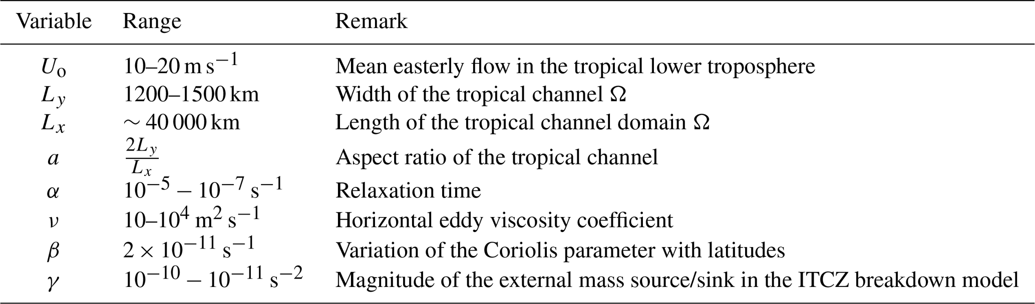
where L_y is the half-width of the tropical channel and L_x is the zonal length of the channel. This domain roughly represents a region where the ITCZ can be treated as a long band wrapping around the Equator. For the current Earth condition, L_x∼40 000 km, and L_y∼1000–1500 km (i.e., 10–15^∘), and so by definition L_x≫L_y.

Table 1 Parameters of the model.

Before we can analyze the ITCZ breakdown model, it is necessary to have first an explicit expression for the forcing term F that represents the vertical mass flux within the ITCZ. In the early study by Ferreira and Schubert (1997), F is a mass source that is a piecewise unit step function of latitudes. To account for the existence of the zonal jet in mid-latitude regions, Legras and Ghil (1985), however, used a forcing of the form $F=\mathit{\alpha }\mathrm{\nabla }{\mathit{\psi }}^{*}$, where ψ^* is a given streamfunction that represents the zonal jet around 50^∘ N. Given our focus on the ITCZ dynamics, we will choose this forcing term such that its corresponding steady state can best represent the typical background flow in the tropical lower troposphere. A zonally symmetric functional form for the F that meets this requirement is

$$\begin{array}{}\text{(3)}& {\displaystyle }F=\mathit{\gamma }\sin {\displaystyle \frac{\mathit{\pi }y}{L_y}},\end{array}$$

where γ denotes the strength of the forcing. Note that this forcing amplitude is not arbitrary, because its value dictates the zonal mean flow in the tropical region as will be shown below.

While the forcing term given by Eq. (3) differs from the unit step function in Ferreira and Schubert (1997), it turns out that Eq. (3) allows a steady solution consistent with the typical flow associated with the ITCZ. Indeed, the steady-state solution ψ_S of Eq. (1) that results from this zonally symmetric forcing is

$$\begin{array}{}\text{(4)}& {\displaystyle }{\mathit{\psi }}_{\mathrm{S}}={\displaystyle \frac{-\mathit{\gamma }{L}_y^{\mathrm{4}}}{{\mathit{\nu }}_{\mathrm{e}}{\mathit{\pi }}^{\mathrm{4}}+\mathit{\alpha }{L}_y^{\mathrm{2}}{\mathit{\pi }}^{\mathrm{2}}}}\sin {\displaystyle \frac{\mathit{\pi }y}{L_y}}.\end{array}$$

The horizontal flow corresponding to this steady streamfunction is illustrated in Fig. 1, which shows an easterly flow to the north and a westerly flow to the south of an ITCZ during a typical Northern Hemisphere summer as expected.

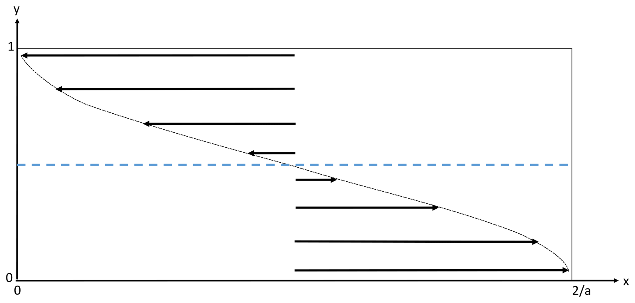
Figure 1 Illustration of the zonal wind that is derived from the steady-state flow ψ_S in the ITCZ model (Eq. 1) with the external forcing given by Eq. (3). The dotted curve represents the horizontal profile of the mean flow, while the black arrows represent the direction of the mean flow for the tropical channel domain Ω_a. The blue dashed line denotes the location of the ITCZ.

Given the above forcing F and its corresponding steady state, the problem of the ITCZ breakdown is now mathematically reduced to the study of the stability of the steady state (Eq. 4) as the model parameters vary. To this end, it is more convenient to rewrite Eq. (1) in the nondimensional form such that our subsequent mathematical analyses can be simplified. Given the governing Eq. (1), it is apparent that the natural scaling for time, streamfunction, and distance can be chosen respectively as follows:

$$\begin{array}{rl}& t={\displaystyle \frac{\mathrm{1}}{L_y\mathit{\beta }}}{t}^{*},\mathit{\psi }=L_y{U}_{\mathrm{0}}{\mathit{\psi }}^{*},(x,y)=L_y(x^{*},y^{*}),\\ & F={\displaystyle \frac{\mathit{\alpha }{U}_{\mathrm{0}}}{L_y}}{F}^{*},\end{array}$$

where the asterisk denotes the nondimensional variables, and U₀ is a given characteristic horizontal velocity that determines the strength of the zonal mean flow in the tropical region. Nondimensionalizing Eq. (1) and neglecting the asterisks hereinafter, the nondimensional form for Eq. (1) becomes

$$\begin{array}{}\text{(5)}& {\displaystyle \frac{\partial \mathrm{\Delta }\mathit{\psi }}{\partial t}}+\mathit{ϵ}J(\mathit{\psi },\mathrm{\Delta }\mathit{\psi })={\displaystyle }E{\mathrm{\Delta }}^{\mathrm{2}}\mathit{\psi }+F-A\mathrm{\Delta }\mathit{\psi }-{\displaystyle \frac{\partial \mathit{\psi }}{\partial x}},\end{array}$$

where

$$\begin{array}{rl}& \mathit{ϵ}={\displaystyle \frac{U_{\mathrm{0}}}{L_y^{\mathrm{2}}\mathit{\beta }}}\text{is the Rossby number,}\\ & E={\displaystyle \frac{{\mathit{\nu }}_{\mathrm{e}}}{L_y^{\mathrm{3}}\mathit{\beta }}}\text{is the Ekman number, and}\\ & A={\displaystyle \frac{\mathit{\alpha }}{L_y\mathit{\beta }}}\text{is the ratio of the relaxation time to the inherent}\\ & \text{time related to the Earth's rotation rate}.\end{array}$$

For the sake of mathematical convenience, we will hereinafter extend the domain from [0,L_y] to $[-L_y,L_y]$ such that the boundary conditions become meridionally symmetric along the Equator at y=0. This mathematical extension of the domain will simplify many calculations, while it has no effect on our solutions so long as we limit the final solution in the original domain $[\mathrm{0},L_x]\times [\mathrm{0},L_y]$ and maintain the Neumann boundary at y=0 as shown below. The nondimensionalized domain is therefore given by

$${\displaystyle }\mathrm{\Omega }=\left[\mathrm{0},{\displaystyle \frac{\mathrm{2}}{a}}\right]\times \left[-\mathrm{1},\mathrm{1}\right],$$

where the scale factor $a\equiv \mathrm{2}{L}_y/L_x$ is introduced to simplify our spectral analyses. Given the above nondimensionlization, the nondimensional form of the forcing (Eq. 3) is now simply

$$\begin{array}{}\text{(6)}& {\displaystyle }F={\mathit{\gamma }}_{\mathrm{1}}\sin \mathit{\pi }y,\end{array}$$

where the nondimensional parameter ${\mathit{\gamma }}_{\mathrm{1}}=\frac{\mathit{\gamma }L}{\mathit{\alpha }{U}_{\mathrm{0}}}$ denotes the ratio of the forcing amplitude γ to the response U₀, and the nondimensional form of the steady state (Eq. 4) is

$$\begin{array}{}\text{(7)}& {\displaystyle }{\displaystyle }{\mathit{\psi }}_{\mathrm{S}}=-{\displaystyle \frac{A{\mathit{\gamma }}_{\mathrm{1}}}{E{\mathit{\pi }}^{\mathrm{4}}+A{\mathit{\pi }}^{\mathrm{2}}}}\sin \mathit{\pi }y.\end{array}$$

We examine next the stability of the steady state (Eq. 7) and how this critical point would bifurcate into different states as the model parameters vary, using Ma and Wang's dynamical transition framework (Ma and Wang, 2013). To this end, it is necessary to study the behaviors of a perturbation ψ^′ around the given steady state (Eq. 4) in the form $\mathit{\psi }={\mathit{\psi }}_{\mathrm{S}}+{\mathit{\psi }}^{\prime }$. This step is not an approximation but simply shifts the location of the stability analyses to the equilibrium ψ_S, much like shifting the coordinate origin from 0 to a new critical point in any linear stability analyses. Note that in Ma and Wang's dynamical transition framework, the full nonlinearity is maintained such that the analyses on the central manifold can be subsequently carried out. Thus, no assumption of ${\mathit{\psi }}^{\prime }\ll {\mathit{\psi }}_{\mathrm{S}}$ is needed for the dynamical transition. With this partition, the corresponding governing equation for the perturbation ψ^′ then becomes

$$\begin{array}{}\text{(8)}& \begin{array}{rl}{\displaystyle \frac{\partial \mathrm{\Delta }\mathit{\psi }}{\partial t}}& +\mathit{ϵ}J(\mathit{\psi },\mathrm{\Delta }\mathit{\psi })=E{\mathrm{\Delta }}^{\mathrm{2}}\mathit{\psi }-A\mathrm{\Delta }\mathit{\psi }-{\displaystyle \frac{\partial \mathit{\psi }}{\partial x}}\\ & +R{\displaystyle \frac{d{\stackrel{\mathrm{̃}}{\mathit{\psi }}}_{\mathrm{S}}}{\mathrm{d}y}}{\displaystyle \frac{\partial \mathrm{\Delta }\mathit{\psi }}{\partial x}}-R{\displaystyle \frac{d^{\mathrm{3}}\stackrel{\mathrm{̃}}{{\mathit{\psi }}_S}}{\mathrm{d}{y}^{\mathrm{3}}}}{\displaystyle \frac{\partial \mathit{\psi }}{\partial x}},\end{array}\end{array}$$

where all the primes are hereinafter omitted for the sake of convenience, and a nondimensional number R and $\stackrel{\mathrm{̃}}{{\mathit{\psi }}_{\mathrm{S}}}$ are defined as follows.

$$\begin{array}{}\text{(9)}& R={\displaystyle \frac{{\mathit{\gamma }}_{\mathrm{1}}\mathit{ϵ}}{E{\mathit{\pi }}^{\mathrm{3}}+A\mathit{\pi }}},\stackrel{\mathrm{̃}}{{\mathit{\psi }}_{\mathrm{S}}}=-{\displaystyle \frac{\sin \mathit{\pi }y}{\mathit{\pi }}}.\end{array}$$

Physically, the nondimensional number R is a ratio between the external forcing amplitude γ₁ and the sum of the viscous and linear damping terms. As will be shown below, this number turns out to be a key bifurcation parameter that determines the dynamical transition of the ITCZ breakdown model.

Given the nature of the ITCZ model, the periodic boundary conditions will be then imposed in the zonal direction, and the free boundary conditions in the meridional direction for the perturbation Eq. (8) are applied at $y=-\mathrm{1}$ and y=1 such that

$$\begin{array}{}\text{(10)}& {\displaystyle }\begin{array}{rl}{\displaystyle }& {\displaystyle }\mathit{\psi }(t,\mathrm{0},y)=\mathit{\psi }\left(t,{\displaystyle \frac{\mathrm{2}}{a}},y\right),\\ {\displaystyle }& {\displaystyle }\mathit{\psi }(t,x,-\mathrm{1})=\mathit{\psi }(t,x,\mathrm{1})=\mathrm{0},and\\ {\displaystyle }& {\displaystyle \frac{{\partial }^{\mathrm{2}}\mathit{\psi }}{\partial y^{\mathrm{2}}}}(t,x,-\mathrm{1})={\displaystyle \frac{{\partial }^{\mathrm{2}}\mathit{\psi }}{\partial y^{\mathrm{2}}}}(t,x,\mathrm{1})=\mathrm{0}.\end{array}\end{array}$$

The periodic boundary conditions along the west–east direction are naturally expected because of the cyclic property of the tropical channel around the Equator, while the free boundary conditions along the south–north direction will ensure that there is no meridional exchange (i.e., no v-wind component) at $y=-\mathrm{1}$ and y=1. Apparently, the Neumann boundary condition at y=0 is still valid after the domain extension because of the continuity of the solution at y=0 in the interior region.

To further reduce the governing equation of the perturbation as given by Eq. (8), we rewrite Eq. (8) in terms of an abstract functional notation that is standard in the study of the nonlinear dynamical transition. Three differential operators ℒ, 𝒢, and 𝒜 are introduced as follows.

$$\begin{array}{ll}\text{(11)}& {\displaystyle }& {\displaystyle }\mathcal{A}\mathit{\psi }\equiv \mathrm{\Delta }\mathit{\psi },{\displaystyle }& {\displaystyle }\mathcal{L}\mathit{\psi }\equiv E{\mathrm{\Delta }}^{\mathrm{2}}\mathit{\psi }-A\mathrm{\Delta }\mathit{\psi }-{\displaystyle \frac{\partial \mathit{\psi }}{\partial x}}+R{\displaystyle \frac{d\stackrel{\mathrm{̃}}{{\mathit{\psi }}_S}}{\mathrm{d}y}}{\displaystyle \frac{\partial \mathrm{\Delta }\mathit{\psi }}{\partial x}}\\ \text{(12)}& {\displaystyle }& {\displaystyle }-R{\displaystyle \frac{d^{\mathrm{3}}\stackrel{\mathrm{̃}}{{\mathit{\psi }}_S}}{\mathrm{d}{y}^{\mathrm{3}}}}{\displaystyle \frac{\partial \mathit{\psi }}{\partial x}},\text{(13)}& {\displaystyle }& {\displaystyle }\mathcal{G}\mathit{\psi }\equiv \mathit{ϵ}J(\mathrm{\Delta }\mathit{\psi },\mathit{\psi }).\end{array}$$

Physically, ℒ is the Laplacian operator, 𝒢 is a linear operator that contains the advection associated with the background flow, and 𝒜 is a nonlinear operator representing the Jacobian effect. Equation (8) for the perturbation streamfunction with boundary condition (Eq. 10) can be then put into the following abstract operator form.

$$\begin{array}{}\text{(14)}& {\displaystyle \frac{\partial \mathcal{A}\mathit{\psi }}{\partial t}}=\mathcal{L}\mathit{\psi }-\mathcal{G}\left(\mathit{\psi }\right).\end{array}$$

As seen in this abstract form, the operators 𝒜 and ℒ are linear, whereas 𝒢 is a nonlinear operator due to the Jacobian's term. A typical analysis of Eq. (14) is to examine first the spectra of eigenvalues and eigenvectors of the linear component ℒ. We then determine the stability characteristics of the linear system, and finally construct the central manifold function with the full nonlinear terms included so that the stable and/or unstable properties of the new states of Eq. (8) can be quantified as the model parameters vary. The outcomes from these analyses are (i) the conditions in the large-scale environment that could determine the stability of the steady state as well as the upper bound on the number of unstable disturbances, and (ii) the structure of new states after the dynamical transition that the large-scale flows must possess to allow for the formation of initial tropical disturbances. These outcomes are important, because they could allow us to quantify the maximum number of environmental tropical embryos that the ITCZ can support in the tropical channel, thus addressing the question of the maximum number TCs that we would expect in the tropical region at any given time.

3 An upper bound on unstable modes

3.1 Eigenmode analyses

We start first with the search for the entire spectrum of the eigenvalues ρ of the linear operator ℒ in Eq. (14). A linear operator L(ρ) is defined as follows:

$$\begin{array}{}\text{(15)}& {\displaystyle }L\left(\mathit{\rho }\right)\mathit{\psi }{\displaystyle }=\mathcal{L}\mathit{\psi }-\mathit{\rho }\mathit{\psi },\mathit{\rho }\in \mathbb{C}.\end{array}$$

Then, all eigenvectors of the linear operator ℒ are nontrivial solutions of L(ρ)ψ=0 with the corresponding eigenvalue ρ. Because of the periodic boundary condition in the x direction, it turns out that the eigenvectors cannot be arbitrary. Indeed, the boundary conditions (Eq. 10) impose a strict constraint on the possible functional forms of ψ such that every eigenvector ψ of ℒ must be expressed in the following separable form.

$$\begin{array}{}\text{(16)}& {\displaystyle }{\mathit{\psi }}_m(x,y)=e^{i\mathit{\pi }\max }\mathrm{\Psi }\left(y\right),\end{array}$$

where m∈ℤ is any integer representing the zonal eigenmodes, and Ψ(y) is the perturbation amplitude. Denoting the corresponding eigenvalue ρ_m for each meridional mode m, a substitution of the preceding separable form into the eigenvalue equation L(ρ_m)ψ=0 yields

$$\begin{array}{}\text{(17)}& {\displaystyle }\left\{\begin{array}{l}{\mathcal{L}}_m\mathrm{\Psi }={\mathit{\rho }}_m{\mathcal{A}}_m\mathrm{\Psi },\\ \mathrm{\Psi }(-\mathrm{1})=\mathrm{\Psi }\left(\mathrm{1}\right)={\mathrm{\Psi }}^{\prime \prime }(-\mathrm{1})={\mathrm{\Psi }}^{\prime \prime }\left(\mathrm{1}\right)=\mathrm{0},\end{array}\right.\end{array}$$

where each prime in Eq. (17) hereinafter denotes a derivative of the streamfunction with respect to y, and the following notations have been introduced:

$$\begin{array}{}\text{(18)}& {\displaystyle }& {\displaystyle }\begin{array}{rl}{\displaystyle }& {\displaystyle }{\mathcal{L}}_m\mathrm{\Psi }\equiv E(D^{\mathrm{2}}-a^{\mathrm{2}}{m}^{\mathrm{2}}{\mathit{\pi }}^{\mathrm{2}}{)}^{\mathrm{2}}\mathrm{\Psi }-A(D^{\mathrm{2}}-a^{\mathrm{2}}{m}^{\mathrm{2}}{\mathit{\pi }}^{\mathrm{2}})\mathrm{\Psi }-\\ {\displaystyle }& {\displaystyle }ima\mathit{\pi }\mathrm{\Psi }+ima\mathit{\pi }R{\stackrel{\mathrm{̃}}{\mathit{\psi }}}_{\mathrm{S}}^{\prime }(D^{\mathrm{2}}-a^{\mathrm{2}}{m}^{\mathrm{2}}{\mathit{\pi }}^{\mathrm{2}})\mathrm{\Psi }\\ {\displaystyle }& {\displaystyle }-ima\mathit{\pi }R{\stackrel{\mathrm{̃}}{\mathit{\psi }}}_{\mathrm{S}}^{\prime \prime \prime }\mathrm{\Psi },\end{array}\text{(19)}& {\displaystyle }& {\displaystyle }{\mathcal{A}}_m\mathrm{\Psi }=(D^{\mathrm{2}}-a^{\mathrm{2}}{m}^{\mathrm{2}}{\mathit{\pi }}^{\mathrm{2}})\mathrm{\Psi },\text{and}\text{(20)}& {\displaystyle }& {\displaystyle }D\equiv d/\mathrm{d}y.\end{array}$$

Applying the boundary conditions $\mathrm{\Psi }(-\mathrm{1})=\mathrm{\Psi }\left(\mathrm{1}\right)={\mathrm{\Psi }}^{\prime \prime }(-\mathrm{1})={\mathrm{\Psi }}^{\prime \prime }\left(\mathrm{1}\right)=\mathrm{0}$ to Eq. (17), it can be seen further that all even-order derivatives of the perturbation amplitude Ψ(y) vanish at the boundaries, i.e.,

$$\begin{array}{}\text{(21)}& {\displaystyle }{\mathrm{\Psi }}^{\left(\mathrm{2}n\right)}(-\mathrm{1})={\mathrm{\Psi }}^{\left(\mathrm{2}n\right)}\left(\mathrm{1}\right)=\mathrm{0},n=\mathrm{0},\mathrm{1},\mathrm{\cdots },\end{array}$$

where n represents the order of derivative with respect to the y direction. This important property of the perturbation amplitude Ψ(y) results in a constraint that Ψ(y) must be expressed in the following form.

$$\begin{array}{}\text{(22)}& {\displaystyle }\mathrm{\Psi }\left(y\right)=\sum _{n\ge \mathrm{0}}{\mathit{\varphi }}_n\cos \left(n+{\displaystyle \frac{\mathrm{1}}{\mathrm{2}}}\right)\mathit{\pi }y+\sum _{n\ge \mathrm{1}}{\stackrel{\mathrm{̃}}{\mathit{\varphi }}}_n\sin n\mathit{\pi }y,\end{array}$$

where ϕ_n and ${\stackrel{\mathrm{̃}}{\mathit{\varphi }}}_n$ are the coefficients to be determined by the eigenvalue equation. As a result, every solution ψ_m(x,y) of L(ρ)ψ=0 can be expressed as

$$\begin{array}{}\text{(23)}& \begin{array}{rl}{\mathit{\psi }}_m(x,y)& =\sum _{n\ge \mathrm{0}}{i}^n{e}^{ima\mathit{\pi }x}{\mathit{\varphi }}_{m,n}\cos \left(n+{\displaystyle \frac{\mathrm{1}}{\mathrm{2}}}\right)\mathit{\pi }y\\ & +\sum _{n\ge \mathrm{1}}{i}^n{e}^{ima\mathit{\pi }x}{\stackrel{\mathrm{̃}}{\mathit{\varphi }}}_{m,n}\sin n\mathit{\pi }y,m\in \mathbb{Z},\end{array}\end{array}$$

where we have redefined the expansion coefficients as iⁿϕ_m,n and $i^n{\stackrel{\mathrm{̃}}{\mathit{\varphi }}}_n$ instead of ϕ_m,n and ${\stackrel{\mathrm{̃}}{\mathit{\varphi }}}_n$ as in Eq. (22) for the sake of convenience.

In what follows, we will determine the wavenumber m such that the eigenvector ψ_m given by Eq. (23) becomes first unstable, i.e., the real part of the corresponding eigenvalue ρ_m becomes positive, as the control parameter R increases. (Requirements for the existence of the first unstable mode are known as the principle of exchange of stabilities (PES) conditions. See Appendix A.) It can be verified that for any complex eigenvalue ρ_m∈ℂ, ψ_m and L(ρ)ψ_m will have the same functional form. Thus, let us denote

$$\begin{array}{}\text{(24)}& \begin{array}{rl}L\left({\mathit{\rho }}_m\right){\mathit{\psi }}_m& =L\left({\mathit{\rho }}_m\right)\sum _{n\ge \mathrm{0}}{i}^n{e}^{ima\mathit{\pi }x}{\mathit{\varphi }}_{m,n}\cos \left(n+{\displaystyle \frac{\mathrm{1}}{\mathrm{2}}}\right)\mathit{\pi }y\\ & +L\left({\mathit{\rho }}_m\right)\sum _{n\ge \mathrm{1}}{i}^n{e}^{ima\mathit{\pi }x}{\stackrel{\mathrm{̃}}{\mathit{\varphi }}}_{m,n}\sin n\mathit{\pi }y\end{array}\end{array}$$

$$\begin{array}{}\text{(25)}& \begin{array}{rl}& \equiv \sum _{n\ge \mathrm{0}}{i}^n{e}^{ima\mathit{\pi }x}{\mathit{\phi }}_{m,n}\cos \left(n+{\displaystyle \frac{\mathrm{1}}{\mathrm{2}}}\right)\mathit{\pi }y\\ & +\sum _{n\ge \mathrm{1}}{i}^n{e}^{ima\mathit{\pi }x}{\stackrel{\mathrm{̃}}{\mathit{\phi }}}_{m,n}\sin n\mathit{\pi }y=\mathrm{0}.\end{array}\end{array}$$

Apparently, Eq. (23) is an eigenvector of the eigenvalue equation L(ρ_m)ψ=0 if and only if the above identity is true $\forall (x,y)$. As a result, explicit calculation of each term in Eq. (24) will lead to

$$\begin{array}{ll}{\displaystyle }{\mathit{\phi }}_{m,n}& {\displaystyle }=B_{m,n+\mathrm{1}}{\mathit{\varphi }}_{m,n+\mathrm{1}}+C_{m,n}{\mathit{\varphi }}_{m,n}-B_{m,n-\mathrm{1}}{\mathit{\varphi }}_{m,n-\mathrm{1}}\\ \text{(26)}& {\displaystyle }& {\displaystyle }=\mathrm{0},n\ge \mathrm{1},\end{array}$$

$$\begin{array}{ll}{\displaystyle }{\mathit{\phi }}_{m,\mathrm{0}}& {\displaystyle }=B_{m,\mathrm{1}}{\mathit{\varphi }}_{m,\mathrm{1}}+C_{m,\mathrm{0}}{\mathit{\varphi }}_{m,\mathrm{0}}+i\left(A_{m,\mathrm{0}}{\mathit{\varphi }}_{m,\mathrm{0}}-{\mathit{\varphi }}_{m,\mathrm{0}}\right)\\ \text{(27)}& {\displaystyle }& {\displaystyle }=\mathrm{0},n=\mathrm{0},\end{array}$$

$$\begin{array}{ll}{\displaystyle }{\stackrel{\mathrm{̃}}{\mathit{\phi }}}_{m,n}& {\displaystyle }=D_{m,n+\mathrm{1}}{\stackrel{\mathrm{̃}}{\mathit{\varphi }}}_{m,n+\mathrm{1}}+E_{m,n}{\stackrel{\mathrm{̃}}{\mathit{\varphi }}}_{m,n}-D_{m,n-\mathrm{1}}{\stackrel{\mathrm{̃}}{\mathit{\varphi }}}_{m,n-\mathrm{1}}\\ \text{(28)}& {\displaystyle }& {\displaystyle }=\mathrm{0},n\ge \mathrm{2}\end{array}$$

$$\begin{array}{}\text{(29)}& {\displaystyle }{\stackrel{\mathrm{̃}}{\mathit{\phi }}}_{m,\mathrm{1}}=D_{m,\mathrm{2}}{\stackrel{\mathrm{̃}}{\mathit{\varphi }}}_{m,\mathrm{2}}+E_{m,\mathrm{1}}{\stackrel{\mathrm{̃}}{\mathit{\varphi }}}_{m,\mathrm{1}}=\mathrm{0},n=\mathrm{1},\end{array}$$

where the coefficients $A_{m,n},B_{m,n},C_{m,n},D_{m,n},E_{m,n}$ are

$$\begin{array}{}\text{(30)}& {\displaystyle }& {\displaystyle }\begin{array}{rl}{\displaystyle }& {\displaystyle }\left\{\begin{array}{l}{A}_{m,n}=a^{\mathrm{2}}{m}^{\mathrm{2}}+{\left(n+\mathrm{1}/\mathrm{2}\right)}^{\mathrm{2}}\\ B_{m,n+\mathrm{1}}=(\mathrm{1}-A_{m,n+\mathrm{1}})\\ C_{m,n}=\frac{\mathrm{2}{\mathit{\pi }}^{\mathrm{3}}E{A}_{m,n}^{\mathrm{2}}+\mathrm{2}\mathit{\pi }(A+{\mathit{\rho }}_m)A_{m,n}-\mathrm{2}iam}{am{\mathit{\pi }}^{\mathrm{2}}R}\end{array}\right.,n\ge \mathrm{0},\left|m\right|\ge \mathrm{1},\\ {\displaystyle }& {\displaystyle }\left\{\begin{array}{l}{B}_{\mathrm{0},n+\mathrm{1}}=(\mathrm{1}-A_{\mathrm{0},n+\mathrm{1}})A_{\mathrm{0},n}={\left(n+\mathrm{1}/\mathrm{2}\right)}^{\mathrm{2}}\\ C_{\mathrm{0},n}=\mathrm{2}{\mathit{\pi }}^{\mathrm{3}}E{A}_{\mathrm{0},n}^{\mathrm{2}}+\mathrm{2}\mathit{\pi }(A+{\mathit{\rho }}_m)A_{\mathrm{0},n}\end{array}\right.,n\ge \mathrm{0},m=\mathrm{0},\end{array}\text{(31)}& {\displaystyle }& {\displaystyle }\begin{array}{rl}{\displaystyle }& {\displaystyle }\left\{\begin{array}{l}{D}_{m,n}=(\mathrm{1}-{\stackrel{\mathrm{̃}}{A}}_{m,n}),{\stackrel{\mathrm{̃}}{A}}_{m,n}=a^{\mathrm{2}}{m}^{\mathrm{2}}+n^{\mathrm{2}}\\ E_{m,n}=\frac{E{\mathit{\pi }}^{\mathrm{3}}{\stackrel{\mathrm{̃}}{A}}_{m,n}^{\mathrm{2}}+\mathit{\pi }(A+{\mathit{\rho }}_m){\stackrel{\mathrm{̃}}{A}}_{m,n}-i\mathrm{2}am}{am{\mathit{\pi }}^{\mathrm{2}}R}\end{array}\right.,n\ge \mathrm{1},\left|m\right|\ge \mathrm{1},\\ {\displaystyle }& {\displaystyle }\left\{\begin{array}{l}{D}_{\mathrm{0},n}=(\mathrm{1}-{\stackrel{\mathrm{̃}}{A}}_{\mathrm{0},n}),{\stackrel{\mathrm{̃}}{A}}_{\mathrm{0},n}=n^{\mathrm{2}}\\ E_{\mathrm{0},n}=E{\mathit{\pi }}^{\mathrm{3}}{\stackrel{\mathrm{̃}}{A}}_{\mathrm{0},n}^{\mathrm{2}}+\mathit{\pi }(A+{\mathit{\rho }}_m){\stackrel{\mathrm{̃}}{A}}_{\mathrm{0},n}\end{array}\right.,n\ge \mathrm{1},m=\mathrm{0}.\end{array}\end{array}$$

Given the conditions (26)–(29), a simple way to obtain the amplitudes ϕ_m,n and ${\stackrel{\mathrm{̃}}{\mathit{\varphi }}}_{m,n}$ is to group all coefficients ϕ_m,n in each of these identities. This can be done effectively by multiplying the conjugate coefficient $\stackrel{\mathrm{‾}}{{\mathit{\varphi }}_{m,n}}$ and a factor B_m,n on both sides of Eqs. (26)–(27), and similarly $\stackrel{\mathrm{‾}}{{\stackrel{\mathrm{̃}}{\mathit{\varphi }}}_{m,n}}$ and a factor D_m,n on both sides of Eqs. (28)–(29). Adding the resulting identities together and taking the sum over n allows us to extract a relationship between the amplitudes of ϕ_m,n and the eigenvalue ρ_m as follows:

$$\begin{array}{}\text{(32)}& {\displaystyle }& {\displaystyle }\sum _{n\ge \mathrm{0}}{B}_{m,n}{\mathit{\phi }}_{m,n}\stackrel{\mathrm{‾}}{{\mathit{\varphi }}_{m,n}}=\mathrm{0},\text{(33)}& {\displaystyle }& {\displaystyle }\sum _{n\ge \mathrm{1}}{D}_{m,n}{\stackrel{\mathrm{̃}}{\mathit{\phi }}}_{m,n}\stackrel{\mathrm{‾}}{{\stackrel{\mathrm{̃}}{\mathit{\varphi }}}_{m,n}}=\mathrm{0}.\end{array}$$

Note that all pairs of the form $(B_{m,n+\mathrm{1}}{B}_{m,n}{\stackrel{\mathrm{‾}}{\mathit{\varphi }}}_{m,n+\mathrm{1}}{\mathit{\varphi }}_{m,n},B_{m,n+\mathrm{1}}{B}_{m,n}{\mathit{\varphi }}_{m,n+\mathrm{1}}{\stackrel{\mathrm{‾}}{\mathit{\varphi }}}_{m,n})$ in Eq. (32) are conjugated to each other so that their sum will produce a purely imaginary number. As a result, the real parts of Eqs. (32) and (33) must come from the term involving C_m,n and can be therefore obtained as

$$\begin{array}{}\text{(34)}& {\displaystyle }& {\displaystyle }\sum _{n\ge \mathrm{0}}{B}_{m,n}{A}_{m,n}(E{\mathit{\pi }}^{\mathrm{2}}{A}_{m,n}+A+\mathrm{\Re }[{\mathit{\rho }}_m\left]\right)|{\mathit{\varphi }}_{m,n}{|}^{\mathrm{2}}=\mathrm{0},\text{(35)}& {\displaystyle }& {\displaystyle }\sum _{n\ge \mathrm{1}}{D}_{m,n}{\stackrel{\mathrm{̃}}{A}}_{m,n}(E{\mathit{\pi }}^{\mathrm{2}}{\stackrel{\mathrm{̃}}{A}}_{m,n}+A+\mathrm{\Re }[{\mathit{\rho }}_m\left]\right)|{\stackrel{\mathrm{̃}}{\mathit{\varphi }}}_{m,n}{|}^{\mathrm{2}}=\mathrm{0},\end{array}$$

where ℜ denotes an operator taking a real part of a complex number. By imposing the physical requirement on the existence of the eigenmodes with ${\mathit{\varphi }}_{m,n}\ne \mathrm{0}$ and ${\stackrel{\mathrm{̃}}{\mathit{\varphi }}}_{m,n}\ne \mathrm{0}$, Eqs. (34)–(35) can provide a great insight into the stability and structure of the eigenmodes that we will now turn to.

3.2 Upper bound on the unstable eigenmode

Equations (34)–(35) contain a number of powerful properties. First, note that the real part of the eigenvalue ρ_m for m=0 must be negative, if it exists, due to the properties that the coefficients A>0, $A_{\mathrm{0},n}>\mathrm{0}$, $B_{\mathrm{0},n}\le \mathrm{0}$, and $D_{\mathrm{0},n}\le \mathrm{0}$. Indeed, if we assume that there exists an eigenvector ψ_m such that ℜ[ρ_m]>0 for m=0, then it can be directly seen from the quadratic form of Eq. (34) that

$${\displaystyle }{\mathit{\varphi }}_{\mathrm{0},n}=\mathrm{0},{\stackrel{\mathrm{̃}}{\mathit{\varphi }}}_{\mathrm{0},n}=\mathrm{0},n\ge \mathrm{0},$$

and so no solution would exist at all, which contradicts our assumption of the existence of the eigenvector for m=0. Thus, the zonally symmetric mode with m=0 is always stable. Because this stable mode does not allow us to examine any transition behaviors, this special zonally symmetric mode will not be considered hereafter.

For m≠0, it can be seen also from Eq. (34) that all possible unstable eigenvectors with m≠0 must satisfy the following constraints

$$\begin{array}{}\text{(36)}& {\displaystyle }\left\{\begin{array}{l}\left\{\begin{array}{l}{\mathit{\varphi }}_{m,n}=\mathrm{0},\text{when},a\ge \frac{\sqrt{\mathrm{3}}}{\mathrm{2}},m\in Z;\\ {\mathit{\varphi }}_{m,n}=\mathrm{0},\text{when},\frac{\sqrt{\mathrm{3}}}{\mathrm{4}}\le a<\frac{\sqrt{\mathrm{3}}}{\mathrm{2}},\left|m\right|\ge \mathrm{2},\\ {\mathit{\varphi }}_{m,n}=\mathrm{0},\text{when},\frac{\sqrt{\mathrm{3}}}{\mathrm{6}}\le a<\frac{\sqrt{\mathrm{3}}}{\mathrm{4}},\left|m\right|\ge \mathrm{3},\\ \mathrm{\cdots }\mathrm{⋮}\mathrm{\cdots }\\ {\mathit{\varphi }}_{m,n}=\mathrm{0},\text{when},\frac{\sqrt{\mathrm{3}}}{\mathrm{2}k}\le a<\frac{\sqrt{\mathrm{3}}}{\mathrm{2}k-\mathrm{2}},\left|m\right|\ge k\end{array}\right.\\ {\stackrel{\mathrm{̃}}{\mathit{\varphi }}}_{m,n}=\mathrm{0},n\ge \mathrm{1},\text{for all}a>\mathrm{0}.\end{array}\right.\end{array}$$

These constraints can be explicitly verified if we note again that the condition (Eq. 36) will ensure that the coefficients $A_{m,n}>\mathrm{0}$ and $B_{m,n}<\mathrm{0}$. If we assume that there exists any unstable eigenvector ψ_m with some zonal wavenumber m≠0 such that the corresponding eigenvalue ρ_m satisfies ℜ[ρ_m]>0, then Eq. (34) immediately indicates that ${\mathit{\varphi }}_{m,n}=\mathrm{0},\forall \left|m\right|\ge k$ and $n\in {\mathbb{Z}}^{+}\cup \mathit{\left\{}\mathrm{0}\mathit{\right\}}$ (i.e., ψ_m=0), and so no such unstable eigenvector ψ_m can exist at all. Therefore, we obtain the remarkable result that any possible unstable modes must be bounded by the condition $\left|m\right|\le k$, where k is an integer satisfying the following relationship:

$$\begin{array}{}\text{(37)}& {\displaystyle \frac{\sqrt{\mathrm{3}}}{\mathrm{2}k}}\le a<{\displaystyle \frac{\sqrt{\mathrm{3}}}{\mathrm{2}k-\mathrm{2}}}.\end{array}$$

To help understand the significance of this result, consider a tropical channel domain between 10^∘ S and 10^∘ N in the Earth's atmosphere (i.e., L_y∼1200 km) and L_x∼40 000 km such that $a\equiv \mathrm{2}{L}_y/L_x\approx \mathrm{0.06}$. Using the condition $\frac{\sqrt{\mathrm{3}}}{\mathrm{2}k}\le a<\frac{\sqrt{\mathrm{3}}}{\mathrm{2}k-\mathrm{2}}$, one obtains an upper bound zonal wavenumber k=12. For the current Earth's tropical atmosphere, this upper bound m≤12 appears to be consistent with the most unstable mode m=13, obtained from the idealized simulations by Ferreira and Schubert (1997). In particular, it can be further seen from the constraint (Eq. 37) that a narrower tropical channel width (i.e., smaller L_y) would lead to a smaller aspect ratio a, and so a higher upper bound k. In this regard, our result could offer further insight into how the upper bound in the unstable zonal wavenumber varies on different planets or in different climates with potentially different values of the aspect ratio a. It should be mentioned that the constraint (Eq. 37) does not allow us to know in advance exactly which wavenumber m<k will become first unstable, because the condition $\left|m\right|<k$ includes a range of m whose real part ℜ[ρ_m] could be positive. Nonetheless, the above result is still very significant due to its explicit indication that the unstable wavenumbers cannot be arbitrary but must be upper bounded. Any eigenvectors with $\left|m\right|\ge k$ must be stable and cannot grow.

A natural consequence of the above result is that not only the total number of TC disturbances has an upper limit, but the size of these disturbances must also be limited (i.e., the size of each disturbance is $\sim L_x/m$). If we assume that each of these disturbances could be eventually responsible for one TC embryo, the upper limit in the number of the disturbances as found from the above condition would imply a lower bound on the overall size of TCs, which has to be larger than 3000 km in diameter. That is, the TC size on our current Earth's atmosphere cannot be arbitrarily small, but must be larger than a limit of ∼10³ km, a fact that has been long observed but not fully explained so far. Of course, this TC size implication by no means eliminates the existence of a small TC such as midgets at the higher latitudes, because our analytical results provide only an estimate for the size of an area where a TC disturbance can emerge. Determining the actual size of a fully developed TC requires, however, various complex factors beyond the scope of the TC genesis that is presented in this study (e.g., Chavas et al., 2016).

We emphasize here that the condition on the unstable modes derived from the eigenvalue ℜ[ρ_m] as seen from Eq. (36) is just a necessary condition, and it is by no means sufficient to specifically know which zonal wavenumber in the range of [1,k] will become first unstable. Thus, it is necessary to examine how the real part of the eigenvalue ℜ[ρ_m] varies as the model parameter R increases for each value of m. Note that the nondimensional number R encodes several important large-scale conditions including the Rossby number, the Ekman number, and the strength of the background flow U₀ as seen in Eq. (9). As these large-scale conditions change, R will vary as well. Depending on how the eigenvalue ρ_m varies as a function of R, there may emerge a first unstable zonal wavenumber m with a positive eigenvalue ℜ[ρ_m] that we need to quantify.

To ensure the existence of such a positive eigenvalue as R increases, one needs to show that ℜ[ρ_m] must be an increasing function of R such that the real part can become positive as R increases. The specific wavenumber m for which ℜ[ρ_m] first becomes positive will possess the structure that dictates the new dynamical transition of the system according to the PES conditions. Due to the complication in deriving the exact expression for ρ_m, details of the derivations of ℜ[ρ_m] as a function of R are provided in Appendix 2. An important conclusion from these derivations is that ${lim}_{R\to +\mathrm{\infty }}\mathrm{\Re }\left[{\mathit{\rho }}_m\right(R\left)\right]=+\mathrm{\infty }$, which implies that there indeed exists a critical value R^* at which $\mathrm{\Re }\left[{\mathit{\rho }}_m\right]\left(R^{*}\right)=\mathrm{0}$. This requirement is critical, since it directly indicates that the PES conditions are ensured. More strictly speaking, this result means that there exists a positive integer n≤k and a critical number $R^{*}>\mathrm{0}$ such that the following PES conditions,

$$\begin{array}{}\text{(38)}& \left\{\begin{array}{l}\mathrm{\Re }\left[{\mathit{\rho }}_{n,\mathrm{1}}\right]=\mathrm{\Re }\left[{\mathit{\rho }}_{-n,\mathrm{1}}\right]\left\{\begin{array}{ll}>\mathrm{0}& \text{ if }R>R^{*},\\ =\mathrm{0}& \text{ if }R=R^{*},\forall n=m_{\mathrm{1}},,\mathrm{\cdots },m_l\\ <\mathrm{0}& \text{ if }R<R^{*},\end{array}\right.,\\ \mathrm{\Re }\left[{\mathit{\rho }}_{m,k}\right]<\mathrm{0},\text{ if }(m,k)\ne (m_i,\mathrm{1}),\mathrm{1}\le i\le l,\\ \mathrm{\Im }\left[{\mathit{\rho }}_{n,\mathrm{1}}\right(R\left)\right]\ne \mathrm{0}\text{for}R\ge R^{*},\end{array}\right.\end{array}$$

must hold true. Corresponding to the first unstable mode m and eigenvalue ρ_m,1, its eigenvector is then given by

$${\displaystyle }{\mathit{\psi }}_m=\sum _{n=\mathrm{0}}^{\mathrm{\infty }}{i}^n{e}^{ima\mathit{\pi }x}{\mathit{\varphi }}_{m,n}\cos \left(n+{\displaystyle \frac{\mathrm{1}}{\mathrm{2}}}\right)\mathit{\pi }y,\mathrm{1}\le \left|m\right|\le k.$$

Note that these eigenvectors are unstable for $\left|m\right|<k$ only, because all other eigenvectors $\left(\right|m|>k)$ are always stable as shown by the condition (Eq. 36).

Due to the complicated expression for the eigenvalue ρ_m(R) as shown in Appendix 2, the value R^* cannot be exactly derived but must be numerically approximated for each m. The proof of ${lim}_{R\to +\mathrm{\infty }}\mathrm{\Re }\left[{\mathit{\rho }}_m\right(R\left)\right]=+\mathrm{\infty }$ provided in Appendix 2 ensures that R^* always exists, and so it should be found numerically. Figure 2 shows the critical value $R_m^{*}$ as a function of 2∕a for each value of m, which is obtained by using a numerical approximation. Recall that for each value of a, there will exist only one value k that satisfies $\frac{\sqrt{\mathrm{3}}}{\mathrm{2}k}\le a<\frac{\sqrt{\mathrm{3}}}{\mathrm{2}k-\mathrm{2}}$ and a value m<k such that $\mathrm{\Re }\left[{\mathit{\rho }}_{m,\mathrm{1}}\right]=\mathrm{0}$. By searching for the value of $R_m^{*}$ that ensures $\mathrm{\Re }\left[{\mathit{\rho }}_{m,\mathrm{1}}\right]=\mathrm{0}$, we obtain for each m≤k a curve $R_m^{*}=R_m^{*}\left(a\right)$ that determines the onset of the dynamical transition. Because the eigenvalues and the eigenfunctions corresponding to −m are the complex conjugate of the respective eigenvalues and the eigenfunctions corresponding to m, only the cases of nonnegative m need to be examined.

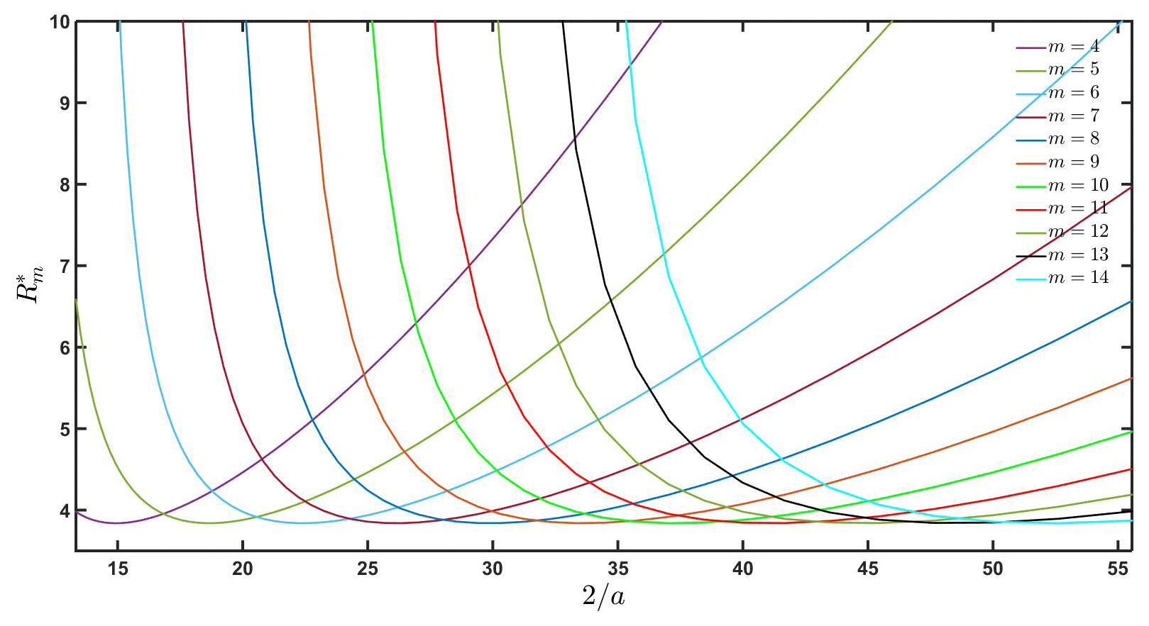
Figure 2 Marginal stability curves $R_m^{*}\left(a\right)$ obtained from the constraint on the eigenvalue $\mathrm{\Re }{\mathit{\rho }}_{m,\mathrm{1}}\left(R\right)=\mathrm{0}$ for a range of the aspect ratio $\mathrm{0.1}\le a\le \mathrm{0.35}$.

As shown in Fig. 2, there are several key differences between the asymptotic limits of a very small and a very large a. Specifically, for a larger value of a (i.e., a wider tropical region), the smaller wavenumbers m will become unstable first, starting with m=5, and then decrease for a larger R. For the smaller value of a (i.e., a narrower tropical channel), the larger wavenumbers will, however, become unstable first as shown in Fig. 2. For example, for the typical scales of the Earth's tropical region with L_x≈40 000 km, and L_y≈1200 km, $\mathrm{2}/a=L_x/|L_y\approx \mathrm{33.3}$. According to Fig. 2, the wavenumber m=9 will become unstable first as R crosses the value $R^{*}=\mathrm{4}$. Thus, the dynamical transition for m=9 will produce a new unstable wave structure corresponding to m=9 at the bifurcation point. As the parameter R increases, other unstable modes corresponding to $m=\mathrm{8},\mathrm{7},\mathrm{6}\mathrm{\dots }$ start to emerge, thus producing a spectrum of unstable structures as a result of the dynamical transition.

To focus on how the first unstable mode changes with the aspect ratio a instead of the critical number R^* as shown in Fig. 2, Fig. 3 shows the first unstable mode m as a function of a, assuming all of the same parameter values used in Fig. 2. It can be seen in this Fig. 3 that for each value of a, there is only one wavenumber n=n(a) for which $R_n^{*}={min}_{m\in \mathbb{N}}{R}_m^{*}$. This is the critical value $R^{*}=R_n^{*}$ at which the dynamical transition will occur according to the PES conditions. Apparently, one can better see in this figure how the first unstable mode depends on the aspect ratio of the tropical channel, with a higher wavenumber for a narrower tropical region. The same behavior is also valid for a range of values of the Ekman number E and Rossby number ϵ, which are not shown here because they do not provide any further information.

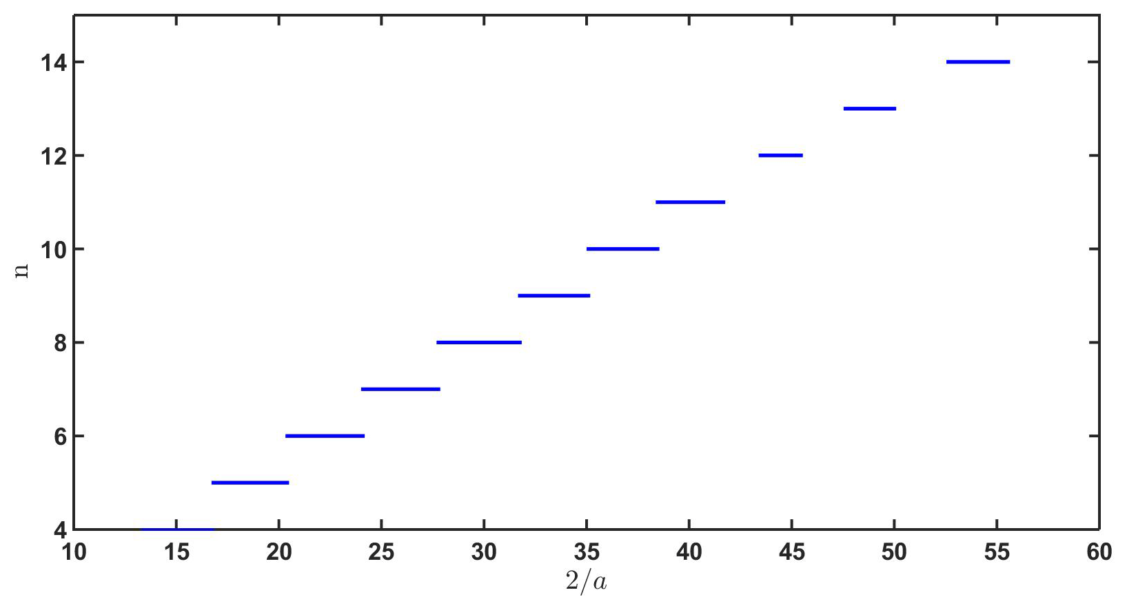
Figure 3 The dependence of the first critical wave number m=n on the scale factor a, assuming the Rossby number ϵ=0.5 and the Ekman number E=0.05 similar to Fig. 2.

4 Bifurcation structure

While the stability analyses in the previous section could show an upper bound on possible unstable modes, the structure of these unstable modes as well as the subsequent effects of the nonlinear terms have not been discussed. The existence of an eigenvalue with a zero real part at $R=R^{*}$ immediately imposes the condition that the stability analyses must require all nonlinear terms so that the behaviors of dynamical transitions can be captured. Depending on the multiplicity of the eigenvalues when the PES conditions are met, one can, however, reduce the full nonlinear system (Eq. 14) to a set of ordinary differential equations on a central manifold at $R=R^{*}$ and construct a central manifold function to examine the bifurcation and the structure of new states with all nonlinear terms included. Standard procedures of stability analyses on the central manifold for the ITCZ model show that there exists indeed a supercritical Hopf bifurcation for $R>R^{*}$, with a new stable state approximated as follows (see Ma and Wang, 2013),

$$\begin{array}{}\text{(39)}& {\displaystyle }\mathit{\psi }={\mathit{\psi }}_S+{\left({\displaystyle \frac{\mathrm{\Re }\left({\mathit{\rho }}_{n,\mathrm{1}}\right)}{\left|\mathrm{\Re }\right(A\left)\right|}}\right)}^{\frac{\mathrm{1}}{\mathrm{2}}}{f}_n(x,y,t)+h.o.t.,\end{array}$$

where h.o.t. denotes higher order terms, provided that the nondimensional parameter R is sufficiently close to R^*, i.e.,

$${\displaystyle }\mathrm{0}<{\displaystyle \frac{R-R^{*}}{R^{*}}}\ll \mathrm{1}.$$

Using a higher-order approximation around the critical point on the extended central manifold, one can obtain a better manifold function that better approximates ψ for $R>R^{*}$. Nonetheless, the smooth behaviors of the eigenvector at $R=R^{*}$ for the supercritical Hopf bifurcation suffices to indicate that the structure of the solution at $R=R^{*}$ can represent well the behavior of the new stable solution near $R=R^{*}$ as dictated by the dynamical transition theorem in Ma and Wang (2013). Technically, either Hopf bifurcation or double Hopf bifurcation may appear, depending on the transition multiplicity at the critical value. This subtlety will introduce much more complex analysis of the bifurcation and transversal intersections of the parameter planes that we will not present herein.

While these higher-order derivations of the central manifold function require some technical details that are beyond the scope of this study, it is possible to approach the transition dynamics by numerically solving the eigenvalue problem (Eq. 18). Specifically, we notice that the x dependence can be obtained by simply searching for the first unstable mode m as R approaches the critical value R^*. Using this numerical approach to find the critical value of R^*, the entire spectrum of eigenvectors associated with the potential new stable states after the dynamical transition can be found for each set of large-scale environmental parameters. We note again at this point that the exact mode m at which the eigenvector becomes first unstable is dependent on R as shown in Figs. 2 and 3. The only constraint we can be certain of is that $\left|m\right|<k$. Thus, a new stable mode for $R>R^{*}$ emerged under the case of the supercritical Hopf bifurcation could inherit all structure of a zonal mode $\left|m\right|<k$ at $R=R^{*}$. This numerical approach is powerful, as it allows one to search for not only the critical parameter R^* at which the PES conditions are ensured, but also the structure of new stable states for any value of $R>R^{*}$ after the bifurcation point.

To illustrate the results from this numerical approach, we consider the following set of the large-scale environmental conditions in the typical tropical region:

$${\displaystyle }\begin{array}{rl}& L_y\sim \mathrm{1000}\text{km},U_{\mathrm{0}}\sim \mathrm{10}{\mathrm{m}\mathrm{s}}^{-\mathrm{1}},\mathit{\alpha }\sim {\mathrm{10}}^{-\mathrm{6}}{\mathrm{s}}^{-\mathrm{1}},\\ & \mathit{\beta }\sim {\mathrm{10}}^{-\mathrm{11}}{\mathrm{m}}^{-\mathrm{1}}{\mathrm{s}}^{-\mathrm{1}},\mathit{\nu }=\mathrm{1000}{\mathrm{m}}^{\mathrm{2}}{\mathrm{s}}^{-\mathrm{1}},\end{array}$$

which result in a Rossby number ϵ≈0.5 and an Ekman number E≈0.05. With the further use of Eq. (4) for the steady state and noting that $U_{\mathrm{0}}=\partial {\mathit{\psi }}_S/\partial y$, one then obtains an estimation for the forcing amplitude $\mathit{\gamma }\approx \mathrm{7}\times {\mathrm{10}}^{-\mathrm{10}}{s}^{-\mathrm{2}}$. From the definition of the nondimensional number R, we then get R≈4.8, which is above the critical value $R^{*}\approx \mathrm{4}$ for m=9 as shown in Fig. 2. Thus, the PES conditions are satisfied, and a new stable structure must emerge after the dynamical transition as a consequence of the supercritical Hopf bifurcation. As such, the eigenvalue problem (Eq. 17) can be solved for the first eigenvector and its dual eigenvector, given the value R=4.8. Note that this estimation of R is most sensitive to the strength of the shear flow U₀, the beta effect β, and the scale L_y but not on the diffusion coefficient ν. To some extent, this insensitivity of the dynamical transition on the diffusion is expected, because the large-scale eddy diffusion process is often negligible.

For this numerical method, we use a Legendre–Galerkin method where the unknown fields are expanded using a basis of N polynomials, which are compact-combinations of the Legendre polynomials satisfying the four boundary conditions (Eq. 17; see Shen et al., 2011, for the details of this numerical method). For the convergence of the numerical scheme, N=100 is sufficient. Once the eigenvector problem is solved, a further approximation on the central manifold can be applied so that the stability of new stable states can be examined around the critical point on the central manifold.

Figure 4 shows a new state as a result of the dynamical transition for $R>R^{*}$ under the supercritical Hopf bifurcation case that is obtained from the numerical procedures described above. Among several significant features of this numerical solution, the most noteworthy one is that the new state possesses a large-scale structure consistent with the ITCZ breakdown as observed in the idealized simulations by Ferreira and Schubert (1997). Specifically, the tropical channel contains 10 large-scale disturbances; each has the horizontal scale of about 5000 km and could serve as embryos for the subsequent TC formation. Furthermore, the disturbances in this new state move to the left with a period of T∼3.2116 (i.e., T≈4 d in the physical dimensional unit) as a result of the nonzero imaginary part of the eigenvalues. For different domain configurations such as different planets or future climates with different tropical width, the unstable structure and/or wave speed may be different, and so the maximum number of the TC-favorable disturbances will change as well.

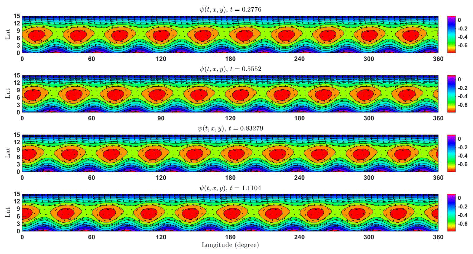
Figure 4 Illustration of the streamfunction ψ for the new periodic state on the central manifold near the critical point R^* after the dynamical transition, assuming ϵ=0.3, E=0.05, and $R=\mathrm{3.8717}>R^{*}=\mathrm{3.8517}$. The nondimensional period is T=2.776, which corresponds to a physical period of ∼3.213 d. Superimposed are corresponding vector flows derived from the streamfunction.

That these large-scale structure of disturbances move to the left with a timescale of ∼4 d as a consequence of the dynamical transition shown above is interesting, because these westward-moving disturbances are to some extent similar to easterly waves in the real atmosphere. While it is entirely possible that these easterly waves are a mode of the equatorial mixed-Rossby waves, it should be noted that the numerical procedure of finding new stable modes on the central manifold presented in this study does not allow us to separate different modes of easterly waves. As such, these easterly waves could be a combination of different modes of westward-moving Rossby waves and mixed-gravity waves that we may not be able to separate. In any case, the easterly waves that are often associated with TC genesis can be now seen as a natural consequence of the dynamical transition, even for barotropic flows. Such a consistency between the observed and theoretical estimation of the large-scale modes in the tropical region suggests that the barotropic instability and its inherent nonlinear dynamics can account for the preconditioning environment for TC genesis.

As a final remark, the large-scale structure shown in Fig. 4 does not itself impose that the disturbances have to grow and turn into TCs. Instead, these structures are simply new stable periodic solutions associated with the supercritical Hopf bifurcation after the dynamical transition occurs. That is, for $R<R^{*}$, the stable structure is the steady state as given in Fig. 2, whereas the new stable structure shown in Fig. 4 will emerge after $R>R^{*}$. As soon as these stable structures emerge, subsequent dynamic-thermodynamic feedback may be triggered and result in further growth of the disturbances within each wave. For a larger value of R, the stability of the periodic state may no longer be ensured, because the central manifold function must be reevaluated and a new structure may arise. The subsequent intensification of any tropical disturbances as a result of the new unstable structure would require additional detailed physics that are, however, not the focus of this work and so will not be discussed hereinafter. In this regard, the new stable periodic state shown in Fig. 4 can serve only as a preconditioning environment for incipient disturbances to grow.

5 Conclusions

In this study, we examined the dynamical mechanisms underlying the large-scale formation of tropical cyclones (TCs) using a barotropic model for the intertropical convergence zone (ITCZ). Assuming a forcing function that mimics the mass sink/source in the ITCZ, it was shown that the large-scale steady flow (i.e., the critical point or equilibrium) in the ITCZ model loses its stability for a bounded range of the wavenumber $\left|m\right|<k$ if large-scale environmental conditions including the magnitude of the mean flow, the Ekman number, and the Rossby number satisfy certain constraints. That the number of the unstable modes in the tropical region is upper bounded is a very significant result, because it could offer an explanation for a fundamental question of why the Earth's tropical atmosphere can support a limited number of TCs globally each year.

Using the principle of exchange of stabilities condition for the ITCZ model, we found that the ITCZ model undergoes a bifurcation with associated dynamical transition at the critical point, which helps determine the maximum number of TC disturbances that the Earth's atmosphere can generate. Specifically, a theoretical estimation of the largest zonal wavenumber k that can allow an unstable structure as a result of the ITCZ breakdown is k=12, assuming the typical scales of the Earth's tropical channel in which the zonal scale of the tropical channel is about an order of magnitude larger than the width of the channel. Such a dynamical constraint on the maximum number of TC disturbances is remarkable, as it suggest an intrinsic large-scale mechanism that controls the climatology of the TC numbers beyond the basin-specific features as recently noted in Patricola et al. (2018). Of interest is that this constraint on the largest wavenumber of the unstable eigenmodes imposes not only an upper limit on the number of TC disturbances in the tropical region, but also a lower bound on the size of TC disturbances. This lower bound on the size of the tropical disturbances may help explain why TCs cannot be arbitrarily small but must be larger than a certain limit in the tropical region.

To verify our theoretical analyses, a numerical method is used to search for the new structure on the central manifold of the ITCZ model as the model parameter R is larger than a critical value R^*. Here, the key parameter R controlling the bifurcation in our ITCZ model is given by

$${\displaystyle }R={\displaystyle \frac{\mathit{\gamma }\mathit{ϵ}\mathit{\pi }}{E{\mathit{\pi }}^{\mathrm{4}}+A{\mathit{\pi }}^{\mathrm{2}}}},$$

where γ is a parameter measuring the strength of the ITCZ mass sink/source, A is the parameter measuring the effect of surface drag, ϵ is a parameter measuring the mean zonal flow, and E is the Ekman number representing the eddy viscosity. Our numerical results confirmed that for $R>R^{*}$, a new large-scale state emerges as a result of the supercritical Hopf bifurcation whose structure depends on the value R. For R sufficiently close to the critical value R^*, the new periodic state possesses a type of wave motion with two groups of symmetric disturbances across the Equator. These new stable periodic solutions describe a type of westward-moving disturbances within the ITCZ, very similar to the classical easterly waves in the tropical region. These findings obtained from the ITCZ breakdown model in this study thus provide new insights into the formation of TC disturbances in the Earth's tropical atmosphere, as well as a rigorous mathematical proof for the bounded number of TCs at the global scale.

Appendix A: Principle of exchange of stabilities

The principle of exchange of stabilities (PES) for a dynamical system basically refers to a critical condition for which the eigenvalues of the linear operator first cross a prescribed value. More precisely, the PES can be precisely stated as follows.

Let L_λ and G represent the linear and nonlinear parts of a dynamical system in the abstract form:

$$\begin{array}{}\text{(A1)}& {\displaystyle \frac{d\mathbf{u}}{\mathrm{d}t}}={\mathbf{L}}_{\mathit{\lambda }}\left(\mathbf{u}\right)+\mathbf{G}(\mathbf{u},\mathit{\lambda }),\end{array}$$

where λ∈ℝ is the model parameter, and u∈ℝⁿ represents the state of the system. By definition, L_λ is a parameterized linear operator that depends continuously on λ. Consider the eigenvalue equation given by

$$\begin{array}{}\text{(A2)}& {\mathbf{L}}_{\mathit{\lambda }}\mathit{e}=\mathit{\beta }\left(\mathit{\lambda }\right)\mathbf{e},\end{array}$$

where e is eigenvector, and β(λ)∈ℂ the eigenvalue. Let ${\mathit{\beta }}_j\left(\mathit{\lambda }\right)\in \mathbb{C}|j\in \mathbb{N}$ be the eigenvalues (counting multiplicity) of L_λ. If we have

$$\begin{array}{}\text{(A3)}& \left\{\begin{array}{l}\mathrm{\Re }\left[{\mathit{\beta }}_j\right(\mathit{\lambda }\left)\right]\left\{\begin{array}{ll}<\mathrm{0}& \text{ if }\mathit{\lambda }<{\mathit{\lambda }}_{\mathrm{0}},\\ =\mathrm{0}& \text{ if }\mathit{\lambda }={\mathit{\lambda }}_{\mathrm{0}},\forall \mathrm{1}\le i\le m\\ >\mathrm{0}& \text{ if }\mathit{\lambda }<{\mathit{\lambda }}_{\mathrm{0}},\end{array}\right.,\\ \mathrm{\Re }\left[{\mathit{\beta }}_j\right({\mathit{\lambda }}_{\mathrm{0}}\left)\right]<\mathrm{0},\forall j\ge m+\mathrm{1},\end{array}\right.\end{array}$$

then the system is said to satisfy the PES condition at λ₀, which signifies a bifurcation of the system from one state to another. For dissipative systems, the PES condition has a much more powerful implication than a simple bifurcation, as it ensures a dynamical transition that can be completely categorized by three different types of transition including the continuous transition, the catastrophic transition, and the random transition. See Ma and Wang (2013) for more details of the PES conditions for nonlinear systems.

Appendix B: Existence of the critical number R^*

For $\frac{\sqrt{\mathrm{3}}}{\mathrm{2}k+\mathrm{2}}\le a<\frac{\sqrt{\mathrm{3}}}{\mathrm{2}k}$ and $\mathrm{1}\le m\le k(k=\mathrm{1},\mathrm{2},\mathrm{\cdots })$, it is easy to see from Eq. (34) that we must have

$${\displaystyle }{\mathit{\varphi }}_{m,\mathrm{0}}\ne \mathrm{0},$$

because otherwise we will have ${\mathit{\varphi }}_{m,n}=\mathrm{0},n\ge \mathrm{0}$, and no eigenvectors would exist. For the sake of convenience, we will hereinafter replace ψ_m by $\frac{{\mathit{\psi }}_m}{B_{m,\mathrm{0}}{\mathit{\varphi }}_{m,\mathrm{0}}}$, and similarly replace ϕ_m,n by $\frac{{\mathit{\varphi }}_{m,n}}{B_{m,\mathrm{0}}{\mathit{\varphi }}_{m,\mathrm{0}}}$. Equations (26)–(27) are then rewritten as follows:

$$\begin{array}{}\text{(B1)}& {\displaystyle }\begin{array}{rl}{\displaystyle }& {\displaystyle }{B}_{m,n+\mathrm{1}}{\mathit{\varphi }}_{m,n+\mathrm{1}}+C_{m,n}{\mathit{\varphi }}_{m,n}-B_{m,n-\mathrm{1}}{\mathit{\varphi }}_{m,n-\mathrm{1}}=\mathrm{0},n\ge \mathrm{1},\\ {\displaystyle }& {\displaystyle }{B}_{m,\mathrm{1}}{\mathit{\varphi }}_{m,\mathrm{1}}+C_{m,\mathrm{0}}{\mathit{\varphi }}_{m,\mathrm{0}}+i\left(A_{m,\mathrm{0}}{\mathit{\varphi }}_{m,\mathrm{0}}-{\mathit{\varphi }}_{m,\mathrm{0}}\right)=\mathrm{0},n=\mathrm{0},\end{array}\end{array}$$

and

$$\begin{array}{}\text{(B2)}& {\displaystyle }{\displaystyle }\sum _{n\ge \mathrm{0}}{B}_{m,n}{A}_{m,n}(E{\mathit{\pi }}^{\mathrm{2}}{A}_{m,n}+A+\mathrm{\Re }[{\mathit{\rho }}_m\left]\right)|{\mathit{\varphi }}_{m,n}{|}^{\mathrm{2}}=\mathrm{0}.\end{array}$$

Denote

$${\displaystyle }{d}_{m,n}={\displaystyle \frac{C_{m,n}}{B_{m,n}}},$$

and let

$${\displaystyle }{\mathit{\eta }}_{m,n}=B_{m,n}{\mathit{\varphi }}_{m,n},$$

and then Eq. (B1) can be further rewritten as

$$\begin{array}{}\text{(B3)}& {\displaystyle }\begin{array}{rl}{\displaystyle }& {\displaystyle }{\mathit{\eta }}_{m,n+\mathrm{1}}+d_{m,n}{\mathit{\eta }}_{m,n}-{\mathit{\eta }}_{m,n-\mathrm{1}}=\mathrm{0},n\ge \mathrm{1},\\ {\displaystyle }& {\displaystyle }{\mathit{\eta }}_{m,\mathrm{1}}+d_{m,\mathrm{0}}-i=\mathrm{0},n\ge \mathrm{0}.\end{array}\end{array}$$

This reduced Eq. (B3) allows us to deduce a number of important constraints. Indeed, we rearrange Eq. (B3) as follows:

$$\begin{array}{}\text{(B4)}& {\displaystyle }\begin{array}{rl}{\displaystyle }& {\displaystyle }-d_{m,\mathrm{0}}+i={\mathit{\eta }}_{m,\mathrm{1}},{\mathit{\eta }}_{m,\mathrm{0}}=\mathrm{1},\\ {\displaystyle }& {\displaystyle }{\mathit{\xi }}_{m,n}={\displaystyle \frac{{\mathit{\eta }}_{m,n}}{{\mathit{\eta }}_{m,n-\mathrm{1}}}}={\displaystyle \frac{\mathrm{1}}{d_{m,n}+\frac{{\mathit{\eta }}_{m,n+\mathrm{1}}}{{\mathit{\eta }}_{m,n}}}},\\ {\displaystyle }& {\displaystyle }-d_{m,\mathrm{0}}+i={\displaystyle \frac{\mathrm{1}}{d_{m,\mathrm{1}}+{\mathit{\xi }}_{m,\mathrm{2}}}}={\displaystyle \frac{\mathrm{1}}{d_{m,\mathrm{1}}+\frac{\mathrm{1}}{d_{m,\mathrm{2}}+{\mathit{\xi }}_{m,\mathrm{3}}}}}.\end{array}\end{array}$$

It is readily seen from Eq. (B3) that ${\mathit{\eta }}_{m,n}=\mathrm{0}$ for all n≥0 whenever there exists a l≥0 for which ${\mathit{\eta }}_{m,l}=\mathrm{0}$. This means that ${\mathit{\xi }}_{m,n}\ne \mathrm{0}$ for all n≥0. From Eq. (B4) one can derive that

$$\begin{array}{}\text{(B5)}& {\displaystyle }{\mathit{\eta }}_{m,n}\equiv {\mathit{\xi }}_{m,\mathrm{1}}{\mathit{\xi }}_{m,\mathrm{2}}\mathrm{\cdots }{\mathit{\xi }}_{m,n},n\ge \mathrm{1}.\end{array}$$

Therefore, for $\frac{\sqrt{\mathrm{3}}}{\mathrm{2}k+\mathrm{1}}\le a<\frac{\sqrt{\mathrm{3}}}{\mathrm{2}k}(k=\mathrm{1},\mathrm{2},\mathrm{3},\mathrm{\dots })$, Eq. (B2) can be equally rewritten as follows:

$$\begin{array}{}\text{(B6)}& {\displaystyle }\left\{\begin{array}{l}\sum _{n\ge \mathrm{0}}\mathrm{\Re }\left[d_{m,n}\right]|{\mathit{\eta }}_{m,n}{|}^{\mathrm{2}}=\mathrm{0},\\ \mathrm{\Re }\left[d_{m,n}\right]<\mathrm{0}(n\ge \mathrm{1}),\mathrm{\Re }\left[d_{m,\mathrm{0}}\right]>\mathrm{0},\end{array}\right.m\le k.\end{array}$$

One can deduce from the third equality of Eq. (B4) that

$$\begin{array}{}\text{(B7)}& {\displaystyle }\begin{array}{rl}{\mathit{\rho }}_m& =-A-{\mathit{\pi }}^{\mathrm{2}}E{A}_{m,\mathrm{0}}\\ & +{\displaystyle \frac{\mathrm{2}iam+iam{\mathit{\pi }}^{\mathrm{2}}R\left(\mathrm{1}-A_{m,\mathrm{0}}\right)}{\mathrm{2}\mathit{\pi }{A}_{m,\mathrm{0}}}}\\ & +{\displaystyle \frac{\frac{-am\mathit{\pi }R\left(\mathrm{1}-A_{m,\mathrm{0}}\right)}{\mathrm{2}{A}_{m,\mathrm{0}}}}{d_{\mathrm{1}}+{\mathit{\xi }}_{m,\mathrm{2}}}}.\end{array}\end{array}$$

Let's define a function F using the right-hand side of Eq. (B7), i.e.,

$${\displaystyle }\begin{array}{rl}F({\mathit{\rho }}_m,R)& =-A-{\mathit{\pi }}^{\mathrm{2}}E{A}_{m,\mathrm{0}}\\ & +{\displaystyle \frac{\mathrm{2}iam+iam{\mathit{\pi }}^{\mathrm{2}}R\left(\mathrm{1}-A_{m,\mathrm{0}}\right)}{\mathrm{2}\mathit{\pi }{A}_{m,\mathrm{0}}}}\\ & +{\displaystyle \frac{\frac{-am\mathit{\pi }R\left(\mathrm{1}-A_{m,\mathrm{0}}\right)}{\mathrm{2}{A}_{m,\mathrm{0}}}}{d_{\mathrm{1}}+{\mathit{\xi }}_{m,\mathrm{2}}}}.\end{array}$$

Due to the fact that

$${\displaystyle }{\displaystyle }\mathrm{\Re }{d}_{m,n}<\mathrm{0}(n\ge \mathrm{1}),$$

we can obtain that

$${\displaystyle }\begin{array}{rl}\left|F\right({\mathit{\rho }}_m,R\left)\right|\le & \left|-A-{\mathit{\pi }}^{\mathrm{2}}E{A}_{m,\mathrm{0}}+{\displaystyle \frac{\mathrm{2}iam+iam{\mathit{\pi }}^{\mathrm{3}}R\left(\mathrm{1}-A_{m,\mathrm{0}}\right)}{\mathrm{2}\mathit{\pi }{A}_{m,\mathrm{0}}}}\right|\\ & +{\displaystyle \frac{\left|\frac{-am\mathit{\pi }R\left(\mathrm{1}-A_{m,\mathrm{0}}\right)}{\mathrm{2}{A}_{m,\mathrm{0}}}\right|}{\left|\mathrm{\Re }\right[d_{\mathrm{1}}\left]\right|}}=K_R.\end{array}$$

Defining a set Ω_R as

$${\displaystyle }{\mathrm{\Omega }}_R=\left\{z\in C\left|\mathrm{\Re }\right[z]>-A-E{\mathit{\pi }}^{\mathrm{2}}\left({\displaystyle \frac{\mathrm{1}}{\mathrm{4}}}+a^{\mathrm{2}}\right),|z|\le K_R\right\},$$

the Brown fixed point theorem implies then that F has a fixed point in Ω_R, i.e., there exists ρ_m(R) such that

$${\displaystyle }{\mathit{\rho }}_m\left(R\right)=F\left({\mathit{\rho }}_m\right(R),R).$$

At last, we prove that ρ_m(R) is a continuous function of R and ℑρ_m(R)≠0. Let G(ρ_m,R) be the function given by

$${\displaystyle }G({\mathit{\rho }}_m,R)=F({\mathit{\rho }}_m,R)-{\mathit{\rho }}_m.$$

If we can prove

$${\displaystyle \frac{\partial G}{\partial {\mathit{\rho }}_m}}\ne \mathrm{0}$$

then the implicit function theorem implies that ρ_m(R) is indeed a continuous function of R. From the definition of G and Eq. (B7), we obtain

$$\begin{array}{ll}{\displaystyle }& {\displaystyle }\left|{\displaystyle \frac{\partial G}{\partial {\mathit{\rho }}_m}}\right|=\left|\sum _{n=\mathrm{1}}(-\mathrm{1}{)}^{n+\mathrm{1}}{\displaystyle \frac{\left(\mathrm{1}-A_{m,\mathrm{0}}\right)A_{m,n}}{A_{m,\mathrm{0}}\left(\mathrm{1}-A_{m,n}\right)}}{\mathit{\eta }}_{m,n}^{\mathrm{2}}({\mathit{\rho }}_m\left(R\right))-\mathrm{1}\right|\\ {\displaystyle }& {\displaystyle }\ge \mathrm{1}-\sum _{n=\mathrm{1}}{\displaystyle \frac{\left(\mathrm{1}-A_{m,\mathrm{0}}\right)A_{m,n}}{A_{m,\mathrm{0}}\left(\mathrm{1}-A_{m,n}\right)}}|{\mathit{\eta }}_{m,n}{|}^{\mathrm{2}}\\ {\displaystyle }& {\displaystyle }>\mathrm{1}-\sum _{n=\mathrm{1}}{\displaystyle \frac{\left(\mathrm{1}-A_{m,\mathrm{0}}\right)A_{m,n}\left(\mathrm{\Re }\left[{\mathit{\rho }}_m\right(R\left)\right]+A+E{\mathit{\pi }}^{\mathrm{2}}{A}_{m,n}\right)}{A_{m,\mathrm{0}}\left(\mathrm{\Re }\left[{\mathit{\rho }}_m\right(R\left)\right]+A+E{\mathit{\pi }}^{\mathrm{2}}{A}_{m,\mathrm{0}}\right)\left(\mathrm{1}-A_{m,n}\right)}}\\ {\displaystyle }& {\displaystyle }|{\mathit{\eta }}_{m,n}{|}^{\mathrm{2}}=\mathrm{0}.\end{array}$$

To prove ℑ[ρ_m(R)]≠0, we use the proof by contradiction. Direct calculation gives

$${\displaystyle \frac{\left|\mathrm{\Im }\left[d_{m,n}\right]\right|}{\left|\mathrm{\Re }\left[d_{m,n}\right]\right|}}={\displaystyle \frac{\left|\mathrm{2}\mathit{\pi }\mathrm{\Im }\left[{\mathit{\rho }}_m\right(R\left)\right]A_{m,n}-\mathrm{2}am\right|}{\left|\mathrm{2}{\mathit{\pi }}^{\mathrm{3}}E{A}_{m,n}^{\mathrm{2}}+\mathrm{2}\mathit{\pi }(A+\mathrm{\Re }[{\mathit{\rho }}_m\left(R\right)\left]\right)A_{m,n}\right|}}.$$

If ℑρ_m(R)=0, we can deduce that

$$\begin{array}{ll}{\displaystyle }& {\displaystyle \frac{\left|\mathrm{\Im }\left[d_{m,n}\right]\right|}{\left|\mathrm{\Re }\left[d_{m,n}\right]\right|}}={\displaystyle \frac{\left|\mathrm{2}am\right|}{\left|\mathrm{2}{\mathit{\pi }}^{\mathrm{3}}E{A}_{m,n}^{\mathrm{2}}+\mathrm{2}\mathit{\pi }(A+\mathrm{\Re }[{\mathit{\rho }}_m\left(R\right)\left]\right)A_{m,n}\right|}}\\ {\displaystyle }& {\displaystyle }>{\displaystyle \frac{\left|\mathrm{2}am\right|}{\left|\mathrm{2}{\mathit{\pi }}^{\mathrm{3}}E{A}_{m,n+\mathrm{1}}^{\mathrm{2}}+\mathrm{2}\mathit{\pi }(A+\mathrm{\Re }[{\mathit{\rho }}_m\left(R\right)\left]\right)A_{m,n+\mathrm{1}}\right|}}={\displaystyle \frac{\left|\mathrm{\Im }\left[d_{m,n+\mathrm{1}}\right]\right|}{\left|\mathrm{\Re }\left[d_{m,n+\mathrm{1}}\right]\right|}},\end{array}$$

through which and combining the continuous fraction

$${\displaystyle }-d_{m,\mathrm{0}}+i={\displaystyle \frac{\mathrm{1}}{d_{\mathrm{1}}+{\mathit{\xi }}_{m,\mathrm{2}}}}={\displaystyle \frac{\mathrm{1}}{d_{m,\mathrm{1}}+\frac{\mathrm{1}}{d_{m,\mathrm{2}}+{\mathit{\xi }}_{m,\mathrm{3}}}}}$$

we get

$${\displaystyle \frac{\left|\mathrm{\Im }\left[{\mathit{\eta }}_{m,\mathrm{1}}\right]\right|}{\left|\mathrm{\Re }\left[{\mathit{\eta }}_{m,\mathrm{1}}\right]\right|}}<{\displaystyle \frac{\left|\mathrm{\Im }\left[d_{m,\mathrm{1}}\right]\right|}{\left|\mathrm{\Re }\left[d_{m,\mathrm{1}}\right]\right|}},$$

i.e.,

$$\begin{array}{ll}{\displaystyle }& {\displaystyle \frac{\left|-\mathrm{\Im }\left[d_{m,\mathrm{0}}\right]+i\right|}{\left|-\mathrm{\Re }\left[d_{m,\mathrm{0}}\right]\right|}}<{\displaystyle \frac{\left|\mathrm{\Im }\left[d_{m,\mathrm{1}}\right]\right|}{\left|\mathrm{\Re }\left[d_{m,\mathrm{1}}\right]\right|}}\Rightarrow \\ {\displaystyle }& {\displaystyle \frac{\left|-\mathrm{\Im }\left[d_{m,\mathrm{0}}\right]+i\right|}{\left|\mathrm{\Im }\left[d_{m,\mathrm{1}}\right]\right|}}<{\displaystyle \frac{\left|-\mathrm{\Re }\left[d_{m,\mathrm{0}}\right]\right|}{\left|\mathrm{\Re }\left[d_{m,\mathrm{1}}\right]\right|}}\Rightarrow \\ {\displaystyle }& {\displaystyle }\mathrm{1}<{\displaystyle \frac{\left|\mathrm{2}am+\mathrm{1}\right|}{\left|\mathrm{2}am\right|}}<{\displaystyle \frac{\mathrm{2}{\mathit{\pi }}^{\mathrm{3}}E{A}_{m,\mathrm{0}}^{\mathrm{2}}+\mathrm{2}\mathit{\pi }(A+\mathrm{\Re }[{\mathit{\rho }}_m\left(R\right)\left]\right)A_{m,\mathrm{0}}}{\mathrm{2}{\mathit{\pi }}^{\mathrm{3}}E{A}_{m,\mathrm{1}}^{\mathrm{2}}+\mathrm{2}\mathit{\pi }(A+\mathrm{\Re }[{\mathit{\rho }}_m\left(R\right)\left]\right)A_{m,\mathrm{1}}}}<\mathrm{1},\end{array}$$

which leads to a contradiction. Hence, $\mathrm{\Im }\left[{\mathit{\rho }}_m\right(R\left)\right]\ne \mathrm{0}.$