the Creative Commons Attribution 4.0 License.
the Creative Commons Attribution 4.0 License.
 | 07 Jun 2019
Extratropical age of air trends and causative factors in climate projection simulations
Roland Eichinger
Hella Garny
Petr Pišoft
Simone Dietmüller
Laura de la Torre
David A. Plummer
Patrick Jöckel
Olaf Morgenstern
Guang Zeng
Neal Butchart
Juan A. Añel
Climate model simulations show an acceleration of the Brewer–Dobson circulation (BDC) in response to climate change. While the general mechanisms for the BDC strengthening are widely understood, there are still open questions concerning the influence of the details of the wave driving. Mean age of stratospheric air (AoA) is a useful transport diagnostic for assessing changes in the BDC. Analyzing AoA from a subset of Chemistry–Climate Model Initiative part 1 climate projection simulations, we find a remarkable agreement between most of the models in simulating the largest negative AoA trends in the extratropical lower to middle stratosphere of both hemispheres (approximately between 20 and 25 geopotential kilometers (gpkm) and 20–50∘ N and S). We show that the occurrence of AoA trend minima in those regions is directly related to the climatological AoA distribution, which is sensitive to an upward shift of the circulation in response to climate change. Also other factors like a reduction of aging by mixing (AbM) and residual circulation transit times (RCTTs) contribute to the AoA distribution changes by widening the AoA isolines. Furthermore, we analyze the time evolution of AbM and RCTT trends in the extratropics and examine the connection to possible drivers focusing on local residual circulation strength, net tropical upwelling and wave driving. However, after the correction for a vertical shift of pressure levels, we find only seasonally significant trends of residual circulation strength and zonal mean wave forcing (resolved and unresolved) without a clear relation between the trends of the analyzed quantities. This indicates that additional causative factors may influence the AoA, RCTT and AbM trends. In this study, we postulate that the shrinkage of the stratosphere has the potential to influence the RCTT and AbM trends and thereby cause additional AoA changes over time.
Please read the corrigendum first before continuing.
-
Notice on corrigendum
The requested paper has a corresponding corrigendum published. Please read the corrigendum first before downloading the article.
-
Article
(6023 KB)
- Corrigendum
-
Supplement
(434 KB)
-
The requested paper has a corresponding corrigendum published. Please read the corrigendum first before downloading the article.
- Article
(6023 KB) - Full-text XML
- Corrigendum
-
Supplement
(434 KB) - BibTeX
- EndNote


A global mass meridional circulation in the stratosphere, the Brewer–Dobson circulation (BDC), was discovered by Brewer (1949) and by Dobson (1956) through analysis of trace gas distributions. Climate model simulations robustly show that the BDC accelerates in connection to the greenhouse gas (GHG)-induced climate change (Shepherd and McLandress, 2011; Palmeiro et al., 2014), and this acceleration dominates the stratospheric changes in climate model projections (Butchart, 2014). Recently, Polvani et al. (2017, 2018) and Morgenstern et al. (2018) showed that ozone-depleting substances are key drivers of BDC trends with the potential to considerably reduce the trends in the future. However, the physical cause behind the BDC changes, in particular the role of various sources of wave driving for the circulation and its variations (Cohen et al., 2014), remains an open issue.
The BDC consists of two separate branches – a shallow branch in the subtropical lower stratosphere (LS) and a deep branch higher in the middle atmosphere (Andrews et al., 1987; Plumb, 2002; Birner and Bönisch, 2011). Both BDC branches are currently considered to be driven primarily by resolved waves of different scales (Plumb, 2002) plus contributions from gravity waves (GWs) in the upper stratosphere and mesosphere (Andrews et al., 1987) as well as above the subtropical jet (McLandress and Shepherd, 2009). Li et al. (2008), Okamoto et al. (2011) and Butchart (2014) highlighted the role of GW drag (GWD) and especially of orographic GWD (OGWD) changes for driving the trend of the shallow BDC branch. But there are also indications that changes in the unresolved wave drag are often compensated for by changes in the resolved wave driving (McLandress and McFarlane, 1993; Cohen et al., 2013, 2014; Sigmond and Shepherd, 2014), which makes it difficult to clearly separate the two effects (e.g., by the downward control (DC) principle, Haynes et al., 1991).
In this study, we analyze the mean age of stratospheric air (AoA; Hall and Plumb, 1994) trends and their causative factors in the REF-C2 scenario (see Eyring et al., 2013) from a subset of models participating in the Chemistry–Climate Model Initiative part 1 (CCMI-1; Morgenstern et al., 2017). AoA is a useful transport diagnostic and one of the best available tools for assessing the BDC change (Butchart, 2014). For different methods of definitions and a chemistry–climate model inter-comparison of age of air also in the troposphere refer to Krol et al. (2018). In the first part of our paper, we highlight a remarkable agreement between the majority of models in projecting the strongest negative AoA trends (global or local minimum) in the extratropical lower to middle stratosphere of both hemispheres. The extratropical regions of strongest AoA trend have previously been noted by Okamoto et al. (2011), Li et al. (2012) and Butchart (2014). Studying the full AoA spectrum, Li et al. (2012) have attributed the existence of strong AoA trends in the extratropics to the effect of a strengthening residual circulation and a weakening of the so-called “recirculation” (in-mixing of old stratospheric air into the tropical pipe).
The following sections comprise an in-depth analysis of the kinematic and dynamic changes corresponding with the regions of strongest AoA trends. For this analysis we use the Canadian Middle Atmosphere Model (CMAM; Scinocca et al., 2008) simulation. CMAM uses relatively advanced orographic (Scinocca and MacFarlane, 2010) and non-orographic (Scinocca, 2003) GW parameterization schemes and has been used in previous studies regarding BDC (McLandress and Shepherd, 2009) and wave-driving (Shepherd and McLandress, 2011) changes in response to climate change. Also, the issue of compensation between resolved and unresolved wave driving has been studied extensively for CMAM (Sigmond and Shepherd, 2014).
First, we illustrate that the minimal AoA trends in the extratropical lower to middle stratosphere in CMAM are connected with the climatological AoA distribution. In this region, the AoA distribution is sensitive to the vertical shift of the pressure levels under climate change (Lübken et al., 2009) as well as to the widening of the AoA isolines (Fig. 1). The isoline widening (not to be confused with the circulation widening) is due to a combination of the upward shift itself and a decrease in AoA. A decomposition of AoA into residual circulation transit times (RCTTs; Birner and Bönisch, 2011) and aging by mixing (AbM; Garny et al., 2014; Ploeger et al., 2015a) shows an additional contribution to the AoA isoline widening by the AbM reduction.
In the final section of the results, we investigate possible causative factors of AbM and RCTT trends with a focus on the hypothesis of a strengthening residual mean circulation in the shallow BDC branch (e.g., Li et al., 2012; Garny et al., 2014; Ploeger et al., 2015a) driven by changes in resolved and unresolved extratropical wave forcing (e.g., Okamoto et al., 2011; Shepherd and McLandress, 2011; Butchart, 2014). However, after the correction to the vertical shift of pressure layers, a clear connection between the acceleration of the residual circulation, stronger wave driving in the extratropical lower to middle stratosphere, net tropical upwelling, and the time evolution of the RCTT and especially AbM trends is not found. On this basis we argue that additional mechanisms may be acting. Namely, in the discussion section, we formulate a hypothesis about a possible impact of a variable shift of pressure levels in the stratosphere under climate change (stratospheric shrinkage; Lübken et al., 2009; Berger and Lübken, 2011) for the AoA (RCTT and AbM) trends.
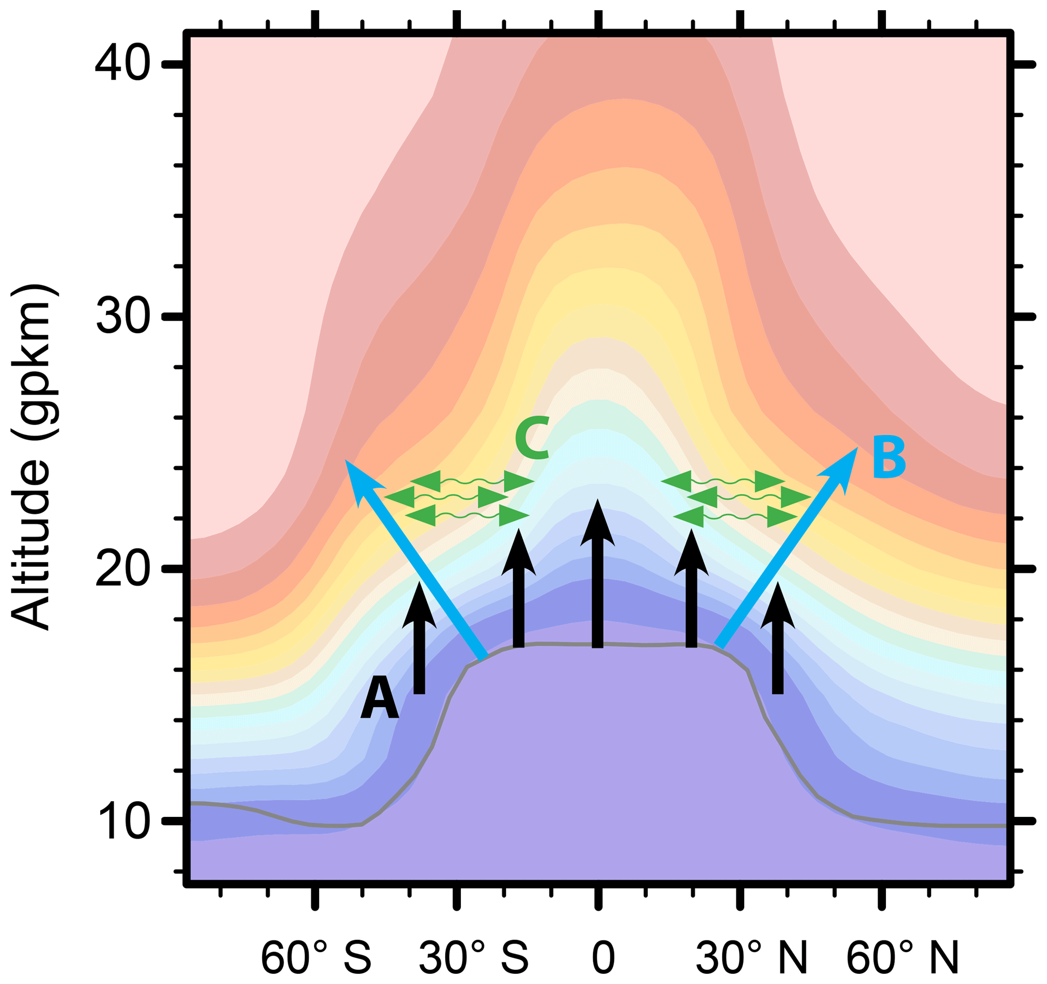
Figure 1Schematic illustration of the location and direction of the effects of the upward shift trend (A), the maximal AoA gradient (B) and the aging-by-mixing decrease (C) on the AoA trend. The colors indicate the climatological zonal mean AoA distribution of the 1960–2000 period in the CMAM REF-C2 simulation.
2.1 Data
Our methodology is motivated by the intention to diagnose the effect of the vertical shift of the circulation due to tropospheric warming and stratospheric cooling (Shepherd and McLandress, 2011; Singh and O'Gorman, 2012; Oberländer-Hayn et al., 2016). For this goal, we have chosen to base our analysis on interpolation to the geopotential height vertical coordinate as an equivalent to the geometric height (for details on the difference between geometric and geopotential height, which is variable with altitude, refer to Andrews et al., 1987). The method of interpolation and vertical shift analysis is described in Sect. 2.2. Among the models that participate in the CCMI-1 project, we were able to apply this methodology to monthly mean data of five chemistry–climate models (CCMs): (1) CMAM; (2) the Goddard Earth Observing System CCM (GEOSCCM, Pawson et al., 2008); (3) the ECHAM/MESSy Atmospheric Chemistry model (EMAC; Jöckel et al., 2016) in two setups with different vertical resolution, L47 (r2i1p1 ensemble member) and L90; (4) HadGEM3-ES (Hardiman et al., 2017); and (5) the NIWA-UKCA (Morgenstern et al., 2009) ensemble of REF-C2 simulations. Basic information on these simulations is summarized in Eichinger et al. (2019; Table 1) and more details on the simulation setups can be found in Morgenstern et al. (2017). The selection of models is based on the availability of the required variables for our analysis and applicability of the method described in Sect. 2.2.
Following Dietmüller et al. (2018), the AoA data require additional modification. For each time step, the AoA value at the tropical tropopause (between 10∘ S and 10∘ N) is subtracted from the AoA values everywhere in the stratosphere (so that AoA =0 at the tropopause). This ensures consistency between the simulations and filters the effect of an increasing path the air has to travel before entering the stratosphere due to the tropopause rise over the period of the study (Held, 1982; Santer et al., 2003; Añel et al., 2006; Shepherd and McLandress, 2011; Oberländer-Hayn et al., 2016; Abalos et al., 2017).
The studied period 1960–2100 has been divided into three parts in agreement with common periods of the REF-C2 model outputs: 1960–2000 (regarded as the reference period in our study; Ref), 2000–2050 (near future; NF) and 2050–2100 (future, F). Those periods correspond well with the ozone depletion and projected recovery (Dhomse et al., 2018; and Fig. S1 in the Supplement for the ozone evolution in the CMAM REF-C2 simulation), which has been highlighted to play a crucial role for driving the BDC trends (Polvani et al., 2017, 2018; Morgenstern et al., 2018). In Sect. 3.2, we analyze the mechanisms of the occurrence of the minimal AoA trends in the extratropical stratosphere and highlight the important role of decreasing RCTT and AbM for the AoA isoline widening. RCTTs are calculated according to the method of Birner and Bönisch (2011) based on residual circulation backward trajectories. AbM is estimated as the difference between AoA and RCTTs (see Garny et al., 2014; Dietmüller et al., 2017, 2018). This means that AbM includes all sorts of resolved and unresolved mixing (see Dietmüller et al., 2017). Due to the methodology of their computation (initialization of backward trajectories), RCTTs and therefore also AbM data are available starting from the year 1970.
For analysis of the causative factors of AbM and RCTT trends in Sect. 3.3, we use CMAM REF-C2 monthly OGWD, non-orographic gravity wave drag (NOGWD), Eliassen–Palm flux divergence (EPFD) and residual mean velocities (, ). These quantities are also interpolated to the geopotential height vertical coordinate by means of collocated monthly geopotential data. We decided not to distinguish between the OGWD and NOGWD in the analysis but take the sum of the two (GWD), partly because we have zonal mean monthly averaged data only and partly because NOGWD parametrization schemes are usually tuned to have only little influence on the LS (Scinocca, 2003).
Throughout the paper, we use information about the tropopause and turnaround latitudes as a measure for BDC widening (Hardiman et al., 2014). The tropopause is computed as a first lapse rate tropopause using the WMO (1957) definition. The turnaround latitudes are computed as the first latitude with a monthly mean vertical residual velocity being lower than or equal to zero going poleward from the Equator on the respective hemisphere and geopotential level.
Trends of all variables have been estimated by the Theil–Sen estimator (Theil, 1950; Sen, 1968), and their significance has been computed using the Mann–Kendall test (Mann, 1945; Kendall, 1975). Where applicable, the statistical significance of differences and correlations has been computed by a Student t test.
2.2 Method
The monthly mean data of all analyzed quantities (in the form Y(time, plvl, lat, long), where Y is a scalar function, time is a time step, plvl is pressure or hybrid level depending on a model, lat is latitude and long stands for longitude) have been linearly interpolated from model levels to the equidistant geopotential height vertical coordinate ( gpkm) using collocated geopotential height values ϕ(time, plvl, lat, long) normalized by the standard gravity at the mean sea level (9.80665 ms−2). The transformation of a vertical coordinate has a direct influence on the value of trends, which can be illustrated by approximating the trend by a local time derivative and by a simple application of the chain rule. Having two scalar functions Y(time, plvl, lat, long) and Y′(time, plvl, lat, long), their local time derivatives in pressure and geopotential coordinates are related as follows:
where ∂ denotes a partial derivative and t is time. In meteorology we generally do not distinguish between Y and Y′. For AoA ( AoA) Eq. (1) yields
Here the local derivative of AoA in the geopotential height vertical coordinate is denoted by subscript ϕ and in pressure coordinates by subscript p.
In Sect. 3.2, we estimate and subtract the effect of the vertical shift of pressure levels on the computation of trends (the second term in Eqs. 1 and 2). Later in the text we call this procedure a correction to the vertical shift of the pressure levels. The correction is based on modification of the geopotential height field (to which we interpolate) so that it does not have a trend (in the long-term sense is zero) and the second term in Eqs. (1) and (2) vanishes. The correction is implemented as follows: where the pressure levels have a significant vertical shift trend, its monthly value (decadal trend divided by the number of months, 120) is cumulatively subtracted from the geopotential field used to interpolate AoA (and other quantities). This is demonstrated in Eq. (3) for the correction in the F period:
ϕc is the geopotential height after correction that corresponds to a pressure level p and meridional position lat in the month i of the F period, t is the pressure level trend (gpm per month) corresponding to p and lat in the given period, and n is the number of months in the respective period (Ref, NF, F). Except for interannual and interseasonal variations, the ϕc vertical coordinate corresponds with the geopotential height of pressure levels at the starting years of the analysis. The resulting trends corrected to the vertical shift of pressure levels are denoted by a superscript c further in the text.
The interpolation to the geopotential height vertical coordinate has been performed for monthly mean data (AoA, RCTT) or for zonal mean monthly mean fields (EPFD, GWD, residual mean velocities). From theory, the interpolation should be made on the finest scale (spatiotemporal) possible. We tried to estimate an upper boundary of the interpolation-connected error by considering an extreme case – we confronted the zonal mean AoA climatology in the 1960–2000 period computed (1) from daily 3-D AoA data interpolated on a daily basis and (2) from climatological zonal mean AoA data interpolated using the 1960–2000 mean zonal mean geopotential data. This is an extreme case, because in our analysis we are interpolating at least monthly mean zonal averages. The difference of resulting AoA climatologies is at maximum around ±0.05 year in the polar regions (not shown). Also in other regions (and in the extratropical stratosphere) the upper estimate of the error connected with interpolation reaches at maximum 1 % of the AoA climatological value. This shows that the application of our methodology to the monthly mean zonal averages will not qualitatively affect our results, especially in the extratropical stratosphere.
2.3 Additional diagnostics
Note that, in the process of changing to a different coordinate system, only values of the original quantities are interpolated. This may be confusing especially in the case of residual mean vertical velocity (), which is usually computed in the models as Pa s−1 as most models use hybrid-pressure coordinates (including CMAM; see Table 3 in Morgenstern et al., 2017) and has to be transformed to meters per second (m s−1) for the standard output. As described in the Supplement of Dietmüller et al. (2018), there are some inconsistencies between the CCMI-1 models regarding this transformation. It was suggested by the CCMI-1 data request to use the log-pressure relationship for this transformation with a scale height of H=6950 m. In our study we interpolate (log pressure, given on pressure levels) to the geopotential height vertical coordinate. Also, the procedure of correction for the vertical shift of pressure levels affects only the distribution of (log pressure) in the modified geopotential coordinate, where we compute the trends, not the units of (log pressure) themselves. Later in the text, we state several times that the correction influences the process of the trend computation only and that it cannot account for the influence of shrinkage on the vertical velocity in log-pressure coordinates (time dependence of the relationship between log pressure and geopotential meter). The validity of the assumption of a constant scale height, which does not take into account the variable vertical shift of pressure levels, is discussed in Sect. 4.2.
In Sect. 3.2 and 3.3 we analyze net tropical upwelling trends and trends of spatially averaged local residual circulation and wave driving. Those quantities in the form of mass fluxes or forces are computed from the original pressure (log-pressure) data interpolated to the geopotential height vertical coordinate. Unlike in pressure, in the geopotential height vertical coordinate system, mass flux (force) has to be computed as a product of velocity (acceleration) and density, which is not a standard output in the CCMI-1 REF-C2 simulations. In our analysis, density is computed using the state equation for dry air. However, the net upwelling mass flux trend is dominated by the density trends (negative trends after the correction for the vertical shift; see Fig. S2 and Table S3 in the Supplement). Therefore we define a kinematic proxy for the mass flux in the form , where overbar denotes the zonal mean and period denotes the average across a period.
The net tropical upwelling kinematical proxy (UP) is then computed by three different methods: (1) direct integration of the mass flux proxy between the turnaround latitudes (UPwstar), (2) evaluation of the residual mean stream function with a vertical integral of the mass flux proxy connected with at the turnaround latitudes between 20 and 40 gpkm (UPvstar), and (3) usage of the quasi-geostrophic version of the DC integral at the turnaround latitudes between 20 and 40 gpkm with a net force in the form (UPDC). See Okamoto et al. (2011) and Abalos et al. (2015) for more information on the different methods for tropical upwelling computation. The meridional and vertical integration was performed using the classical Simpson rule (Süli and Mayers, 2003).
The average density is also used to define the local residual circulation strength (RC) in the form . Neglecting the density trend allows us to focus on the acceleration of the circulation (which is linked with kinematic variables like AoA and RCTT) while still being able to weight the contributions of different vertical levels to the spatial averages from which we compute the trends in Sect. 3.2 and 3.3.
3.1 Extratropical AoA trends in the model simulations
In Fig. 2, the trends of zonal mean AoA for the subset of CCMI-1 simulations are shown for the three periods (Ref, NF and F). The contour lines display the climatological AoA distribution of the respective period. In all periods we see that the analyzed CCMI-1 REF-C2 simulations show the maximum AoA gradient in the region between the tropical LS and the extratropical lower to middle stratosphere (illustrated in Fig. 1).
Here, we focus on the inter-model agreement in projecting the largest negative trend (global or local minimum) in the extratropical lower to middle stratosphere of both hemispheres. The location of those minima does slightly vary between the models but can be found in most cases approximately between 20 and 25 gpkm and 20–50∘ N (ExNH) and 20–50∘ S (ExSH). As long as we do not discuss hemispheric differences, those regions are referred to as Ex regions in the following. Presence of global or local extremes of the AoA changes in the extratropics as well as in other CCMI-1 simulations can be seen in Figs. 1 and 3 in Eichinger et al. (2019).
The best agreement in projecting the minimal trend in the Ex regions is in the NF and F period (Fig. 2). In the NF period, the AoA trends from all analyzed simulations display a well-pronounced, localized Northern Hemisphere (NH) minimum (on the analyzed vertical domain) in the ExNH region. In the NF period, the ExSH AoA trend minima are only local extremes in NIWA and CMAM and have a different structure in GEOS and EMAC-L47. In the F period, there is a pronounced, localized AoA trend minimum in all simulations except EMAC-L47 in the ExNH region and EMAC-L47 and HadGEM in the ExSH region. Particularly in the EMAC-L47 simulation, the trend is strongest in the polar regions below/above 30 gpkm in the NH/SH (Southern Hemisphere). In the Ref period, the models agree only in projecting strong negative AoA trends in the ExSH region. In the NH, the trends are small or more widespread in a broader region with the minimum at the pole.
A localized minimum of the AoA trend in the ExSH region for the 1965–2000 period and in both Ex regions for the 2000–2080 period is visible also in Fig. 3 in Polvani et al. (2018) for their “All-forcings” simulation. In their study, Polvani et al. (2018) apply the Whole Atmosphere Community Climate Model (Marsh et al., 2013; Solomon et al., 2015; Garcia et al., 2017), which is forced as per the CCMI-1 specifications of scenario REF-C2. The localized and almost symmetric AoA trend features in the Ex regions (best pronounced in our analysis in CMAM, HadGEM and NIWA) are collocated with the maximum climatological AoA gradient. This suggests that the trend minima are a geometric consequence of the climatological AoA distribution and its future changes that are aligned with the direction of the gradient. We investigate this in the next subsection and propose possible causes for the changes in the AoA distribution.
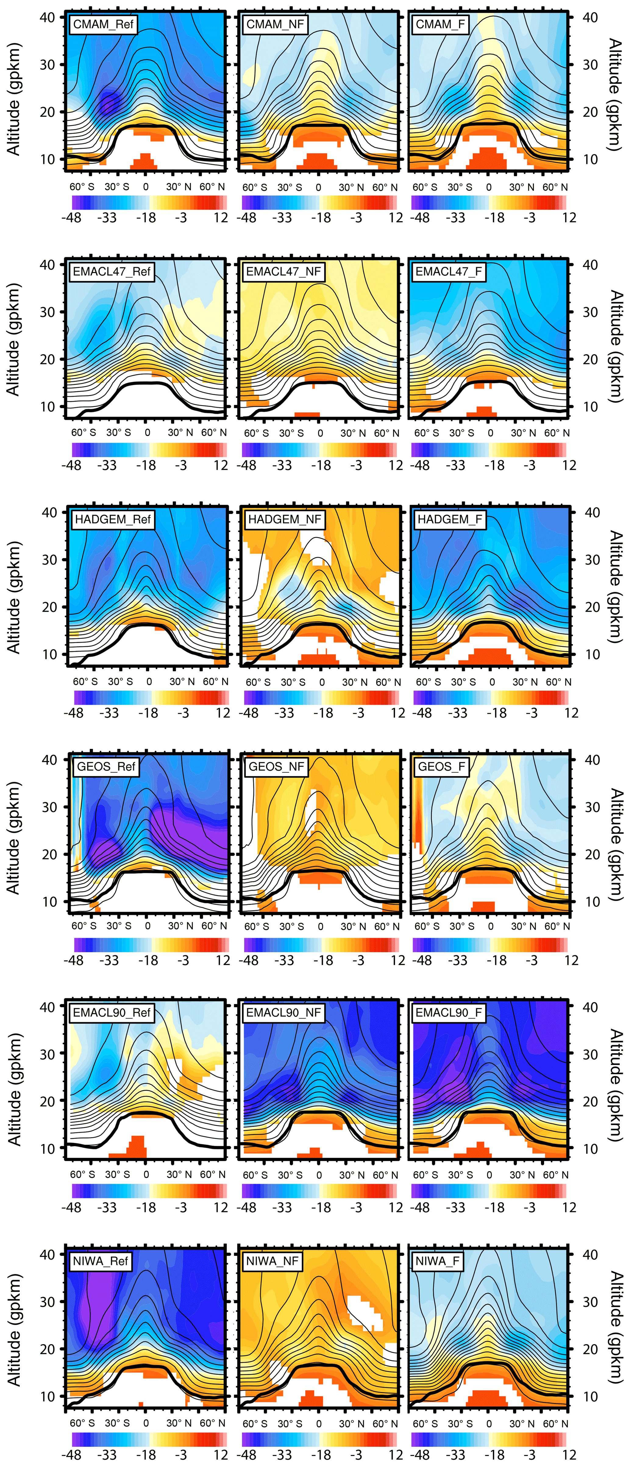
Figure 2Zonal mean AoA trends (days per decade) (colors) and AoA climatology (contours) of the analyzed CCMI-1 REF-C2 simulations. The left column shows the Ref period, the middle column the NF period and the right column the F period. The vertical axis is in geopotential kilometers (gpkm). The mean tropopause position is indicated by the bold black line. White regions mark where the significance level of the trends does not exceed 95 %.
The time evolution of the AoA trends is in agreement with the effect of the phasing out of the ozone-depleting substances, which will lead to a reduction of the BDC trends in future decades (Polvani et al., 2017, 2018; Morgenstern et al., 2018). In Fig. 2, except for the EMAC-L90 REF-C2 simulation, all analyzed simulations are in agreement with this (note that the color bar is different between the periods). The strongest negative AoA trends (globally as well as in the Ex regions) can be detected in the Ref period, and thereafter in the NF period the trend declines. In the F period (mature state of ozone recovery; see Fig. S1), the AoA trends are approaching the magnitudes of the Ref period. In the EMAC-L90 REF-C2 simulation the AoA trend shows the smallest magnitude in the Ref period and an increase in the NF and F periods. For a detailed inter-model comparison of the AoA changes, refer to Eichinger et al. (2019).
3.2 Reasons for the minimal AoA trend in the extratropical stratosphere
In the first part of this section we analyze the vertical shift of pressure levels and connect it with the net upward shift of the circulation (Shepherd and McLandress, 2011; Singh and O'Gorman, 2012; Oberländer-Hayn et al., 2016). In the second part we estimate the effect of the correction for the vertical shift of the pressure levels on AoA, AbM, and RCTT trends and analyze the processes leading to the minimal AoA trend in the Ex regions. This part of the analysis is based solely on the CMAM simulation. However, the findings of Eichinger et al. (2019) show that the AoA distribution and its change are governed by similar processes among the different CCMI-1 REF-C2 models. This suggests that our results can be considered robust also for other CCMI-1 simulations.
3.2.1 Vertical shift and stratospheric shrinkage
Observations and models have shown that the tropopause shifts upward (Santer et al., 2003; Añel et al., 2006) together with the whole tropospheric circulation pattern (Singh and O'Gorman, 2012) due to the tropospheric warming and stratospheric cooling in the course of climate change. The tropospheric warming also influences BDC wave driving by causing an upward displacement of the critical layers for wave breaking (Shepherd and McLandress, 2011). The effect of the upward shift of the circulation on the BDC trends has been highlighted recently by Oberländer-Hayn et al. (2016), where the shift has been divided between the shift of pressure levels and relative to pressure levels. Our methodology (see Sect. 2.2) is developed to diagnose (and subtract) the vertical shift of pressure levels, which is diagnosed as a trend of geopotential height of pressure levels (Fig. 3).
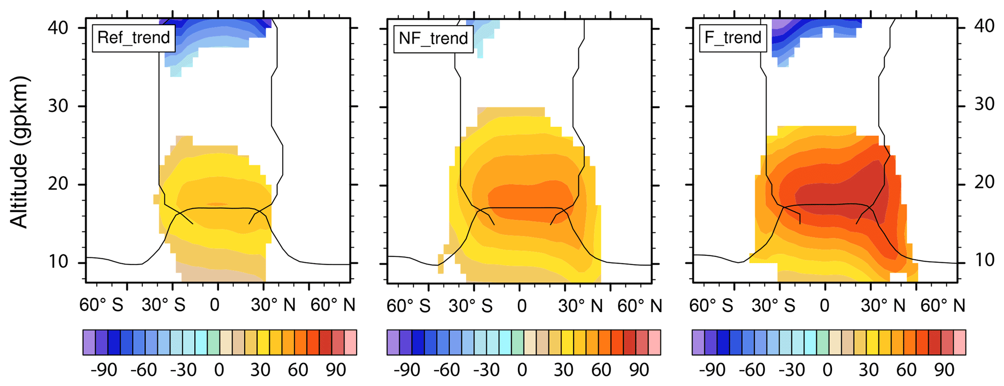
Figure 3CMAM trend of geopotential height of pressure levels (gpm per decade) interpolated to the climatological geopotential height of the selected pressure levels in each period. The mean tropopause and turnaround latitude positions are marked with black lines. Only the trends in the regions where they exceed the statistical significance of 95 % confidence level are plotted.
In Fig. 3 we see that the tropopause is collocated with the region of the largest upward trend of pressure levels in all periods. The trend of the pressure levels in the vicinity of the tropopause in the tropics is around 40, 60 and 80 gpm per decade in the Ref, NF and F period, respectively. Above the tropopause, the trend decreases with altitude and it is not significant higher up. Starting in the middle stratosphere (above around 38 gpkm), the trend is negative. This vertical structure of the pressure level geopotential height trend characterizes the stratospheric shrinkage.
The vertical shift is not globally homogenous; it shows a maximum between approximately 30∘ S and 30∘ N in the Ref period, and it is not significant in the polar regions. In the NF and F period, the area of significance of the trend widens, moving upwards and shifting slightly to the NH. The magnitude of the upward shift trend is smallest in the Ref period and largest in the F period. Interestingly, there is a strong (around 200 gpm per decade) almost significant (at an 85 % confidence level and so not shown) negative trend of the pressure levels in the Ref period in the SH polar stratosphere between 10 and 25 gpkm connected most likely with radiative effects due to ozone depletion and dynamical response of the SH polar vortex.
As described in Eq. (2), the height changes in the pressure levels result in a dependence of the AoA trend on the vertical coordinate system. Since the partial derivative of AoA with respect to the geopotential height is generally positive in the stratosphere (see Fig. 2), the sign of the second term in Eq. (2) is determined by the local derivative of the geopotential height of pressure levels (in our approximation by the trend of geopotential height of pressure levels). Hence, the AoA trend in the geopotential height vertical coordinate is smaller/larger than in pressure coordinates, where the pressure levels rise/sink. In the LS, the pressure levels rise and so the AoA trend is smaller (more negative) in geopotential height than in pressure coordinates. This can be easily illustrated by assuming a situation where the AoA trend in pressure coordinates is zero. But as the pressure levels rise, the fixed geopotential corresponds to increasing pressures over time. These are connected with smaller AoA, which yields a negative AoA trend in geopotential coordinates.
The second part of the vertical shift of the circulation, the vertical shift relative to the pressure levels, is diagnosed in the literature mainly with relation to the tropopause rise. For example, Abalos et al. (2017) assessed the shift by accounting for the tropopause rise by means of remapping to tropopause relative coordinates. The tropopause rise in the geopotential height vertical coordinate and relative to the surrounding pressure levels is shown in Fig. 4.

Figure 4Time evolution of CMAM zonal mean geopotential height (gpkm) of selected pressure levels and of a first lapse rate tropopause averaged between 30∘ S and 30∘ N smoothed by a decadal running average.
The tropopause trend in the geopotential height vertical coordinate can be used in our methodology (Sect. 2.2, Eq. 3) instead of the trend of geopotential height of pressure levels to diagnose the trends also in the tropopause relative coordinate. However, due to neglecting the variable vertical shift of pressure levels (see Fig. 3; stratospheric shrinkage, Lübken et al., 2009), the assumption of a uniform shift equal to the tropopause rise everywhere in the stratosphere may lead to an increasing overestimation of the upward shift effect with distance from the tropopause.
In the next section, we estimate the effect of the vertical shift of pressure levels on the computation of trends. Additional impact of the vertical shift relative to the pressure levels (included in the tropopause rise) on the trend computation is quantified for the trend of the net upwelling only, as the upwelling will undoubtedly reflect the tropopause rise (Oberländer-Hayn et al., 2016), but this is not as certain for the regions higher in the stratosphere.
3.2.2 The effect of the upward shift and AoA isoline widening
In Fig. 5 we show the AoA, AbM, RCTT trends in the Ref, NF and F period computed from spatial averages over the Ex regions (between 20 and 25 gpkm and 20–50∘ N/S) in the standard geopotential height coordinates and after the correction for the vertical shift of the pressure levels (denoted by the superscript c). The bars in Fig. 5 show the trends of the net upwelling proxy computed directly by integration of the mass flux proxy between the turnaround latitudes (UPwstar; see Sect. 2.3) at 20 gpkm before (blue) and after (red) the correction to the vertical shift of pressure levels and also after the correction to the tropopause shift (green). The vertical level of 20 gpkm has been chosen, because it corresponds with the lower boundary of the Ex regions. In Fig. 5 we have chosen to lower the significance threshold to the 90 % confidence level, because many trends are significant between the 90 % and 95 % levels. The information from Fig. 5 is summarized in Tables S1 and S2 in the Supplement, where also values of trends significant at least at the 80 % confidence level are given.

Figure 5Trends of AoA (squares), AbM (crosses) and RCTTs (pluses) averaged over the Ex regions (ExNH on the left, ExSH in the middle) in the Ref, NF and F period in days per decade. Blue markers denote the trends in the geopotential height vertical coordinates and red markers the trends computed after the correction for the vertical shift of pressure levels. On the right (tropics), bars represent UPwstar trends at 20 gpkm before (blue) and after the correction (red) for the vertical shift of pressure levels and also after the correction for the tropopause shift (green) given in 107 kg s−1 per decade. The Ref period is not included as there are no significant UPwstar trends. Presented are only trend values significant at least at the 90 % confidence level. AbM and RCTT trends are computed in a reduced Ref period (1970–2000).
In Fig. 5, both before and after the correction for the pressure level shift, we can see the strongest negative AoA and AbM trends in both Ex regions in the Ref period. The AoA and AbM trends both have the same time evolution, decrease (in absolute values) from Ref to NF and increase again in the F period. On the contrary, both before and after the correction, the RCTT trends are not significant in the Ref period (significant at the 80 % confidence level before the correction in ExNH – see Table S1). In the NF period, the RCTT trends are slightly larger than in the F period both before and after the correction. The AoA trends in the Ex regions are dominated by RCTT trends in the NF period. The time evolution of AoA, AbM and RCTT trends is unchanged after the correction for the pressure level shift.
The difference between the directly computed trend value and the trend value after the correction gives us an estimate of the influence of the pressure level shift on the trend computation. The influence is determined by the second term on the right side of Eqs. (1) or (2), which consists of the vertical gradient of the given quantity and the rate of the pressure level shift that is identical for all quantities but differs between periods. We see in Fig. 5 that for the AoA and AbM trends, the influence grows in future periods in accordance with the time evolution of the trend of geopotential height of pressure levels (Fig. 3). Absolute values of the AoA trend are reduced by 2, 6 and 8 d per decade (i.e., by 6 %, 35 % and 26 %) after the correction in ExNH and by 3, 4 and 5 d per decade (7 %, 27 % and 15 %) in the ExSH for the Ref, NF and F period respectively. The AbM trend is reduced by maximally only 5 d per decade through the correction; however, the 3 d per decade reduction in the ExNH region in NF already accounts for 50 % of the uncorrected trend. In the ExSH region in NF the AbMc trend is no longer significant. RCTT trends are also reduced in absolute value by 2 and 3 d per decade (18 % and 30 %) in the NF and F period in ExNH and by 2 d per decade in both future periods (18 % in NF and 22 % in F) in the ExSH region.
In the Ref period, the UPwstar trends in geopotential height coordinates (blue bars in Fig. 5) are not significant (only at the 80 % confidence level as shown in Table S2). After the correction to the pressure level shift (red bars), the UPwstar trends are reduced by 22 % and 25 % in the NF and F period respectively. In NF and F, both before and after the correction, the UPwstar trend is larger in the F period than in the NF period (as is the case also for AoA and AbM trends).
It has been noted by Randel et al. (2008), Butchart et al. (2010) and Butchart (2014) that the residual circulation changes mainly depend on strengthening of the tropical upwelling. We find a good correspondence with the RCTT and RCTTc trends only for the UPwstar trends corrected for the tropopause shift (Fig. 5, green bars). The correction for the tropopause rise is implemented in a similar manner as for the pressure level shift (Eq. 3); only the tropopause trend instead of the variable pressure level trend is cumulatively subtracted. The UP trend is larger in the NF period than the F period, agreeing with the time evolution of RCTT trends in the Ex regions. The UP trend is larger than the UP trend in NF because, only in the NF period, the tropopause rises less rapidly than the surrounding pressure levels in the CMAM simulation (see Fig. 4). These CMAM results agree well with the results of Oberländer-Hayn et al. (2016), who showed that there is no increase in upwelling when accounting for the tropopause rise. We also did not find any net tropical upwelling trends (differs from UP by containing the time evolving density) after the correction to the pressure level shift and found only one positive trend in the NF period after the correction for the tropopause shift (see Table S3 in the Supplement). In summary, we cannot unambiguously link the time evolution of AoA, AbM and RCTT trends in the Ex regions with the tropical upwelling trends.
We have also analyzed trends of spatial averages of RC in the Ex regions. RC (i.e., the residual circulation strength) is a local measure of acceleration of the residual circulation defined in Sect. 2.3. However, the RC trends are only sparsely significant at the 80 % confidence level and severely reduced in magnitude (see Table 1 in the next section or Table S1 in the Supplement) after the correction for the vertical shift of pressure levels. The possible link between the time evolution of AoA, AbM, and RCTT trends and the acceleration of the residual circulation together with a possible role of wave driving is analyzed also on a seasonal basis in Sect. 3.3.
With the methodology for correction to the vertical shift of pressure levels (Eq. 3), we can now demonstrate the effect of vertical shift on the occurrence of minimal AoA trends in the Ex regions. The distribution of AoAc trends is shown in Fig. 6. Without the effect of vertical shift of pressure levels (upward shift up to about 30 gpkm; Fig. 3), the AoA trends do not form the pronounced, localized, almost symmetric minima in the Ex regions as in Fig. 2 (upper plots for CMAM). Only the global minimum in the Ref period remains in the ExSH region. This is likely due to the impact of ozone depletion in the SH in the Ref period and the methodological limitation that we do not account for the pressure level shift in the SH midlatitudes and polar region due to the lower significance of the vertical shift trend than our threshold (95 % confidence level, Fig. 3).
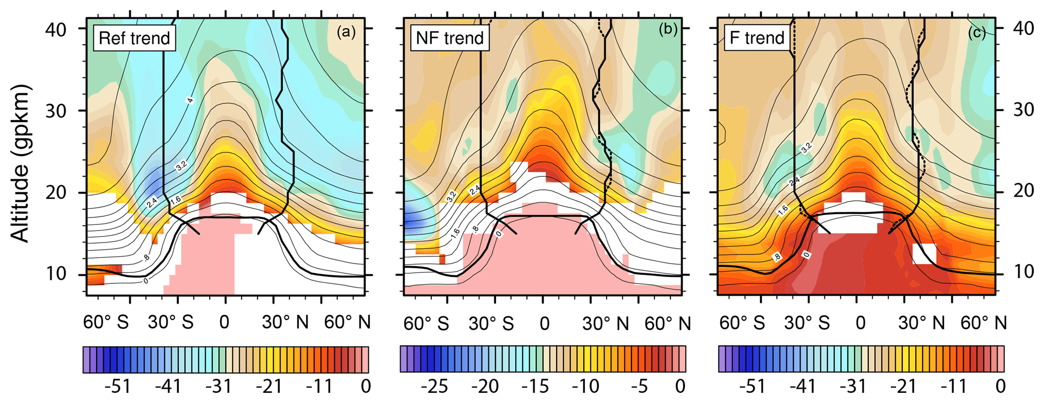
Figure 6CMAM zonal mean AoA annual trend (days per decade) after the correction of the pressure levels trend for the Ref (a), NF (b) and F (c) period, in colors. Only trends that exceed the 95 % significance level are plotted. The mean AoA climatology of the respective period is contoured, and the tropopause and the turnaround latitudes (computed from the residual circulation field interpolated to the geopotential height corrected to the upward shift of the pressure levels) are shown by bold black lines. The turnaround latitude of the preceding period is illustrated by a dashed line.
Figure 6 also shows the mean turnaround latitude positions. The mean turnaround latitude positions between the periods show only small differences in their meridional location. In the NH, there are some visible changes towards a narrowing of the upwelling region below about 26 gpkm and towards a widening above. This is in agreement with the results of Hardimann et al. (2014), who found that the tropical upwelling region narrows below about 20 hPa and widens above. This pattern also appears for turnaround latitude position changes in seasons (not shown), when changes in the SH are pronounced as well.
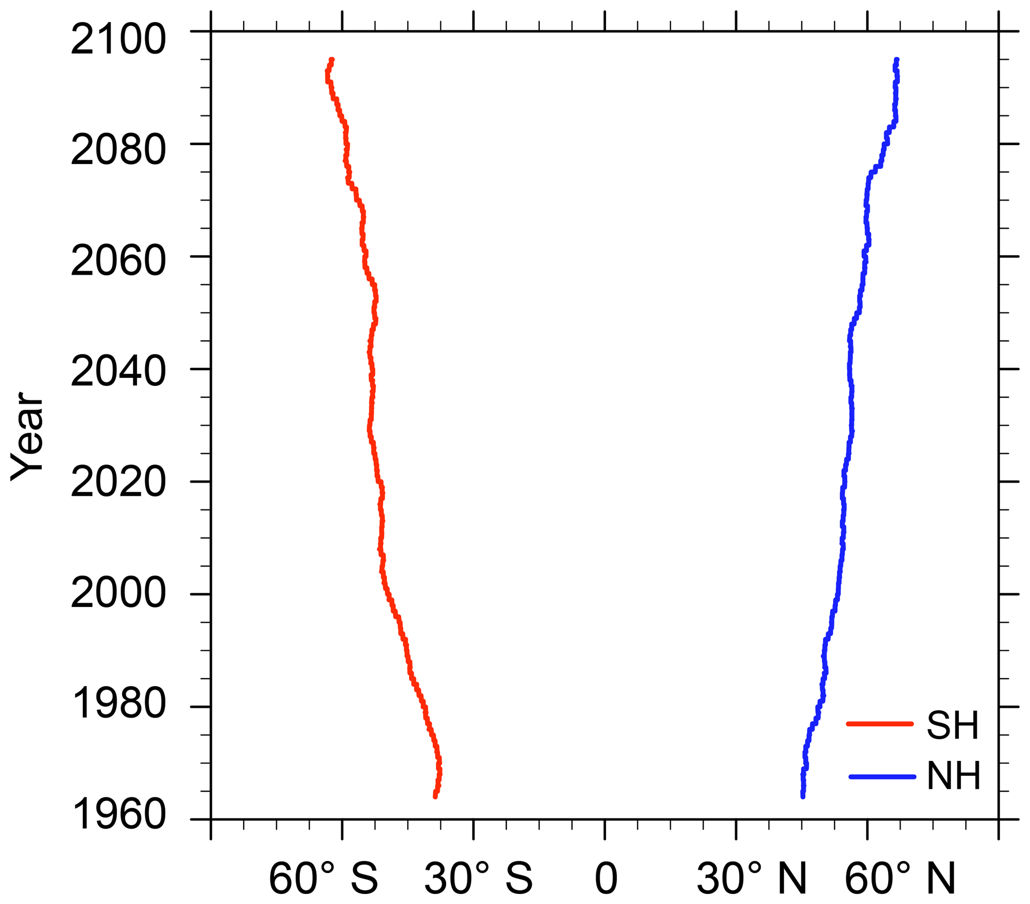
Figure 7Time evolution of the meridional position of the zonal mean AoA =2 years isoline at 20 gpkm after the correction to the upward shift of pressure levels for CMAM. The evolution is smoothed by a decadal running mean.
Figure 7 shows that the AoA distribution in the Ex regions also widens after subtraction of the vertical shift of pressure levels. This widening is related only to AoA isolines and is completely independent of any circulation widening. In Fig. 7 we show the time evolution of a meridional position of intersection of the AoA =2 years isoline with a lower boundary of the Ex regions (20 gpkm) after the correction to the vertical shift. The AoA =2 years isoline crosses the Ex regions initially on their equatorward flanks, and the intersection with 20 gpkm moves poleward of 40∘ S and 40∘ N by the end of the period.
The widening of AoA isolines is partly a direct consequence of the AoA distribution and the negative AoAc trend. Moreover, in the Ex regions, there is a specific role of the decreasing AbM (Fig. 5) for the AoA isoline widening. The climatological distributions of RCTTs (left panel) and AbM (right panel) in the period 1970–2000 overlaid by the AoA climatological distribution (contours) are shown in Fig. 8. Note that the RCTT distribution up to around 30 gpkm between the turnaround latitudes is much broader than the AoA distribution, which has a sharper horizontal gradient than the RCTT distribution. The difference between AoA and RCTTs is largest in the Ex regions and slightly above (up to about 28 gpkm; climatological maxima of AbM in Fig. 8). Due to the negative trend in AbMc in the Ex regions (Fig. 5; see Eichinger et al., 2019, for the zonal mean distribution of the AbM change), the AoA distribution additionally widens as it becomes more similar to the RCTT distribution. Besides the negative AoAc trend and decreasing effect of AbM, the vertical shift relative to pressure levels (tropopause shift) can also be contributing to the widening shown in Fig. 7 in the sense of shifting the climatological AoA isolines upward. The basic features of the CMAM climatologies in Fig. 8 are similar to the RCTT and AbM climatologies from the CCMI-1 REF-C1 simulations (see Figs. 1 and 2 in Dietmüller et al., 2018).

Figure 8(a) CMAM zonal mean RCTTs (year) and (b) AbM averaged over the 1970–2000 period. The thick black lines show the mean tropopause and the turnaround latitude positions in the Ref period.
3.3 Acceleration of the residual circulation and wave driving
The Ex regions lie in the upper flank of the shallow BDC branch. There, AoA has been found to be controlled by both horizontal and vertical residual circulation tendencies and the horizontal mixing tendency (Ploeger et al., 2015b; see their Fig. B1). From Fig. 5 we know that the AoA trends in the Ex regions are dominated by the AbM trends in the Ref and F and by the RCTT trends in the NF period. Note that AbM is not a local quantity. Ploeger et al. (2015b; Lagrangian model study) found that AbM corresponds well with the local mixing integrated along the air parcel pathway. Garny et al. (2014) and Ploeger et al. (2015a) found that the AbM trends in the lowest part of the stratosphere are affected predominantly by changes in the local mixing intensity, but those further above are strongly coupled to the residual mean circulation. This complicates the analysis of possible AbM drivers in the Ex regions, because the Ex regions are located in the transition region between these two regimes. RCTTs are an integrated quantity with climatological values around 1 year in the Ex regions (Fig. 8), and hence they can be influenced by changes in seasonal UP and RC strength (this holds for AbM as well). To gain a better insight into these connections, we study how the RC, UP, local wave drag and vertically integrated drag trends correlate with each other and with the time evolution of AbM and RCTT trends in the Ex regions. The analysis on a seasonal basis is shown in the Appendix.
The Ex regions are located in a region characterized by domination of the meridional residual mean velocity component (see the aspect ratio analysis of Birner and Bönisch, 2011). There is a local direct relationship between and the collocated zonal mean force per unit mass derivable from the transformed Eulerian mean equations (Andrews et al., 1987) under the quasi-geostrophic scaling:
where φ is the latitude and f the Coriolis parameter. Equation (4) provides a direct link between the strength of residual circulation in the extratropical stratosphere and the distribution of the zonal mean zonal force. Besides the trends of the spatially averaged local zonal mean zonal force, we compute also upwelling trends by evaluating the quasi-geostrophic version of the DC integral (Haynes et al., 1991) at the turnaround latitudes (UPDC; see Sect. 2.3). UPDC provides information on wave driving in the whole vertical domain of our analysis. The total drag is in our case composed of the resolved wave driving characterized by EPFD and OGWD and NOGWD from parameterizations. In the Ex regions NOGWD is an order of magnitude smaller than OGWD. Thus, OGWD largely controls the net GWD that is analyzed further. As explained before in Sect. 2.3, in the definition of forces we also replace zonal mean density by zonal mean density averaged over a period to filter out the effect of negative density trends.
In Table 1 we provide annual trends of the spatial averages of total drag (TD), RC, EPFD and GWD scaled by the climatological zonal mean density and corrected for the vertical shift of pressure levels (c). Seasonal trends are shown in Table A1 in the Appendix. In Table 1 we also provide values of trends significant between the 75 % and 90 % confidence level, which are denoted with a superscript +. As explained in detail in the Appendix, EPFD trends are computed from spatial averages between 18 and 25 gpkm and 15–30∘ N/S, and GWD is averaged in the poleward part of the Ex regions between 18 and 25 gpkm and 30–45∘ N/S near its climatological minimum. The values of trends including the density are shown in Table S5 in the Supplement.
Table 1Upward-shift-corrected trend values (c) of total drag (TD, EPFD + GWD) and its components EPFD and GWD multiplied by (all in 10−5 kg m−2 s−2 per decade) and RC (10−3 kg m−2 s−1 per decade) averaged over the Ex regions in the Ref, NF and F period. Presented are trend values significant at least at the 90 % confidence level or at least at the 75 % confidence level (denoted by superscript +); otherwise, the cell is left blank.
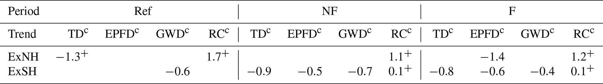
Table 1 shows that in the ExNH neither TDc nor its components over the smaller regions have significant trends in the future periods. In Ref, TDc shows a trend on a weaker significance level. RCc has a positive trend on the weaker significance level in all periods. In the ExSH, GWDc has a significant annual trend in all periods and EPFDc and TDc in the NF and F period. This is reflected in NF and F by the RCc trend at a weaker significance level (+). There is no evidence of a direct link between the RCTT and AbM trends in the Ex regions (Fig. 5) and the trends of the local quantities in Table 1. Keep in mind that, after the correction for the vertical shift of pressure levels, the RCTTc trends are stronger in NF than in F in both Ex regions. AbMc trends are weak or not significant in NF and dominate the AoA trend in the F period. In Table 1 we cannot see any clear time evolution of the magnitude of the trends.
As shown in the Appendix (Table A1), seasonally, RCc and TDc and their components have significant trends in both Ex regions. But again, the time evolution of trend magnitudes does not offer any clear link to the RCTTc or AbMc trends. The evolution of trend magnitudes between the periods differs depending on season and also on the hemisphere. The validity of the quasi-geostrophic local relationship (Eq. 4) is expected to be smaller seasonally (in the equinoctial seasons; Sato and Hirano, 2019), but the link with RCc is especially weak for GWDc regarding seasonal correlations (Table S4) or seasonal (Table A1) and annual trends (Table 1).
To conclude, after the subtraction of the vertical shift of pressure levels, the AbMc and RCTTc trends in the Ex regions cannot be easily linked to the upwelling or local residual circulation changes. The link to the wave-driving trends in the NF and F period is even less clear. This indicates that additional mechanisms may be involved, for example the effect of stratospheric shrinkage could explain some of the AoA changes. Moreover, our diagnostic methods, in particular regarding the sparse spatiotemporal sampling of GWD effects, may not meet the needs for accurate analysis of the connections between the processes.
4.1 Speeding up of the BDC and wave driving
In several studies a physical connection between changes in AoA, AbM and RCTTs; the speeding up of the residual mean circulation (see Birner and Bönisch, 2011; Li et al., 2012; Garny et al., 2014; Ploeger et al., 2015a); and increasing wave driving by changes in the resolved and unresolved extratropical wave forcing (e.g., Okamoto et al., 2011; Shepherd and McLandress, 2011; Butchart, 2014) has been postulated. In the present study, after the correction to the vertical shift of pressure levels, we could not find a simple link between trends of wave driving (TDc, GWDc, EPFDc and UP); net upwelling (UP and UP, Fig. 5 and Table A2); local residual circulation strength (RCc) in the extratropical lower to middle stratosphere (Tables 1 and A1); and trends of AoAc, AbMc and RCTTc (Fig. 5), i.e., quantities representing transport connected with the BDC. The fact that our results do not fully support the hypothesis indicates that additional mechanisms may be influencing transport and dynamics in the studied regions (as discussed in Sect. 4.2), but it also partly stems from peculiarities of our analysis. Namely, our analysis is focused on the Ex regions, which do not belong fully to the altitudinal range of the shallow BDC branch and lie, e.g., on the interface between the two dynamical regimes influencing the AbM (Garny et al., 2014; Ploeger et al., 2015a). Also, our approach of dividing the REF-C2 simulations into three periods is different from the above-mentioned studies and brings along the novel opportunity to analyze the time evolution of trends of different quantities at the expense of more difficult acquisition of significance.
The trends computed in the geopotential height vertical coordinate after the correction for the pressure level shift (c) should be comparable to the trends in pressure levels (Eqs. 1 and 2). Hence, it is precisely due to the methodology (choice of significance levels, periods, seasons, trends vs. differences) that we did not find as robust changes in wave drag in connection with the acceleration of the residual mean circulation as reported in other studies based on pressure coordinates (e.g., Okamoto et al., 2011; McLandress and Shepherd, 2009; Shepherd and McLandress, 2011). However, this does not hold for analyses based on log-pressure coordinates, as they include the effect of the vertical shift of pressure levels (see discussion in Sect. 4.2). If the vertical shift of pressure levels is not subtracted, the emerging link between the trends or changes in general may be simply induced by the common impact of the vertical shift and not by the structural changes.
We would like to point out one particular result of our wave-driving analysis – a weak correspondence between GWDc and the RCc trends. Although the quasi-geostrophic theory itself does not support GWs, it is often used to study GW effects on the circulation. As shown in the Appendix (Fig. A1), the correlation between and GWD is weaker than for EPFD, suggesting that the quasi-geostrophic local relationship (Eq. 4) is less valid for GWD. Also the weak correspondence between GWD and RC trends argues against a direct relationship (of absolute values) as in Eq. (4). We do not argue that the lower validity of the local relationship (Eq. 4) for GWD implies that the quasi-geostrophic approximation is generally unfit for studies of the GWD effects. We argue that the complex role of GWD on transport in the stratosphere cannot be judged from the zonal mean monthly mean data output only, as the average value is not fully representative of the GWD distribution.
GWs are intermittent (e.g., Hertzog et al., 2012; Wright et al., 2013) and asymmetrically distributed (Hoffmann et al., 2013, 2016; Šácha et al., 2015; Pišoft et al., 2018) in nature. This intermittency and asymmetry of the spatial distribution of GWD (OGWD in particular) is to some extent present also in the CCMI-1 simulations. For example, a crucial role of the zonally asymmetric OGWD distribution for its interannual variability has been shown by Šácha et al. (2018) for a CMAM specified dynamics simulation (McLandress et al., 2013), which uses the same parameterization of orographic GWs as the CMAM REF-C2 simulation analyzed in this study. The zonal mean data can hide different effects on the residual circulation due to the zonally asymmetric distribution of the GWD (Šácha et al., 2016) present in the models, and monthly mean output can mask the extreme GWD values. Note that also the widely used DC principle relies on zonally symmetric forces (Haynes et al., 1991). Clearly, there is a need for provision of as-frequent-as-possible 3-D GWD output (complex, not only the induced zonal acceleration component) in connection with reporting of extreme values during the time window in addition to average values to properly diagnose the possible GW effects present in the models.
4.2 Stratospheric shrinkage
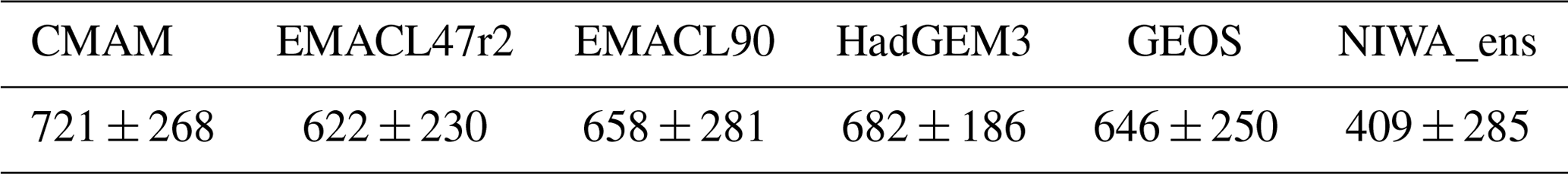
In Sect. 3.2.1 (Fig. 3) we analyzed the vertical shift of pressure levels, which results in a so-called stratospheric shrinkage. Although our methodology accounts for the effect of the vertical shift of pressure levels (stratospheric shrinkage) in the process of trend computation, the effect of decreasing geometrical distances between pressure levels in the course of the model simulation, which can directly influence the AoA, RCTTs and AbM, cannot be quantified in our analysis. To our knowledge, this effect has not been mentioned in relation to the possible causative factors of the AoA trend (or BDC acceleration) before. For example in Table 2 we show how the mean distance between the 1 and 100 hPa levels will change between the 1960s and the 2090s. In the analyzed simulations, the 100 hPa level in the tropics will be closer to the 1 hPa level by about 400–700 m in the 2090s than in the 1960s. Depending on the variable geopotential height of pressure levels and distances between the two levels at the start of the analysis in the simulations, the differences in Table 2 range from 2.33 % for CMAM to 1.3 % for NIWA of the original distance in the 1960s in the tropics. Assuming a constant speed of advection in the vertical, this directly reduces the RCTTs (for vertical velocity of an order of 10−4 ms−1 it takes 84 d less to travel the distance shrunken by 720 m). The effect on AbM or mixing in general can be of a more complex, possibly nonlinear, nature.
Table 2The change in the mean distance (in geopotential meters) between the 1 and 100 hPa levels in the tropics between the 1960s and the 2090s for the analyzed REF-C2 CCMI-1 simulations.
As pointed out before, we also cannot account directly for the shift relative to the pressure levels. Typically in the literature (Oberländer-Hayn et al., 2016; Abalos et al., 2017), the tropopause is taken as a proxy for the upward shift relative to pressure levels. Otherwise, the possibly non-homogeneous shift relative to pressure levels in the stratosphere cannot be objectively assessed. Note also that the shift related to the tropopause can become very complicated to disentangle. The whole region changes its structure because of the increasing occurrence of double and multiple tropopauses due to increasing baroclinicity in the course of climate change (Castanheira et al., 2009; Castanheira and Gimeno, 2011; Wang and Polvani, 2011; Añel et al., 2012).
In Fig. 4 (Sect. 3.2.1) we show how the first lapse rate tropopause in CMAM shifts relative to pressure levels between 30∘ S and 30∘ N for the CMAM REF-C2 simulation. The averaged tropopause shifts by about 1 gpkm in the course of the simulation. Such a shift is in the range of the tropopause trends from the Coupled Model Intercomparison Project (CMIP5) ensemble mean in the tropics (Fig. 7a in Vallis et al., 2015). It corresponds also to the net equatorial tropopause height change from the simulations analyzed by Oberländer-Hayn et al. (2016) and Abalos et al. (2017), who diagnosed a net tropopause shift of 430 m in the global average. In the whole period of the analysis, the tropopause pressure changes by almost 10 hPa. Depending on the vertical shift of the stratopause (assuming that it will follow the pressure levels rather than the tropopause), the tropopause shift causes additional stratospheric shrinkage.
Figure 4 also shows that the rate of the tropopause shift relative to pressure levels almost perfectly follows the division into the periods used in this study. The tropopause rises rapidly relative to pressure levels in the Ref and F period, when we found the biggest AbM and AoA trends (Fig. 5). In the NF period, there is no visible shift of the tropopause relative to pressure levels, which corresponds well with the small (ExNH) or insignificant (ExSH) AbM trends. The rate of the tropopause shift (and possibly of the net stratospheric shrinkage) thus correlates with the time evolution of AbM trends. However, at this stage we cannot provide a detailed or analytical description of the mechanism.
It has been shown before (i) by Shepherd and McLandress (2011) that the EPFD changes associated with GHG increases in the subtropics are largely controlled by the upward displacement of the critical layers for wave breaking and (ii) by McLandress and Shepherd (2009) and Okamoto et al. (2011) that the OGWD changes are linked to the upward shift of the subtropical jet (Son et al., 2009). Also, Eichinger et al. (2019) found that the mixing changes, as well as the inter-model spread, are connected to changes (upward shift) of the background potential vorticity (PV) gradient in the CCMI-1 simulations. All of those studies were based on pressure coordinates and so the shift they are referring to is the shift relative to pressure levels (tropopause shift).
The RCTT trends do not reflect the time evolution of the shift relative to pressure levels directly (i.e., the trend is larger in the NF period than in the F period). The reason can lie in the strong dependence of RCTTs on the tropical upwelling. Tropical upwelling is the only quantity (as explained in Sect. 3.2.1) for which we computed the trends also in coordinates corrected to the tropopause shift (Tables S2, S3 and S6 in the Supplement). After the correction to the tropopause shift, the net tropical upwelling shows the same time evolution of trends as RCTTs. This is caused by a missing vertical shift of the tropopause relative to pressure levels in NF in CMAM. Future research is needed regarding a possible cause and robustness of this feature between the models.
Finally, there are important consequences for trend analyses based on log-pressure coordinates in connection to the stratospheric shrinkage. Unlike in the pressure coordinates, the vertical shift of pressure levels is reinstated in log-pressure coordinates due to the utilization of a constant scale height (H) in the conversion from the pressure coordinates. Therefore the trends computed in log-pressure coordinates are influenced by the effect of the variable vertical shift of pressure levels. Moreover, the choice of constant H also leads to the artificial increase in the log-pressure vertical velocity (see the Supplement of Dietmüller et al., 2018, for details on the transformation) due to neglecting the shrinking geometrical distance between the pressure levels.
In a subset of CCMI-1 REF-C2 simulations, we have pointed out a remarkable pattern of similarity in the morphology of the stratospheric AoA trend, especially in the future periods (2000–2050 and 2050–2100). These are the regions of minimal AoA trends, which are located in both hemispheres between 20 and 25 gpkm and between 20–50∘ N (ExNH) and 20–50∘ S (ExSH). We hypothesized that these minima are connected with the climatological AoA gradient and the previously known AoA trend drivers: (a) upward shift of the circulation (Oberländer-Hayn et al., 2016; Abalos et al., 2017) and (b) decreasing AoA trend consisting of the RCTT (residual circulation transit times) and AbM (aging by mixing) contribution (Garny et al., 2014). Both mechanisms also influence the widening of the AoA isolines in the Ex regions.
From the net upward shift of the circulation, the part connected with the vertical shift of the pressure levels has been diagnosed and the so-far-neglected stratospheric shrinkage pattern has been pointed out. We then showed that the AoA, AbM, RCTT (in the Ex regions) and the net tropical upwelling trends are reduced when accounting for the vertical shift of pressure levels. Moreover, the local residual circulation strength (RC) does not exhibit any trends when accounting for the shift (only at a weaker significance level). After the vertical shift correction, we could not find a direct relationship between the total zonal mean wave drag and its components (resolved and unresolved), the seasonal RC or upwelling trends, and the time evolution of the AbM and RCTT trends. This indicates that additional mechanisms may be involved. For example, we discuss a mechanism of how the stratospheric shrinkage can affect the AoA changes. Moreover, our diagnostic methods, in particular regarding the sparse spatiotemporal sampling of GWD effects, may not meet the needs for accurate analysis of the connections between the processes in the models, for which more detailed GWD output would be needed.
The analysis is based on geopotential height coordinates, but the argument that the upward shift (together with AoA isoline widening) is necessary for the visual pattern of localized AoA trend minima in the extratropical stratosphere holds also in pressure coordinates. The location of the minimal AoA trends is in the best vertical range for the AirCore measuring tool (Engel et al., 2017), and their easy visual detectability makes them the best regions for AoA trend observations. The detection of the localized trend minima in the Ex regions in observations could provide validation of the processes that lead to their formation in the models. Those are the upward shift of the circulation, the AoA decreasing trend and most importantly its aging-by-mixing (AbM) component that can be connected with the fine dynamical features of the model's lower stratosphere. To gain more insight in future climate projections, we particularly suggest inter-model analysis of the stratospheric shrinkage, including the time evolution of the vertical shift of the tropopause and its effect on the stratospheric circulation.
All data CCMI-1 used in this study can be obtained through the British Atmospheric Data Centre (BADC) archive (ftp://ftp.ceda.ac.uk, last access: August 2018). For instructions for access to the archive, see http://blogs.reading.ac.uk/ccmi/badc-data-access, last access: December 2018).
There are indications that changes in the unresolved wave drag are often compensated for by changes in the resolved wave driving (McLandress and McFarlane, 1993; Cohen et al., 2013, 2014). This so-called “compensation mechanism” is present also in comprehensive climate model projections of the BDC change (Sigmond and Shepherd, 2014) and complicates the possibility of clearly separating the effects of individual wave drag components. The compensation needs to be taken into account to identify the areas where the individual drag components can influence the advection to the Ex regions. Therefore, we analyze the wave drag distribution and the occurrence of compensation near the Ex regions.
In Fig. A1a, we show the total drag (GWD+EPFD) climatology (contours) overlaid over the ratio of unresolved to resolved wave drag (GWD ∕ EPFD). Fig. A1b and c show the climatological distribution of EPFD and GWD, respectively. We see that GWD has its climatological minimum slightly below the Ex regions around 18 gpkm and is dominant (bigger than EPFD) in the lower stratosphere only in the NH (Fig. A1a, red color). This extratropical lower stratospheric region is located exactly around the NH turnaround latitude from 16 to 22 gpkm. In the location of the GWD minimum in SH, GWD is smaller than EPFD. Other regions of GWD dominance are scattered higher in the stratosphere.
In the extratropical stratosphere, regions with the same sign of GWD and EPFD prevail (Fig. A1a, red and antique white colors). The ratio is shown for the Ref period and differs only slightly in the NF and F period when corrected to the pressure level shift (not shown). The regions of the lower stratospheric minima of GWD are collocated with the saddle-like regions in the EPFD distribution around 16 to 22 gpkm (Fig. A1b). Those regions are positioned on the upper flank of the subtropical jets of both hemispheres but are more pronounced in NH, where the GWD is stronger. The total drag distribution (contours in Fig. A1a) largely copies the EPFD distribution, but it is smoother in the lower stratosphere as the saddle-like pattern from the EPFD distribution is filled by GWD. This can be considered as a fingerprint of the compensation, and indeed this region includes the 70 hPa level, where Cohen et al. (2013) demonstrated the compensating effects between OGWD, EPFD and NOGWD for driving of the residual circulation.
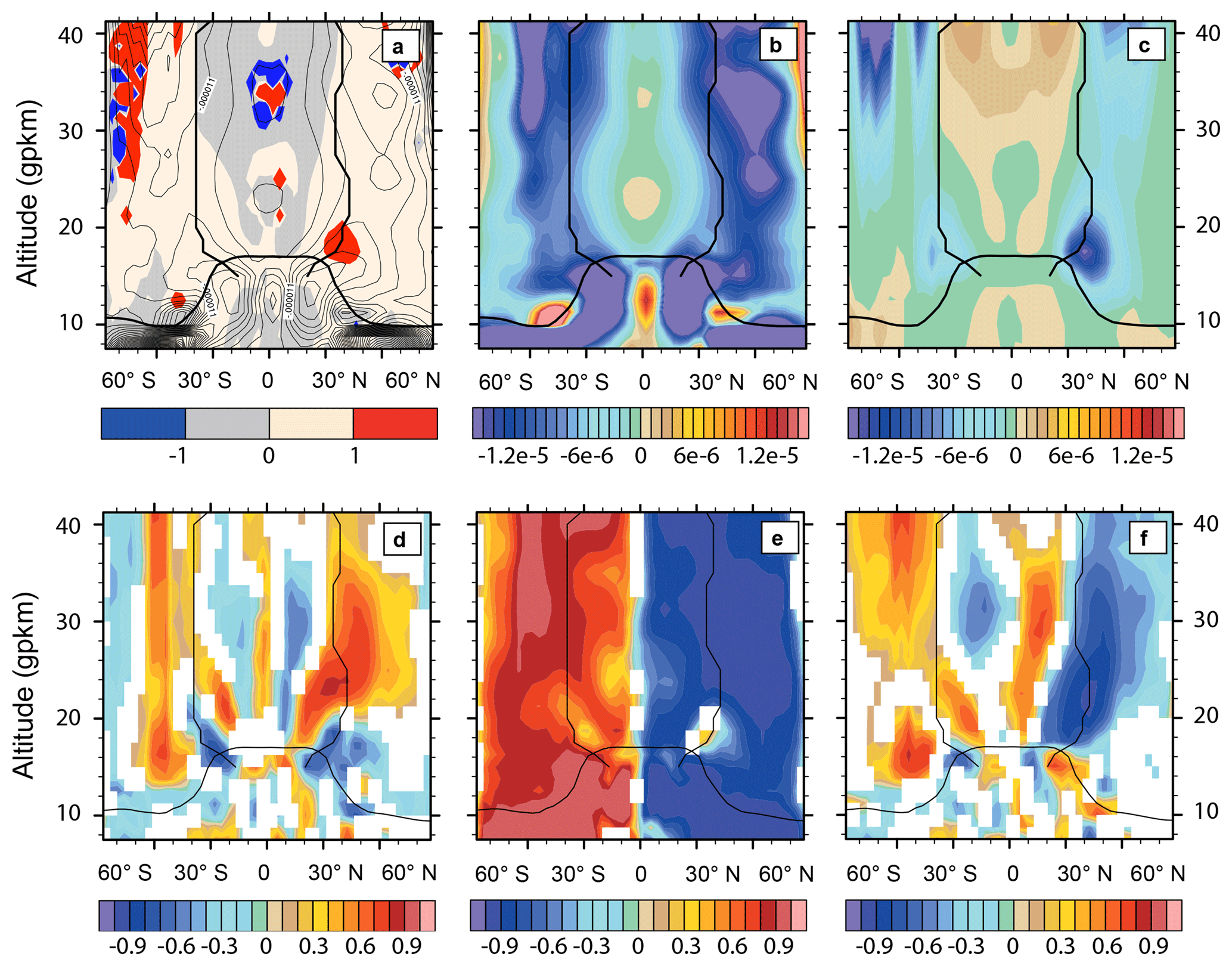
Figure A1(a) GWD ∕ EPFD ratio of the Ref period. The color scale is chosen so that the regions with the absolute value of zonal mean zonal GWD stronger than EPFD are highlighted. The contours show the total drag Ref climatology. (b) EPFD and (c) GWD climatology of the Ref period (units kg m s−2). Correlations between (d) GWD and EPFD, (e) EPFD and , and (f) GWD and in the Ref period. The vertical axis is in geopotential kilometers (gpkm). The plots are overlaid by the mean tropopause and turnaround latitude positions in the Ref period. Only regions with a statistical significance of correlations exceeding the 95 % confidence level are plotted.
Further information on the compensation is provided in Fig. A1d, e, f. Here we show correlations between the drag components and . For brevity, only the annual mean correlations in the Ref period are shown, although the compensation between wave drag components and the relationship with the residual circulation is changing during the year (see Table S4 in the Supplement for the correlations computed after the correction to the vertical shift of pressure levels.
In Fig. A1d, the distribution of negative correlations, which indicate compensation between the drag components, agrees well with the location of regions of minimum (strongest) GWD (EPFD saddle regions). Otherwise, in the extratropical stratosphere we find mainly positive GWD and EPFD correlations. The localization of the compensation is confirmed also by correlations of GWD and EPFD with (Fig. A1e, f). In the extratropical stratosphere, EPFD does not have significant correlation with solely in the region of minimal GWD in the NH (low value of correlation also in the location of the SH GWD minimum). GWD is strongly correlated with in those regions. Elsewhere, the high absolute values of correlation between EPFD and (generally higher than 0.7) show a good validity of the direct relationship between the zonal mean zonal force and (Eq. 4), although neither EPFD nor are computed using a quasi-geostrophic formula. The correlation of GWD with has a more patchy structure and does not reach correlation values as high as for EPFD. In ExNH, GWD is better correlated with than in the ExSH region.
Due to the climatological distribution and occurrence of compensation, we do not average the drag components over the whole Ex regions. Instead, EPFD trends are computed from a spatial average between 18 and 25 gpkm and 15–30∘ N/S, i.e., slightly lower and more equatorward than the location of Ex regions. There, EPFD dominates the driving of the advection to the Ex regions. GWD is averaged in the poleward part of the Ex regions between 18 and 25 gpkm and 30–45∘ N/S near its climatological minimum. For direct comparison with the RC trends, the total drag is averaged over the whole Ex regions. The occurrence of compensation within the averaging domain means that the total drag can have a significant trend, regardless of the significance of the trends of its components. Because the compensation is also present around the turnaround latitudes at 20 gpkm, where we evaluate the DC integral for computation of the mean upwelling (UPDC), we do not separate the individual drag components (UPDC trends are given in Table A2).
As shown in Table A1, seasonally, RCc and TDc and their components have significant trends in both Ex regions. The seasonal trends have the largest magnitude in absolute value in both Ex regions in the Ref period in the DJF and MAM season. In JJA and SON the trends are smaller in absolute value in the ExNH or reverse sign towards weakening of the drag (except GWD) and deceleration of the circulation in the ExSH. In the following, we will focus on seasonal trends in the NF and F periods and on the issue of different evolution of trend (RCTTc vs. AbMc) in the future periods.
First, note that the seasonal TDc, EPFDc and GWDc trends are generally larger in the NF than F period in both Ex regions, which excludes the possibility of a direct link between the AbM trends and local wave drag. For RCc, we can see stronger trends in F than NF in the MAM and SON season in the ExNH region and in the JJA season in the ExSH region. In other seasons the trend is not significant in both future periods or is higher in the NF period. In ExNH, all drag trends are accompanying RCc trends in MAM for both future periods and in JJA only for the NF period. However, the drag trends in MAM do not reflect the almost doubling of the magnitude of the MAM RCc trend between the NF and F period. In the ExSH region, local drag trends accompany the RCc trend in both future periods only in DJF. In this season, the absolute value of trends decreases more strongly for drag than for RCc between NF and F. In the ExSH, the link with RCc is especially poor for the GWDc trends. The reason for this may be that in the ExSH region GWDc is only weakly correlated with (annual mean correlation equal to 0.31; see Table S4).
Table A1Upward-shift-corrected trend values (c) of total drag (TD, EPFD + GWD) and its components EPFD and GWD multiplied by (all in 10−5 kg m−2 s−2 per decade) and RC (10−3 kg m−2 s−1 per decade) averaged over the Ex regions in the Ref, NF and F period. Presented are trend values significant at least at the 90 % confidence level or at least at the 80 % confidence level (denoted by superscript +); otherwise, the cell is left blank.
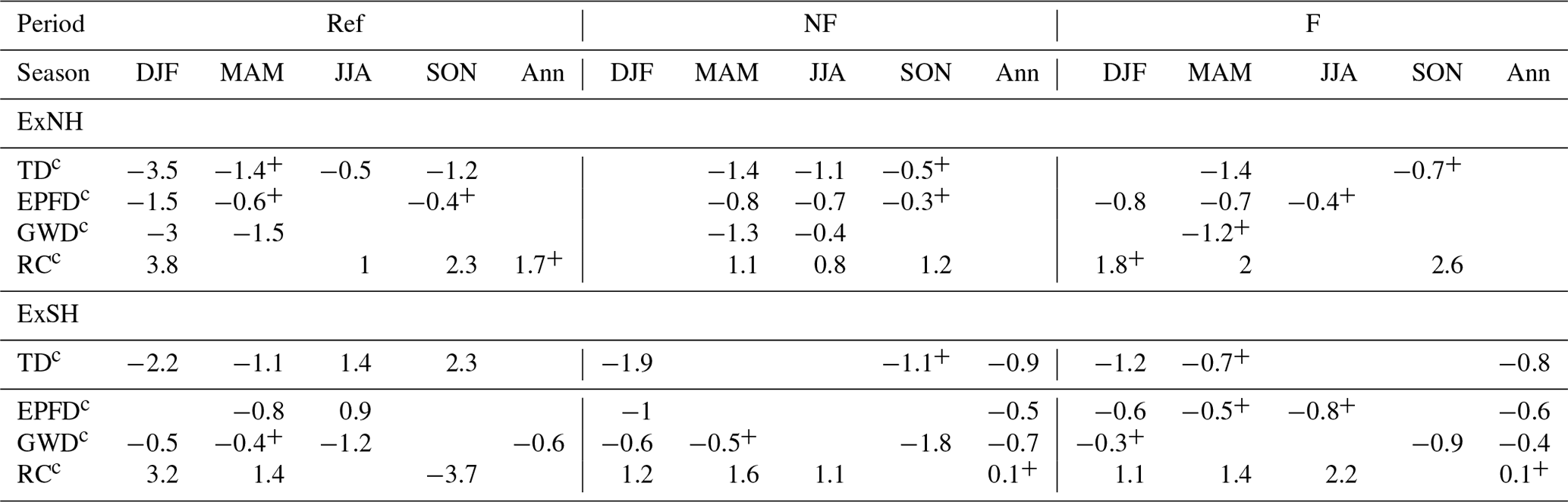
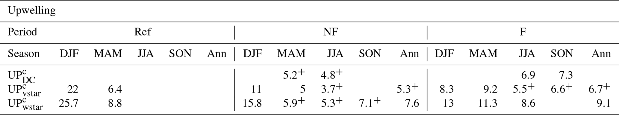
Table A2Trends of UP (in 107 kg s−1 per decade) computed with three different methods after the correction for the vertical shift of pressure levels (UP, UP and UP) in the Ref, NF and F period. Presented are trend values significant at least at the 90 % confidence level or at least at the 80 % confidence level (denoted by superscript +); otherwise, the cell is left blank.
In the ExSH region, when significant, the seasonal RCc trends are only slightly higher in F than in NF. Nevertheless, in ExNH, the seasonal RCc trends are more than twice as large in F than in NF. This correlates better with the AbMc trend evolution in the ExNH. However, in the ExSH region, we cannot link the magnitude of the seasonal RCc trends to the time evolution of the AbMc trend. The AbMc trend in ExSH is not significant in NF and is then larger in F than the ExNH AbMc trend. Seasonal trends of TDc, EPFDc and GWDc show some small increase from the NF period to the F period in ExNH but rather the opposite in the ExSH region. This does not allow a clear link to the time evolution of the RCc or AbMc and RCTTc trends.
In Table A2 we show seasonal UP trends computed with different methodologies after the correction for the vertical shift of pressure levels. The trends of net upwelling (including time evolving density) are given in Table S6 in the Supplement. Trends of another drag-based quantity (UP) show a clear strengthening of the integrated TDc in the F period but are only sparsely significant with different seasonality than the upwelling estimates based on the residual mean circulation, indicating lower validity of the quasi-geostrophic assumption.
From the three methodologies, two based on the residual mean velocities (UP, UP) yield almost identical results regarding seasonal occurrence of the trends. The time evolution of the seasonal UP and UP trends varies between seasons. In the DJF season both trends are largest in Ref and smallest in the F period, but in MAM the trends are largest in F and smallest in the NF period. This is true also for the annual trends and trends in other seasons that are not significant in the Ref period.
The UP inferred from the integral of TDc at the turnaround latitudes have only weakly significant seasonal trends in MAM and JJA in the NF period and significant trends in the JJA and SON season in the F period. The JJA trend is higher in F than NF. We can only speculate that the UP trends in MAM and JJA in the NF period can be connected with the local drag trends in the ExNH (Table 1), but this is almost certainly not possible for the UP JJA and SON trends in the F period. One possible reason is that the seasonal UP trends in the F period are driven by changes in drag above the Ex regions, where TDc has been spatially averaged. The RCc trends correlate well with the seasonal UP and UP trends, with the exception of the strong UP and UP trends in DJF in the NF period accompanied by small (missing in the ExNH) RCc trends in this season and period.
To conclude, the UP and UP trends do not allow a clear link to the time evolution of AbMc or RCTTc trends, as they have a different time evolution in the DJF, MAM and JJA seasons between the periods.
The supplement related to this article is available online at: https://doi.org/10.5194/acp-19-7627-2019-supplement.
PŠ performed all the analyses and wrote the article together with RE. JAA, LdlT, PP and HG made substantial contributions to the conception of the study and interpretation of the results and participated in drafting the article. SD provided the RCTTs data, helped with their analysis and commented on the paper. In their role as CCMI model PIs, the other authors contributed information concerning the analyzed models, commented on the manuscript and helped to revise the paper.
The authors declare that they have no conflict of interest.
This article is part of the special issue “Chemistry–Climate Modelling Initiative (CCMI) (ACP/AMT/ESSD/GMD inter-journal SI)”. It is not associated with a conference.
We acknowledge the modeling groups for making their simulations available for this analysis and the joint WCRP SPARC–IGAC Chemistry–Climate Model Initiative (CCMI) for organizing and coordinating this model data analysis activity. We thank the British Atmospheric Data Centre (BADC) for hosting the CCMI-1 data archive. We acknowledge the UK Met Office for use of the MetUM. The EMAC simulations have been performed at the German Climate Computing Centre (DKRZ) through support from the Bundesministerium für Bildung und Forschung (BMBF). DKRZ and its scientific steering committee are gratefully acknowledged for providing the HPC and data-archiving resources for the consortial project ESCiMo (Earth System Chemistry integrated Modelling). The NIWA program CACV was supported by the NZ Government's Strategic Science Investment Fund (SSIF). The authors wish to acknowledge the contribution of NeSI high- performance computing facilities to the results of this research. New Zealand's national facilities are provided by the New Zealand eScience Infrastructure (NeSI) and funded jointly by NeSI's collaborator institutions and through the Ministry of Business, Innovation & Employment's Research Infrastructure program (https://www.nesi.org.nz, last access: August 2018). The GEOSCCM is supported by the NASA MAP program, and the high-performance computing resources were provided by the NASA Center for Climate Simulation (NCCS). Petr Šácha is supported through a postdoctoral grant of the Xunta de Galicia ED481B 2018/103. Further, Petr Šácha would like to acknowledge Felix Ploeger and Mohamadou Diallo for their comments and suggestions at the beginning stages of the analysis and would like to thank Rachel White, Harald Rieder, Joan Alexander and Kaoru Sato for their comments and discussions about the wave driving and compensation mechanism. Roland Eichinger, Hella Garny and Simone Dietmüller acknowledge funding from the Helmholtz Association under grant VH-NG-1014 (Helmholtz-Hochschul-Nachwuchs-forschergruppe MACClim). Olaf Morgenstern acknowledges funding by the New Zealand Royal Society Marsden Fund (grant 12-NIW-006). Neil Butchart and the development of HadGEM2-ES was supported by the joint DECC–Defra Met Office Hadley Centre Climate Programme (GA01101) and the European Commission's Seventh Framework Programme StratoClim project 226520. Petr Pišoft was supported by GA CR under grant nos. 16-01562J and 18-01625S. Juan A. Añel was partially supported by a Ramón y Cajal Fellowship (RYC-2013-14560).
The authors would like to thank the two anonymous referees and the co-editor Gabriele Stiller for all their help towards improving the manuscript.
This research has been supported by the Government of Spain (grant no. CGL2015-71575-P) and by the Czech Science Foundation (GAČR) under GA CR under grant nos. 16-01562J and 18-01625S.
This paper was edited by Gabriele Stiller and reviewed by two anonymous referees.
Abalos, M., Randel, W. J., Kinnison, D. E., and Garcia, R. R.: Using the Artificial Tracer e90 to Examine Present and Future UTLS Tracer Transport in WACCM, J. Atmos. Sci., 74, 3383–3403, https://doi.org/10.1175/JAS-D-17-0135.1, 2017.
Andrews, D., Holton, J., and Leovy, C.: Middle Atmosphere Dynamics, Acad. Press, San Diego, 1987.
Añel, J., A., Gimeno, L., de la Torre, L., and Nieto, R.: Changes in the tropopause height for the Eurasian region determined from CARDS radiosonde data, Naturwissenschaften, 93, 603–609, https://doi.org/10.1007/s00114-006-0147-5, 2006.
Añel, J. A., de la Torre, L., and Gimeno, L.: On the Origin of the Air between Multiple Tropopauses at Midlatitudes, Sci. World J., 2012, 191028, https://doi.org/10.1100/2012/191028, 2012.
Berger, U. and Lübken, F.-J.: Mesospheric temperature trends at mid-latitudes in summer, Geophys. Res. Lett., 38, L22804, https://doi.org/10.1029/2011GL049528, 2011.
Birner, T. and Bönisch, H.: Residual circulation trajectories and transit times into the extratropical lowermost stratosphere, Atmos. Chem. Phys., 11, 817–827, https://doi.org/10.5194/acp-11-817-2011, 2011.
Brewer, A. W.: Evidence for a world circulation provided by the measurements of helium and water vapour distribution in the stratosphere, Q. J. Roy. Meteor. Soc., 75, 351–363, 1949.
Butchart, N.: The Brewer-Dobson circulation, Rev. Geophys., 52, 157–184, https://doi.org/10.1002/2013RG000448, 2014.
Butchart, N., Cionni, I., Eyring, V., Shepherd, T., Waugh, D., Akiyoshi, H., Austin, J., Brühl, C., Chipperfield, M., Cordero, E., Dameris, M., Deckert, R., Dhomse, S., Frith, S. M., Garcia, R. R., Gettelman, A., Giorgetta, M. A., Kinnison, D. E., Li, F., Mancini, E., McLandress, C., Pawson, S., Pitari, G., Plummer, D. A., Rozanov, E., Sassi, F., Scinocca, J. F., Shibata, K., Steil, B., and Tian, W.: Chemistry-climate model simulations of twenty-first century stratospheric climate and circulation changes, J. Climate, 23, 5349–5374, 2010.
Castanheira, J. M. and Gimeno, L.: Association of double tropopause events with baroclinic waves, J. Geophys. Res., 116, D19113, https://doi.org/10.1029/2011JD016163, 2011.
Castanheira, J. M., Añel, J. A., Marques, C. A. F., Antuña, J. C., Liberato, M. L. R., de la Torre, L., and Gimeno, L.: Increase of upper troposphere/lower stratosphere wave baroclinicity during the second half of the 20th century, Atmos. Chem. Phys., 9, 9143–9153, https://doi.org/10.5194/acp-9-9143-2009, 2009.
Cohen, N. Y., Gerber, E. P., and Bühler, O.: Compensation between resolved and unresolved wave driving in the stratosphere: Im- plications for downward control, J. Atmos. Sci., 70, 3780–3798, https://doi.org/10.1175/JAS-D-12-0346.1, 2013.
Cohen, N. Y., Gerber, E. P., and Bühler, O.: What drives the Brewer- Dobson circulation?, J. Atmos. Sci., 71, 3837–3855, https://doi.org/10.1175/JAS-D-14-0021.1, 2014.
Dhomse, S. S., Kinnison, D., Chipperfield, M. P., Salawitch, R. J., Cionni, I., Hegglin, M. I., Abraham, N. L., Akiyoshi, H., Archibald, A. T., Bednarz, E. M., Bekki, S., Braesicke, P., Butchart, N., Dameris, M., Deushi, M., Frith, S., Hardiman, S. C., Hassler, B., Horowitz, L. W., Hu, R.-M., Jöckel, P., Josse, B., Kirner, O., Kremser, S., Langematz, U., Lewis, J., Marchand, M., Lin, M., Mancini, E., Marécal, V., Michou, M., Morgenstern, O., O'Connor, F. M., Oman, L., Pitari, G., Plummer, D. A., Pyle, J. A., Revell, L. E., Rozanov, E., Schofield, R., Stenke, A., Stone, K., Sudo, K., Tilmes, S., Visioni, D., Yamashita, Y., and Zeng, G.: Estimates of ozone return dates from Chemistry-Climate Model Initiative simulations, Atmos. Chem. Phys., 18, 8409–8438, https://doi.org/10.5194/acp-18-8409-2018, 2018.
Dietmüller, S., Garny, H., Plöger, F., Jöckel, P., and Cai, D.: Effects of mixing on resolved and unresolved scales on stratospheric age of air, Atmos. Chem. Phys., 17, 7703–7719, https://doi.org/10.5194/acp-17-7703-2017, 2017.
Dietmüller, S., Eichinger, R., Garny, H., Birner, T., Boenisch, H., Pitari, G., Mancini, E., Visioni, D., Stenke, A., Revell, L., Rozanov, E., Plummer, D. A., Scinocca, J., Jöckel, P., Oman, L., Deushi, M., Kiyotaka, S., Kinnison, D. E., Garcia, R., Morgenstern, O., Zeng, G., Stone, K. A., and Schofield, R.: Quantifying the effect of mixing on the mean age of air in CCMVal-2 and CCMI-1 models, Atmos. Chem. Phys., 18, 6699–6720, https://doi.org/10.5194/acp-18-6699-2018, 2018.
Dobson, G. M. B.: Origin and distribution of the polyatomic molecules in the atmosphere, P. Roy. Soc. Lond. A Mat., 236, 187–193, 1956.
Eichinger, R., Dietmüller, S., Garny, H., Šácha, P., Birner, T., Bönisch, H., Pitari, G., Visioni, D., Stenke, A., Rozanov, E., Revell, L., Plummer, D. A., Jöckel, P., Oman, L., Deushi, M., Kinnison, D. E., Garcia, R., Morgenstern, O., Zeng, G., Stone, K. A., and Schofield, R.: The influence of mixing on the stratospheric age of air changes in the 21st century, Atmos. Chem. Phys., 19, 921–940, https://doi.org/10.5194/acp-19-921-2019, 2019.
Engel, A., Bönisch, H., Ullrich, M., Sitals, R., Membrive, O., Danis, F., and Crevoisier, C.: Mean age of stratospheric air derived from AirCore observations, Atmos. Chem. Phys., 17, 6825–6838, https://doi.org/10.5194/acp-17-6825-2017, 2017.
Eyring, V., Lamarque, J.-F., Hess, P., Arfeuille, F., Bowman, K., Chipperfield, M. P., Duncan, B., Fiore, A., Gettelman, A., Gior-getta, M., Granier, C., Hegglin, M., Kinnison, D., Kunze, M., Langematz, U., Luo, B., Martin, R., Matthes, K., Newman, P., Peter, T., Robock, A., Ryerson, A., Saiz-Lopez, A., Salawitch, R., Schultz, M., Shepherd, T., Shindell, D., Stähelin, J., Tegt-meier, S., Thomason, L., Tilmes, S., Vernier, J.-P., Waugh, D., and Young, P.: Overview of IGAC/SPARC Chemistry-Climate Model Initiative (CCMI) Community Simulations in Support of Upcoming Ozone and Climate Assessments, 19 pp., 2013.
Garcia, R. R., Smith, A. K., Kinnison, D. E., Cãmara, A. d. l., and Murphy, D. J.: Modification of the Gravity Wave Parameterization in the Whole Atmosphere Community Climate Model: Motivation and Results, J. Atmos. Sci., 74, 275–291, https://doi.org/10.1175/JAS-D-16-0104.1, 2017.
Garny, H., Birner, T., Bönisch, H., and Bunzel, F.: The effects of mixing on age of air, J. Geophys. Res.-Atmos., 119, 7015–7034, https://doi.org/10.1002/2013JD021417, 2014.
Hall, T. M. and Plumb, R. A.: Age as a diagnostic of stratospheric transport, J. Geophys. Res., 99, 1059–1070, https://doi.org/10.1029/93JD03192, 1994.
Hardiman, S. C., Butchart, N., and Calvo, N.: The morphology of the Brewer–Dobson circulation and its response to climate change in CMIP5 simulations, Q. J. Roy. Meteor. Soc., 140, 1958–1965, https://doi.org/10.1002/qj.2258, 2014.
Hardiman, S. C., Butchart, N., O'Connor, F. M., and Rumbold, S. T.: The Met Office HadGEM3-ES chemistry–climate model: evaluation of stratospheric dynamics and its impact on ozone, Geosci. Model Dev., 10, 1209–1232, https://doi.org/10.5194/gmd-10-1209-2017, 2017.
Haynes, P. H., McIntyre, M. E., Shepherd, T. G., Marks, C. J., and Shine, K. P.: On the “downward control” of extratropical diabatic circulations by eddy-induced mean zonal forces, J. Atmos. Sci., 48, 651–678, https://doi.org/10.1175/1520-0469(1991)048<0651:OTCOED>2.0.CO;2, 1991.
Held, I. M.: On the height of the tropopause and the static stability of the troposphere, J. Atmos. Sci., 39, 412–417, 1982.
Hertzog, A., Alexander, M. J., and Plougonven, R.: On the intermittency of gravity wave momentum flux in the stratosphere, J. Atmos. Sci., 69, 3433–3448, https://doi.org/10.1175/JAS-D-12-09.1, 2012.
Hoffmann, L., Xue, X., and Alexander, M. J.: A global view of stratospheric gravity wave hotspots located with Atmospheric Infrared Sounder observations, J. Geophys. Res.-Atmos., 118, 416–434, https://doi.org/10.1029/2012JD018658, 2013.
Hoffmann, L., Grimsdell, A. W., and Alexander, M. J.: Stratospheric gravity waves at Southern Hemisphere orographic hotspots: 2003–2014 AIRS/Aqua observations, Atmos. Chem. Phys., 16, 9381–9397, https://doi.org/10.5194/acp-16-9381-2016, 2016.
Jöckel, P., Tost, H., Pozzer, A., Kunze, M., Kirner, O., Brenninkmeijer, C. A. M., Brinkop, S., Cai, D. S., Dyroff, C., Eckstein, J., Frank, F., Garny, H., Gottschaldt, K.-D., Graf, P., Grewe, V., Kerkweg, A., Kern, B., Matthes, S., Mertens, M., Meul, S., Neumaier, M., Nützel, M., Oberländer-Hayn, S., Ruhnke, R., Runde, T., Sander, R., Scharffe, D., and Zahn, A.: Earth System Chemistry integrated Modelling (ESCiMo) with the Modular Earth Submodel System (MESSy) version 2.51, Geosci. Model Dev., 9, 1153–1200, https://doi.org/10.5194/gmd-9-1153-2016, 2016.
Kendall, M.: Multivariate analysis, Charles Griffin & Company Ltd, 1975.
Krol, M., de Bruine, M., Killaars, L., Ouwersloot, H., Pozzer, A., Yin, Y., Chevallier, F., Bousquet, P., Patra, P., Belikov, D., Maksyutov, S., Dhomse, S., Feng, W., and Chipperfield, M. P.: Age of air as a diagnostic for transport timescales in global models, Geosci. Model Dev., 11, 3109–3130, https://doi.org/10.5194/gmd-11-3109-2018, 2018.
Li, F., Austin, J., and Wilson, J.: The Strength of the Brewer–Dobson Circulation in a Changing Climate: Coupled Chemistry–Climate Model Simulations, J. Climate, 21, 40–57, https://doi.org/10.1175/2007JCLI1663.1, 2008.
Li, F., Waugh, D. W., Douglass, A. R., Newman, P. A., Strahan, S. E., Ma, J., Nielsen, J. E., and Liang, Q.: Long-term changes in stratospheric age spectra in the 21st century in the Goddard Earch Observing System Chemistr-Climate Model (GEOSCCM), J. Geophys. Res., 117, D20119, https://doi.org/10.1029/2012JD017905, 2012.
Lübken, F.-J., Berger, U., and Baumgarten, G.,: Stratospheric and solar cycle effects on long-term variability of mesospheric ice clouds, J. Geophys. Res., 114, D00I06, https://doi.org/10.1029/2009JD012377, 2009.
Mann, H. B.: Nonparametric tests against trend, Econometrica, 13, 245–259, 1945.
Marsh, D. R., Mills, M. J., Kinnison, D. E., Lamarque, J.-F., Calvo, N., and Polvani, L. M.: Climate change from 1850 to 2005 simulated in CESM1 (WACCM), J. Climate, 26, 7372–7391, https://doi.org/10.1175/JCLI-D-12-00558.1, 2013.
McLandress, C. and McFarlane, N. A.: Interactions between Orographic Gravity Wave Drag and Forced Stationary Planetary Waves in the Winter Northern Hemisphere Middle Atmosphere, J. Atmos. Sci., 50, 1966–1990, https://doi.org/10.1175/1520-0469(1993)050<1966:IBOGWD>2.0.CO;2, 1993.
McLandress, C. and Shepherd, T. G.: Simulated Anthropogenic Changes in the Brewer–Dobson Circulation, Including Its Extension to High Latitudes. J. Climate, 22, 1516–1540, https://doi.org/10.1175/2008JCLI2679.1, 2009.
McLandress, C., Scinocca, J. F., Shepherd, T. G., Reader, M. C., and Manney, G. L.: Dynamical control of the mesosphere by orographic and nonorographic gravity wave drag during the extended northern winters of 2006 and 2009, J. Atmos. Sci., 70, 2152–2169, https://doi.org/10.1175/JAS-D-12-0297.1, 2013.
Morgenstern, O., Braesicke, P., O'Connor, F. M., Bushell, A. C., Johnson, C. E., Osprey, S. M., and Pyle, J. A.: Evaluation of the new UKCA climate-composition model – Part 1: The stratosphere, Geosci. Model Dev., 2, 43–57, https://doi.org/10.5194/gmd-2-43-2009, 2009.
Morgenstern, O., Hegglin, M. I., Rozanov, E., O'Connor, F. M., Abraham, N. L., Akiyoshi, H., Archibald, A. T., Bekki, S., Butchart, N., Chipperfield, M. P., Deushi, M., Dhomse, S. S., Garcia, R. R., Hardiman, S. C., Horowitz, L. W., Jöckel, P., Josse, B., Kinnison, D., Lin, M., Mancini, E., Manyin, M. E., Marchand, M., Marécal, V., Michou, M., Oman, L. D., Pitari, G., Plummer, D. A., Revell, L. E., Saint-Martin, D., Schofield, R., Stenke, A., Stone, K., Sudo, K., Tanaka, T. Y., Tilmes, S., Yamashita, Y., Yoshida, K., and Zeng, G.: Review of the global models used within phase 1 of the Chemistry–Climate Model Initiative (CCMI), Geosci. Model Dev., 10, 639–671, https://doi.org/10.5194/gmd-10-639-2017, 2017.
Morgenstern, O., Stone, K. A., Schofield, R., Akiyoshi, H., Yamashita, Y., Kinnison, D. E., Garcia, R. R., Sudo, K., Plummer, D. A., Scinocca, J., Oman, L. D., Manyin, M. E., Zeng, G., Rozanov, E., Stenke, A., Revell, L. E., Pitari, G., Mancini, E., Di Genova, G., Visioni, D., Dhomse, S. S., and Chipperfield, M. P.: Ozone sensitivity to varying greenhouse gases and ozone-depleting substances in CCMI-1 simulations, Atmos. Chem. Phys., 18, 1091–1114, https://doi.org/10.5194/acp-18-1091-2018, 2018.
Oberländer-Hayn, S., Gerber, E. P., Abalichin, J., Akiyoshi, H., Kerschbaumer, A., Kubin, A., Kunze, M., Langematz, U., Meul, S., Michou, M., Morgenstern, O., and Oman, L. D.: Is the Brewer-Dobson circulation increasing or moving upward?, Geophys. Res. Lett., 43, 1772–1779, https://doi.org/10.1002/2015GL067545, 2016.
Okamoto, K., Sato, K., and Akiyoshi, H.: A study on the formation and trend of the Brewer-Dobson circulation, J. Geophys. Res., 116, D10117, https://doi.org/10.1029/2010JD014953, 2011.
Palmeiro, F. M., Calvo, N., and Garcia, R. R.: Future Changes in the Brewer–Dobson Circulation under Different Greenhouse Gas Concentrations in WACCM4, J. Atmos. Sci., 71, 2962–2975, https://doi.org/10.1175/JAS-D-13-0289.1, 2014.
Pawson, S., Stolarski, R. S., Douglass, A. R., Newman, P. A., Nielsen, J. E., Frith, S. M., and Gupta, M. L.: Goddard Earth Observing System chemistry-climate model simulations of stratospheric ozone-temperature coupling between 1950 and 2005, J. Geophys. Res., 113, D12103, https://doi.org/10.1029/2007JD009511, 2008.
Pišoft, P., Sacha, P., Miksovsky, J., Huszar, P., Scherllin-Pirscher, B., and Foelsche, U.: Revisiting internal gravity waves analysis using GPS RO density profiles: comparison with temperature profiles and application for wave field stability study, Atmos. Meas. Tech., 11, 515–527, https://doi.org/10.5194/amt-11-515-2018, 2018.
Ploeger, F., Abalos, M., Birner, T., Konopka, P., Legras, B., Müller, R., and Riese, M.: Quantifying the effects of mixing and residual circulation on trends of stratospheric mean age of air, Geophys. Res. Lett., 42, 2047–2054, https://doi.org/10.1002/2014GL062927, 2015a.
Ploeger, F., Riese, M., Haenel, F., Konopka, P., Müller, R., and Stiller, G.: Variability of stratospheric mean age of air and of the local effects of residual circulation and eddy mixing, J. Geophys. Res.-Atmos., 120, 716–733, https://doi.org/10.1002/2014JD022468, 2015b.
Plumb, R. A.: Stratospheric transport, J. Meteorol. Soc. Jpn., 80, 793–809, https://doi.org/10.2151/jmsj.80.793, 2002.
Polvani, L. M., Wang, L., Aquila, V., and Waugh, D. W.: The impact of ozone-depleting substances on tropical upwelling, as revealed by the absence of lower-stratospheric cooling since the late 1990s, J. Climate, 30, 2523–2534, https://doi.org/10.1175/JCLI-D-16-0532.1, 2017.
Polvani, L. M., Abalos, M., Garcia, R., Kinnison, D., and Randel, W. J.: Significant weakening of Brewer-Dobson circulation trends over the 21st century as a consequence of the Montreal Protocol, Geophys. Res. Lett., 45, 401–409, https://doi.org/10.1002/2017GL075345, 2018.
Randel, W. J., Garcia, R., and Wu, F.: Dynamical Balances and Tropical Stratospheric Upwelling, J. Atmos. Sci., 65, 3584–3595, https://doi.org/10.1175/2008JAS2756.1, 2008.
Šácha, P., Kuchař, A., Jacobi, C., and Pišoft, P.: Enhanced internal gravity wave activity and breaking over the northeastern Pacific–eastern Asian region, Atmos. Chem. Phys., 15, 13097–13112, https://doi.org/10.5194/acp-15-13097-2015, 2015.
Šácha, P., Lilienthal, F., Jacobi, C., and Pišoft, P.: Influence of the spatial distribution of gravity wave activity on the middle atmospheric dynamics, Atmos. Chem. Phys., 16, 15755–15775, https://doi.org/10.5194/acp-16-15755-2016, 2016.
Šácha, P., Miksovsky, J., and Pisoft, P.: Interannual variability in the gravity wave drag – vertical coupling and possible climate links, Earth Syst. Dynam., 9, 647–661, https://doi.org/10.5194/esd-9-647-2018, 2018.
Santer, B. D., Wehner, M. F., Wigley, T. M. L., Sausen, R., Meehl, G. A., Taylor, K. E., Ammann, C., Arblaster, J., Washington, W. M., Boyle, J. S., and Brüggemann, W.: Contributions of Anthropogenic and Natural Forcing to Recent Tropopause Height Changes, Science, 301, 479–483, https://doi.org/10.1126/science.1084123, 2003.
Sato, K. and Hirano, S.: The climatology of the Brewer–Dobson circulation and the contribution of gravity waves, Atmos. Chem. Phys., 19, 4517–4539, https://doi.org/10.5194/acp-19-4517-2019, 2019.
Scinocca, J. F.: An accurate spectral nonorographic gravity wave drag parameterization for general circulation models, J. Atmos. Sci., 60, 667–682, https://doi.org/10.1175/1520-0469(2003)060<0667:AASNGW>2.0.CO;2, 2003.
Scinocca, J. F. and McFarlane, N. A.: The parametriza- tion of drag induced by stratified flow over anisotropic orography, Q. J. Roy. Meteor. Soc., 126, 2353–2393, https://doi.org/10.1002/qj.49712656802, 2000.
Scinocca, J. F., McFarlane, N. A., Lazare, M., Li, J., and Plummer, D.: Technical Note: The CCCma third generation AGCM and its extension into the middle atmosphere, Atmos. Chem. Phys., 8, 7055–7074, https://doi.org/10.5194/acp-8-7055-2008, 2008.
Sen, Pranab Kumar: Estimates of the regression coefficient based on Kendall's tau, J. Am. Stat. Assoc., 63, 1379–1389, https://doi.org/10.2307/2285891, 1968.
Shepherd, T. G. and McLandress, C.: A robust mechanism for strengthening of the Brewer-Dobson circulation in response to climate change: Critical-layer control of subtropical wave breaking, J. Atmos. Sci., 68, 784–797, https://doi.org/10.1175/2010JAS3608.1, 2011.
Sigmond, M. and Shepherd, T. G.: Compensation between Resolved Wave Driving and Parameterized Orographic Gravity Wave Driving of the Brewer–Dobson Circulation and Its Response to Climate Change, J. Climate, 27, 5601–5610, https://doi.org/10.1175/JCLI-D-13-00644.1, 2014.
Singh, M. S. and O'Gorman, P. A.: Upward shift of the atmospheric general circulation under global warming: Theory and simulations, J. Climate, 25, 8259–8276, https://doi.org/10.1175/JCLI-D-11-00699.1, 2014.
Solomon, S., Kinnison, D., Bandoro, J., and Garcia, R.: Simulation of polar ozone depletion: An update, J. Geophys. Res.-Atmos., 120, 7958–7974, https://doi.org/10.1002/2015JD023365 2015.
Son, S., Polvani, L. M., Waugh, D. W., Birner, T., Akiyoshi, H., Garcia, R. R., Gettelman, A., Plummer, D. A. and Rozanov, E.: The impact of stratospheric ozone recovery on tropopause height trends, J. Climate, 22, 429–445, https://doi.org/10.1175/2008JCLI2215.1, 2009.
Süli, E. and Mayers, D.: An Introduction to Numerical Analysis, Cambridge University Press, ISBN 0-521-00794-1, 2003.
Theil, H.: A rank-invariant method of linear and polynomial regression analysis, I, II, III, Proceedings of the Royal Netherlands Academy of Sciences, 53, 386–392, 521–525, 1397–1412, MR 0036489, 1950.
Vallis, G. K., Zurita-Gotor, P. , Cairns, C. and Kidston, J.: Response of the large-scale structure of the atmosphere to global warming, Q. J. Roy. Meteor. Soc., 141, 1479–1501, https://doi.org/10.1002/qj.2456, 2015.
Wang, S. and Polvani, L. M.: Double tropopause formation in idealized baroclinic life cycles: The key role of an initial tropopause inversion layer, J. Geophys. Res., 116, D05108, https://doi.org/10.1029/2010JD015118, 2011.
World Meteorological Organization (WMO): Meteorology a three-dimensional science: Second session of the commission for aerology, WMO Bull. IV, Geneva, Switzerland, 1957.
Wright, C. J., Osprey, S. M., and Gille, J. C.: Global observations of gravity wave intermittency and its impact on the observed momentum flux morphology, J. Geophys. Res.-Atmos., 118, 980–10993, https://doi.org/10.1002/jgrd.50869, 2013.
- Abstract
- Introduction
- Methodology
- Results
- Discussion
- Summary and conclusion
- Data availability
- Appendix A: Issue of compensation and specification of the averaging domain for wave drag components
- Author contributions
- Competing interests
- Special issue statement
- Acknowledgements
- Financial support
- Review statement
- References
- Supplement
The requested paper has a corresponding corrigendum published. Please read the corrigendum first before downloading the article.
- Article
(6023 KB) - Full-text XML
- Corrigendum
-
Supplement
(434 KB) - BibTeX
- EndNote
- Abstract
- Introduction
- Methodology
- Results
- Discussion
- Summary and conclusion
- Data availability
- Appendix A: Issue of compensation and specification of the averaging domain for wave drag components
- Author contributions
- Competing interests
- Special issue statement
- Acknowledgements
- Financial support
- Review statement
- References
- Supplement