the Creative Commons Attribution 4.0 License.
the Creative Commons Attribution 4.0 License.
 | 05 Jun 2019
Retrospective analysis of 2015–2017 wintertime PM2.5 in China: response to emission regulations and the role of meteorology
Junmei Ban
Pusheng Zhao
Min Chen
To better characterize anthropogenic emission-relevant aerosol species, the Gridpoint Statistical Interpolation (GSI) and Weather Research and Forecasting with Chemistry (WRF/Chem) data assimilation system was updated from the GOCART aerosol scheme to the Model for Simulating Aerosol Interactions and Chemistry (MOSAIC) 4-bin (MOSAIC-4BIN) aerosol scheme. Three years (2015–2017) of wintertime (January) surface PM2.5 (fine particulate matter with an aerodynamic diameter smaller than 2.5 µm) observations from more than 1600 sites were assimilated hourly using the updated three-dimensional variational (3DVAR) system. In the control experiment (without assimilation) using Multi-resolution Emission Inventory for China 2010 (MEIC_2010) emissions, the modeled January averaged PM2.5 concentrations were severely overestimated in the Sichuan Basin, central China, the Yangtze River Delta and the Pearl River Delta by 98–134, 46–101, 32–59 and 19–60 µg m−3, respectively, indicating that the emissions for 2010 are not appropriate for 2015–2017, as strict emission control strategies were implemented in recent years. Meanwhile, underestimations of 11–12, 53–96 and 22–40 µg m−3 were observed in northeastern China, Xinjiang and the Energy Golden Triangle, respectively. The assimilation experiment significantly reduced both high and low biases to within ±5 µg m−3.
The observations and the reanalysis data from the assimilation experiment were used to investigate the year-to-year changes and the driving factors. The role of emissions was obtained by subtracting the meteorological impacts (by control experiments) from the total combined differences (by assimilation experiments). The results show a reduction in PM2.5 of approximately 15 µg m−3 for the month of January from 2015 to 2016 in the North China Plain (NCP), but meteorology played the dominant role (contributing a reduction of approximately 12 µg m−3). The change (for January) from 2016 to 2017 in NCP was different; meteorology caused an increase in PM2.5 of approximately 23 µg m−3, while emission control measures caused a decrease of 8 µg m−3, and the combined effects still showed a PM2.5 increase for that region. The analysis confirmed that emission control strategies were indeed implemented and emissions were reduced in both years. Using a data assimilation approach, this study helps identify the reasons why emission control strategies may or may not have an immediately visible impact. There are still large uncertainties in this approach, especially the inaccurate emission inputs, and neglecting aerosol–meteorology feedbacks in the model can generate large uncertainties in the analysis as well.
- Article
(13501 KB) - Full-text XML
-
Supplement
(944 KB) - BibTeX
- EndNote


Anthropogenic PM2.5 (fine particulate matter with an aerodynamic diameter smaller than 2.5 µm) is known as a robust indicator of mortality and other negative health effects associated with ambient air pollution. PM2.5 components originate not only from primary emissions but also from secondary formations through various precursors (e.g., SO2, NOx and volatile organic compounds – VOCs). Regional haze with extremely high PM2.5 concentrations (exceeding the WHO standard tenfold) has become the primary air quality concern in China, especially over northern China (e.g., L. T. Wang et al., 2014; W. Wang et al., 2014; Han et al., 2015; Sun et al., 2015). To control PM2.5 pollution and improve the overall air quality, a series of strict pollution control strategies have been implemented by the government since 2010, including the “Guiding Options on Promoting the Joint Prevention and Control of Air Pollution to Improve Regional Air Quality” (The Central Government of the People's Republic of China, 2010) and the Atmospheric Pollution Prevention and Control Action Plan (The Central Government of the People's Republic of China, 2013), in which the government stated that environmentally related equipment (for flue-gas desulfurization, selective catalyst reduction, exhaust dust removal, etc.) are mandatory for both industries and vehicles. In addition to long-term pollution control strategies, different emergency measures under different pollution alerts were also implemented occasionally. For example, the production of large industrial sources (coal burning and cement) was limited to reduce emissions, construction sites were restricted to prevent fugitive dust pollution, and traffic restrictions were implemented on even- and odd-numbered license plates. These emission control strategies were stricter and implemented more often in northern China than anywhere else in winter, when haze events occur more frequently. These control strategies were expected to reduce both the concentrations of significant precursors (e.g., SO2 and NOx) and the emissions of PM2.5.
Despite these strict emission control strategies, the ambient PM2.5 concentrations in major cities still fluctuated during the wintertime from year to year. For example, the overall January PM2.5 concentrations in 74 cities generally decreased from 2015 to 2016, but the concentrations in January 2017 were still higher than those in 2016 (China National Environmental Monitoring Center “Ambient Air Quality Monthly Report 2015-01/2016-01/2017-01”, http://www.cnemc.cn/jcbg/kqzlzkbg/, last access: 7 May 2019). While annual emission reduction trends were expected from 2015 to 2017, the overall increase in the surface concentrations observed in January 2017 contradicted these expectations, thereby indicating that other factors (especially meteorological conditions) in addition to emissions may play important roles. Some studies have attempted to investigate the variability of air pollution and the effects of climate change on wintertime air pollution by using statistical data. Li et al. (2016) indicated that wintertime fog–haze days across central and eastern China have a close relationship with the East Asian winter monsoon. Zuo et al. (2015) concluded that the significant weakening and strengthening of the Siberian high and East Asian trough, respectively, are the two main factors for the occurrence of extreme warm and extreme cold events over China in winter, when warm air boosts air pollution. In addition to utilizing statistical methodology, it is necessary to distinguish the roles of emissions and meteorology to further investigate the driving factors of interannual air pollution changes.
Regional air quality models are important tools for scientifically understanding the formation of haze events, technically constructing forecasts and evaluating the effects of control strategies. For regional modeling studies, emission inventories are important for reflecting the emission inputs into the atmosphere. Generally, an emission inventory is based on a “bottom-up” methodology, thereby relying on the statistics of energy activity, emission factors, etc. However, uncertainties in energy statistics can cause variations in the emission estimates (Zhao et al., 2017; Hong et al., 2017; Zhi et al., 2017). For regional modeling applications, the total emissions based on statistics are spatially and temporally distributed according to relevant factors (He, 2012). Nevertheless, the occasional emission control strategies implemented in winter can cause large uncertainties in not only total emission estimations but also in spatial and temporal allocations, which leads to large biases in the model simulations.
In addition to the uncertainties in emission inventories, deficiencies in the model chemistry can also cause model uncertainties. Increasing numbers of observations have revealed that anthropogenic emission-relevant aerosol species, such as sulfate, nitrate and ammonium (denoted as SNA), are the predominant inorganic species in the wintertime PM2.5 in China (Y. S. Wang et al., 2014; Yang et al., 2015). Various reaction paths during haze events have also been proposed (e.g., Zheng et al., 2015; Cheng et al., 2016; Wang et al., 2016; Li et al., 2017; Moch et al., 2018; Wang et al., 2018; Shao et al., 2019). For example, Moch et al. (2018) used a 1-D model and revealed the importance of aqueous-phase chemistry of HCHO and S(IV) in cloud droplets by forming a S(IV)-HCHO adduct, hydroxymethane sulfonate. Shao et al. (2019) implemented four heterogeneous sulfate formation mechanisms (via H2O2, O3, NO2 and transition metal ions on aerosols) into GEOS-Chem model, which partially reduced the modeled low bias in sulfate concentrations. However, a scientific consensus regarding the importance of the reaction paths has not yet been reached, partially due to the uncertainties in aerosol liquid water content, pH, ionic strength, etc. The original WRF/Chem model with either the Goddard Chemistry Aerosol Radiation and Transport (GOCART; Chin et al., 2000, 2002) or the Model for Simulating Aerosol Interactions and Chemistry (MOSAIC) 4-bin (MOSAIC-4BIN) aerosol scheme failed to reproduce the highest PM2.5 concentrations; it is assumed that this failure is due to missing heterogeneous and aqueous reactions. In Chen et al. (2016; hereafter Chen16), we added three heterogeneous reactions (SO2-to-H2SO4 and NO2∕NO3-to-HNO3 reactions) to the WRF/Chem model based on the MOSAIC-4BIN aerosol scheme. Although the reaction paths may still not be comprehensively understood, the new MOSAIC-4BIN aerosol scheme significantly improved the simulation of sulfate, nitrate and ammonium on polluted days in terms of the concentrations of those species and their partitioning.
Data assimilation (DA), that is, the combination of observations with numerical model output, has been proven to be skillful at improving aerosol forecasts (e.g., Collins et al., 2001; Pagowski et al., 2010; Liu et al., 2011, 2016; Zhang et al., 2016). Liu et al. (2011; hereafter Liu11) implemented DA on aerosol optical depth (AOD) estimates within the National Centers for Environmental Prediction (NCEP) Gridpoint Statistical Interpolation (GSI) three-dimensional variational (3DVAR) DA system coupled with the GOCART aerosol scheme within the Weather Research and Forecasting with Chemistry (WRF/Chem) model (Grell et al., 2005). Schwartz et al. (2012; hereafter S12) and Jiang et al. (2013; hereafter Jiang13) extended the above system to assimilate surface PM2.5 and PM10. The evaluation results demonstrated improved aerosol forecasts from the DA system in studies over East Asia and the United States.
Following Liu11, S12 and Chen16, we updated the GSI–WRF/Chem system by changing from the GOCART aerosol scheme to the MOSAIC-4BIN aerosol scheme to better characterize the complex PM2.5 pollution in China. We applied the updated system to assimilate PM2.5 concentrations of January 2015, 2016 and 2017 for two purposes: (1) to reproduce the PM2.5 output by the DA system and (2) to investigate the different impacts of meteorological conditions and emissions on the PM2.5 pollution in different years. In this paper, Sect. 2 provides descriptions of the model, observations and methodology and addresses the updated GSI–WRF/Chem-coupled DA system with the MOSAIC-4BIN aerosol scheme. In Sect. 3, the assimilation results for the PM2.5 concentrations from January 2015, 2016 and 2017 are presented and compared with surface observations (PM2.5 total mass) to evaluate the DA system. In contrast to previous applications emphasizing the forecast skill improvement achieved by the DA system, we fully utilized reanalysis data to investigate the driving factors of pollution and to differentiate the roles played by meteorological conditions and emissions in different years by analyzing the reanalysis data and model simulations. The results are given in Sect. 4, and the conclusions are given in Sect. 5.
The WRF/Chem settings are very similar to those of Chen16, although Chen16 focused on the SNA aerosols in the North China Plain during October 2014; in addition, several heterogeneous reactions were newly added to the original chemistry modules to improve the SNA simulation performance. The DA system used herein was based on the NCEP GSI system extended by Liu11 and S12. We assimilated surface PM2.5 observations, and the only difference is that the MOSAIC-4BIN aerosol scheme (32 PM species) was chosen for the WRF/Chem model instead of the GOCART aerosol scheme. Thus, the 3-D mass mixing ratios of those MOSAIC species at each grid point composed the analysis (or control) variables in the GSI 3DVAR minimization process.
Here, only a brief summary of the WRF/Chem configuration is provided below, prior to a description of the updated GSI DA system and the settings used in this work. The most important differences are noted, e.g., the forward operator for observations in the GSI system.
2.1 WRF/Chem model and emissions
As in Chen16, version 3.6.1 of the WRF/Chem model was used in this study (Grell et al., 2005; Fast et al., 2006). The physical parameterizations employed in the WRF/Chem model were identical to those of Chen16, and they are listed in Table 1. The Carbon–Bond Mechanism version Z (CBM-Z) and MOSAIC were used as the gas-phase and aerosol chemical mechanisms, respectively, in this study. The aerosol species in MOSAIC are defined as black carbon (BC), organic compounds (OCs), sulfate (), nitrate (), ammonium (), sodium (NA), chloride (CL) and other inorganic compounds (OIN). We used four size bins with aerosol diameters ranging from 0.039–0.1, 0.1–1.0, 1.0–2.5 and 2.5–10 µm. The 24 variables in the first three bins (8 species multiplied by 3 bins) consist of the PM2.5 total. The newly added relative-humidity-dependent (RH-dependent) SO2-to-H2SO4 and NO2∕NO3-to-HNO3 heterogeneous reactions (details are provided in Chen16) were also applied in the simulations.
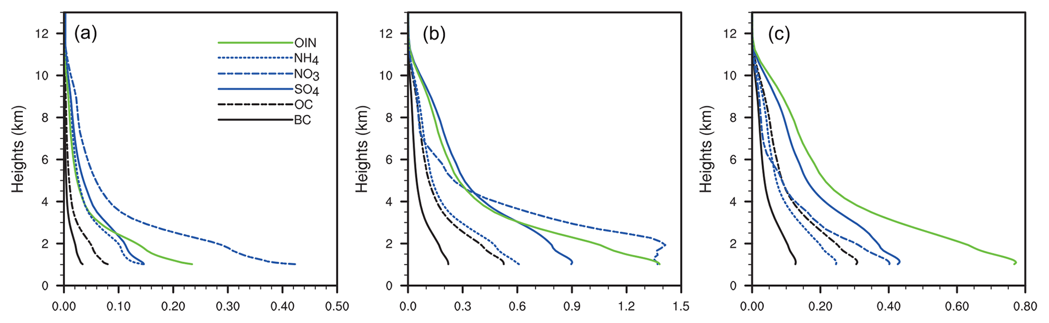
Figure 1Domain-averaged standard deviations of the background errors (µg kg−1) as a function of the height for each aerosol variable in three bins: (a) Bin 1 – 0.039–0.1 µm, (b) Bin 2 – 0.1–1.0 µm, and (c) B in 3 – 1.0–2.5 µm.
The model domain with a 40 km horizontal grid spacing covers most of China and the surrounding regions (Fig. 2), and there are 57 vertical levels extending from the surface to 10 hPa. The simulation started from 20 December of the previous year; the first 11 d were treated as a spin-up period and were not used in our analyses.
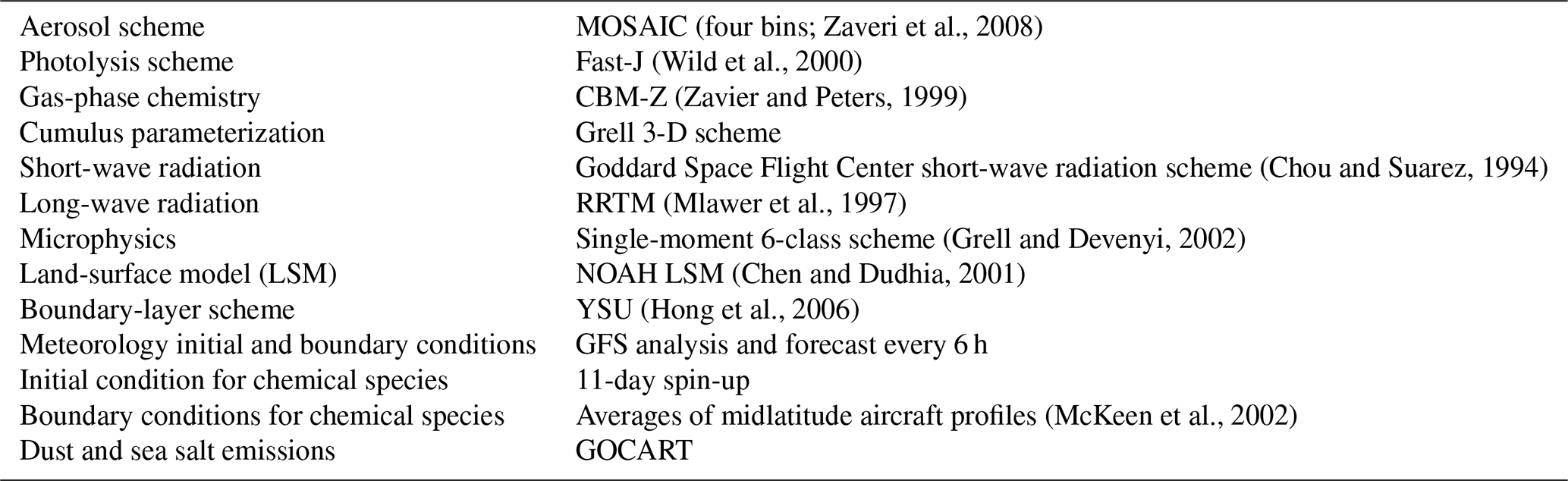
As in Chen16, the Multi-resolution Emission Inventory for China (MEIC; Zhang et al., 2009; Lei et al., 2011; He, 2012; Li et al., 2014) for January 2010 was used as the emission input, as it is the only emission inventory that was publicly available when the study was conducted. The original grid spacing of the MEIC is , and this inventory has been processed to match the model grid spacing (40 km). The spatial distributions of primary PM2.5, SO2, NOx and NH3 emissions are shown in Fig. 2. The Multi-resolution Emission Inventory for China 2010 (MEIC_2010) emission inventory has already been applied in other studies (e.g., L. T. Wang et al., 2014; Zheng et al., 2015) for simulations over China in the past few years; these recent studies found that the MEIC provides reasonable estimates of total emissions but is subject to uncertainties in the spatial allocations of these emissions over small spatial scales. For our simulations, uncertainties may also arise from two other sources: the difference between the emission base year (2010) and our simulation period (2015 through 2017) and the monthly allocations. As the Chinese government has implemented strict control strategies to ensure improved air quality during the winter season since 2013, significant reductions in emissions, including primary PM and precursor compounds (SO2 and NOx) in regions with the strict implementation of these policies relative to the year 2010, are expected for our simulation period. A reduction in SO2 pollution of approximately 50 % was observed from 2012–2015 for the North China Plain from Ozone Monitoring Instrument (OMI) satellite data (Krotkov et al., 2016). National anthropogenic emission reductions of approximately 67 %, 17 % and 35 % from 2012–2017 for SO2, NOx and PM2.5, respectively, were assumed by the bottom-up emission inventory (EI) methodology (Zheng et al., 2018). However, the expansion and relocation of the energy industry caused emission increases in northwestern China (Ling et al., 2017). In addition, the uncertainties of allocated emissions in the winter season will be much larger than those in other seasons. For example, Zhi et al. (2017) conducted a village energy survey and revealed an enormous discrepancy in the amount of rural raw coal used for winter heating in northern China, implying an extreme underestimation of rural household coal consumption by the China Energy Statistical Yearbooks. These changes and uncertainties of emissions in the model would introduce errors into the NO_DA simulation. However, the inhomogeneous spatial changes and large uncertainties in seasonal allocations made it difficult to simply scale the original emission inventory for our study period.
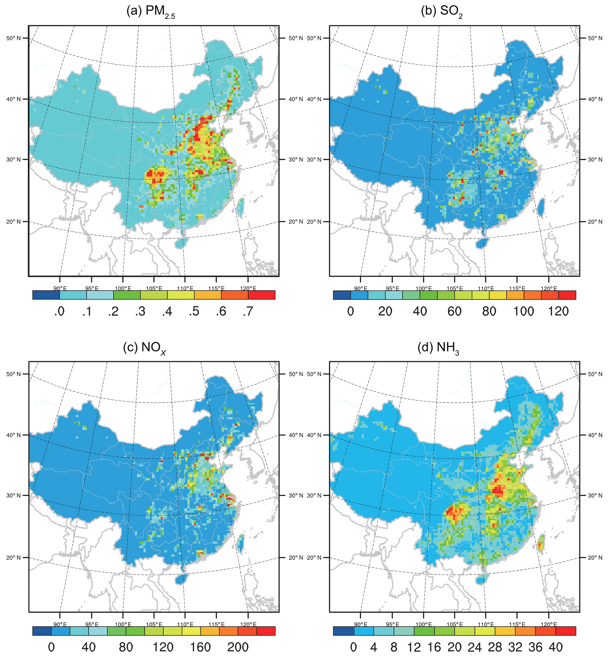
Figure 2Spatial distribution of primary PM2.5 (a; the sum of BC, OC, sulfate, nitrate and other unspecified PM2.5 emissions), SO2 (b), NOx (c) and NH3 (d) emissions (units are µg m−2 s−1 for PM2.5 and mol km−2 h−1 for the other three) used in this study.
2.2 Updated GSI 3DVAR DA system
The NCEP's GSI 3DVAR DA system was used to assimilate surface PM2.5 observations. The GSI 3DVAR DA system calculates a best-fit analysis considering the observations (hourly surface PM2.5 concentrations in our case) and background fields (a 1 h short-term WRF/Chem forecast in our case) weighted by their error characteristics. The GSI 3DVAR DA system produces an analysis in a model grid space through the minimization of a scalar objective function J(x) given by
where xb denotes the background vector (with dimension m), y is a vector of observations (with dimension p), and B and R represent the background and observation error covariance matrices with dimensions of m×m and p×p, respectively. The covariance matrices determine the relative contributions of the background and observation terms to the final analysis. H is the potentially nonlinear “observation operator” that interpolates the model grid point values into observation spaces and converts model-predicted variables into observed quantities.
2.2.1 PM2.5 observation operator
In our updated DA system, GSI was used to assimilate surface PM2.5 total mass observations, whereas the WRF/Chem model predicts the PM2.5 total mass as different prognostic variables depending on the chosen aerosol scheme. As we chose the MOSAIC-4BIN aerosol scheme, the analyzed variables here were the 3-D mass mixing ratios of the 24 MOSAIC aerosol variables at each grid point. The model-simulated PM2.5 observations were computed by summing the 24 species as
where i denotes the bin number in the MOSAIC aerosol scheme, where the first three bins consist of the PM2.5 total, and BC, OC, , , , NA, CL and OIN denote black carbon, organic compounds, sulfate, nitrate, ammonium, sodium, chloride and other inorganic compounds, respectively. This formula is identical to that used in the WRF/Chem MOSAIC scheme to diagnose PM2.5. The WRF/Chem-simulated aerosol mixing ratios of the species listed inside the brackets of Eq. (2) are in units of milligrams per kilogram, and thus the dry air density ρd is multiplied to convert the units into µg m−3 for consistency with the observations.
Since only surface PM2.5 total mass observations were assimilated to analyze the 3-D mass mixing ratios of 24 aerosol variables, the 3DVAR problem was underconstrained. Due to the lack of species and vertical information provided by the observations, the only mathematical solution is to utilize prior information from the model background. In the GSI system, the distribution of the analysis increments (the difference between the analysis and background) onto the different species was mostly driven by the model, with the observation and background error covariance matrices acting as the main constraints. This speciated approach to aerosol DA within a variational system was introduced by Liu11 and further applied by S12 and Jiang13. By using individual aerosol species as the control variables, no assumptions were made regarding the contribution of each species' mass to the total aerosol mass or to the shapes of the vertical profiles.
2.2.2 PM2.5 observations and errors
Hourly surface PM2.5 observations for January 2015–2017 were obtained from the China National Environmental Monitoring Center (CNEMC). There are more than 1600 sites in our modeling domain. As the more than 1600 monitoring sites fall into 531 model grids, all observations within the same grid are averaged (as well as the latitude and longitude) for the purpose of performing statistical calculations and evaluation. The observation sites (Fig. 3) span mostly northern, central and eastern China, while the sites are relatively sparse in western China.
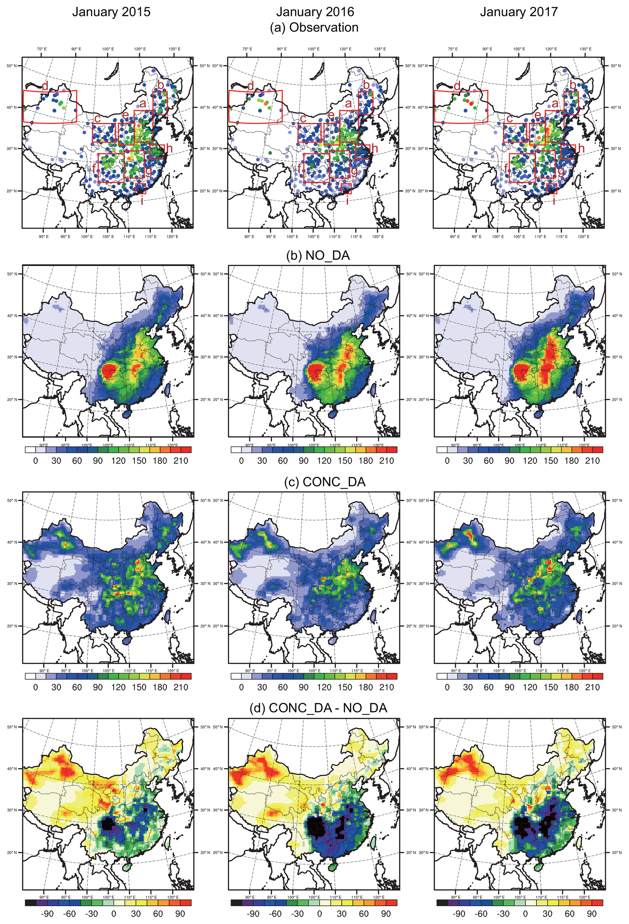
Figure 3Observed and modeled monthly average PM2.5 concentrations (unit: µg m−3) for January 2015 (left), 2016 (middle) and 2017 (right). Regions defined in red rectangles in (a) are as follows: a – NCP (North China Plain), b – NEC (northeastern China), c – EGT (Energy Golden Triangle), d – XJ (Xinjiang), e – FWP (Fenwei Plain), f – SB (Sichuan Basin), g – CC (central China), h – YRD (Yangtze River Delta) – and i – PRD (Pearl River Delta).
The observation error covariance matrix R in Eq. (1) contains both measurement and representativeness errors. Pagowski et al. (2010) used a measurement error (ε0) of 2 µg m−3. To associate higher PM2.5 values with larger measurement errors, S12 defined the measurement error as , where denotes an AIRNow PM2.5 observation and the units of each term are micrograms per cubic meter. According to the PM2.5 Auto-Monitoring Instrument Technical Standard and Requirement (China National Environmental Monitoring Center, 2013), three continuous online monitoring methods, namely, a beta ray plus dynamic heating system, a beta ray plus dynamic heating system plus light a scattering system, and a tapered element oscillating microbalance plus filter dynamic measurement system, are used at the national monitoring sites to satisfy the requirements that the display resolution should be less than 1 µg m−3, and the error should be less than 5 µg m−3 (within 24 h). To reflect the confidence in the hourly observations, the measurement error ε0 in this study is defined as , where denotes a PM2.5 observational value (unit: µg m−3).
Representativeness errors reflect the inaccuracies in the forward operator and in the interpolation from the model grid to the observation location. Elbern et al. (2007), Pagowski et al. (2010), S12 and Jiang13 defined the representativeness error (εr) as
where γ is an adjustable parameter scaling ε0 (γ=0.5 was used here), Δx is the grid spacing (40 km in our case) and L is the radius of influence of an observation (set to 2 km for urban sites). These parameter settings were based on the performance of sensitivity tests. The total PM2.5 error () is defined as
which constituted the diagonal elements in the R matrix. The PM2.5 data were provided in near-real time without any data quality control. To ensure the data quality before DA, PM2.5 observational values larger than 1000 µg m−3 (the maximum display limit of the monitoring system) were deemed unrealistic in the filter process and thus were not assimilated. In addition, observations leading to innovations and/or deviations (observations minus the model-simulated values determined from the first-guess fields) exceeding 500 µg m−3 were also omitted for the stability of the DA optimization step.
2.2.3 Background error covariance
Similar to Jiang13, the background error covariance (BEC) statistics for each analysis variable required by the 3DVAR algorithm were computed by utilizing the National Meteorological Center (NMC) method (Parrish and Derber, 1992) based on the 1 month WRF/Chem forecast for January 2015. No cross-correlation between different species was considered. The standard deviations and horizontal–vertical correlation length scales of the background errors (separated for each aerosol species) were calculated using the method described by Wu et al. (2002). These data were used as constraints for the distributions of the PM components. It is important to have phenomena-specific background error statistics to allow for an appropriate adjustment of individual species. The domain-averaged standard deviations of the background errors for six aerosol species (BC, OC, , , and OIN) in the first three size bins are shown in Fig. 1 as a function of the vertical model level; CL and NA are not shown here because they are excessively small relative to the other PM species. By using the MOSAIC aerosol scheme, the characteristics of different aerosol species in different size bins are more appropriate for the region of China in the model. As shown in Fig. 1, the standard deviations of different aerosol species errors are different in the three size bins, the errors of , OIN and are relatively larger than those of the other species in the three size bins, and OC is also important, especially in the second (0.1–1.0 µm) and third (1.0–2.5 µm) size bins. The larger background errors of those species allowed the field to be better adjusted, which was crucial for the aerosol analyses in this study.
2.3 Experimental design
We conducted two sets of experiments (NO_DA and CONC_DA) for January 2015, 2016 and 2017. In both cases, the MEIC_2010 emission inventory was used. The NO_DA experiment initialized a new WRF/Chem forecast every 6 h starting at 00:00 UTC on 20 December of the previous year to spin up the aerosol fields and was run through 23:00 UTC on 31 January. Only the simulations in January were used for the analysis. In the NO_DA experiment, the chemical and aerosol fields were simply carried over from cycle to cycle (similar to a continuous aerosol forecast), while the meteorological initial condition/boundary condition (IC/BC) were updated from GFS analysis data every 6 h to prevent the meteorological simulation from drifting. For CONC_DA, the GSI 3DVAR system updated the MOSAIC aerosol variables every hour starting from 00:00 UTC on 1 January. The background of the first cycle at 00:00 UTC on 1 January was obtained from the NO_DA experiment, and all subsequent cycles were derived from the previous cycle's 1 h forecast. In CONC_DA, the GFS analysis data were interpolated from a 6 h frequency to a 1 h frequency and were then used to update the meteorological IC/BC in each 1 h cycle. The newly added heterogeneous reactions were activated in both sets of experiments.
2.4 Distinguishing the impacts of meteorological conditions and emissions
As introduced in Sect. 1, interannual air quality changes are strongly influenced by both emissions and meteorological conditions. It is challenging to distinguish and quantify the impacts of these two aspects solely based on observations or modeling. In our case, the impacts of meteorological conditions are diagnosed by analyzing the differences between two sets of modeling simulations (with the same emission inventory but different meteorology conditions). For NO_DA, the emission inputs for January of the 3 years (2015–2017) were all from the MEIC_2010 emission inventory, and the only differences among the simulations of these 3 months were the meteorological conditions, which were acquired from the GFS 6 h analysis data. Therefore, we can assume that the differences in the simulated NO_DA PM2.5 concentrations in the 3 months were driven purely by differences in the meteorological conditions (similar to Xu et al., 2017). However, it is difficult to distinguish the impacts of emissions by using the same approach. As temporary emission control measures were applied according to the pollution severity (alarm level), the emission reduction ratios actually continued to change during the winter season; thus, no exact emission reduction ratios were provided for those days. Nevertheless, the simulation approach with different emission scenarios is simply impossible when lacking exact emission reduction ratios. Instead, we subtracted the meteorological effects from the total effects by utilizing the reanalysis data and pure model simulations. The CONC_DA result, in which the hourly surface PM2.5 observations from 531 groups of sites were utilized, can be treated as a reanalysis dataset that reflects the actual conditions (very close to the observations). Therefore, the differences in the assimilated CONC_DA PM2.5 concentrations in the 3 months reflect the combined effects of both meteorological conditions and emissions. As the two experiments were generated on gridded aerosol fields, we can separate the effects of emissions from the collective effect by subtracting the NO_DA differences from the CONC_DA differences. Hence, we can better comprehend how meteorological conditions and emissions play different roles in driving the changes in the 3 years. Table 2 illustrates this approach by taking 2015 and 2016 as an example. However, some uncertainties might be associated with this approach, as discussed in detail in Sect. 4.2.
Table 2The approach used to distinguish the different impacts of meteorological conditions and emissions by calculating them from different scenarios (taking 2015 and 2016 as an example).

This section presents the results from the NO_DA and assimilation experiments outlined above. In slight contrast to S12 and Jiang13, our purpose was to reproduce the spatio-temporal variations in the surface PM2.5 within the reanalysis dataset rather than to provide the inorganic carbon (IC) of aerosol fields for improving forecasts.
Figure 3 shows the observed and modeled monthly averages of the surface PM2.5 for January 2015, 2016 and 2017. Nine regions are illustrated as rectangles in the figure: the North China Plain (NCP), northeastern China (NEC), the Energy Golden Triangle (EGT), Xinjiang (XJ), the Fenwei Plain (FWP), the Sichuan Basin (SB), central China (CC), the Yangtze River Delta (YRD) and the Pearl River Delta (PRD). Both the observations and the model show that high values are mostly observed in NCP, FWP, SB and CC. In the NO_DA case, the model results are overpredicted in SB, NCP and CC for all 3 months, while the overestimations are more severe in SB. The NO_DA case generally overestimates (underestimates) the surface PM2.5 in NCP, SB and CC (XJ and FWP) in the 3 years, potentially indicating that the 2010 emissions are not appropriate for the 2015–2017 simulations with overestimations (underestimations). As discussed in Sect. 2.1, the large area of overestimation is consistent with the national reductions in SO2, NOx and PM2.5 anthropogenic emissions (Zheng et al., 2018); however, the underestimations in XJ and FWP also indicate the introduction of new emission sources to these two regions.
Compared to the NO_DA case, the CONC_DA assimilation experiment effectively reproduces the spatial distribution of surface PM2.5 for the 3 months in terms of the relatively higher values observed in NCP, SB and CC and in some “hotspots” (NEC, FWP and XJ), which are closer to the observations.
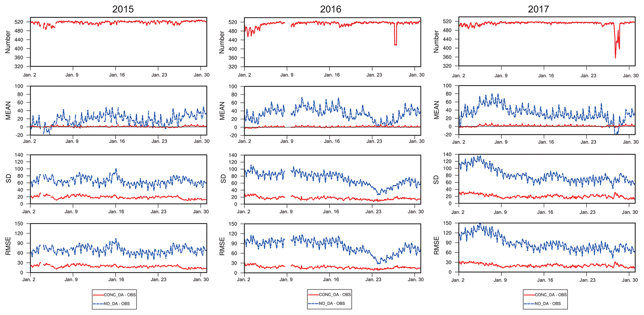
Figure 4Time series of the statistics between the model simulations and observations. Red lines are CONC_DA minus observations, and blue lines are NO_DA minus observations. Statistics include the number of data pairs for comparison, the MEAN (mean bias), the SD (standard deviation) and the RMSE (root-mean-square error). On the left is 2015, in the middle is 2016 and on the right is 2017 (units are µg m−3 for MEAN, SD and RMSE).
Basic statistical measures, including the bias (BIAS), standard deviation (SD), root-mean-square error (RMSE) and correlation coefficient (CORR), were applied to evaluate the experiments. Figure 4 shows the time series of the BIAS, SD and RMSE for all the data used in the entire domain. The statistics were calculated for each 1 h DA cycle. After quality control, the number of PM2.5 observations used in the DA process differed; the number of observations was normally approximately 500–520 but reached a minimum of 320–450 occasionally due to the data availability. From the time series, we can see that the BIAS, SD and RMSE are greatly improved in the CONC_DA case. The maximum BIAS values are approximately 50 µg m−3 for January 2015 and approximately 80 µg m−3 for 2016 and 2017 in NO_DA, while they are reduced to approximately ±5 µg −3 in CONC_DA. The SD and RMSE are also reduced by at least 50 % most of the time.
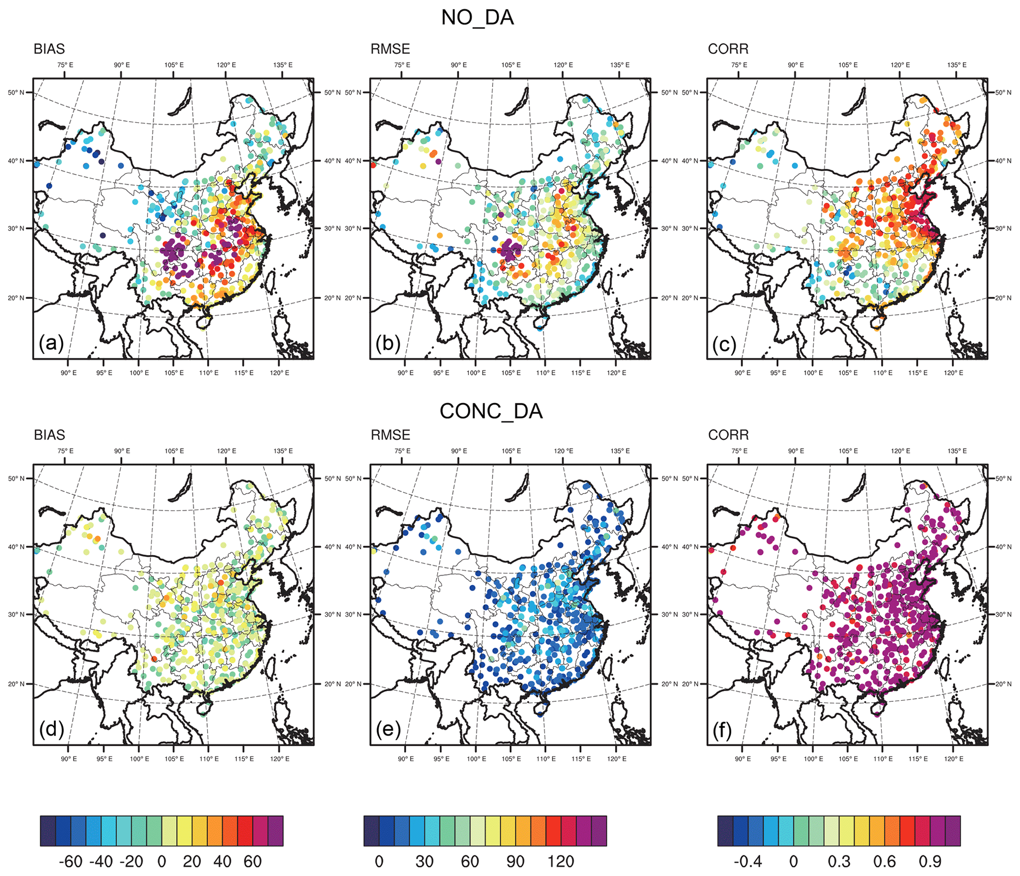
Figure 5Spatial distributions of the statistics between the model simulations and observations for January 2015. On the top is NO_DA vs. observations, and on the bottom is CONC_DA vs. observations. BIAS is the model minus observation (a, d), RMSE is the root-mean-square error (b, e) and CORR is the correlation coefficient (c, f; units are µg m−3 for BIAS and RMSE).
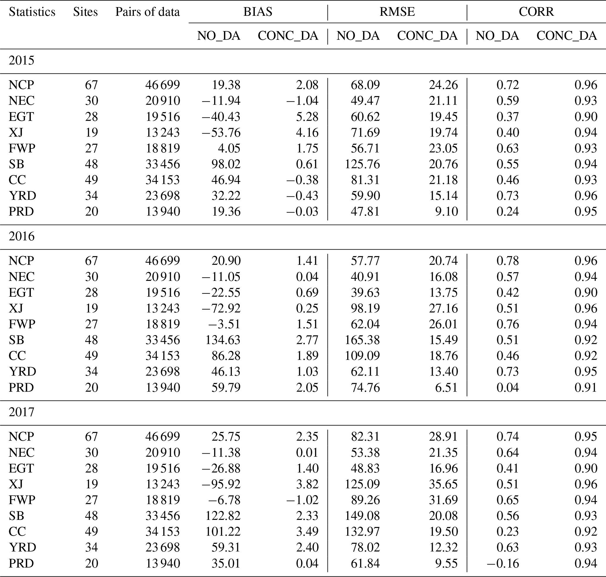
Figure 5 shows the spatial distributions of the error statistics (BIAS, RMSE and CORR) at each observational site (with more than two-thirds valid data in the month) in January 2015, 2016 and 2017. We start with 2015 and then address the differences with comparisons in 2016 and 2017. In 2015 in the NO_DA case, the surface PM2.5 concentrations are generally overestimated by 20–60 µg m−3 in eastern China (NCP, SB, CC, PRD and YRD) but are underestimated in NEC, FWP, EGT and especially XJ. The high and low BIAS values in eastern and western China are greatly corrected in CONC_DA. Consistent with the BIAS changes in CONC_DA, the RMSE and CORR distributions in eastern China and NEC are also greatly improved; the RMSE is reduced by at least 50 %, and the CORR increases to almost above 0.8–0.9. The inhomogeneous distributions of the BIAS in NO_DA in 2016 and 2017 are very similar to those in 2015 (overestimated in eastern China but underestimated in NEC, EGT and XJ). However, the high biases in CC and PRD and the low biases in XJ are even larger in 2016 and 2017. Similar to the comparisons between NO_ DA and CONC_DA for the year 2015, improvements are generally achieved for almost all the regions in both 2016 and 2017. The statistics for the nine regions are listed in Table 3.
Table 3Statistics of the observed and model-simulated surface PM2.5 for January 2015, 2016 and 2017 in nine regions (units are µg m−3 for BIAS and RMSE).
Given reliable PM2.5 reanalysis fields produced by assimilating surface PM2.5 (CONC_DA), the changes in the 3 years can be analyzed for not only scattered observational sites but also for different regions. To distinguish the roles of meteorological conditions and emissions in driving these changes, an analysis based on the NO_DA and CONC_DA simulations is performed. As assumed in Sect. 2.4, meteorology-driven changes can be analyzed in the NO_DA simulations with different meteorological conditions but the same emission inventory for different years; however, the changes in the reanalysis data in different years are actually the combination of all the driving forces, including meteorological conditions and emissions. By analyzing both sets of simulations, we can attempt to distinguish the roles of meteorology and emissions in determining these changes.
4.1 Spatial distribution
The monthly mean PM2.5 differences for January in the 3 years (2015–2017) are shown in Fig. 6 in terms of the surface concentrations measured at observational sites (Fig. 6a) and those from assimilation experiments (Fig. 6b). The surface observations are mostly reduced from 2015 to 2016, except for a few sites in the southern parts of NCP and FWP and in XJ. For the changes from 2016 to 2017, the surface observations increase at almost all the sites, especially at the sites in the southern part of NCP; the only exceptions are the sites along the coastline in YRD. The assimilated (CONC_DA) differences are consistent with the surface observations insomuch that the decreasing trend from 2015 to 2016 and the increasing trend from 2016 to 2017 for most of the regions are reproduced. However, for the changes in Tibet, EGT and XJ, where observational sites are sparse, some “cold spots” were artificially generated by CONC_DA due to the scarcity of data and the horizontal length scale set in the assimilation. As already shown in Fig. 3 and indicated here again, January 2016 is the cleanest month in the 3 years.

Figure 6Observed and modeled ambient PM2.5 concentration changes for January 2016–2015 (left), 2017–2016 (middle) and 2017–2015 (right); (a) observations, (b) assimilated total changes, (c) modeled changes due to meteorological conditions and (d) calculated changes due to emissions (units: µg m−3).
4.2 The roles of meteorological conditions and emissions
The surface PM2.5 concentrations from both the observations and the assimilation experiments show decreases from 2015 to 2016 but increases from 2016 to 2017 for most of the regions in eastern China (Fig. 6). The Chinese government has been implementing a strict emission control strategy since 2013, especially in northern China; thus, emission reductions are expected for each year following 2013. The ambient response from 2015–2017 is contradictory if considering only the reductions in emissions and omitting the changes in meteorological conditions. There are two possible assumptions: the first is that the emission reduction target was not achieved from 2016 to 2017, and the second is that other factors in addition to emissions played more important roles.
Table 4Modeled ambient PM2.5 concentration changes for 2016–2015, 2017–2016 and 2017–2015 in nine regions, and the contributions of the meteorology (MET) and emissions (EMIS) calculated according to Table 2 (units: µg m−3).
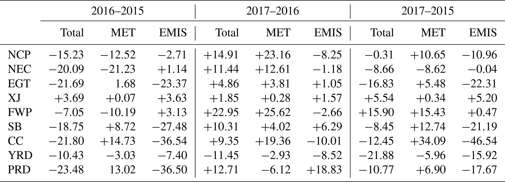
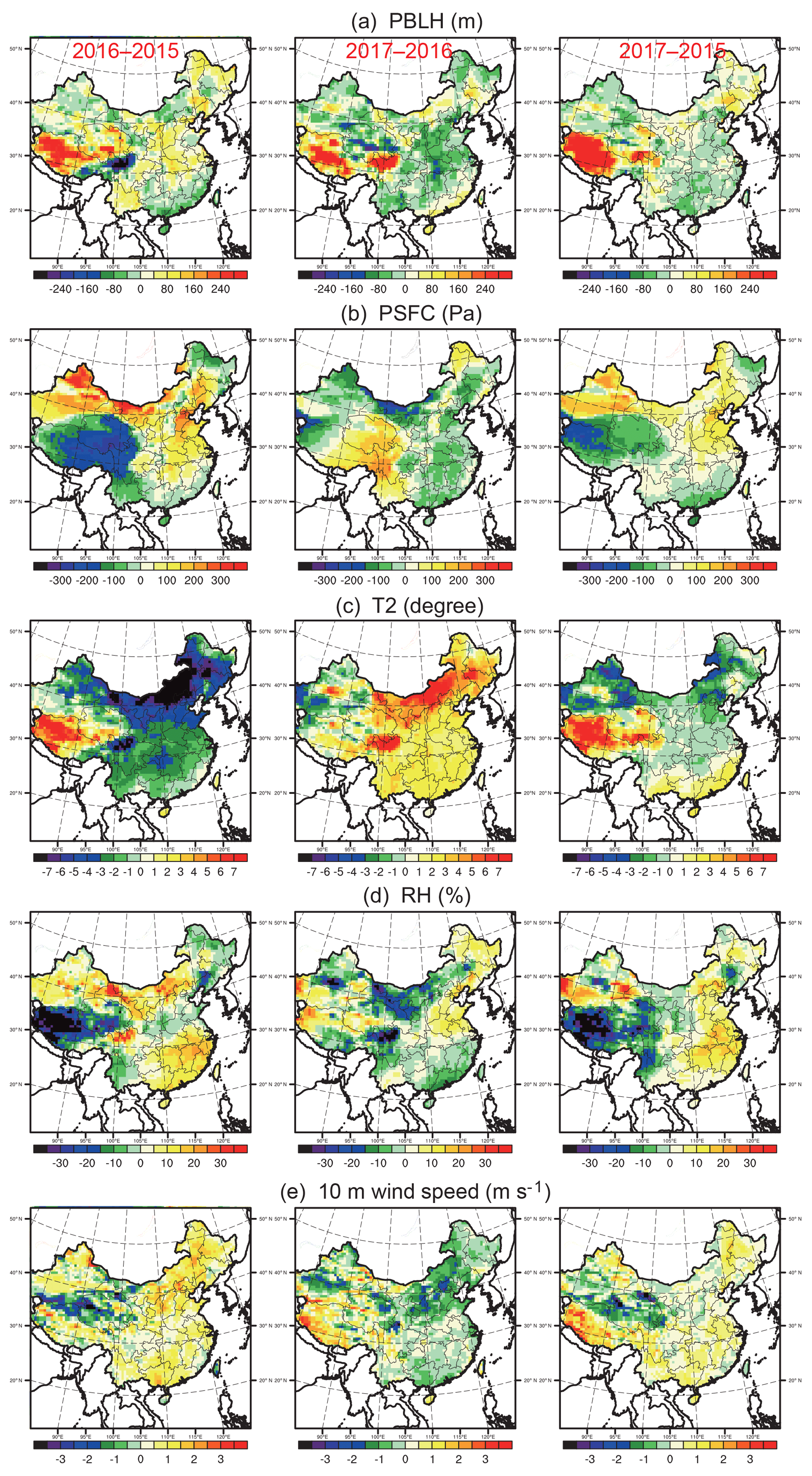
Figure 7Modeled meteorological changes for 2016–2015 (left), 2017–2016 (middle) and 2017–2015 (right). (a) PBLH, (b) PSFC, (c) T2, (d) RH2 and (e) 10 m wind speed.
The NO_DA differences in the different years are shown in Fig. 6c, which reflects the effect of meteorological condition changes (Sect. 2.4). The effect due to emissions (the other major factor in addition to meteorological conditions) is given by subtracting the NO_DA differences from the CONC_DA differences (Fig. 6d). We can clearly see that the meteorology played two different roles from 2016 to 2017. It caused a decrease in the ambient concentrations for northern China (NCP and NEC) from 2015 to 2016 but induced a large increase for northern and central China (CC) from 2016 to 2017. This indicates that the meteorological conditions might have differed from 2016 to 2017. After considering the impacts of meteorological conditions, those of emission reductions are still confirmed for these two regions from 2016 to 2017. The contributions from both meteorological conditions and emissions in the nine regions (defined in Fig. 3) were calculated, and the results are listed in Table 4. The calculations show a reduction of approximately 15–20 µg m−3 in PM2.5 for the month of January from 2015 to 2016 in northern China (NCP and NEC), but the meteorology played a dominant role (contributing a reduction of approximately 12–21 µg m−3 in PM2.5). The changes from 2016 to 2017 in NCP and NEC are completely different; meteorological conditions caused an increase in PM2.5 of approximately 12–23 µg m−3, and emission control measures caused a decrease of 1–8 µg m−3 in PM2.5, while the combined effects still showed a PM2.5 increase for that region. It is reasonable to say that emissions were indeed reduced for the northern regions from 2016 to 2017. However, the meteorology played an important role in offsetting those emission reductions and leading to an increase in surface concentrations in 2017.
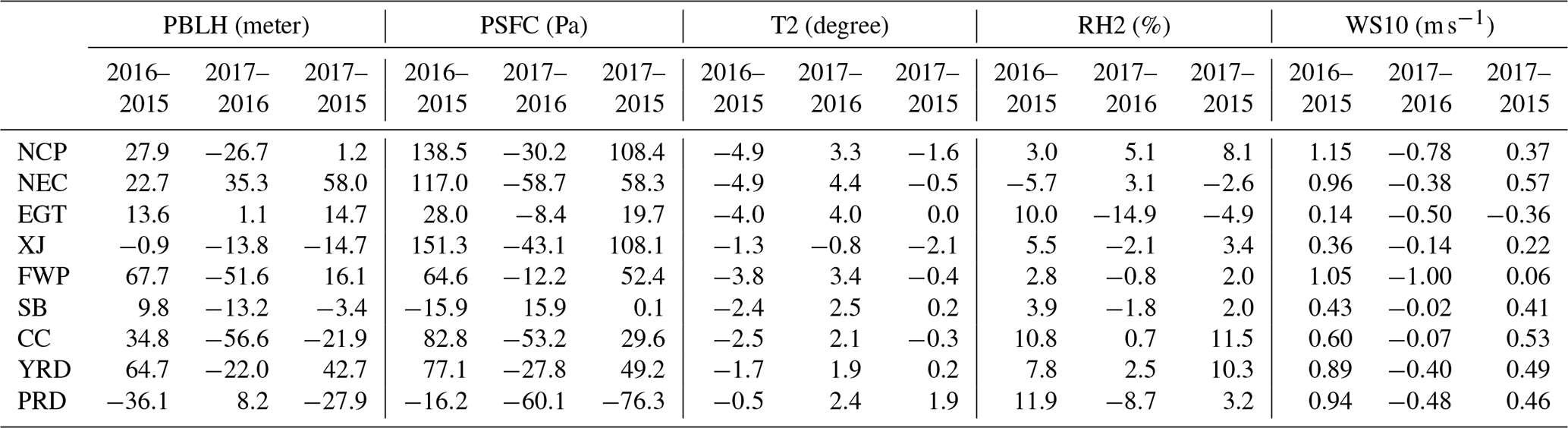
Table 5Statistics of the meteorological differences by region for January 2015, 2016 and 2017.
It is worth noting that there are uncertainties in the simulation–assimilation processes. There are three sources of uncertainties in the NO_DA simulation. First, the emission inventories in the NO_DA simulations are obviously not accurate, which may introduce uncertainties into the analysis. Although the basic assumption required only that the emissions stay the same throughout the 3 years, emission inventory uncertainty-induced errors would be offset in the subtraction process when calculating the year-to-year differences. However, it did generate uncertainties. For example, the emissions in SB, CC and PRD were generally overestimated (Fig. 3), which means that the variations in the ambient concentration might have been artificially amplified considering the meteorology impacts (Fig. 6c). In contrast, the emissions in XJ and FWP were underestimated (Fig. 3), and thus the changes in the ambient concentrations due to meteorological conditions in these two regions might have diminished. From this point of view, if the fixed emissions are more accurate in those years, the results would be more reliable. In the case where “real” emissions are not available and the purpose is to evaluate the contribution of those emissions, uncertainties are unavoidable and should be emphasized carefully. Second, the meteorological IC/BC conditions in the NO_DA simulations, which were obtained from GFS 6 h analysis data, also have uncertainties. The biases in meteorological conditions might lead to uncertainties in the PM2.5 analysis. Third, the deficiencies associated with the chemistry in the model also generate uncertainties, including missing reactions and the inaccurate parameterization of reactions. These three aspects all originate from the imperfections of current forward models. From another perspective, the accuracy of the CONC_DA assimilation experiment also affects the analysis. For example, the assimilation artificially made some “cold spots” in Tibet, EGT and XJ, where observational sites are sparse; this could also induce biases. Finally, the contribution of aerosol–meteorology feedback was not considered in our calculations. As noted by Gao et al. (2017), reduced aerosol feedbacks due to emission reductions accounted for approximately 10.9 % of the total decrease in PM2.5 concentrations in urban Beijing in their Asia-Pacific Economic Cooperation (APEC) study. In our current approach, this effect is integrated into the emissions in the subtracting process.
4.3 Meteorological changes in 2016 and 2017
It is interesting to see that meteorology played different roles in each of the 3 years. Here, we compared some meteorological parameters to explain the impacts of the meteorology. Differences in the monthly mean planetary boundary-layer height (PBLH), surface pressure (PSFC), 2 m temperature (T2), 2 m relative humidity (RH2) and 10 m wind speed in different years are given in Fig. 7. The statistics of the differences in these parameters in the nine regions are listed in Table 5, which shows that the changes in the PSFC and T2 for the periods 2015–2016 and 2016–2017 are different over the whole region. Comparing the parameters between 2015 and 2016, the pressure system is stronger, the temperature is lower and the wind speed is larger in most regions in 2016; these conditions are favorable for the dispersion of pollution. However, there are some unfavorable conditions, including a lower PBLH and a higher relative humidity (RH; and thus more heterogeneous reactions with the high RH) in northern and southern China, which may offset the impacts of high-pressure systems and low temperatures. Therefore, the combined impacts of these meteorological parameters caused a decrease in the ambient concentration in northern China and an increase in southern China from 2015 to 2016, as shown in Fig. 6. The meteorological changes are different from 2016 to 2017, with a weaker pressure system, higher temperature, smaller wind speed and lower PBLH in most regions, which caused the pollution to accumulate. As suggested by recent studies, climate change has had important impacts on extreme haze events in northern China based on historical statistical approaches or climate models. Those studies (e.g., Li et al., 2016; Zuo et al., 2015) revealed that wintertime fog–haze days across central and eastern China have a close relationship with the East Asian winter monsoon; in addition, significant weakening of the Siberian high and East Asian trough are closely correlated with warm events which boost air pollution. Consistent with our study, Zhao et al. (2018) noted that a stronger Siberian high period in January 2016 produced a significant decrease in PM2.5 concentrations relative to those during weaker periods in other years. The abovementioned studies emphasized that climate change factors and the impacts of emission changes are still difficult to evaluate. Our study used the DA technique in combination with regional models and surface observations to distinguish the impacts of emissions and meteorological conditions to further investigate the year-to-year changes at the regional scale.
To analyze the complex PM2.5 pollution in China, the GSI–WRF/Chem aerosol data assimilation system was updated from the GOCART aerosol scheme to the MOSAIC-4BIN scheme, which is more appropriate for characterizing anthropogenic emission-relevant aerosol species. Three years (2015–2017) of wintertime (January) surface PM2.5 observations from more than 1600 sites were assimilated hourly using the updated 3DVAR system in the CONC_DA assimilation experiment. A parallel control experiment that did not employ DA (NO_DA) was also performed.
Both the control and the assimilation experiments were evaluated against the surface PM2.5 observations. In the NO_DA experiment, in which the 2010_MEIC emission inventory was used, the modeled PM2.5 concentrations were severely overestimated in the Sichuan Basin (SB), central China (CC), the Yangtze River Delta (YRD) and the Pearl River Delta (PRD) by 98–134, 46–101, 32–59 and 19–60 µg m−3, respectively, which indicated that the emission estimates for 2010 are not appropriate for 2015–2017, as strict emission control strategies were implemented in recent years. Meanwhile, underestimations of 11–12, 53–96, and 22–40 µg m−3 were observed in NEC, XJ and EGT, respectively. The assimilation experiment significantly reduced the high biases of surface PM2.5 in SB, CC, YRD and PRD and the low biases in NEC and XJ with biases within ±5 µg m−3.
Both the observation and the assimilation experiments showed decreasing ambient concentrations from 2015 to 2016 but increasing concentrations from 2016 to 2017 for most of the regions. To distinguish the important factors driving these changes, the reanalysis data from the assimilation experiment and the modeling results from the control experiment were analyzed. The results showed a reduction in PM2.5 of approximately 15–20 µg m−3 for the month of January from 2015 to 2016 in northern China (NCP and NEC), but meteorology played the dominant role (contributing approximately 12–21 µg m−3 of the PM2.5 reduction). The changes from 2016 to 2017 in NCP and NEC were different; meteorological conditions caused an increase in PM2.5 of approximately 12–23 µg m−3, while emission control measures caused a decrease of 1–8 µg m−3, and the combined effects still showed a PM2.5 increase for that region. The analysis confirmed that meteorology played different roles in 2016 and 2017: the higher pressure system, lower temperatures and higher PBLH in 2016 (compared with 2015) were favorable for pollution dispersion, whereas the situation was almost the opposite in 2017 (compared with 2016) and led to an increased PM2.5 from 2016 to 2017, although emission control strategies were implemented in both years. After considering the impacts of the meteorology, the analysis showed that emissions were indeed reduced from 2015 to 2016 and 2017, especially in NCP for the year 2017 (although the surface concentrations increased that year). The analysis also showed that emissions increased in XJ and FWP.
There are still large uncertainties in this approach, such as the deficiencies of forward models (including inaccurate emission inputs, uncertainties in the meteorological IC/BC and the chemistry mechanism) and the assimilation process, and the imperfection of the aerosol–meteorology feedbacks in the model simulation generated large biases in the analysis. The most straightforward approach is thus to directly estimate the emissions by data assimilation, which will be the topic of a separate study.
The observational data is public available from http://www.cnemc.cn, last access: 7 May 2019. The simulation data may be obtained from the corresponding author upon request.
The supplement related to this article is available online at: https://doi.org/10.5194/acp-19-7409-2019-supplement.
ZL and DC designed research, DC performed research, JB contributed towards development of DA system, MC provided funds, PZ provided observational data, and DC wrote the paper, with contributions from all co-authors.
The authors declare that they have no conflict of interest.
This work was supported by the National Key R&D Program on Monitoring, Early Warning and Prevention of Major Natural Disasters under grant 2017YFC1501406, the National Natural Science Foundation of China (grant no. 41807312), and the Basic R&D special fund for central scientific research institutes (IUMKYSZHJ201701). NCAR is sponsored by the US National Science Foundation.
This research has been supported by the National Key R&D Program on Monitoring, Early Warning and Prevention of Major Natural Disasters (grant no. 2017YFC1501406), the National Natural Science Foundation of China (grant no. 41807312), and the Basic R&D special fund for central-level scientific research institutes (grant no. IUMKYSZHJ201701).
This paper was edited by Chul Han Song and reviewed by two anonymous referees.
Chen, D., Liu, Z., Fast, J., and Ban, J.: Simulations of sulfate–nitrate–ammonium (SNA) aerosols during the extreme haze events over northern China in October 2014, Atmos. Chem. Phys., 16, 10707–10724, https://doi.org/10.5194/acp-16-10707-2016, 2016.
Chen, F. and Dudhia, J.: Coupling an advanced land surface-hydrology model with the Penn State-NCAR MM5 modeling system. Part I: Model implementation and sensitivity, Mon. Weather Rev., 129, 569–585, 2001.
Cheng, Y., Zheng, G., Wei, C., Mu, Q., Zheng, B., Wang, Z., Gao, M., Zhang, Q., He, K., Carmichael, G., Poschl, U., and Su, H.: Reactive nitrogen chemistry in aerosol water as a source of sulfate during haze events in China, Sci. Adv., 2, e1601530, https://doi.org/10.1126/sciadv.1601530, 2016.
Chin, M., Savoie, D. L., Huebert, B. J., Bandy, A. R., Thornton, D. C., Bates, T. S., Quinn, P. K., Saltzman, E. S., and De Bruyn, W. J.: Atmospheric sulfur cycle simulated in the global model GOCART: Comparison with field observations and regional budgets, J. Geophys. Res.-Atmos., 105, 24689–24712, https://doi.org/10.1029/2000jd900385, 2000.
Chin, M., Ginoux, P., Kinne, S., Torres, O., Holben, B. N., Duncan, B. N., Martin, R. V., Logan, J. A., Higurashi, A., and Nakajima, T.: Tropospheric aerosol optical thickness from the GOCART model and comparisons with satellite and Sun photometer measurements, J. Atmos. Sci., 59, 461–483, https://doi.org/10.1175/1520-0469(2002)059<0461:Taotft>2.0.Co;2, 2002.
China National Environmental Monitoring Center: Ambient Air Quality Monthly Report 2015-01/2016-01/2017-01, available at: http://www.cnemc.cn/jcbg/kqzlzkbg/, last access: 17 May 2019.
China National Environmental Monitoring Center: PM2.5 Auto-Monitoring Instrument Technical Standard and Requirement, Beijing, 2013.
Chou, M.-D. and Suarez, M. J.: An efficient thermal infrared radiation parameterization for use in general circulation models, NASA Tech. Memo., TM 104606, vol. 3, 25 pp., NASA Goddard Space Flight Cent., Greenbelt, Md., 1994.
Collins, W. D., Rasch, P. J., Eaton, B. E., Khattatov, B. V., Lamarque, J. F., and Zender, C. S.: Simulating aerosols using a chemical transport model with assimilation of satellite aerosol retrievals: Methodology for INDOEX, J. Geophys. Res.-Atmos., 106, 7313–7336, https://doi.org/10.1029/2000jd900507, 2001.
Elbern, H., Strunk, A., Schmidt, H., and Talagrand, O.: Emission rate and chemical state estimation by 4-dimensional variational inversion, Atmos. Chem. Phys., 7, 3749–3769, https://doi.org/10.5194/acp-7-3749-2007, 2007.
Fast, J. D., Gustafson, W. I., Easter, R. C., Zaveri, R. A., Barnard, J. C., Chapman, E. G., Grell, G. A., and Peckham, S. E.: Evolution of ozone, particulates, and aerosol direct radiative forcing in the vicinity of Houston using a fully coupled meteorology-chemistry-aerosol model, J. Geophys. Res.-Atmos., 111, D21305, https://doi.org/10.1029/2005jd006721, 2006.
Gao, M., Liu, Z., Wang, Y., Lu, X., Ji, D., Wang, L., Li, M., Wang, Z., Zhang, Q., and Carmichael, G. R.: Distinguishing the roles of meteorology, emission control measures, regional transport, and co-benefits of reduced aerosol feedbacks in “APEC Blue”, Atmos. Environ., 167, 476–486, https://doi.org/10.1016/j.atmosenv.2017.08.054, 2017.
Grell, G. A. and Devenyi, D.: A generalized approach to parameterizing convection combining ensemble and data assimilation techniques, Geophys. Res. Lett., 29, 1693, https://doi.org/10.1029/2002gl015311, 2002.
Grell, G. A., Peckham, S. E., Schmitz, R., McKeen, S. A., Frost, G., Skamarock, W. C., and Eder, B.: Fully coupled “online” chemistry within the WRF model, Atmos. Environ., 39, 6957–6975, https://doi.org/10.1016/j.atmosenv.2005.04.027, 2005.
Han, B., Zhang, R., Yang, W., Bai, Z., Ma, Z., and Zhang, W.: Heavy air pollution episodes in Beijing during January 2013: inorganic ion chemistry and source analysis using Highly Time-Resolved Measurements in an urban site, Atmos. Chem. Phys. Discuss., 15, 11111–11141, https://doi.org/10.5194/acpd-15-11111-2015, 2015.
He, K. B.: Multi-resolution emission Inventory for China (MEIC): model framework and 1990–2010 anthropogenic emissions, Presented on the international Global Atmospheric Chemistry Conference, 17–21 September, Beijing, China, 2012.
Hong, C., Zhang, Q., He, K., Guan, D., Li, M., Liu, F., and Zheng, B.: Variations of China's emission estimates: response to uncertainties in energy statistics, Atmos. Chem. Phys., 17, 1227–1239, https://doi.org/10.5194/acp-17-1227-2017, 2017.
Hong, S. Y., Noh, Y., and Dudhia, J.: A new vertical diffusion package with an explicit treatment of entrainment processes, Mon. Weather Rev., 134, 2318–2341, 2006.
Jiang, Z., Liu, Z., Wang, T., Schwartz, C. S., Lin, H.-C., and Jiang, F.: Probing into the impact of 3DVAR assimilation of surface PM10 observations over China using process analysis, J. Geophys. Res.-Atmos., 118, 6738–6749, https://doi.org/10.1002/jgrd.50495, 2013.
Krotkov, N. A., McLinden, C. A., Li, C., Lamsal, L. N., Celarier, E. A., Marchenko, S. V., Swartz, W. H., Bucsela, E. J., Joiner, J., Duncan, B. N., Boersma, K. F., Veefkind, J. P., Levelt, P. F., Fioletov, V. E., Dickerson, R. R., He, H., Lu, Z., and Streets, D. G.: Aura OMI observations of regional SO2 and NO2 pollution changes from 2005 to 2015, Atmos. Chem. Phys., 16, 4605–4629, https://doi.org/10.5194/acp-16-4605-2016, 2016.
Liu, J., Han, Y., Tang, X., Zhu, J., and Zhu, T.: Estimating adult mortality attributable to PM2.5 exposure in China with assimilated PM2.5 concentrations based on a ground monitoring network, Sci. Total Environ., 568, 1253–1262, 2016.
Liu, Z. Q., Liu, Q. H., Lin, H. C., Schwartz, C. S., Lee, Y. H., and Wang, T. J.: Three-dimensional variational assimilation of MODIS aerosol optical depth: Implementation and application to a dust storm over East Asia, J. Geophys. Res.-Atmos., 116, D23206, https://doi.org/10.1029/2011jd016159, 2011.
Lei, Y., Zhang, Q., He, K. B., and Streets, D. G.: Primary anthropogenic aerosol emission trends for China, 1990–2005, Atmos. Chem. Phys., 11, 931–954, https://doi.org/10.5194/acp-11-931-2011, 2011.
Li, M., Zhang, Q., Streets, D. G., He, K. B., Cheng, Y. F., Emmons, L. K., Huo, H., Kang, S. C., Lu, Z., Shao, M., Su, H., Yu, X., and Zhang, Y.: Mapping Asian anthropogenic emissions of non-methane volatile organic compounds to multiple chemical mechanisms, Atmos. Chem. Phys., 14, 5617–5638, https://doi.org/10.5194/acp-14-5617-2014, 2014.
Li, Q., Zhang, R. H., and Wang, Y.: Interannual variation of the wintertime fog-haze days across central and eastern China and its relation with East Asian winter monsoon, Int. J. Climatol., 36, 346–354, https://doi.org/10.1002/joc.4350, 2016.
Li, G., Bei, N., Cao, J., Huang, R., Wu, J., Feng, T., Wang, Y., Liu, S., Zhang, Q., Tie, X., and Molina, L. T.: A possible pathway for rapid growth of sulfate during haze days in China, Atmos. Chem. Phys., 17, 3301–3316, https://doi.org/10.5194/acp-17-3301-2017, 2017.
Ling, Z., Huang, T., Zhao, Y., Li, J., Zhang, X., Wang, J., Lian, L., Mao, X., Gao, H., and Ma, J.: OMI-measured increasing SO2 emissions due to energy industry expansion and relocation in northwestern China, Atmos. Chem. Phys., 17, 9115–9131, https://doi.org/10.5194/acp-17-9115-2017, 2017.
McKeen, S. A., Wotawa, G., Parrish, D. D., Holloway, J. S., Buhr, M. P., Hubler, G., Fehsenfeld, F. C., and Meagher, J. F.: Ozone production from Canadian wildfires during June and July of 1995, J. Geophys. Res.-Atmos., 107, 4192, https://doi.org/10.1029/2001jd000697, 2002.
Mlawer, E. J., Taubman, S. J., Brown, P. D., Iacono, M. J., and Clough, S. A.: Radiative transfer for inhomogeneous atmospheres: RRTM, a validated correlated-k model for the longwave, J. Geophys. Res.-Atmos., 102, 16663–16682, 1997.
Moch, J. M., Dovrou, E., Mickley, L. J., Keutsch, F. N., Cheng, Y., Jacob, D. J., Jiang, J. K., Li, M., Munger, J. W., Qiao, X. H., and Zhang, Q.: Contribution of Hydroxymethane Sulfonate to Ambient Particulate Matter: A Potential Explanation for High Particulate Sulfur During Severe Winter Haze in Beijing, Geophys. Res. Lett., 45, 11969–11979, https://doi.org/10.1029/2018gl079309, 2018.
Pagowski, M., Grell, G. A., McKeen, S. A., Peckham, S. E., and Devenyi, D.: Three dimensional variational data assimilation of ozone and fine particulate matter observations: some results using the Weather Research and Forecasting-Chemistry model and Grid-point Statistical Interpolation, Q. J. Roy. Meteor. Soc., 136, https://doi.org/10.1002/qj.700, 2010.
Parrish, D. F. and Derber, J. C.: The National-Meteorological-Centers Spectral Statistical-Interpolation Analysis System, Mon. Weather Rev., 120, 1747–1763, doi:10.1175/1520-0493(1992)120<1747:Tnmcss>2.0.Co;2, 1992.
Schwartz, C. S., Liu, Z., Lin, H. C., and McKeen, S. A.: Simultaneous three-dimensional variational assimilation of surface fine particulate matter and MODIS aerosol optical depth, J. Geophys. Res.-Atmos., 117, https://doi.org/10.1029/2011JD017383, 2012.
Shao, J., Chen, Q., Wang, Y., Lu, X., He, P., Sun, Y., Shah, V., Martin, R. V., Philip, S., Song, S., Zhao, Y., Xie, Z., Zhang, L., and Alexander, B.: Heterogeneous sulfate aerosol formation mechanisms during wintertime Chinese haze events: Air quality model assessment using observations of sulfate oxygen isotopes in Beijing, Atmos. Chem. Phys. Discuss., https://doi.org/10.5194/acp-2018-1352, in review, 2019.
Sun, Y. L., Wang, Z. F., Du, W., Zhang, Q., Wang, Q. Q., Fu, P. Q., Pan, X. L., Li, J., Jayne, J., and Worsnop, D. R.: Long-term real-time measurements of aerosol particle composition in Beijing, China: seasonal variations, meteorological effects, and source analysis, Atmos. Chem. Phys., 15, 10149–10165, https://doi.org/10.5194/acp-15-10149-2015, 2015.
The Central People's Government of the People Republic of China: Guiding Opinions on Promoting the Joint Prevention and Control of Air Pollution to Improve Regional Air Quality, Beijing, 2010.
The Central People's Government of the People Republic of China: Atmospheric Pollution Prevention and Control Action Plan, 2013.
Wang, G., Zhang, R., Gomez, M. E., Yang, L., Levy Zamora, M., Hu, M., Lin, Y., Peng, J., Guo, S., Meng, J., Li, J., Cheng, C., Hu, T., Ren, Y., Wang, Y., Gao, J., Cao, J., An, Z., Zhou, W., Li, G., Wang, J., Tian, P., Marrero-Ortiz, W., Secrest, J., Du, Z., Zheng, J., Shang, D., Zeng, L., Shao, M., Wang, W., Huang, Y., Wang, Y., Zhu, Y., Li, Y., Hu, J., Pan, B., Cai, L., Cheng, Y., Ji, Y., Zhang, F., Rosenfeld, D., Liss, P. S., Duce, R. A., Kolb, C. E., and Molina, M. J.: Persistent sulfate formation from London Fog to Chinese haze, P. Natl. Acad. Sci. USA, 113, 13630–13635, https://doi.org/10.1073/pnas.1616540113, 2016.
Wang, G., Zhang, F., Peng, J., Duan, L., Ji, Y., Marrero-Ortiz, W., Wang, J., Li, J., Wu, C., Cao, C., Wang, Y., Zheng, J., Secrest, J., Li, Y., Wang, Y., Li, H., Li, N., and Zhang, R.: Particle acidity and sulfate production during severe haze events in China cannot be reliably inferred by assuming a mixture of inorganic salts, Atmos. Chem. Phys., 18, 10123–10132, https://doi.org/10.5194/acp-18-10123-2018, 2018.
Wang, L. T., Wei, Z., Yang, J., Zhang, Y., Zhang, F. F., Su, J., Meng, C. C., and Zhang, Q.: The 2013 severe haze over southern Hebei, China: model evaluation, source apportionment, and policy implications, Atmos. Chem. Phys., 14, 3151–3173, https://doi.org/10.5194/acp-14-3151-2014, 2014.
Wang, W., Maenhaut, W., Yang, W., Liu, X. D., Bai, Z. P., Zhang, T., Claeys, M., Cachier, H., Dong, S. P., and Wang, Y. L.: One-year aerosol characterization study for PM2.5 and PM10 in Beijing, Atmos. Pollut. Res., 5, 554–562, https://doi.org/10.5094/Apr.2014.064, 2014.
Wang, Y. S., Yao, L., Wang, L. L., Liu, Z. R., Ji, D. S., Tang, G. Q., Zhang, J. K., Sun, Y., Hu, B., and Xin, J. Y.: Mechanism for the formation of the January 2013 heavy haze pollution episode over central and eastern China, Sci. China Earth Sci., 57, 14–25, https://doi.org/10.1007/s11430-013-4773-4, 2014.
Wild, O., Zhu, X., and Prather, M. J.: Fast-j: Accurate simulation of in- and below-cloud photolysis in tropospheric chemical models, J. Atmos. Chem., 37, 245–282, 2000.
Wu, W. S., Purser, R. J., and Parrish, D. F.: Three-dimensional variational analysis with spatially inhomogeneous covariances, Mon. Weather Rev., 130, 2905–2916, doi:10.1175/1520-0493(2002)130<2905:Tdvaws>2.0.Co;2, 2002.
Xu, J., Chang, L., Yan, F., and He, J.: Role of climate anomalies on decadal variation in the occurrence of wintertime haze in the Yangtze River Delta, China, Sci. Total Environ., 599–600, 918–925, https://doi.org/10.1016/j.scitotenv.2017.05.015, 2017.
Yang, Y. R., Liu, X. G., Qu, Y., An, J. L., Jiang, R., Zhang, Y. H., Sun, Y. L., Wu, Z. J., Zhang, F., Xu, W. Q., and Ma, Q. X.: Characteristics and formation mechanism of continuous hazes in China: a case study during the autumn of 2014 in the North China Plain, Atmos. Chem. Phys., 15, 8165–8178, https://doi.org/10.5194/acp-15-8165-2015, 2015.
Zaveri, R. A. and Peters, L. K.: A new lumped structure photochemical mechanism for large-scale applications, J. Geophys. Res.-Atmos., 104, 30387–30415, 1999.
Zaveri, R. A., Easter, R. C., Fast, J. D., and Peters, L. K.: Model for Simulating Aerosol Interactions and Chemistry (MOSAIC), J. Geophys. Res.-Atmos., 113, D13204, https://doi.org/10.1029/2007jd008782, 2008.
Zhang, L., Shao, J., Lu, X., Zhao, Y., Hu, Y., Henze, D. K., Liao, H., Gong, S., and Zhang, Q.: Sources and Processes Affecting Fine Particulate Matter Pollution over North China: An Adjoint Analysis of the Beijing APEC Period, Environ. Sci. Technol., 50, 8731–8740, 2016.
Zhang, Q., Streets, D. G., Carmichael, G. R., He, K. B., Huo, H., Kannari, A., Klimont, Z., Park, I. S., Reddy, S., Fu, J. S., Chen, D., Duan, L., Lei, Y., Wang, L. T., and Yao, Z. L.: Asian emissions in 2006 for the NASA INTEX-B mission, Atmos. Chem. Phys., 9, 5131–5153, https://doi.org/10.5194/acp-9-5131-2009, 2009.
Zhao, S., Feng, T., Tie, X., Long, X., Li, G., Cao, J., Zhou, W., and An, Z.: Impact of Climate Change on Siberian High and Wintertime Air Pollution in China in Past Two Decades, Earth's Future, 6, 118–133, https://doi.org/10.1002/2017EF000682, 2018.
Zhao, Y., Zhou, Y. D., Qiu, L. P., and Zhang, J.: Quantifying the uncertainties of China's emission inventory for industrial sources: From national to provincial and city scales, Atmos. Environ., 165, 207–221, https://doi.org/10.1016/j.atmosenv.2017.06.045, 2017.
Zheng, B., Zhang, Q., Zhang, Y., He, K. B., Wang, K., Zheng, G. J., Duan, F. K., Ma, Y. L., and Kimoto, T.: Heterogeneous chemistry: a mechanism missing in current models to explain secondary inorganic aerosol formation during the January 2013 haze episode in North China, Atmos. Chem. Phys., 15, 2031–2049, https://doi.org/10.5194/acp-15-2031-2015, 2015.
Zheng, B., Tong, D., Li, M., Liu, F., Hong, C., Geng, G., Li, H., Li, X., Peng, L., Qi, J., Yan, L., Zhang, Y., Zhao, H., Zheng, Y., He, K., and Zhang, Q.: Trends in China's anthropogenic emissions since 2010 as the consequence of clean air actions, Atmos. Chem. Phys., 18, 14095–14111, https://doi.org/10.5194/acp-18-14095-2018, 2018.
Zhi, G. R., Zhang, Y. Y., Sun, J. Z., Cheng, M. M., Dang, H. Y., Liu, S. J., Yang, J. C., Zhang, Y. Z., Xue, Z. G., Li, S. Y., and Meng, F.: Village energy survey reveals missing rural raw coal in northern China: Significance in science and policy, Environ. Pollut., 223, 705–712, https://doi.org/10.1016/j.envpol.2017.02.009, 2017.
Zuo, Z. Y., Zhang, R. H., Huang, Y., Xiao, D., and Guo, D.: Extreme cold and warm events over China in wintertime, Int. J. Climatol., 35, 3568–3581, https://doi.org/10.1002/joc.4229, 2015.