the Creative Commons Attribution 4.0 License.
the Creative Commons Attribution 4.0 License.
 | 03 Jun 2019
Development of a versatile source apportionment analysis based on positive matrix factorization: a case study of the seasonal variation of organic aerosol sources in Estonia
Athanasia Vlachou
Anna Tobler
Houssni Lamkaddam
Francesco Canonaco
Kaspar R. Daellenbach
Jean-Luc Jaffrezo
María Cruz Minguillón
Marek Maasikmets
Erik Teinemaa
Urs Baltensperger
André S. H. Prévôt
Bootstrap analysis is commonly used to capture the uncertainties of a bilinear receptor model such as the positive matrix factorization (PMF) model. This approach can estimate the factor-related uncertainties and partially assess the rotational ambiguity of the model. The selection of the environmentally plausible solutions, though, can be challenging, and a systematic approach to identify and sort the factors is needed. For this, comparison of the factors between each bootstrap run and the initial PMF output, as well as with externally determined markers, is crucial. As a result, certain solutions that exhibit suboptimal factor separation should be discarded. The retained solutions would then be used to test the robustness of the PMF output. Meanwhile, analysis of filter samples with the Aerodyne aerosol mass spectrometer and the application of PMF and bootstrap analysis on the bulk water-soluble organic aerosol mass spectra have provided insight into the source identification and their uncertainties. Here, we investigated a full yearly cycle of the sources of organic aerosol (OA) at three sites in Estonia: Tallinn (urban), Tartu (suburban) and Kohtla-Järve (KJ; industrial). We identified six OA sources and an inorganic dust factor. The primary OA types included biomass burning, dominant in winter in Tartu and accounting for 73 % ± 21 % of the total OA, primary biological OA which was abundant in Tartu and Tallinn in spring (21 % ± 8 % and 11 % ± 5 %, respectively), and two other primary OA types lower in mass. A sulfur-containing OA was related to road dust and tire abrasion which exhibited a rather stable yearly cycle, and an oil OA was connected to the oil shale industries in KJ prevailing at this site that comprises 36 % ± 14 % of the total OA in spring. The secondary OA sources were separated based on their seasonal behavior: a winter oxygenated OA dominated in winter (36 % ± 14 % for KJ, 25 % ± 9 % for Tallinn and 13 % ± 5 % for Tartu) and was correlated with benzoic and phthalic acid, implying an anthropogenic origin. A summer oxygenated OA was the main source of OA in summer at all sites (26 % ± 5 % in KJ, 41 % ± 7 % in Tallinn and 35 % ± 7 % in Tartu) and exhibited high correlations with oxidation products of a-pinene-like pinic acid and 3-methyl-1, 2, 3-butanetricarboxylic acid (MBTCA), suggesting a biogenic origin.
- Article
(4896 KB) - Full-text XML
-
Supplement
(1346 KB) - BibTeX
- EndNote


Particulate matter of an aerodynamic diameter smaller than 10 µm (PM10) has been extensively explored at many sites around the globe due to its various adverse effects on human health and climate. In Europe, several monitoring networks have been measuring PM10 for long time periods, and an increasing trend in concentrations from north to south was noticed (Fuzzi et al., 2015; Putaud et al., 2010). Despite this, some northern European countries are still suffering from PM10 daily limit exceedances (European Environment Agency report No 13/2017, 2017), and according to modeling studies following the “current legislation” scenarios, some of these sites will remain exposed to high PM10 standards until 2030 (Kiesewetter et al., 2015). Therefore, understanding the origins of the pollutants can play a crucial role in future abatement policies.
While large efforts have been devoted to the investigation of the sources and the chemical composition of PM10, and in particular the organic fraction in western and central Europe, measurements in eastern Europe and the Baltic region are scarce. More specifically, the organic aerosol (OA) composition in Estonia has received little attention so far. PM2.5 organic aerosol source apportionment was extensively studied by Elser et al. (2016), who performed mobile lab measurements during March 2014 at two different sites, Tallinn and Tartu. They found similar sources of OA at both sites where residential biomass burning, traffic and long-range transported OA were the major sources of OA. They also found a localized residentially influenced OA factor, which was connected to cooking activities and possibly to coal and waste burning. While the long-range transported OA dominated during nighttime and during several events when polluted air masses were transported from northern Germany, the remaining factors were important during daytime. These results provided insights into the spatial resolution of OA. Nevertheless, they were limited to short time periods; hence, the seasonal variation of the pollutants remains unknown. Residential wood combustion and traffic were also presented as important sources of PM in previous long-term air pollution studies in Estonia (Urb et al., 2005; Orru et al., 2010). However, they did not provide any quantitative source apportionment for OA.
The offline aerosol mass spectrometer (AMS) technique was recently developed by Daellenbach et al. (2016), where aqueous filter extracts are measured after nebulization with an Aerodyne high-resolution time-of-flight aerosol mass spectrometer (HR-ToF-AMS; Canagaratna et al., 2007), and the resulting organic mass spectra are analyzed with positive matrix factorization (PMF; Paatero, 1997). This technique has significantly increased our capability to investigate and identify the seasonal behavior of OA sources at several sites around the globe (Huang et al., 2014; Daellenbach et al., 2017; Bozzetti et al., 2017a). In addition, this technique allows for OA measurements of different size fractions overcoming the limitation given by the transmission window of the AMS, resulting in quantifying sources from the coarse mode, such as primary (i.e., OA directly emitted in the atmosphere), biological (Bozzetti et al., 2016) or sulfur-containing primary OA sources (Daellenbach et al., 2017).
PMF is widely used to analyze ambient aerosol measurement data by decomposing the input aerosol mass spectra into factor concentration time series and factor profiles. To do so, PMF iteratively solves the bilinear Eq. (1), where Xi,j represents the measured input data matrix in which i is the number of samples and j is the chemical species measured, Gi,k represents the concentration time series matrix in which k is the number of factors, Fk,j represents the factor profile matrix, and E represents the residual matrix. The goal of PMF is to solve Eq. (1) such that the object function Q (Eq. 2) is minimized. In Eq. (2), U represents the corresponding error matrix:
Bilinear models suffer from rotational ambiguity, that is, a mathematically similar goodness of fit (Henry, 1987), leading to uncertainties in extracting the contributions of different OA sources. Additional modeling errors may occur due to the user subjectivity in analyzing natural phenomena, when, for example, selecting the number of interpretable factors or estimating the error matrix.
The bootstrap analysis (Davison and Hinkley, 1997), a resampling technique of the original data and error matrices, has been widely adopted to assess, to a certain extent, the rotational ambiguity related to PMF analysis (Brown et al., 2015). For each bootstrap iteration a random number of samples are selected with repeats from the original input matrices (base case) to recreate new input matrices with the same dimensions (bootstrap iteration) that will be analyzed with PMF. As a result, the bootstrap analysis results in a great number of solutions whose environmental representativeness has to be assessed, which requires a systematic approach in relating the separated factors to specific sources. This factor classification has been typically based on the contributions of certain markers (e.g., to identify biomass burning OA or to identify secondary OA; Daellenbach et al., 2017, 2018; Bozzetti et al., 2017a; Vlachou et al., 2018) in the case of the application of PMF to AMS data. However, in datasets with similar factor profiles, for example two oxygenated OA factors or more, this type of sorting can become challenging, especially when a bootstrap iteration does not provide the expected factors. To assess the quality of the different bootstrap solutions, users typically compare the factor time series to external marker measurements, when available, and discard suboptimal solutions using a set of acceptance criteria (Ulbrich et al., 2009; Q. Zhang et al., 2011; Norris et al., 2014; Bozzetti et al., 2017a, b; Y. L. Zhang et al., 2017).
In this study, we propose a novel technique for evaluating the selection of the PMF solutions generated through a large number of bootstrap iterations. The method is based on the examination of the correlation matrix between the base case and bootstrap iterations for both time series and profiles, without setting a priori a defined threshold in the correlation coefficient. We assess the performance of the technique (accuracy and probability of false positive and false negative results) by comparing the factors' time series to the available specific markers. We applied the technique to an unprecedented dataset of 150 PM10 filter samples from three sites in Estonia covering a full year (September 2013–September 2014), where anthropogenic and natural emissions of primary and secondary organic aerosols could be extracted.
2.1 Sampling sites
The samples were collected at three different sites in Estonia: Tallinn, Tartu and Kohtla-Järve (KJ). Tallinn is the capital and the largest city of Estonia located on the northern coast facing the Gulf of Finland. The measurement station is located about 9 km from the city center, in the sub-district Õismäe (59∘24′50.927′′ N, 24∘38′57.207′′ E; 8.5 m a.s.l.). Tartu is the second largest city of Estonia, located in the southeastern part of the country, in the valley of the Emajõgi River, a location that favors temperature inversions and the trapping of air pollutants. The measurement station (58∘22′14.183′′ N, 26∘44′5.517′′ E; 39.5 m a.s.l.) is positioned in the city center. According to Orru et al. (2010) traffic and local heating are important sources of air pollution at these sites. In both cities the fleet of cars increases in contrast to the limited street network capacity. Moreover, the local heating is more pronounced in Tartu compared to Tallinn. KJ is a coastal industrial city located in the northeastern part of Estonia (59∘24′34.513′′ N, 27∘16′43.166′′ E; 55.5 m a.s.l.). The main industries are related to large production of petroleum products, oil shale processing and electricity generation. As it is not a highly populated area, residential heating or traffic is not as important as in the other two cities.
The measurements were performed with 24 h integrated PM10 quartz fiber filter samples from KJ (31 August 2013 to 25 August 2014), Tallinn (5 September 2013 to 1 September 2014) and Tartu (5 September 2013 to 31 September 2014; see Tables S1 and S2 and Fig. S1 in the Supplement for details). PM was collected onto 15 cm diameter quartz filters, using a high volume sampler (500 L min−1). After exposure, the filter samples were wrapped in lint-free paper, sealed in polyethylene bags and stored at −20 ∘C.
2.2 Major ionic species, sugar and acid analyses
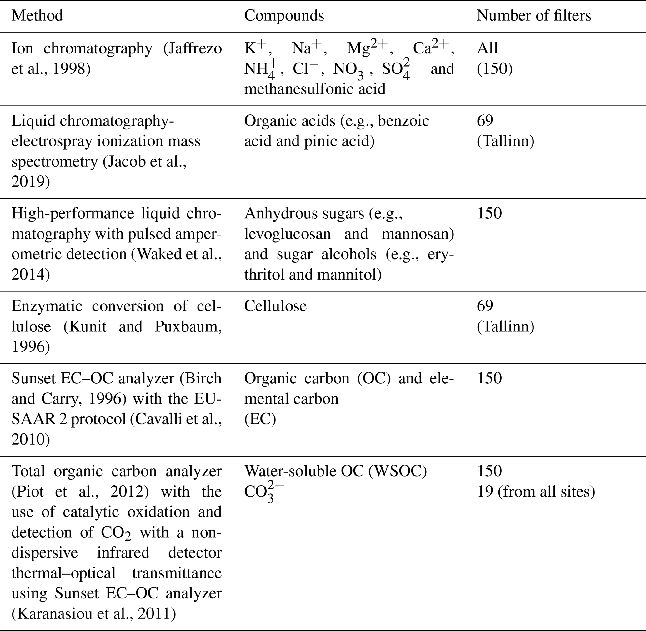
The additional filter measurements, performed to corroborate and support the source apportionment, are listed in Table 1.
2.3 Offline AMS technique
The offline AMS technique was established by Daellenbach et al. (2016) and is briefly described in the following. From each filter sample, four punches of 16 mm in diameter were extracted in 15 mL of ultrapure water (18.2 MΩ cm at 25 ∘C with total organic carbon < 3 ppb). The liquid extracts were inserted into an ultrasonic bath for 20 min at 30 ∘C. The ultrasonicated samples were then filtered through a nylon membrane syringe of 0.45 µm. Out of the resulting solutions, aerosols were generated in Ar (≥99.998 % volume, Carbagas, Gümligen, Switzerland) via an apex Q nebulizer (Elemental Scientific, Inc., Omaha, NE, USA) operating at 60 ∘C and subsequently directed into the AMS after being dried by a Nafion dryer.
The technique was performed on 150 filter samples in total: 39 from KJ, 69 from Tallinn and 42 from Tartu (Tables S1 and S2). The resulting organic spectra were analyzed by PMF with the use of the multilinear engine 2 (ME-2; Paatero, 1999). The interface for the data processing was provided by the source finder toolkit (SoFi version 4.9; Canonaco et al., 2013) for Igor Pro (WaveMetrics, Inc., Portland, Oregon, USA).
The NH4NO3 artifact on the signal (Pieber et al., 2016) was also accounted for. For a thorough description of the artifact and the correction procedure, the reader is referred to Pieber et al. (2016) and to Daellenbach et al. (2017).
2.4 PMF input and uncertainties
As stated in the introduction, the input data matrix for the PMF is the organic mass spectrum data matrix Xi,j which consists of a combination of factor profiles, and time series and the input error matrix U include the blank variability and the measurement uncertainties. Before using the PMF algorithm, all the fragments with a signal-to-noise ratio (SNR) below 0.2 were removed from the input matrix, and the ones with SNR below 2 were down weighted according to the recommendations of Paatero and Hopke (2009). Note that the PMF input matrix Xi,j included the data from all three sites.
To obtain quantitative results, both data and error matrices were multiplied by the externally measured water-soluble OC (WSOC) times the OM:OC ratio retrieved from the factor profiles of the matrix Xi,j.
Even though traffic is expected to be one of the primary sources of air pollutants, especially in Tallinn and Tartu, a clear hydrocarbon-like OA (HOA) which mainly contains non-water-soluble compounds could not be identified due the extraction procedure used. To assess a potential effect of the water-soluble HOA (WSHOA) on the PMF results, we estimate the WSHOA contribution to the different fragments in the data matrix. The calculation was based on the time series of the concentration of elemental carbon (EC) and the averaged high-resolution HOA reference factor profiles from Crippa et al. (2013) and Mohr et al. (2012) multiplied by the HOA:EC ratio (which is 0.4) reported by El Haddad et al. (2013) multiplied by the recovery RHOA=0.11 reported by Daellenbach et al. (2016; see Sect. 4 for more information on the recoveries). The calculated WSHOA data matrix was then subtracted from the original data matrix. The PMF output did not change with the subtraction of WSHOA, even though the calculated concentration of the latter was a high estimate due to the assumption that EC only originates from traffic. A thorough apportionment of EC and the calculation of HOC will be discussed in Sect. 4.1.
The variability in the AMS input dataset was best described by a seven-factor solution, which will be thoroughly described in Sect. 3.1 below. To assess the stability of the PMF solution and the sensitivity of the model for the WSHOA subtraction, we performed 250 bootstrap runs by perturbing the HOA:EC and RHOA parameters within their errors (1 standard deviation, σ), assuming a normal distribution. Note that this number of runs was restricted by computational limitations.
The sorting of the factors and the concomitant selection of the retainable solutions out of the 250 runs was based on the correlation (R Spearman – Rs) of the time series between the base case (which is the PMF result before bootstrapping) and each bootstrap iteration n as well as the correlation (Rs) of each factor profile between the base case and each iteration n. In the following, the sorting based on the time series is denoted as “ts”, and the sorting based on profiles is denoted as “pr”. The criteria, followed for the selection or rejection of each solution, are described in Sect. 3.2.
3.1 Interpretation of PMF factors
As already mentioned, the variability in the water-soluble organic mass spectra was best explained by a seven-factor solution, which we refer to as the base case. The factors found were as follows:
-
An oil-related OA was found that was rich in hydrocarbons (Fig. 1a) and showed elevated concentrations, mainly in KJ (Fig. 1b).
-
A sulfur-containing OA (SCOA) factor was found with a pronounced peak at m∕z 79 (; Fig. 1a) and rather stable contributions at all sites (Fig. 1b). As this factor was significantly enriched in the coarse mode (Vlachou et al., 2018), mainly found in urban areas influenced by traffic at other European sites (Daellenbach et al., 2017) and clearly associated with fossil carbon (Vlachou et al., 2018), we have previously related it to asphalt abrasion or tire wear.
-
A summer oxygenated OA (SOOA) was found with enhanced m∕z 43 (C3H2O+) and 44 () peaks (Fig. 1a), which was highest during summer at all sites (Fig. 1b).
-
A winter oxygenated OA (WOOA) was found with enhanced peaks at m∕z 28 (CO+) and 44 (; Fig. 1a), dominating in winter at all sites (Fig. 1b). Both of these oxygenated factors (SOOA and WOOA) were also found in different European sites and were connected to non-fossil sources, biogenic and anthropogenic, respectively (Vlachou et al., 2018; Daellenbach et al., 2018). Such a distinction was also found in Canonaco et al. (2015), where an online ACSM was used.
-
A factor with a significantly pronounced peak at m∕z 44 (; Fig. 1a) and elevated concentrations in summer (Fig. 1b) was found, which was identified as dust. This factor will be more thoroughly examined in Sect. 4.
-
A primary biological OA (PBOA) was found which exhibited high contributions of the fragment (at m∕z 61; Bozzetti et al., 2016; Fig. 1a) and increased concentrations during late spring and summer at all sites (Fig. 1b).
-
A biomass burning OA (BBOA) was found with a characteristic peak at m∕z 60 (; Alfarra et al., 2007; Fig. 1a) and elevated concentrations during late fall and winter in Tallinn and especially in Tartu (Fig. 1b).
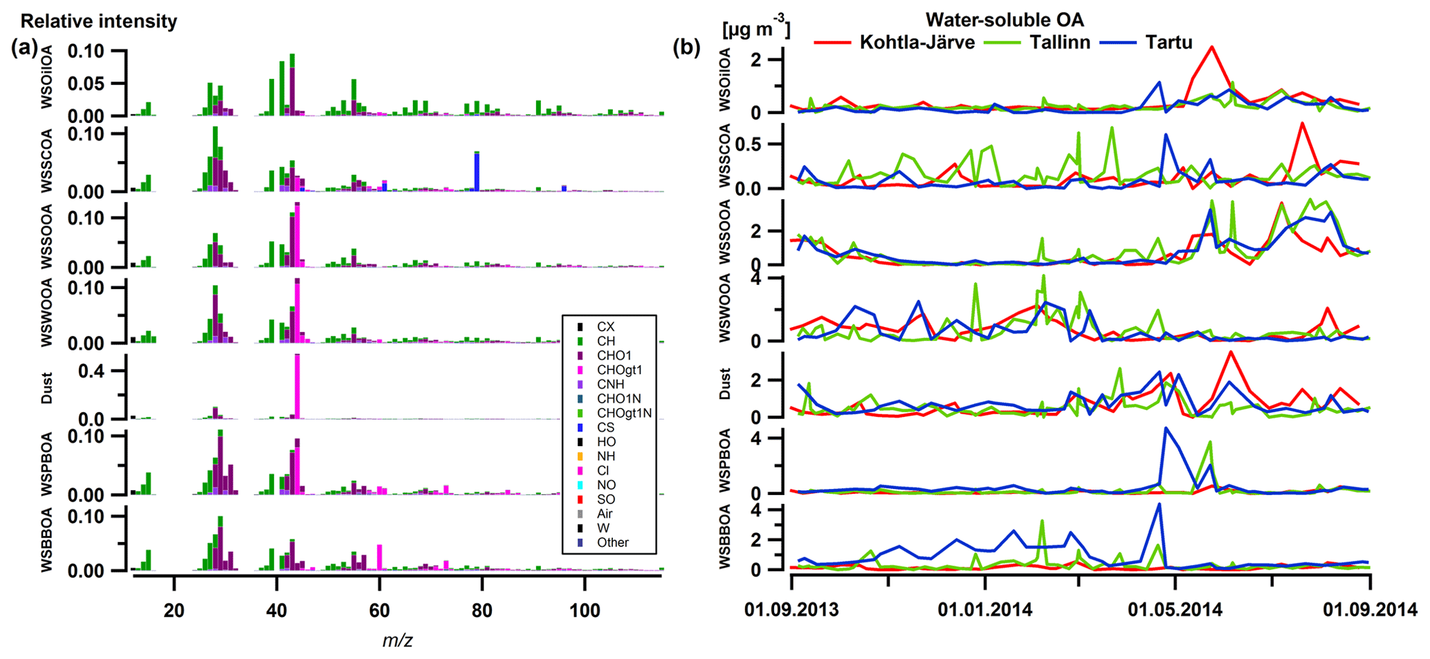
Figure 1Factor profiles (a) and time series (b) of the seven-factor solution: industrial or oil combustion OA (OilOA), sulfur-containing OA (SCOA), summer oxygenated OA (SOOA), winter oxygenated OA (WOOA), dust-related OA (Dust), primary biological OA (PBOA) and biomass burning OA (BBOA). Note that the water-soluble parts are illustrated here.
3.2 PMF uncertainty analysis: factor sorting and solution selection
The framework for factor sorting and solution selection proceeded as follows:
-
A correlation matrix was composed, including all the correlations between base-case factor time series (profiles) represented in rows and bootstrap iteration n time series (profiles) represented in columns, demonstrating the Rs per correlation (Fig. 2).
-
Factors were sorted according to the highest correlation of their time series (profiles) with the base-case factor time series (profile).
-
Solutions were discarded if any of the correlation coefficients occurring in the matrix diagonal were not statistically significantly higher than at least one of the coefficients in the respective column or row (significance level α=0.05). These selection criteria have two implications: (1) every factor separated in a bootstrap run should correspond to a unique factor of the seven factors separated in the base case, and (2) all factors that could be identified in the base case have one unambiguous corresponding factor in the bootstrap run. We have statistically evaluated the comparison between the Spearman coefficients by treating them as if they were Pearson coefficients (Myers et al., 2006) and by applying the standard Fisher's z transformation and subsequent comparison using a t test. This approach was reported to be more robust with respect to the type I error (false positive) than ignoring the non-normality and using Pearson instead of Spearman coefficients.
An example of the correlation matrix of a retained solution is shown in Fig. 2a for time series and Fig. 2b for profiles. Meanwhile, Fig. 2c and Fig. 2d represent examples of a bootstrap iteration (n=140) where the solution was rejected because SCOA was not resolved, based on both ts and pr analysis, respectively. In Fig. 2c, the highest correlation between the time series of factor 2 and the factors of the base case was found with dust instead of SCOA, yet it was much weaker (Rs=0.34) than the correlation between factor 7 and dust (Rs=0.79). Therefore, factor 7 could be identified as dust, and factor 2 could not be identified as an interpretable factor. In Fig. 2d, factor profile 2 correlated most with the base-case SCOA profile; however this correlation was not significantly higher than the correlation between factor 2 and dust. Moreover, base-case SCOA correlated better with factor 6, which was related to SOOA, indicating that SCOA could not be unambiguously related to factor 2.
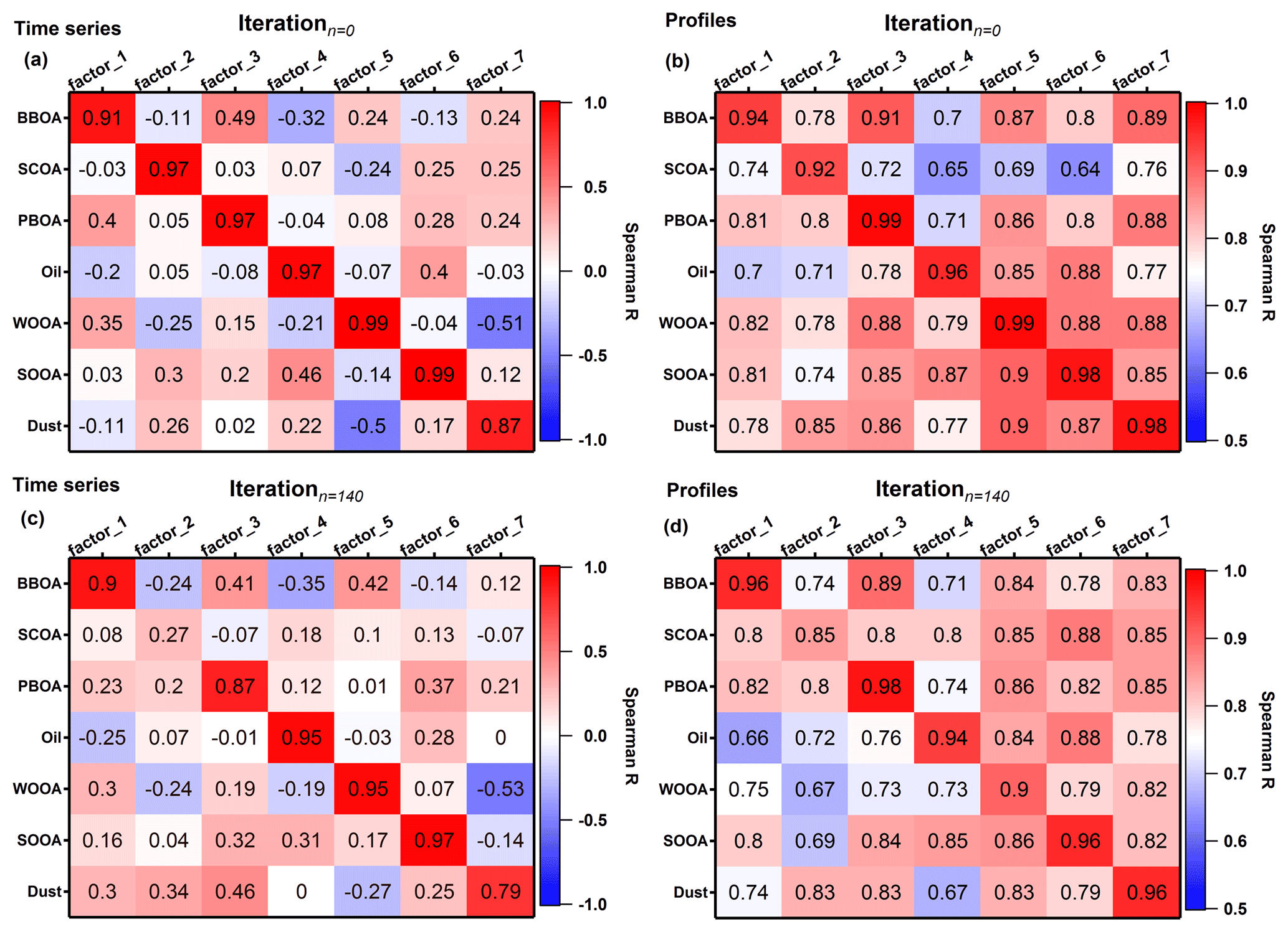
Figure 2Explanatory tables for the factor sorting based on the time series: (a) accepted bootstrap iteration where all highest correlations (Rs) lay in the diagonal, and (c) failure to resolve SCOA, as for this bootstrap iteration, both factors 2 and 7 showed the highest correlation with dust factor. The respective tables for the case of profiles are in (b) and (d). Note the different scales of Rs for the profiles.
To validate the selection of the solutions, we compared the factors of each bootstrap iteration with an externally measured marker, more specifically BBOA with levoglucosan, PBOA with cellulose, WOOA with phthalic acid and SOOA with 3-methyl-1,2,3-butanetricarboxylic acid (MBTCA). The retained solutions exhibited the highest correlations between the external markers and the respective factors (red markers in Fig. 3). To seal the validity of the retained solutions, we also compared the Rs between the base-case factors and their respective external marker with the Rs between the bootstrap iteration factors and their respective external markers. We performed the bootstrap technique for a second time on the time series of the base-case factors and the respective external markers 1000 times. The resulting Rs coefficients are represented in probability density functions (PDFs) indicated as red curves in Fig. 3, centered at 0.8 for BBOA (Fig. 3a), 0.7 for WOOA (Fig. 3c) and 0.9 for SOOA (Fig. 3d) and a broader one centered at 0.45 for PBOA (Fig. 3b). In all four cases, the retained solutions, either coming from the ts or the pr approach, spanned around the center of each PDF (Fig. 3 and Fig. S2 for the pr), and most of the solutions where at least one factor was not resolved (black markers in Fig. 3) were not included within the PDF boundaries. The general agreement between the PDFs and the retained solutions ratified the solution selection approach; however, there were still some cases of possible misallocation of retained or rejected solutions (for example, a few black markers appearing at the center of the PDF; Fig. 3c).
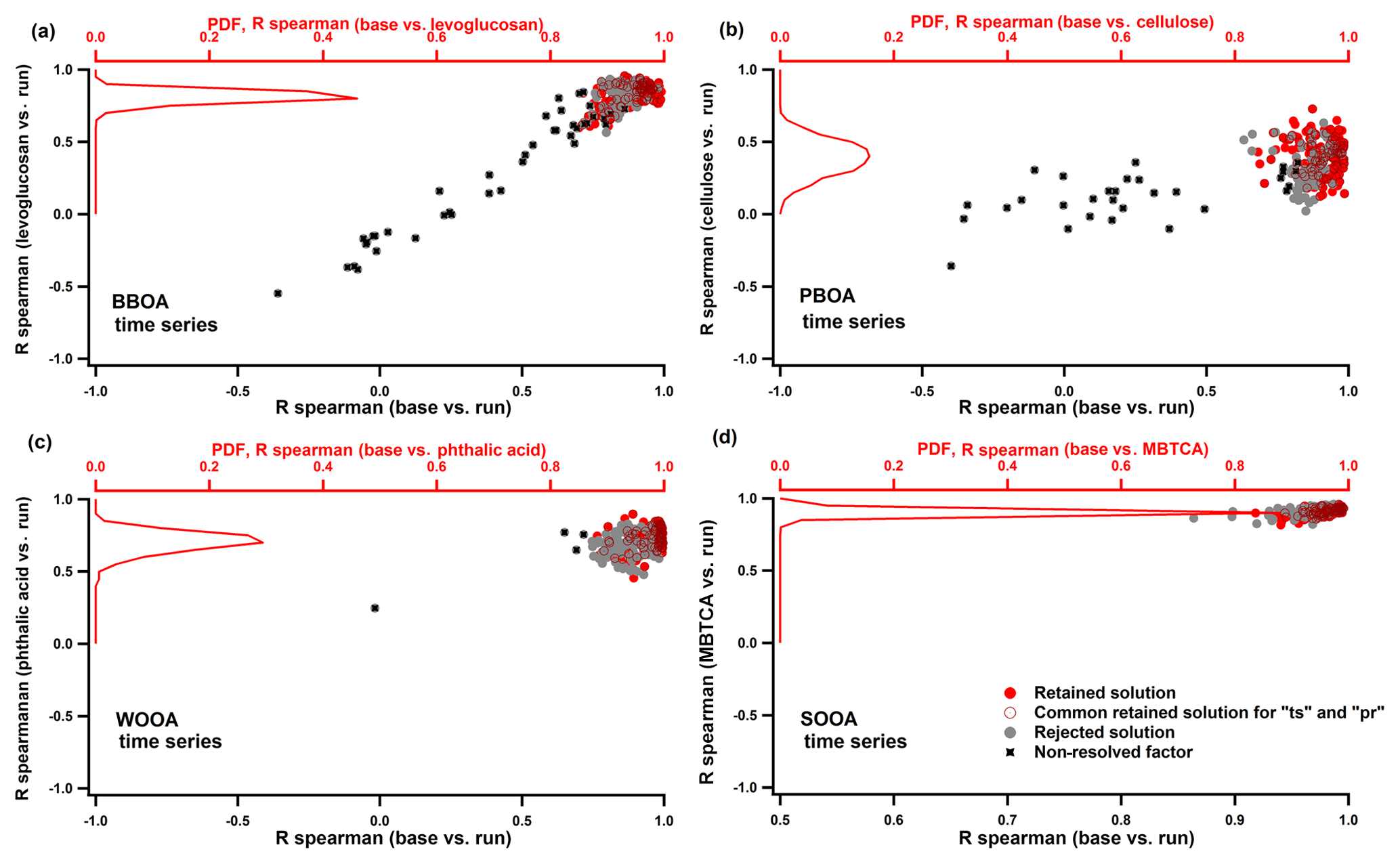
Figure 3Solution space per factor, defined by investigation of the correlation (Rs) between base-case time series and bootstrap runs (bottom x axis) and external markers and bootstrap runs (y axis): BBOA with levoglucosan (a), PBOA with cellulose (b), WOOA with phthalic acid (c) and SOOA with MBTCA (d). The retained solutions are indicated in red, and the rejected ones are indicated in grey. The points in black represent the runs where the specific factor was not resolved at all. Each PDF (top x axis) includes the range of R coming from the correlations between the time series of the base-case factors with their respective markers.
To assess whether the retained bootstrap solutions share the same quality with the base-case solution with regard to correlations between factors and markers, we calculated the probability of type I (false positive) and type II (false negative) errors associated with the solution selection approach (Fig. 4). The analysis entailed a quantitative comparison of the Spearman coefficients obtained between markers and factor time series from the bootstrap iterations, , with the respective Spearman coefficients obtained between markers and factor time series from the base case , considering the same samples as in the corresponding bootstrap iterations. The comparison between and was performed by applying a Fisher transformation followed by a t test. We defined true positive and false negative as the red (retained solutions) and black (non-resolved factors) points, respectively, lying within the PDF boundaries with regard to the total number of red and black points within the PDF boundaries. True negative and false positive were defined as the black and red points lying outside the PDF boundaries with respect to the total number of red and black points outside the PDF boundaries. The limits between false positive and false negative were set by 2 standard deviations from the one-to-one line. The percentages of the accuracy and the probability of false positive or false negative cases are compiled in Table S3. Sorting based on profiles seemed less reliable and is more prone to false negative solutions (Tables S3 and S4), as the profiles often look similar, and therefore the Rs exhibits high values for all factors (Fig. 2b and d). On the contrary, sorting based on time series showed clearer results, as the Rs spanned over a greater range of values (Fig. 2a and c). Still the ts method produced false negative solutions, for example 53 % for PBOA due to the combination of (i) a limited number of points available for cellulose and (ii) the representativeness of the marker time series after the resampling (bootstrap analysis). Note that PBOA was important only during a few days in spring, and therefore it is possible that these days were not always selected in the resampling process. The SOOA on the other hand exhibited 0 % false negative and 16 % false positive cases, always demonstrating high and values.
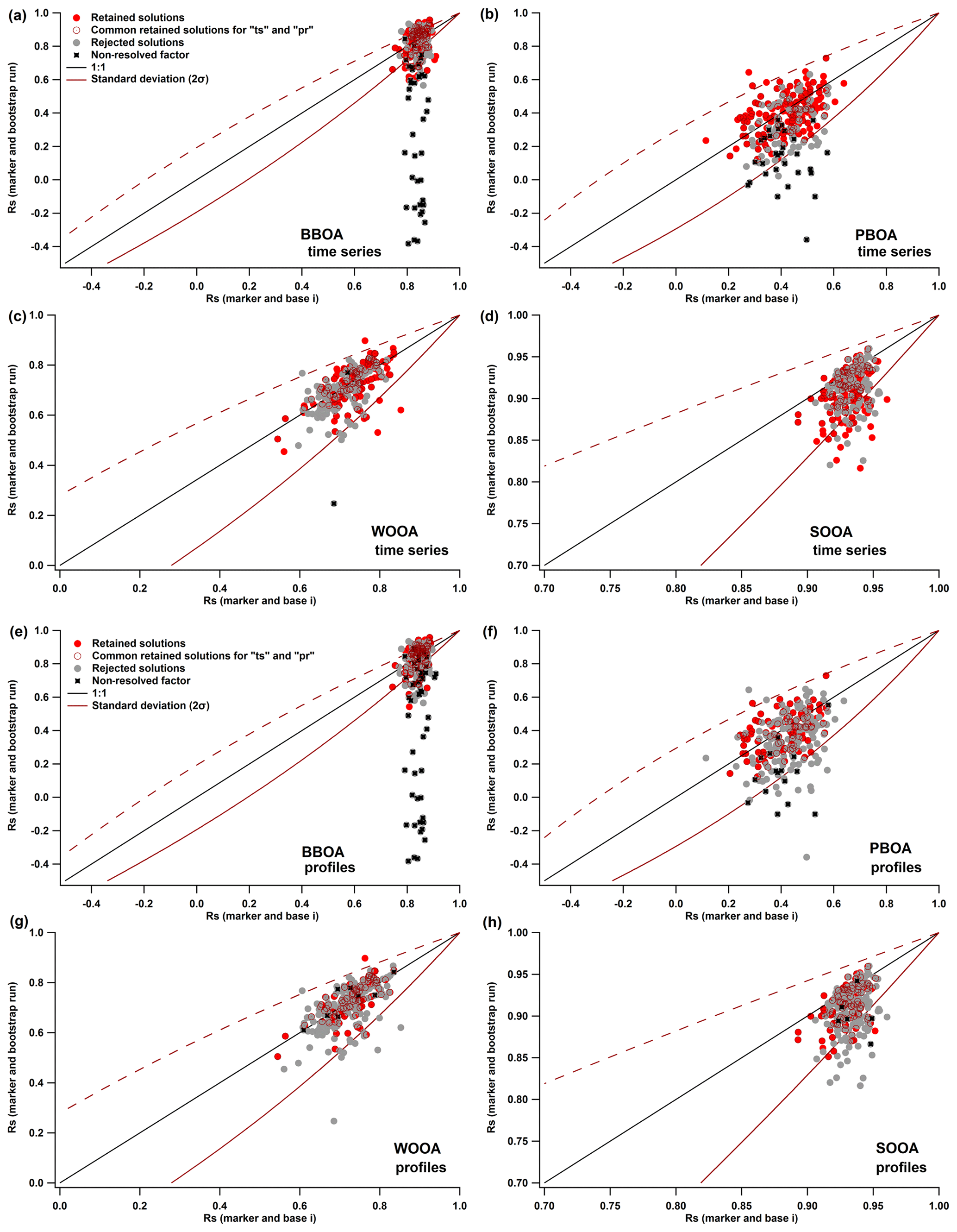
Figure 4Scatterplots of between markers and bootstrap runs and between markers and base cases per factor: BBOA with levoglucosan (a), PBOA with cellulose (b), WOOA with phthalic acid (c) and SOOA with MBTCA (d) for the ts sorting method. The black points that lie below the 1σ line (in solid dark red) indicate true negative solutions, whereas the black points within 2σ indicate false negative solutions. The red points below 1σ represent the false positive solutions, while the red points above are the true positive solutions. The respective scatterplots for the pr method are shown in (e), (f), (g) and (h). Note the different Rs scales per factor.
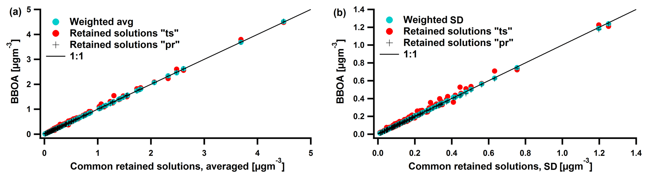
Figure 5(a) Scatterplots between BBOA time series averaged (avg) over the common solutions coming from both the time series (ts) and profile (pr) sorting method plotted in the x axis, and plotted in the y axis the BBOA time series averaged over the solutions coming from the ts method in red, from the pr in black cross and from the weighted average based on the marker (here levoglucosan, in blue). The respective scatterplot for the standard deviation (SD) is shown in (b).
However, in either of the two methods ts and pr, the Fisher-transformed correlation coefficient rendered the selection of the solution evident, and eventually the two sorting methods yielded a very similar retained solution space (Figs. 4 and 5). Figure 5 depicts the correlation between the averaged common retained solutions and the averaged retained solutions coming from either the ts or the pr sorting method for the example of BBOA (correlations for the other factors are shown in Fig. S3). There is a minor deviation from the one-to-one line for the standard deviation scatterplot (Fig. 5b) for the ts sorting method. However, as soon as the solutions were weighted according to the correlation between external marker and bootstrap run time series, then the deviation decreased (blue markers in Fig. 5). The weighting factor wi was calculated as
where SE is the standard error resulting from the regression between the external marker and bootstrap iteration.
4.1 Estimation of traffic contribution to EC and OC
We estimated above that the traffic contribution to WSOA (< 1 %) can be neglected and has little effect on the PMF outputs. However, traffic might be an important source of EC and OA, which is assessed in the following.
To estimate the percentage of EC coming from traffic (ECtr), we used the ME-2 model (with SoFi standard version 6.399; Canonaco et al., 2013), assuming that the sources of EC are biomass burning, resuspension of road dust, industrial emissions from the oil shale factories and traffic. Here the input data matrix included the time series of water-soluble biomass burning OA (WSBBOA), water-soluble sulfur-containing OA (WSSCOA), water-soluble oil OA (WSOilOA) and EC. PMF was conducted 1000 times, varying the initial seed to solve Eq. (4):
Here, ECbb, ECoil and ECrrd represent the EC concentration time series related to the primary sources biomass burning, oil shale industry, and resuspension of road dust and tire wear, respectively, while a, b and c are the EC : WSOA ratios characteristic of the emissions from the same sources and were obtained as outputs of the model. This new methodology, based on PMF, is especially pertinent, as unlike other inversion techniques, it sets positive constraints on a, b and c and offers the possibility of resolving the contributions of factors for which no constraints are available, here ECtr.
We found that ECtr contributed 57 % ± 5 % to the total EC (on a yearly average), while 36 % ± 5 % of EC was attributed to biomass burning, 4 % ± 1 % to road dust resuspension and 3 % ± 1 % to the oil shale emissions (Fig. S4). The contribution of EC from fossil fuel combustion (ECff) measured at a site similar to Tartu, i.e., an Alpine valley in Magadino, southern Switzerland, in 2014 (Vlachou et al., 2018), was in agreement with our ECtr contribution, with a yearly average of 55 % ± 7 %. Also, in Zurich, an urban site, ECff ranged from 40 % to 55 % during the winter of 2012 (Zotter et al., 2014). From the ECtr contribution, we estimated that the HOC (obtained by multiplication of the ECtr time series with the HOC:EC ratio) contributed 4 % to the total OC on a yearly average.
4.2 Scaling to organic carbon
All the retained solutions (in total 62 %) were averaged per factor, and their seasonal behavior as well as their correlations, with the external markers, are presented in Sect. 4.4. Note that all the water-soluble factors were recovered following the method described in Daellenbach et al. (2016) and Vlachou et al. (2018). The recoveries were calculated by fitting Eq. (5):
where OCi,n is the OC concentration per bootstrap run n per sample i, Rk is the recovery R per factor k, and is the water-soluble OC concentration calculated based on the measured WSOC and the OM:OC per factor. From the OCi,n the part of hydrocarbon-like OC and the inorganic carbon related to dust were removed. The carbonate-carbon investigation and calculation is discussed in Sect. 4.3. To define the recoveries, we used a non-negative multilinear fit. The starting points of the fitting for each Rk with the exception of Roil were obtained from the literature (Bozzetti et al., 2016; Daellenbach et al. 2016; Vlachou et al., 2018) and were randomly varied within their literature range with an increment of 10−4. The final distributions of the recoveries are shown in the Supplement (Fig. S5). The recoveries in this study were all shifted to the lower end of the recoveries reported in the literature. While the reason remains unclear, the water solubility of OA is specific to the dataset; therefore we can expect differences to other datasets. Moreover, we re-measured, in a different laboratory, the OC concentrations from a subset of 21 samples covering all sites and all seasons. The agreement between the two differently determined OC concentrations was excellent (Fig. S6; slope = 0.93, R2=0.99).
4.3 Exploration of the dust factor
Mineral dust can contain a significant amount of inorganic carbon in the form of . The water extracts used in the offline AMS technique have a pH that is always < 8. Therefore, the in our samples is all solubilized into (pKa () = 10.33; Bruice, 2010). This is shown to release CO2 when it undergoes thermal decomposition on the AMS vaporizer (at 600 ∘C; Bozzetti et al., 2017b). Thus, the contribution of to organic aerosols is overestimated and the fraction coming from the inorganic carbon should be removed from the OA spectra.
To remove the influence of the inorganic dust, we estimated the carbonate-carbon concentrations [C_CO3] corrected for the relative ionization efficiency, as discussed in the Supplement. This estimated C_CO3 concentration was compared to measured carbonate on a subset of 19 filter samples. While the agreement between measured and estimated concentrations is poor for Tartu, a decent agreement was found for KJ and Tallinn, especially given the large uncertainties in both variables (Fig. S7). On an absolute basis, PMF seems to overestimate the C_CO3 concentrations by ∼20 % compared to the measured concentrations.
Ca2+ is one of the most common constituents of mineral dust and can therefore be used to trace this source. The time series of C_CO3 and Ca2+, available for the entire set of samples, displayed in Fig. 6, show that the two variables exhibit similar trends (except for Tallinn). Despite the large errors in the [C_CO3] estimates, an uncertainty weighted correlation analysis (Supplement and Fig. S8) shows that [C_CO3] and [Ca2+] correlate statistically significantly (R=0.4, p < 10−5) with a slope of 0.2, consistent with C_CO3 and Ca2+ being in the form of calcium bicarbonate.
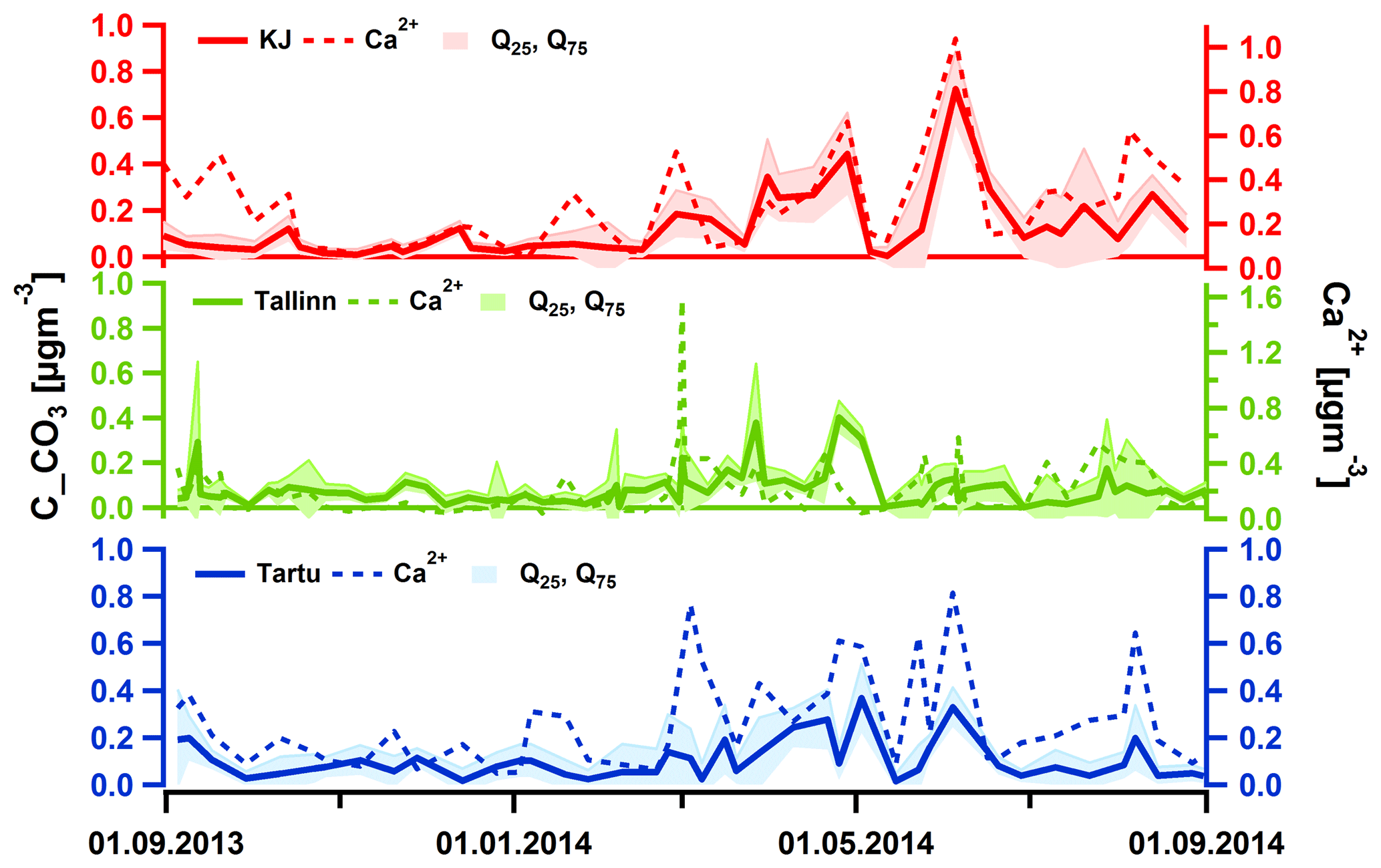
Figure 6Time series of the inorganic dust factor [C_CO3] with interquartile ranges (Q25 and Q75) and of Ca2+ per site.
We have validated the identity of the dust factor even further by measuring the same subset of 19 filters with the offline AMS technique before and after fumigation with HCl (as described in Zhang et al., 2016). The comparison of the mass spectra of fumigated and non-fumigated samples is illustrated in Fig. 7 for two samples: with high and low contribution of dust. In the example of KJ (5 June 2014), where the dust factor exhibited the highest contribution, f44 was substantially decreased after fumigation (Fig. 7a). In the case of Tallinn (19 January 2014), where the dust factor concentration was negligible, f44 remained stable after fumigation (Fig. 7b). Overall, the comparison of the Δf44 modeled (=f44total–f44org) from the initial dataset of 150 filters and the Δf44 measured (=f44non_fum–f44fum) from the subset of 19 filters showed consistent results (Fig. 8). Taken together these results provide strong confidence on the nature of the dust factor extracted by PMF.

Figure 7Example mass spectra from two fumigated and non-fumigated samples, with a high (KJ on 5 June 2014; a), and a low dust concentration (Tallinn on 19 January 2014; b).

4.4 Seasonal variation of organic aerosol sources
The sources were quantified after removing the contribution of the dust factor from the total OA. All the factor concentrations with their uncertainties averaged per season are presented in Table S3. In general, the relative uncertainties decreased with increasing concentrations per factor (Fig. S9). For concentrations above ∼1 µg m−3 the percentage error became more important than the error related to noise and was thus more stable for all factors. Consistent with the factor separation and uncertainty analysis above, the factors that were well separated, such as SOOA, exhibited low relative uncertainty (0.15), while the factors that were more difficult to extract, such as BBOA, exhibited higher relative uncertainty (0.45).
BBOA exhibited high concentrations in Tallinn during winter (on average 3.7±2.7 µg m−3) and fall (1.2 ± 0.9 µg m−3) and in Tartu (8.4 ± 3.9 and 3.8 ± 1.9 µg m−3, winter and fall, respectively; Fig. 9a; Table S5). In both cities BBOA and the marker levoglucosan correlated very well (Fig. 9b) confirming the identity of the factor. For KJ the concentrations of BBOA were lower in winter (1.3±0.8 µg m−3) as expected, due to the low number of residents and low biomass burning activities in the region. At all sites the levoglucosan-to-BBOA ratio (0.08 for KJ, 0.05 for Tallinn and 0.05 for Tartu) assessed in this study was consistent with the one reported in the neighboring country, Lithuania (Bozzetti et al., 2017a). Potassium (K+), which is often used as a wood-burning marker, especially for ash, also correlated well with BBOA for Tallinn (R2=0.80) and Tartu (R2=0.58). Different ratios were used in the past to describe burning conditions (Zotter et al., 2014; Daellenbach et al., 2018), and higher values were linked to inefficient burning conditions. Here, the ratio (14.3 for Tallinn and 18.1 for Tartu) was in agreement with the one found at southern Alpine valley sites (Magadino and San Vittore, Switzerland; Daellenbach et al., 2018) where older stoves are still used. In Estonia more than 80 % of households use old types of stoves for heating purposes (Maasikmets et al., 2015); therefore, BBOA could be linked to inefficient residential wood burning.
The recognition of PBOA as described in Sect. 3.2 was also supported by the high correlations of this factor with cellulose and erythritol (Fig. 9d). Cellulose is related to plant debris and is typically used as a marker for primary biological aerosols (Bozzetti et al., 2016), while erythritol, among other sugar alcohols, reflects airborne biogenic detritus (Graham et al., 2002). The seasonal behavior of PBOA was very similar to the respective behavior of both markers (Fig. 9c), with average spring concentrations of 0.2 ± 0.2 µg m−3 for KJ, 1.2 ± 0.8 µg m−3 for Tallinn and 0.7 ± 0.4 µg m−3 for Tartu.
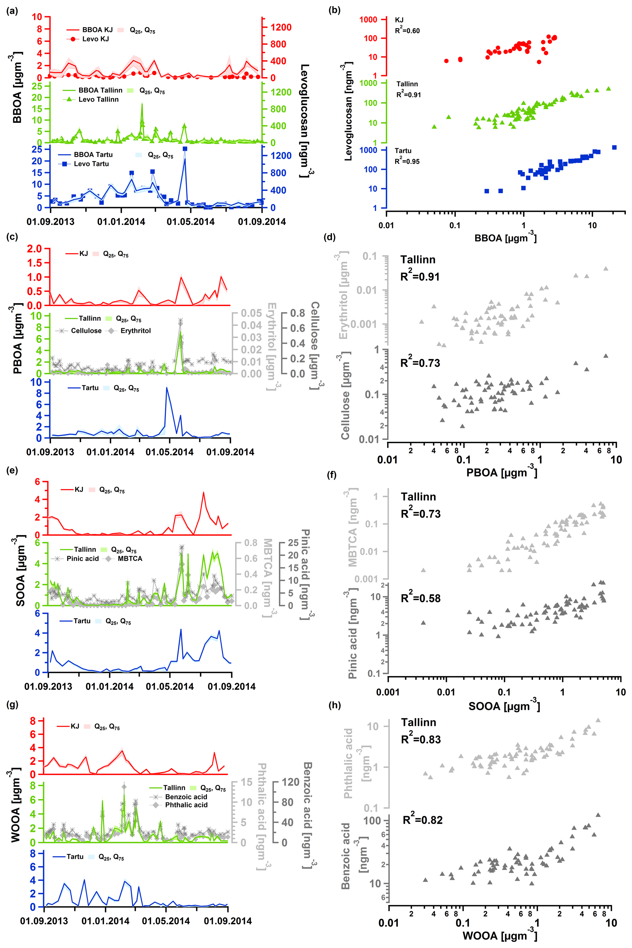
Figure 9Factor median and external marker concentration time series for all three sites: (a) BOOA and levoglucosan (note the change of the scale for KJ); (c) PBOA, cellulose and erythritol (note the change of the scale for KJ); (e) SOOA, pinic acid and MBTCA; and (g) WOOA, benzoic and phthalic acid, with the respective scatterplots between factors and external markers in (b), (d), (f) and (h). The colors red, green and blue denote the site (KJ, Tallinn and Tartu), and the markers in light and dark grey denote the concentrations of the external markers. The shaded areas represent the first (Q25) and third (Q75) quartiles.
SOOA exhibited a clear yearly cycle at all sites, with the highest concentrations witnessed in summer and early fall (in summer on average 1.8 ± 0.7 µg m−3 for KJ, 2.8 ± 0.6 µg m−3 for Tallinn and 2.1 ± 0.4 µg m−3 for Tartu; Fig. 9e). In previous studies this factor showed an exponential increase (Fig. S10) with temperature and was linked to terpene oxidation products (Daellenbach et al., 2017; Leaitch et al., 2011). In another study in an Alpine valley site, this factor was also found to be 79 % non-fossil, supporting the connection to biogenic secondary OA (Vlachou et al., 2018). Here, SOOA not only correlated with temperature (Rs=0.77; Fig. S10) but also with two oxidation products of a-pinene, i.e., with pinic acid and even better with MBTCA (Fig. 9f). The latter was shown to be produced by reaction of pinonic acid with the OH radical (Müller et al., 2012).
WOOA was more pronounced during fall and winter at all sites, with average concentrations in winter of 1.4 ± 0.5 µg m−3 for KJ, 2.2±0.8 µg m−3 for Tallinn, and 1.5 ± 0.5 µg m−3 for Tartu (Fig. 9g). In earlier studies WOOA was characterized as non-fossil (Vlachou et al., 2018) and was identified based on its correlation with coming mainly from NH4NO3 in the wintertime (Lanz et al., 2007; Daellenbach et al., 2017). It was also related to long-range transported oxygenated OA stemming from anthropogenic emissions during winter, such as biomass burning. Also, WOOA demonstrated high correlations with two anthropogenic organic acids, benzoic and phthalic acid (Fig. 9h), formed via the photo-oxidation of aromatic hydrocarbons such as toluene and naphthalene and therefore suggested to be tracers for anthropogenic sources (Kawamura and Yasui, 2005; Deshmukh et al., 2016). Recently, Bruns et al. (2016) found that aromatic compounds, such as benzene and naphthalene emitted by wood combustion, can indeed produce highly oxygenated SOA. Taking all the above into account, it was concluded that WOOA might be linked mostly to aged wood-burning OA.
Figure 10 illustrates the relative contributions per factor per site to the total OA (all averaged contributions per season per factor with their uncertainties shown in Table S6). Out of the primary sources, the major contributor was BBOA during winter and fall (on average and 1 standard deviation: 39 % ± 16 % and 27 % ± 13 % in Tallinn and 73 % ± 21 % and 53 % ± 14 % in Tartu). However, in KJ during winter and fall, WOOA was the dominant source (36 % ± 14 % and 39 % ± 13 %, respectively), indicating that for this site, regional transport of OA is important. In spring, PBOA was the major source in Tartu (21 % ± 8 %), while in Tallinn BBOA and SOOA were the dominating sources during that season (30 % ± 14 % and 18 % ± 5 %, respectively). This could be due to the fact that temperatures in early spring are still low (2 ∘C on average in Tallinn in March) and the wood burning for residential heating is still widely used. Towards the end of spring (15 ∘C on average in Tallinn in May) the rising temperature favors the biogenic emissions. In KJ, the most important source was oil OA (36 % ± 14 % in spring), most possibly coming from the oil shale industries in the region. The presence of the oil factor at the other two sites could be an indication that this factor is mixed with coal or waste burning, as also found by Elser et al. (2016). Besides this, the oil OA profile resembled the coal profile identified in the city of Cork, Ireland (Dall'Osto et al., 2013). During the summer months and early fall, SOOA prevailed over all sources at all sites, with 26 % ± 5 % in KJ, 41 % ± 7 % in Tallinn and 35 % ± 7 % in Tartu. Even though KJ is highly industrialized, SOOA can still be related to the production of secondary OA from biogenic volatile organic compounds. The least-significant source, especially in Tartu, with rather stable seasonal behavior, was SCOA. The yearly average contribution of SCOA was 12 % ± 4 % in KJ, 14 % ± 5 % in Tallinn and 4 % ± 2 % in Tartu. Although it is generally found that the secondary sources prevail over the primary ones, here the primary sources seem to dominate the secondary ones. This is also observed at other European sites such as Payerne (Bozzetti et al., 2016, for coarse particles) or Magadino, especially in winter (Vlachou et al., 2018, for PM10), as well as in Beijing, China (Zhang et al., 2017, for PM1).
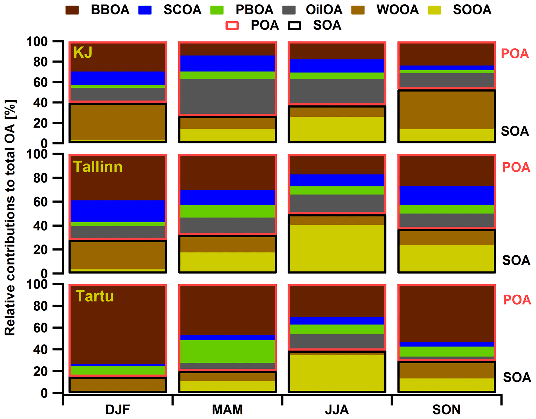
Figure 10Seasonally averaged relative contributions of each factor to the total OA per site. The red and black boxes indicate the contributions of primary and secondary OA, respectively.
The offline AMS technique was applied to a set of 150 filter samples covering a yearly cycle at three sites in Estonia. The uncertainties of the PMF solution were assessed by bootstrap analysis. In order to identify the factors, the Spearman R (Rs) coefficients between base-case time series and bootstrap run time series (ts) as well as base-case profiles and bootstrap run profiles (pr) were monitored. The results showed that the retained solution space if one follows the ts or the pr sorting method is very similar. Weighting with the Rs between external markers and bootstrap run increased our confidence towards the solution space. The source apportionment results revealed four primary OA sources, two secondary OA and a dust factor. The dust factor was identified by measurements of calcium carbonate as well as by acidification with HCl of a selected batch of filters. Out of the primary sources, three had an anthropogenic influence. BBOA was mainly present in winter and autumn in Tallinn and Tartu, the two largest cities of Estonia, where residential heating activities are common. SCOA was mostly important in winter in Tallinn and KJ, in contrast to Tartu. The third anthropogenic primary factor was oil OA, which exhibited the highest concentrations in KJ, as expected. The reason why this factor was evident in Tallinn and Tartu could be that it may include coal combustion for residential heating purposes. PBOA was the only primary OA not related to anthropogenic emissions and prevailed in spring at all sites. The two oxygenated OA factors were separated according to their seasonal behavior: WOOA was linked to anthropogenic wood-burning activities, as it dominated in winter and autumn at all sites and also correlated with phthalic and benzoic acid. SOOA was significant during summer at all sites and was related to biogenic emissions and strong aging, as it was highly correlated with a second-generation oxidation product of a-pinene.
The data of each figure are available here: https://doi.org/10.5281/zenodo.3218429 (Vlachou et al., 2019).
The supplement related to this article is available online at: https://doi.org/10.5194/acp-19-7279-2019-supplement.
AV performed the offline AMS measurements, data curation and formal analysis; AV and IEH wrote the paper; AT assisted with the formal analysis; HL provided expertise on AMS measurements; FC and KD provided expertise on software; JLJ performed additional measurements including major ions, sugars, organic acids, cellulose, OC–EC and WSOC; MCM performed the carbonate measurements; MM and ET organized the filter sampling; and UB, ASHP and IEH were involved with the supervision and conceptualization. All authors commented on the paper and assisted in the interpretation of the results.
The authors declare that they have no conflict of interest.
This work was funded by the Estonian–Swiss cooperation program “Enforcement of the surveillance network of the Estonian air quality: Determination of origin of fine particles in Estonia”. María Cruz Minguillón acknowledges the Ramón y Cajal Fellowship awarded by the Spanish Ministry of Economy, Industry and Competitiveness. The Labex OSUG@2020 (ANR-10-LABX-56) provided the funding for part of the analytical equipment at Institut des Géosciences de l'Environnement (IGE; France). We also acknowledge the contribution of the COST Action CA16109 COLOSSAL.
This paper was edited by James Allan and reviewed by two anonymous referees.
Alfarra, M. R., Prevot, A. H. S., Szidat, S., Sandradewi, J., Weimer, S., Lanz, V. A., Schreiber, D., Mohr, M., and Baltensperger, U.: Identification of the mass spectral signature of organic aerosols from wood burning emissions, Environ. Sci. Technol., 41, 5770–5777, https://doi.org/10.1021/es062289b, 2007.
Birch, M. E. and Cary, R. A.: Elemental carbon-based method for monitoring occupational exposures to particulate diesel exhaust, Aerosol Sci. Tech., 25, 221–241, 1996.
Bozzetti, C., Daellenbach, K. R., Hueglin, C., Fermo, P., Sciare, J., Kasper-Giebl, A., Mazar, Y., Abbaszade, G., El Kazzi, M., Gonzalez, R., Shuster Meiseles, T., Flasch, M., Wolf, R., Křepelová, A., Canonaco, F., Schnelle-Kreis, J., Slowik, J. G., Zimmermann, R., Rudich, Y., Baltensperger, U., El Haddad, I., and Prévôt, A. S. H.: Size-resolved identification, characterization, and quantification of primary biological organic aerosol at a European rural site, Environ. Sci. Technol., 50, 3425–3434, https://doi.org/10.1021/acs.est.5b05960, 2016.
Bozzetti, C., Sosedova, Y., Xiao, M., Daellenbach, K. R., Ulevicius, V., Dudoitis, V., Mordas, G., Bycenkiene, S., Plauškaite, K., Vlachou, A., Golly, B., Chazeau, B., Besombes, J.-L., Baltensperger, U., Jaffrezo, J.-L., Slowik, J. G., El Haddad, I., and Prévôt, A. S. H.: Argon offline-AMS source apportionment of organic aerosol over yearly cycles for an urban, rural, and marine site in northern Europe, Atmos. Chem. Phys., 17, 117–141, https://doi.org/10.5194/acp-17-117-2017, 2017a.
Bozzetti, C., El Haddad, I., Salameh, D., Daellenbach, K. R., Fermo, P., Gonzalez, R., Minguillón, M. C., Iinuma, Y., Poulain, L., Elser, M., Müller, E., Slowik, J. G., Jaffrezo, J.-L., Baltensperger, U., Marchand, N., and Prévôt, A. S. H.: Organic aerosol source apportionment by offline-AMS over a full year in Marseille, Atmos. Chem. Phys., 17, 8247–8268, https://doi.org/10.5194/acp-17-8247-2017, 2017b.
Brown, S. G., Eberly, S., Norris, G. A., and Paatero, P.: Methods for estimating uncertainty in PMF solutions: examples with ambient air and water quality data and guidance on reporting PMF results, Sci. Total Environ., 518–519, 626–635, https://doi.org/10.1016/j.scitotenv.2015.01.022, 2015.
Bruice, P. Y.: Organic chemistry, Prentice Hall, New Jersey, 2010.
Bruns, E. A., El Haddad, I., Slowik, J. G., Kilic, D., Klein, F., Baltensperger, U., and Prévôt, A. S. H.: Identification of significant precursor gases of secondary organic aerosols from residential wood combustion, Sci. Rep., 6, 27881, https://doi.org/10.1038/srep27881, 2016.
Canagaratna, M. R., Jayne, J. T., Jimenez, J. L., Allan, J. D., Alfarra, M. R., Zhang, Q., Onasch, T. B., Drewnick, F., Coe, H., Middlebrook, A., Delia, A., Williams, L. R., Trimborn, A. M., Northway, M. J., DeCarlo, P. F., Kolb, C. E., Davidovits, P., and Worsnop, D. R.: Chemical and microphysical characterization of ambient aerosols with the Aerodyne aerosol mass spectrometer, Mass Spectrom. Rev., 26, 185–222, https://doi.org/10.1002/mas.20115, 2007.
Canonaco, F., Crippa, M., Slowik, J. G., Baltensperger, U., and Prévôt, A. S. H.: SoFi, an IGOR-based interface for the efficient use of the generalized multilinear engine (ME-2) for the source apportionment: ME-2 application to aerosol mass spectrometer data, Atmos. Meas. Tech., 6, 3649–3661, https://doi.org/10.5194/amt-6-3649-2013, 2013.
Canonaco, F., Slowik, J. G., Baltensperger, U., and Prévôt, A. S. H.: Seasonal differences in oxygenated organic aerosol composition: implications for emissions sources and factor analysis, Atmos. Chem. Phys., 15, 6993–7002, https://doi.org/10.5194/acp-15-6993-2015, 2015.
Cavalli, F., Viana, M., Yttri, K. E., Genberg, J., and Putaud, J.-P.: Toward a standardised thermal-optical protocol for measuring atmospheric organic and elemental carbon: the EUSAAR protocol, Atmos. Meas. Tech., 3, 79–89, https://doi.org/10.5194/amt-3-79-2010, 2010.
Crippa, M., DeCarlo, P. F., Slowik, J. G., Mohr, C., Heringa, M. F., Chirico, R., Poulain, L., Freutel, F., Sciare, J., Cozic, J., Di Marco, C. F., Elsasser, M., Nicolas, J. B., Marchand, N., Abidi, E., Wiedensohler, A., Drewnick, F., Schneider, J., Borrmann, S., Nemitz, E., Zimmermann, R., Jaffrezo, J.-L., Prévôt, A. S. H., and Baltensperger, U.: Wintertime aerosol chemical composition and source apportionment of the organic fraction in the metropolitan area of Paris, Atmos. Chem. Phys., 13, 961–981, https://doi.org/10.5194/acp-13-961-2013, 2013.
Daellenbach, K. R., Bozzetti, C., Krepelová, A., Canonaco, F., Wolf, R., Zotter, P., Fermo, P., Crippa, M., Slowik, J. G., Sosedova, Y., Zhang, Y., Huang, R.-J., Poulain, L., Szidat, S., Baltensperger, U., El Haddad, I., and Prévôt, A. S. H.: Characterization and source apportionment of organic aerosol using offline aerosol mass spectrometry, Atmos. Meas. Tech., 9, 23–39, https://doi.org/10.5194/amt-9-23-2016, 2016.
Daellenbach, K. R., Stefenelli, G., Bozzetti, C., Vlachou, A., Fermo, P., Gonzalez, R., Piazzalunga, A., Colombi, C., Canonaco, F., Hueglin, C., Kasper-Giebl, A., Jaffrezo, J.-L., Bianchi, F., Slowik, J. G., Baltensperger, U., El-Haddad, I., and Prévôt, A. S. H.: Long-term chemical analysis and organic aerosol source apportionment at nine sites in central Europe: source identification and uncertainty assessment, Atmos. Chem. Phys., 17, 13265–13282, https://doi.org/10.5194/acp-17-13265-2017, 2017.
Daellenbach, K. R., El-Haddad, I., Karvonen, L., Vlachou, A., Corbin, J. C., Slowik, J. G., Heringa, M. F., Bruns, E. A., Luedin, S. M., Jaffrezo, J.-L., Szidat, S., Piazzalunga, A., Gonzalez, R., Fermo, P., Pflueger, V., Vogel, G., Baltensperger, U., and Prévôt, A. S. H.: Insights into organic-aerosol sources via a novel laser-desorption/ionization mass spectrometry technique applied to one year of PM10 samples from nine sites in central Europe, Atmos. Chem. Phys., 18, 2155–2174, https://doi.org/10.5194/acp-18-2155-2018, 2018.
Dall'Osto, M., Ovadnevaite, J., Ceburnis, D., Martin, D., Healy, R. M., O'Connor, I. P., Kourtchev, I., Sodeau, J. R., Wenger, J. C., and O'Dowd, C.: Characterization of urban aerosol in Cork city (Ireland) using aerosol mass spectrometry, Atmos. Chem. Phys., 13, 4997–5015, https://doi.org/10.5194/acp-13-4997-2013, 2013.
Davison, A. C. and Hinkley, D. V.: Bootstrap Methods and Their Application, Cambridge University Press, Cambridge, UK, 582 pp., 1997.
Deshmukh, D. K., Kawamura, K., Lazaar, M., Kunwar, B., and Boreddy, S. K. R.: Dicarboxylic acids, oxoacids, benzoic acid, a-dicarbonyls, WSOC, OC, and ions in spring aerosols from Okinawa Island in the western North Pacific Rim: size distributions and formation processes, Atmos. Chem. Phys., 16, 5263–5282, https://doi.org/10.5194/acp-16-5263-2016, 2016.
Elser, M., Bozzetti, C., El-Haddad, I., Maasikmets, M., Teinemaa, E., Richter, R., Wolf, R., Slowik, J. G., Baltensperger, U., and Prévôt, A. S. H.: Urban increments of gaseous and aerosol pollutants and their sources using mobile aerosol mass spectrometry measurements, Atmos. Chem. Phys., 16, 7117–7134, https://doi.org/10.5194/acp-16-7117-2016, 2016.
Elser, M., El-Haddad, I., Maasikmets, M., Bozzetti, C., Wolf, R., Ciarelli, G., Slowik, J. G., Richter, R., Teinemaa, E., Hüglin, C., Baltensperger, U., and Prévôt, A. S. H.: High contributions of vehicular emissions to ammonia in three European cities derived from mobile measurements, Atmos. Environ., 175, 210–220, https://doi.org/10.1016/j.atmosenv.2017.11.030, 2018.
El Haddad, I., D'Anna, B., Temime-Roussel, B., Nicolas, M., Boreave, A., Favez, O., Voisin, D., Sciare, J., George, C., Jaffrezo, J.-L., Wortham, H., and Marchand, N.: Towards a better understanding of the origins, chemical composition and aging of oxygenated organic aerosols: case study of a Mediterranean industrialized environment, Marseille, Atmos. Chem. Phys., 13, 7875–7894, https://doi.org/10.5194/acp-13-7875-2013, 2013.
European Environment Agency: report No 13/2017: Air quality in Europe 2017.
Fuzzi, S., Baltensperger, U., Carslaw, K., Decesari, S., Denier van der Gon, H., Facchini, M. C., Fowler, D., Koren, I., Langford, B., Lohmann, U., Nemitz, E., Pandis, S., Riipinen, I., Rudich, Y., Schaap, M., Slowik, J. G., Spracklen, D. V., Vignati, E., Wild, M., Williams, M., and Gilardoni, S.: Particulate matter, air quality and climate: lessons learned and future needs, Atmos. Chem. Phys., 15, 8217–8299, https://doi.org/10.5194/acp-15-8217-2015, 2015.
Graham, B., Mayol-Bracero, O. L., Guyon P., Roberts, C. G., Decesari, S., Facchini, C. M., Artaxo, P., Maenhaut, W., Köll, P., and Andreae, M. O.: Water-soluble organic compounds in biomass burning aerosols over Amazonia 1, Characterization by NMR and GC-MS, J. Geophys. Res., 107, 8047, https://doi.org/10.1029/2001JD000336, 2002.
Henry, R. C.: Current factor analysis models are ill-posed, Atmos. Environ., 21, 1815–1820, https://doi.org/10.1016/0004-6981(87)90122-3, 1987.
Huang, R.-J., Zhang, Y., Bozzetti, C., Ho, K.-F., Cao, J., Han, Y., Dällenbach, K. R., Slowik, J. G., Platt, S. M., Canonaco, F., Zotter, P., Wolf, R., Pieber, S. M., Bruns, E. A., Crippa, M., Ciarelli, G., Piazzalunga, A., Schwikowski, M., Abbaszade, G., Schnelle-Kreis, J., Zimmermann, R., An, Z., Szidat, S., Baltensperger, U., Haddad, I. E., and Prévôt, A. S. H.: High secondary aerosol contribution to particulate pollution during haze events in China, Nature, 514, 218–222, https://doi.org/10.1038/nature13774, 2014.
Jacob, V., Golly, B., Gigneys, S., Donnaz, F., Masson, F., Besombes, J. -L., and Jaffrezo, J. -L.: Organic acids in PM measured by LC-MS: seasonal variations in rural sites in France, Atmos. Meas. Tech., in preparation, 2019.
Jaffrezo, J.-L., Calas, T., and Bouchet, M.: Carboxylic acids measurements with ionic chromatography, Atmos. Environ., 32, 2705–2708, https://doi.org/10.1016/S1352-2310(98)00026-0, 1998.
Karanasiou, A., Diapouli, E., Cavalli, F., Eleftheriadis, K., Viana, M., Alastuey, A., Querol, X., and Reche, C.: On the quantification of atmospheric carbonate carbon by thermal/optical analysis protocols, Atmos. Meas. Tech., 4, 2409–2419, https://doi.org/10.5194/amt-4-2409-2011, 2011.
Kawamura, K. and Yasui, O.: Diurnal changes in the distribution of dicarboxylic acids, ketocarboxylic acids and dicarbonyls in the urban Tokyo atmosphere, Atmos. Environ., 39, 1945–1960, https://doi.org/10.1016/j.atmosenv.2004.12.014, 2005.
Kiesewetter, G., Borken-Kleefeld, J., Schöpp, W., Heyes, C., Thunis, P., Bessagnet, B., Terrenoire, E., Fagerli, H., Nyiri, A., and Amann, M.: Modelling street level PM10 concentrations across Europe: source apportionment and possible futures, Atmos. Chem. Phys., 15, 1539–1553, https://doi.org/10.5194/acp-15-1539-2015, 2015.
Kunit, M. and Puxbaum, H.: Enzymatic determination of the cellulose content of atmospheric aerosols, Atmos. Environ., 30, 1233–1236, https://doi.org/10.1016/1352-2310(95)00429-7, 1996.
Lanz, V. A., Alfarra, M. R., Baltensperger, U., Buchmann, B., Hueglin, C., and Prévôt, A. S. H.: Source apportionment of submicron organic aerosols at an urban site by factor analytical modelling of aerosol mass spectra, Atmos. Chem. Phys., 7, 1503–1522, https://doi.org/10.5194/acp-7-1503-2007, 2007.
Leaitch, W. R., Macdonald, A. M., Brickell, P. C., Liggio, J., Sjostedt, S. J., Vlasenko, A., Bottenheim, J. W., Huang, L., Li, S.-M., Liu, P. S. K., Toom-Sauntry, D., Hayden, K. A., Sharma, S., Shantz, N. C.,Wiebe H. A., Zhang,W., Abbatt, J. P. D., Slowik, J. G., Chang, R., Y.-W., Russell, L. M., Schwartz, R. E., Takahama, S., Jayne, J. T., and Ng, N. L.: Temperature response of the submicron organic aerosol from temperate forests, Atmos. Environ., 45, 6696–6704, https://doi.org/10.1016/j.atmosenv.2011.08.047, 2011.
Maasikmets, M., Kupri, H.-L., Teinemaa, E., Vainumäe, K., Arumäe, T., and Kimmel, V.: ACSM study to assess possible municipal solid waste burning in household stoves, Poster presented at: European Aerosol Conference, Milan (Italy), 6–11 September, https://doi.org/10.13140/RG.2.1.2100.0167, 2015.
Mohr, C., DeCarlo, P. F., Heringa, M. F., Chirico, R., Slowik, J. G., Richter, R., Reche, C., Alastuey, A., Querol, X., Seco, R., Peñuelas, J., Jiménez, J. L., Crippa, M., Zimmermann, R., Baltensperger, U., and Prévôt, A. S. H.: Identification and quantification of organic aerosol from cooking and other sources in Barcelona using aerosol mass spectrometer data, Atmos. Chem. Phys., 12, 1649–1665, https://doi.org/10.5194/acp-12-1649-2012, 2012.
Müller, L., Reinnig, M.-C., Naumann, K. H., Saathoff, H., Mentel, T. F., Donahue, N. M., and Hoffmann, T.: Formation of 3-methyl-1,2,3-butanetricarboxylic acid via gas phase oxidation of pinonic acid – a mass spectrometric study of SOA aging, Atmos. Chem. Phys., 12, 1483–1496, https://doi.org/10.5194/acp-12-1483-2012, 2012.
Myers, L. and Sirois, M. J.: Spearman Correlation Coefficients, Differences between Encyclopedia of Statistical Sciences, 12, https://doi.org/10.1002/0471667196.ess5050.pub2, 2006.
Norris, G., Duvall, R., Brown, S., and Bai, S.: EPA Positive Matrix Factorization (PMF) 5.0 Fundamentals and User Guide, Prepared for the, U.S. Environmental Protection Agency Office of Research and Development, Washington, DC (EPA/600/R-14/108; April), 2014.
Orru, H., Maasikmets, M., Lai, T., Tamm, T., Kaasik, M., Kimmel, V., Orru, K., Merisalu, E., and Forsberg, B.: Health impacts of particulate matter in five major Estonian towns: main sources of exposure and local differences, Air Qual. Atmos. Health, 4, 247–258, https://doi.org/10.1007/s11869-010-0075-6, 2010.
Paatero, P.: Least squares formulation of robust non-negative factor analysis, Chemom. Intell. Lab. Syst., 37, 23–35, https://doi.org/10.1016/S0169-7439(96)00044-5, 1997.
Paatero, P.: The multilinear engine – A table-driven, least squares program for solving multilinear problems, including the n-way parallel factor analysis model, J. Comput. Graph. Stat., 8, 854–888, 1999.
Paatero, P. and Hopke, P. K.: Rotational tools for factor analytic models, J. Chemometr., 23, 91–100, https://doi.org/10.1002/cem.1197, 2009.
Pieber, S. M., El Haddad, I., Slowik, J. G., Canagaratna, M. R., Jayne, J. T., Platt, S. M., Bozzetti, C., Daellenbach, K. R., Fröhlich, R., Vlachou, A., Klein, F., Dommen, J., Miljevic, B., Jimenez, J. L., Worsnop, D. R., Baltensperger, U., and Prévôt, A. S. H.: Inorganic salt interference on in aerodyne AMS and ACSM organic aerosol composition studies, Environ. Sci. Technol., 50, 10494–10503, https://doi.org/10.1021/acs.est.6b01035, 2016.
Piot, C., Jaffrezo, J.-L., Cozic, J., Pissot, N., El Haddad, I., Marchand, N., and Besombes, J.-L.: Quantification of levoglucosan and its isomers by High Performance Liquid Chromatography – Electrospray Ionization tandem Mass Spectrometry and its applications to atmospheric and soil samples, Atmos. Meas. Tech., 5, 141–148, https://doi.org/10.5194/amt-5-141-2012, 2012.
Putaud, J. P., Van Dingenen, R., Alastuey, A., Bauer, H., Birmili, W., Cyrys, J., Flentje, H., Fuzzi, S., Gehrig, R., Hansson, H. C., Harrison, R. M., Herrmann, H., Hitzenberger, R., Hüglin, C., Jones, A. M., Kasper-Giebl, A., Kiss, G., Kousa, A., Kuhlbusch, T. A. J., Löschau, G., Maenhaut, W., Molnar, A., Moreno, T., Pekkanen, J., Perrino, C., Pitz, M., Puxbaum, H., Querol, X., Rodriguez, S., Salma, I., Schwarz, J., Smolik, J., Schneider, J., Spindler, G., ten Brink, H., Tursic, J., Viana, M., Wiedensohler, A., and Raes, F.: A European aerosol phenomenology – 3: Physical and chemical characteristics of particulate matter from 60 rural, urban, and kerbside sites across Europe, Atmos. Environ, 44, 1308–1320, https://doi.org/10.1016/j.atmosenv.2009.12.011, 2010.
Ulbrich, I. M., Canagaratna, M. R., Zhang, Q., Worsnop, D. R., and Jimenez, J. L.: Interpretation of organic components from Positive Matrix Factorization of aerosol mass spectrometric data, Atmos. Chem. Phys., 9, 2891–2918, https://doi.org/10.5194/acp-9-2891-2009, 2009.
Urb, G., Teinemaa, E., Kettrup, A., Gebefügi, I., Laja, M., Reinik, J., Tamm, E., and Kirso, U.: Atmospheric pollution in Tallinn, levels of priority pollutants, Proc. Estonian Acad. Sci. Chem., 54, 123–133, 2005.
Vlachou, A., Daellenbach, K. R., Bozzetti, C., Chazeau, B., Salazar, G. A., Szidat, S., Jaffrezo, J.-L., Hueglin, C., Baltensperger, U., Haddad, I. E., and Prévôt, A. S. H.: Advanced source apportionment of carbonaceous aerosols by coupling offline AMS and radiocarbon size-segregated measurements over a nearly 2-year period, Atmos. Chem. Phys., 18, 6187–6206, https://doi.org/10.5194/acp-18-6187-2018, 2018.
Vlachou, A., Tobler, A., Lamkaddam, H., Canonaco, F., Daellenbach, K. R., Jaffrezo, J.-L., Minguillón, M. C., Maasikmets, M., Teinemaa, E., Baltensperger, U., El Haddad, I., and Prévôt, A. S. H.: Development of a versatile source apportionment analysis based on positive matrix factorization: a case study of the seasonal variation of organic aerosol sources in Estonia, Data set, https://doi.org/10.5281/zenodo.3218429, 2019.
Waked, A., Favez, O., Alleman, L. Y., Piot, C., Petit, J.-E., Delaunay, T., Verlinden, E., Golly, B., Besombes, J.-L., Jaffrezo, J.-L., and Leoz-Garziandia, E.: Source apportionment of PM10 in a north-western Europe regional urban background site (Lens, France) using positive matrix factorization and including primary biogenic emissions, Atmos. Chem. Phys., 14, 3325–3346, https://doi.org/10.5194/acp-14-3325-2014, 2014.
Zhang, Q., Jimenez, J. L., Canagaratna, M. R., Ulbrich, I. M., Ng, N. L., Worsnop, D. R., and Sun, Y.: Understanding atmospheric organic aerosols via factor analysis of aerosol mass spectrometry: a review, Anal. Bioanal. Chem., 401, 3045–3067, https://doi.org/10.1007/s00216-011-5355-y, 2011.
Zhang, Y. L., Kawamura, K., Agrios, K., Lee, M., Salazar G., and Szidat, S.: Fossil and nonfossil sources of organic and elemental carbon aerosols in the outflow from Northeast China, Environ. Sci. Technol., 50, 6284–6292, https://doi.org/10.1021/acs.est.6b00351, 2016.
Zhang, Y. L., Ren, H., Sun, Y., Cao, F., Chang, Y., Liu, S., Lee, X., Agrios, K., Kawamura, K., Liu, D., Ren, L., Du, W., Wang, Z., Prevot, A. S. H., Szidat, S., and Fu, P. Q.: High contribution of non-fossil sources to submicrometer organic aerosols in Beijing, China, Environ. Sci. Technol., 51, 7842–7852, https://doi.org/10.1021/acs.est.7b01517, 2017.
Zotter, P., Ciobanu, V. G., Zhang, Y. L., El-Haddad, I., Macchia, M., Daellenbach, K. R., Salazar, G. A., Huang, R.-J., Wacker, L., Hueglin, C., Piazzalunga, A., Fermo, P., Schwikowski, M., Baltensperger, U., Szidat, S., and Prévôt, A. S. H.: Radiocarbon analysis of elemental and organic carbon in Switzerland during winter-smog episodes from 2008 to 2012 – Part 1: Source apportionment and spatial variability, Atmos. Chem. Phys., 14, 13551–13570, https://doi.org/10.5194/acp-14-13551-2014, 2014.