Simultaneous shipborne measurements of CO₂, CH₄ and CO and their application to improving greenhouse-gas flux estimates in Australia

Quantitative understanding of the sources and sinks of greenhouse gases is essential for predicting greenhouse-gas–climate feedback processes and their impacts on climate variability and change. Australia plays a significant role in driving variability in global carbon cycling, but the budgets of carbon gases in Australia remain highly uncertain. Here, shipborne Fourier transform infrared spectrometer measurements collected around Australia are used together with a global chemical transport model (GEOS-Chem) to analyse the variability of three direct and indirect carbon greenhouse gases: carbon dioxide (CO₂), methane (CH₄) and carbon monoxide (CO). Using these measurements, we provide an updated distribution of these gases. From the model, we quantify their sources and sinks, and we exploit the benefits of multi-species analysis to explore co-variations to constrain relevant processes. We find that for all three gases, the eastern Australian coast is largely influenced by local anthropogenic sources, while the southern, western and northern coasts are characterised by a mixture of anthropogenic and natural sources. Comparing coincident and co-located enhancements in the three carbon gases highlighted several common sources from the Australian continent. We found evidence for 17 events with similar enhancement patterns indicative of co-emission and calculated enhancement ratios and modelled source contributions for each event. We found that anthropogenic co-enhancement events are common along the eastern coast, while co-enhancement events in the tropics primarily derive from biomass burning sources. While the GEOS-Chem model generally reproduced the timing of co-enhancement events, it was less able to reproduce the magnitude of enhancements. We used these differences to identify underestimated, overestimated and missing processes in the model. We found model overestimates of CH₄ from coal burning and underestimates of all three gases from biomass burning. We identified missing sources from fossil fuel, biofuel, oil, gas, coal, livestock, biomass burning and the biosphere in the model, pointing to the need to further develop and evaluate greenhouse-gas emission inventories for the Australian continent.

1 Introduction

Carbon greenhouse-gas emissions to the atmosphere have grown dramatically over the last 250 years, with resulting impacts for climate. Before the industrial revolution, these gases were primarily controlled by natural processes, but since industrialisation, anthropogenic processes have played an increasingly important role in determining greenhouse-gas budgets. This change has increased the complexity of the greenhouse-gas–climate feedback and the uncertainties related to these feedbacks and processes. Carbon dioxide (CO₂) and methane (CH₄) are the most significant greenhouse gases arising from anthropogenic activities. Carbon monoxide (CO) is an indirect greenhouse gas that, through its reaction with the hydroxyl radical (OH), affects the atmospheric burdens of CH₄ and tropospheric ozone. The Australian continent has been shown to critically influence the interannual variability of carbon cycling on a global scale (Poulter et al., 2014; Ma et al., 2016), yet the budgets of these gases in Australia remain poorly constrained. Here, we use shipborne observations of CO₂, CH₄ and CO to provide an updated estimate of their spatial distribution, sources and sinks, with a focus on common processes and sources that lead to co-variation between species.

There have been several prior attempts to identify source contributions to Australian greenhouse-gas budgets. The terrestrial biosphere is thought to be the largest driver of both column and surface CO₂ variability in Australia, followed by biomass burning (Deutscher et al., 2014; Buchholz et al., 2016). For CH₄, emissions from ruminant animals are a significant Australian source, particularly at clean air sites (Dalal et al., 2008; Fraser et al., 2011). Local emissions from animals are also present in urban areas, along with coal mining, biomass burning and wetland emissions. Wetlands are particularly important in the tropics, where their emissions dominate (Deutscher et al., 2010). For CO, biomass burning plays an important role, as the main driver of the CO seasonal and interannual variability across the Southern Hemisphere (Edwards et al., 2006a, b). Overall, total CO in Australia is dominated by non-methane volatile organic carbon (NMVOC) and CH₄ oxidation (Té et al., 2016; Fisher et al., 2017), with negligible influence from anthropogenic emissions (Zeng et al., 2015). While prior work has provided some constraints on Australia's greenhouse-gas sources, both these studies and others have shown lingering differences between modelled and measured concentrations, implying that some sources of greenhouse gases in Australia remain missing or underestimated (Fraser et al., 2011; Loh et al., 2015).

Long-range transport and interhemispheric exchange additionally influence the abundances of CO₂, CH₄ and CO in Australia and confound measurement interpretation. The intertropical convergence zone (ITCZ) and chemical equator (Hamilton et al., 2008) serve as a barrier to mixing between the more polluted Northern Hemisphere and cleaner Southern Hemisphere air (Stehr et al., 2002). During austral summer the ITCZ stretches across northern Australia, which chemically becomes part of the Northern Hemisphere, and during the austral monsoon season the chemical equator separates from the ITCZ north of Australia. South of the ITCZ, anthropogenic and biomass burning emissions are readily transported to northern Australia from Indonesia and southeastern Asia (Gregory et al., 1999; Paton-Walsh et al., 2010; Fraser et al., 2011; Yashiro et al., 2009). Southeastern Australia is also affected by zonal transport of biomass burning emissions from southern Africa and South America (Jones et al., 2001; Edwards et al., 2006a; Zeng et al., 2012).

Yevich and LoganYevich and LoganTakahashi et al.Fung et al.

Table 1 GEOS-Chem emission inventories and chemical fields used for the three carbon gas simulations. Years represent periods when time-specific inventories were available during our simulation time period (2005–2014).

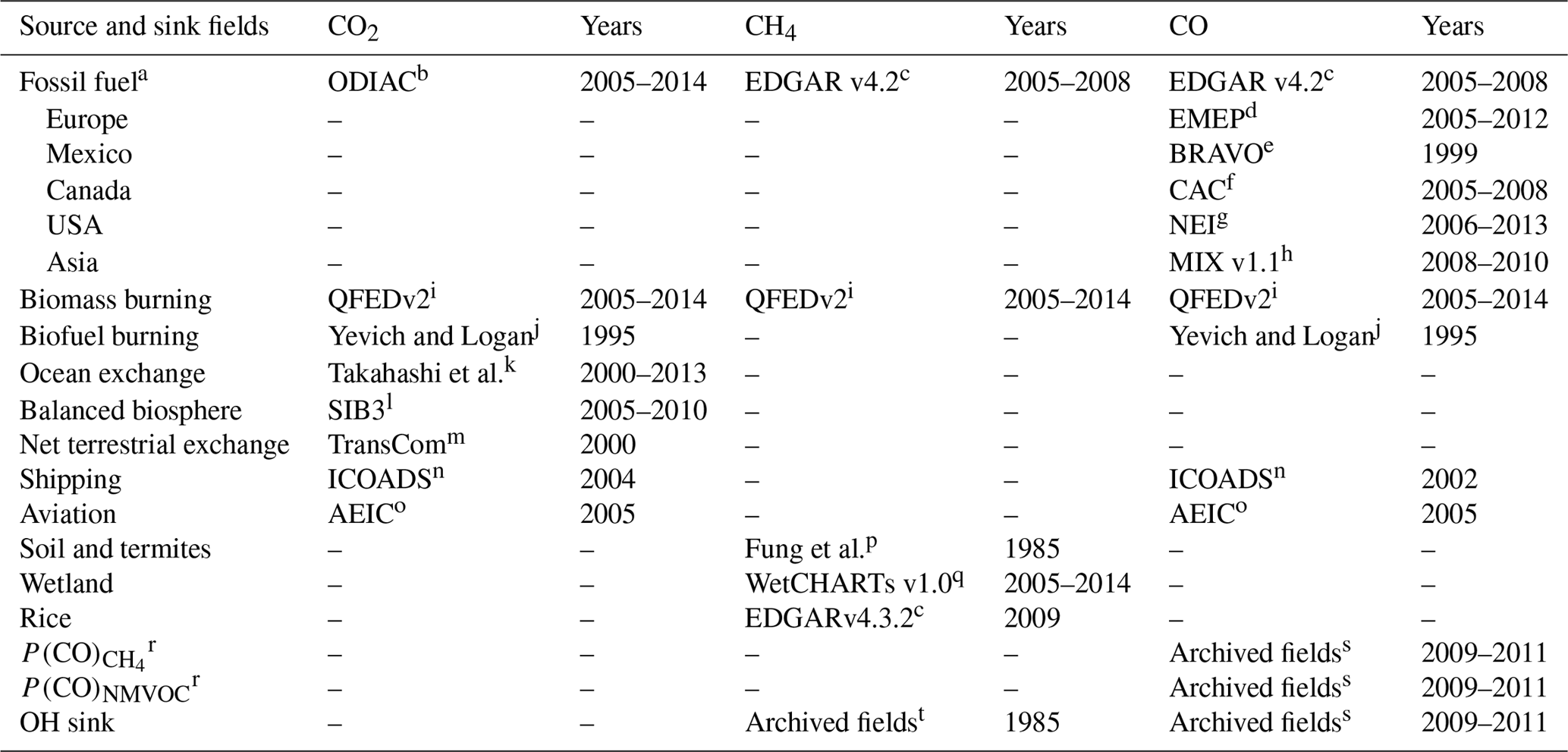
^a The anthropogenic emissions in the CO simulation had regional overwriting for the countries specified in the table. ^b Open-source Data Inventory of Anthropogenic CO₂ (Oda and Maksyutov, 2011). ^c European Commission, Emission Database for Global Atmospheric Research (http://edgar.jrc.ec.europa.eu/, last access: 19 May 2019). ^d European Monitoring and Evaluation Programme (Vestreng et al., 2007). ^e The Big Bend Regional Aerosol and Visibility Observational Study (Kuhns et al., 2005). ^f Criteria air contaminants Van Donkelaar et al. (2012). ^g National Emissions Inventory (https://www.epa.gov/air-emissions-inventories, last access: 19 May 2019). ^h Li et al. (2017). ⁱ The Quick Fire Emissions Dataset (Darmenov and da Silva, 2015). ^j Yevich and Logan (2003). ^k Takahashi et al. (2009). ^l The Simple Biosphere (Messerschmidt et al., 2012). ^m Baker et al. (2006). ⁿ International Comprehensive Ocean–Atmosphere Data Set (Lee et al., 2011). ^o Aviation Emissions Inventory Code (Stettler et al., 2011). ^p Fung et al. (1991). ^q Bloom et al. (2017). ^r The production of CO from NMVOCs and CH₄ is calculated with the GEOS-Chem full chemistry simulation from simulated monthly CO chemical production rates using biogenic NMVOC emissions from the Model of Emissions of Gases and Aerosols from Nature (MEGAN; Guenther et al., 2012), anthropogenic NMVOC emissions from the REanalysis of the TROpospheric chemical composition (RETRO) inventory (van het Bolscher et al., 2007), and biomass burning NMVOC emissions from GFEDv3 (Fisher et al., 2017). ^s Fisher et al. (2017). ^t Park et al. (2004).

While most prior work on greenhouse-gas source attribution in Australia has focussed on a single species, measurements of co-variation between species can provide useful constraints on controlling processes (Andreae and Merlet, 2001; Popa et al., 2014). CO₂, CH₄ and CO are chemically dependent, with several common sources and sinks, and changes in any one of these species can have a significant impact on the others. Table 1 highlights the source and sink processes that are common between the three gases. Both CO and CH₄ are removed through reaction with OH, the main tropospheric oxidant, leading to production of CO₂ (McConnell et al., 1971; Hewitt and Harrison, 1985; Enting and Mansbridge, 1991; Duncan et al., 2007). CH₄ oxidation leads to a near-unity production of CO (Duncan et al., 2007), and CO oxidation is responsible for about 90 % of the chemical production of CO₂ (Ciais et al., 2008; Folberth et al., 2005). All three gases are emitted during fossil fuel and biomass combustion. Because of these co-emissions that lead to coincident enhancements, ratios between the different gases can be used to identify the signature of sources including coal mining (Buchholz et al., 2016), household combustion (Zhang et al., 2000), traffic (Ammoura et al., 2014) and biomass burning (Nara et al., 2011; Parker et al., 2016; Lawson et al., 2015; Guérette et al., 2018). Nonetheless, few studies have exploited the benefits of multi-species analysis to explore co-variations and constrain relevant source and sink processes of CO₂, CH₄ and CO in Australia.

In this study, we use 6 months of observations from 2012 to 2013 collected onboard a ship that circumnavigated Australia (Sect. 2), combined with a chemical transport model (GEOS-Chem; Sect. 3), to quantify the distributions of CO₂, CH₄ and CO around Australia (Sect. 4). We investigate the role of different sources and sinks in driving the variability of these gases (Sect. 5) by identifying a series of events when we observed simultaneous enhancements in at least two of the three gases. Finally, we use these enhancements and their co-variations to identify the dominant processes driving carbon gas variability in Australia and to identify the sources that remain missing or underestimated in the GEOS-Chem model (Sect. 6).

2 Measurements

CO₂, CH₄ and CO were measured aboard the Australian research vessel Southern Surveyor operated by CSIRO (Commonwealth Scientific and Industrial Research Organisation) MNF (Marine National Facility) during seven linked voyages in the austral autumn, winter and spring of 2012 and 2013 (Table S1 in the Supplement). Figure 1 shows the locations of the ship measurements. In 2012 the voyage started in Hobart (April), after which the ship went northeast to Brisbane (Trip 1, May) then turned towards Fiji (Trip 2, May) and returned to Hobart (Trip 3, June). The 2013 trip also started from Hobart (June), after which the ship turned west towards Perth (Trip 4, June) and proceeded clockwise to Broome (Trip 5, July) and along northern Australia (August) then south to Brisbane (Trip 6, September) and back to Hobart (Trip 7, October). For the analysis, we separated the data into northbound (NB) and southbound (SB) sections for both years (Fig. 1).

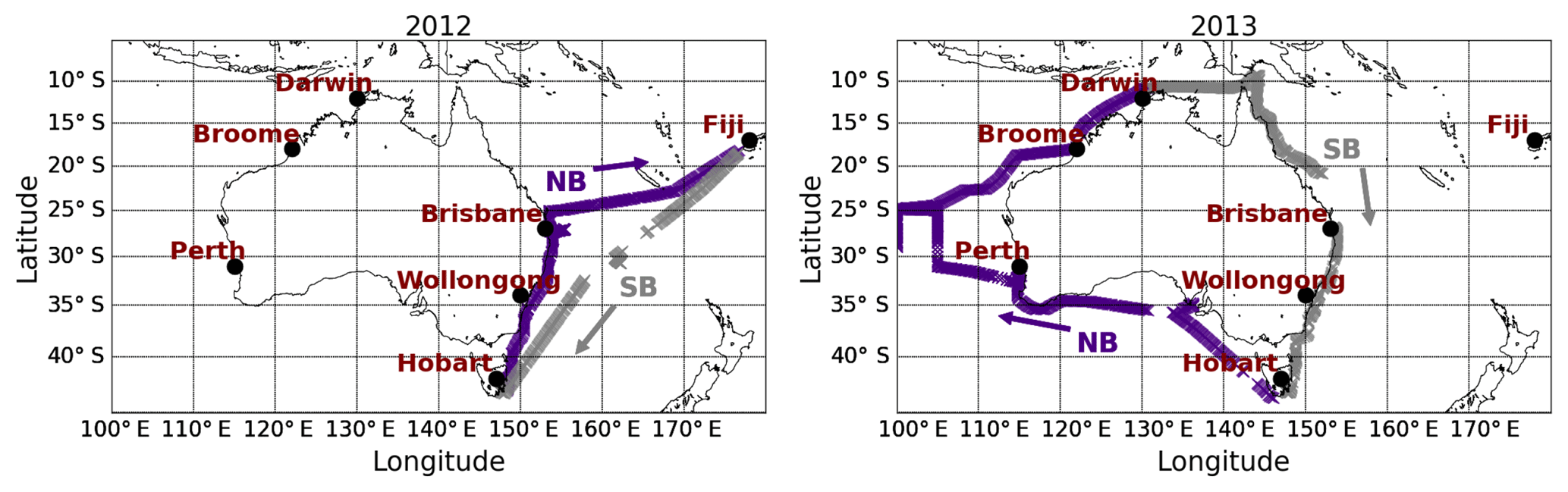
Figure 1 Locations of the shipborne measurements (purple and grey) and other sites relevant for the data interpretation (red). The ship track is separated into northbound (NB – purple; 147.5–176.6^∘ E in 2012 and 146.1–130.9^∘ E in 2013) and southbound (SB – grey; 176.6–146.1^∘ E in 2012 and 130.9–147.5^∘ E in 2013) sections to ease the interpretation of the data.

The measurements and data analysis are described in detail in a forthcoming paper in Earth System Science Data (Kubistin et al., 2019) and are briefly summarised here. The data will be available in Pangaea. All trace gas mole fractions were measured with a Fourier transform infrared (FTIR) trace gas analyser which was an early version of that described by Griffith et al. (2012) (see also Esler et al., 2000). The analyser is based around a Bruker IRcube FTIR spectrometer coupled to a 22 m multipass White cell containing the sampled air. Trace gas amounts are retrieved from the collected spectra by least-squares fitting of calculated spectra to the measured spectra in four spectral regions between 2000 and 3800 cm⁻¹ (Griffith, 1996; Griffith et al., 2012). Sampled air from the foremast of the ship flowed at 1 L min⁻¹ through the measurement cell. Single 1 s spectra were measured continuously and averaged over 5 min for the 2012 and 3 min for the 2013 voyage. The analyser was calibrated before and after the voyages against a suite of standard reference gases provided by CSIRO with assigned mole fractions on the relevant World Meteorological Organization – Global Atmosphere Watch (WMO-GAW) scales – the WMO X2007 scale for CO₂, X2004A for CH₄ and X2014 for CO. During the voyages the calibration was checked against a single calibrated working standard tank and adjusted as required.

Precision and accuracy were determined from 5 min Allan variance and 1σ reproducibility of the target tank measurements respectively. Table 2 summarises the 5 min repeatability and accuracy for each species.

Table 2 FTIR analyser 5 min repeatability and accuracy for CO₂, CH₄ and CO.

3 Model description

To investigate the sources and sinks driving the measured carbon greenhouse gases, we used the GEOS-Chem 3-D global chemical transport model (Bey et al., 2001). The meteorological inputs for GEOS-Chem come from the Modern-Era Retrospective analysis for Research and Applications, version 2 (MERRA2), reanalysis developed by the NASA Global Modeling and Assimilation Office (GMAO). We use the offline CO₂, CH₄ and CO simulations from GEOS-Chem v11-01. The CO₂ simulation is based on Nassar et al. (2010) and Nassar et al. (2013), the CH₄ simulation is based on Wecht et al. (2014), and the CO simulation is described by Fisher et al. (2017).

We ran the model at $\mathrm{2}{}^{\circ }\times \mathrm{2.5}{}^{\circ }$ horizontal resolution with 47 vertical levels from 2005 through 2016 to correct biases in the trends of the CO₂ and CH₄ simulation (Fig. S1) and from 2012 to 2013 for all results presented here. The simulations were initialised with a 10-year spin-up for CO₂ and CH₄ using 2005 as a base spin-up year and a 6-month spin-up for CO using 2005. We have found these spin-up periods to be sufficient to establish consistent spatial gradients in the atmosphere of all the tracers and total amount of each gas. The emission inventories and chemical fields used by each simulation are shown in Table 1. Where possible, we used common emission inventories for all three simulations. The three carbon gas simulations are decoupled; hence the chemical production and loss of each species (e.g. CO₂ production from the oxidation of CO, CH₄ and NMVOCs) were computed offline using archived production rates and OH concentrations. For simulations that were outside of the specified inventory time range, the model re-used the data from the closest year.

The lack of time-specific emission inventories for some emission types can introduce uncertainties in the results, but we expect these errors to be low in our simulations. CO interannual variability is mostly driven by meteorology and biomass burning, for which we used time-specific emission inventories (Fisher et al., 2017). We use time-specific emissions for CO₂ from fossil fuels, and other anthropogenic CO₂ emissions outside the time range (ships, aviation, and biofuel), have been shown to have a small contribution to both total CO₂ and CO₂ variability relative to the other sources (Nassar et al., 2010). While the terrestrial biospheric fluxes are based on climatological data, these fluxes have a larger effect in the Northern Hemisphere than the Southern Hemisphere due to the greater landmass and for periods with El Niño and La Niña events (Heimann and Reichstein, 2008). All of our measurements (April–June 2012 and June–October 2013) were collected during weak El Niño and La Niña periods. For CH₄ wetlands and biomass burning are the main drivers of interannual variability (Bousquet et al., 2006), and we used time-specific emissions for both source types.

The carbon gas simulations are all linear, and for each we included a suite of tracers tagged by source type (and, for CO, region). The tagged CO₂ simulation includes eight tracers to distinguish between source types: fossil fuel, ocean exchange, biomass burning, biofuel, balanced biosphere, net annual terrestrial exchange, shipping and aviation. The ocean exchange, balanced biosphere and net annual terrestrial exchange act both as a sink and source, while the other tracers represent only sources of CO₂.

The CH₄ tagged simulation includes 11 tracers for different source types: gas and oil, coal, livestock, waste, biofuel, rice cultivation, biomass burning, wetlands, termites, soil absorption and other combined anthropogenic emissions (e.g. energy manufacturing transformation, non-road transportation, road transportation, industrial process and product use and fossil fuel fires). The soil absorption represents a sink of CH₄, while all other tracers are sources. For CH₄, an OH sink is applied to all of the tracers; however, in contrast to the soil absorption sink there is no separate tracer for this loss.

The CO tagged simulation includes four source types: anthropogenic, biomass burning, and separate CH₄ oxidation and NMVOC oxidation. The anthropogenic tracer includes both fossil fuel and biofuel, since these sources are combined in some of the emission inventories. Stratospheric and tropospheric OH sinks are applied to all of the CO tracers. We further distinguished the anthropogenic and biomass burning tracers by region to aid in interpretation of transported influences. The transported amounts of the anthropogenic and biomass burning sources hereinafter refer to emissions from the non-Australian tagged regions as shown in Fig. 2.

For comparison to the ship measurements, model outputs were saved for grid boxes corresponding to the measured time, latitude and longitude along the ship track at the model surface level. Both the measurements and modelled output were averaged to the model temporal (20 min) and spatial ($\mathrm{2}{}^{\circ }\times \mathrm{2.5}{}^{\circ }$) resolution to calculate one average value for each unique grid-box–time-step combination. Hereinafter we will refer to this averaging method as the measurement–model averaging.

The model initial conditions and the imbalance between the modelled sources and sinks relative to the their true values created a bias in the model, which led to a difference between the modelled and measured growth rates. To compare our surface CO₂ and CH₄ measurements with the model, we corrected the modelled growth rates by first assessing offsets between the modelled and measured surface values at background stations (Barrow, Trinidad, Mauna Loa, American Samoa, Cape Grim and the South Pole; Dlugokencky et al., 2018b, a) as shown in Fig. S1. The modelled offset was then corrected with a globally averaged 13-point running mean of the difference between the modelled and measured data at the background sites. We applied this linear correction method for CO₂ and CH₄. CO was not affected by this bias due to its shorter lifetime and lack of a long-term trend.

Figure 2 GEOS-Chem tagged regions used for anthropogenic and biomass burning sources in the CO simulation. South America (56^∘ S–24^∘ N, 112–33^∘ W), Africa (48^∘ S–36^∘ N, 17^∘ W–70^∘ E), East Asia (8–45^∘ N, 70–153^∘ E), Indonesia (10^∘S–6^∘ N, 95–165^∘ E) and Australia (44–10^∘ S, 112.5–157.7^∘ E). The East Asia and Indonesia regions were used for the biomass burning source only. Regions not shown on the map are anthropogenic other and biomass burning other; these are regional tags that cover everything except the source specific tagged regions.

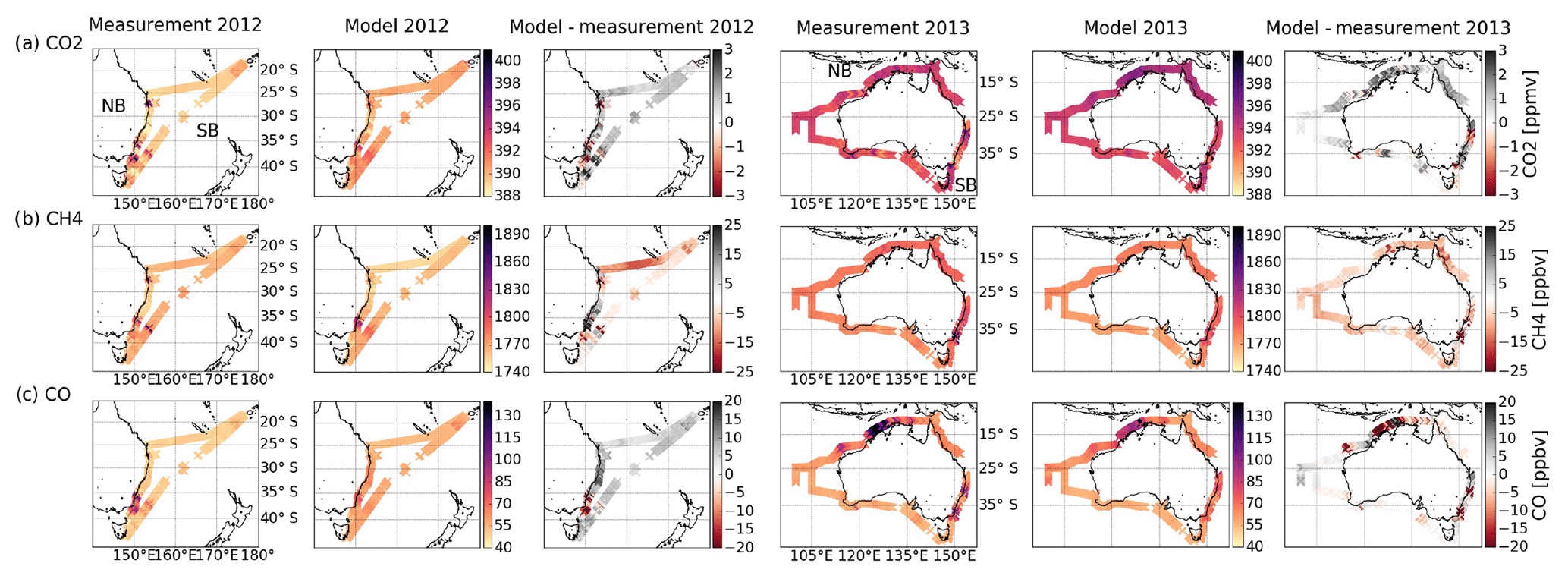
Figure 3 Measured and modelled CO₂ (a), CH₄ (b) and CO (c) concentrations from the ship cruises in 2012 (left) and 2013 (right). The measurement–model difference is also shown for each gas and ship cruise.

4 Observed and modelled CO₂, CH₄ and CO distribution around Australia

Figure 3 shows the measured and modelled CO₂, CH₄ and CO, and the difference between measurements and model, in 2012 and 2013. In both years, the three gases show similar spatial distributions, indicating their likely co-emission.

In 2012 we observed high concentrations with repeated co-enhancements of all three gases and co-enhancements of only CO₂ and CO along the eastern coast (NB part). These are all near urban and industrial areas, indicating the anthropogenic influence at these hotspots. Enhancements are also observed away from the coast on the SB part near Fiji (21^∘ S); around 38^∘ S, 153^∘ E, on the way from Fiji to Hobart; and around 41^∘ S, 150^∘ E, off the northeastern coast of Tasmania. Relative to the 2012 measurements, the 2013 enhancements were dominated by co-enhancements of only two gases, CH₄ and CO, and with more pronounced individual enhancements. No significant enhancements were observed along the southern and western coasts (2013 NB, 45–25^∘ S); however, there is a gradual increase in all three gases towards the tropics. In the northern tropical region we observe enhancements and a rise of all three gases between 12 and 20^∘ S (2013 NB). This is likely to arise from biomass burning that occurs during the late dry season (August–September), which is characterised by frequent wildfires (Edwards et al., 2006a).

The ship track was the same along the eastern coast in both years; however, most of the enhancements observed in that region differed. These results suggest that the different time period of the measurement collection (April–May 2012 compared to September 2013) and transport patterns could have affected the difference in the spatial distribution of these gases. Reanalysis data from MERRA2 meteorology show weak easterly winds along the eastern coast (30–34^∘ S) during the 2012 cruise compared to stronger westerly winds during the 2013 cruise (Fig. S2). The stronger 2013 winds may explain the more well-mixed nature of the enhancements relative to the more distinct enhancements observed in 2012.

To understand the drivers of the observed enhancements and the difference between the modelled and measured enhancements, we use modelled tracers from the GEOS-Chem model (Sect. 3). Figure 4 shows the latitudinal enhancement of the measured (black) and modelled (red) concentrations, with different modelled tracers (stacked bars) that represent sources and sinks averaged for every 2^∘ in latitude after the measurement–model averaging. The latitudinal enhancements were calculated based on the difference between the individual 2^∘ latitudinal values and the minimum value of each gas during the section in question (e.g. 2012 NB). With this calculation, the contribution of each gas and tracer is treated independently between sections, since the change of the gas is calculated relative to the section in question only. If not stated otherwise, the enhancements refer to these latitudinal enhancements that include both the broadscale change of each gas with latitude and the enhancements due to different local or regional sources.

Figure 4 Measured (black) and modelled (red) CO₂, CH₄ and CO latitudinal enhancements (lines) and modelled source contributions (stacked bars) in 2012 (left) and 2013 (right) for the northbound (NB) and southbound (SB) sections of the ship cruises. All the data were averaged in 2^∘ latitude bands after the measurement–model averaging. The enhancements were calculated based on the difference between the individual 2^∘ latitudinal values and the minimum value during each section.

4.1 Anthropogenic sources

The model reproduced the observed eastern coast enhancements in 2012 (Fig. 3) and primarily attributes them to anthropogenic sources, including fossil fuel for CO₂, coal, livestock, oil, gas and waste for CH₄, and fossil and biofuel for CO (25–44^∘ S; Fig. 4). A previous study by Buchholz et al. (2016) also showed that anthropogenic sources have a strong impact on measurements collected on the eastern coast. The wind patterns and the modelled sources show that the high concentrations observed at 38^∘ S, 153^∘ E, downwind from the southeastern Australian coast, are transported anthropogenic sources for all three gases. The model tracers show the same source influences in this downwind region as those observed nearer to the eastern coast; however, the model underestimates the strength of the transported enhancements due to either underestimated emissions or the influence of numerical diffusion on transport. The SB voyage occurred several weeks after the NB voyage up the eastern coast, so enhancements with similar source profiles do not necessarily indicate the same enhancement events. For CH₄, the transported amounts observed in the downwind region were higher than those observed along the coast during the NB leg (Fig. 3), indicating that even if these enhancements derive from the same urban source, the source was stronger during the later (SB) trip than during the earlier (NB) trip. The high measured concentrations near Fiji arise from a combination of transported biomass burning and anthropogenic sources, while the enhancements at 41^∘ S, 150^∘ E, are due to transport from the northeastern coast of Tasmania. The main source driving the observed CH₄ enhancement along the Tasmanian coast is emission from livestock, in contrast to the strong coal burning emissions observed along the southeastern mainland coast.

The measurements along the northwestern and northern coasts were taken in July–August (NB 2013), when the ITCZ is situated to the north of Australia (Fig. S3) and Australia is chemically isolated from the Northern Hemisphere; however, for long-lived gases like CO₂ and CH₄, we expect interhemispheric transport to induce a latitudinal gradient throughout the year. We attribute a significant part of the CO₂ fossil fuel and anthropogenic CH₄ sources in the northern parts of Australia to transport from the Northern Hemisphere due to their gradual increase and diffuse enhancements. Based on the regionally tagged CO tracers, the largest contribution to the anthropogenic sources in the northern parts is attributed to transport from Asia, Indonesia and elsewhere in the Northern Hemisphere (Fig. 4; NB section, 2013).

4.2 Natural sources

Southern Hemisphere biomass burning is more pronounced in September (2013 SB) than in April–May (2012 NB), and the model shows a larger influence from both local and transported biomass burning for all three gases along the eastern coast in 2013 than in 2012.

The model captured the rise of all three gases in the tropical regions but did not fully reproduce the strength of the enhancements. For all three gases, it underestimated the source from biomass burning, except for an overestimated CO enhancement around 12^∘ S. These biases suggest that, despite using the year-specific biomass burning emissions from the Quick Fire Emissions Dataset (QFED) inventory, there are still uncertainties in biomass burning emissions that affect simulation of carbon gases. Based on the modelled CO tracers (Fig. 4), the biomass burning enhancements along the northern coast (NB, SB 2013; 10–25^∘ S) mainly originated from Australia. Transported biomass burning from Africa was present along the western coast (NB 2013; 25–35^∘ S), while the eastern coast (SB 2013; 25–45^∘ S) was affected by biomass burning from both Africa and South America.

To further examine the transport from fires, we used data from the MODIS (Moderate Resolution Imaging Spectroradiometer) instrument and global winds from the MERRA2 reanalysis. Figure S4 shows the total fire pixels from MODIS detected between 3 weeks and 1 week prior to each of the seven ship cruises segments in 2012 and 2013 along with monthly mean wind fields. Figure S4 suggests that South American fires prior to the 2013 SB transit along the eastern coast (September 2013) were stronger than before the 2013 NB transit along the western coast (July 2013). This explains the greater South American biomass burning influence along the eastern coast relative to the western coast, observed by the model using QFED biomass burning emissions, that are based on products from MODIS. Strong fires were also observed in Africa prior to both the NB and SB transits in 2013. However, the fires before the SB transit were more spread out along the eastern and southern areas of Africa, and more coincident with the westerly winds, relative to the fires observed during the NB transit. This resulted in more biomass burning emission transport to the Australian eastern coast during September and less to the western coast in July.

4.3 Latitudinal gradients and background regions

The model indicates that for CO₂, the increase along the southern and western coasts is driven by fossil fuel emissions, biomass burning, changes in the biosphere and also a decrease in the ocean sink, which together result in higher CO₂ in the northern parts of Australia. For CO, the latitudinal increase is mainly due to increased biomass burning and NMVOC oxidation, while for CH₄, both anthropogenic and natural sources showed a gradual increase with latitude.

Based on the measurements along the southwestern, western and northwestern coasts (where few enhancements were observed), we observe a background latitudinal gradient with a standard error of 0.019 ± 0.003 ppm per degree for CO₂, 0.34 ± 0.02 ppb per degree for CH₄ and 0.82 ± 0.05 ppb per degree for CO. The model showed a stronger latitudinal gradient of 0.098 ± 0.005 ppm per degree for CO₂, 0.61 ± 0.02 ppb per degree for CH₄ and 1.09 ± 0.07 ppb per degree for CO. The difference between the measured and modelled latitudinal gradients was due to either the imbalance of the different sources and sinks used in the model (e.g. weaker Southern Hemisphere sources in the model) or inaccurate transport (e.g. weaker latitudinal transport).

For both years, we identified sections where no enhancements were observed and used these to quantify background amounts for the gases. During 2012, all three gases were the least variable in the NB section from Brisbane to Fiji in the Coral Sea and in the SB section between 155 and 173^∘ E in the Tasman Sea. During 2013 no enhancements were observed sailing west in the NB section over the Indian Ocean. The locations of these regions are shown in Fig. 5a and b. The background section mean mole fractions of the gases, both measured and modelled, are shown in Fig. 5 and in Table S2. The measurements in the three regions are consistent with the expected temporal and latitudinal variations in these gases. The amounts of all three gases were higher in the Indian Ocean than in the two other regions, due to the interannual and seasonal variability between the periods when the measurements were collected (July 2013 compared to May–June 2012). CH₄ and CO were higher in the Tasman Sea (June 2012) relative to the Coral Sea (May 2012), presumably due to the 1-month difference in the measurement timing. CO₂ showed minimal difference between the Tasman Sea and Coral Sea background regions, but with lower values in the Tasman Sea, presumably due to the weaker oceanic sink closer to the tropics (Takahashi et al., 2009). The model overestimated the background values for CO₂ and CO and underestimated the background CH₄ in all three regions. The measurement–model residuals were consistent for each in all three background regions, showing that the sources or sinks acting on a broader scale need further constraints.

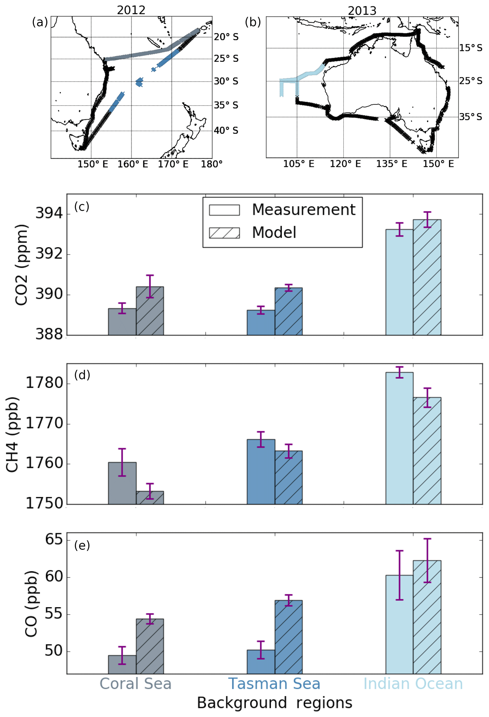
Figure 5 Measured and modelled CO₂, CH₄ and CO concentrations from the ship cruises in different background regions with 1 standard deviation. The location of the sections where background values were observed are shown on the map. The measurements in the Coral Sea (grey) were collected during May 2012, in the Tasman Sea (dark blue) during June 2012 and in the Indian Ocean (light blue) during July 2013.

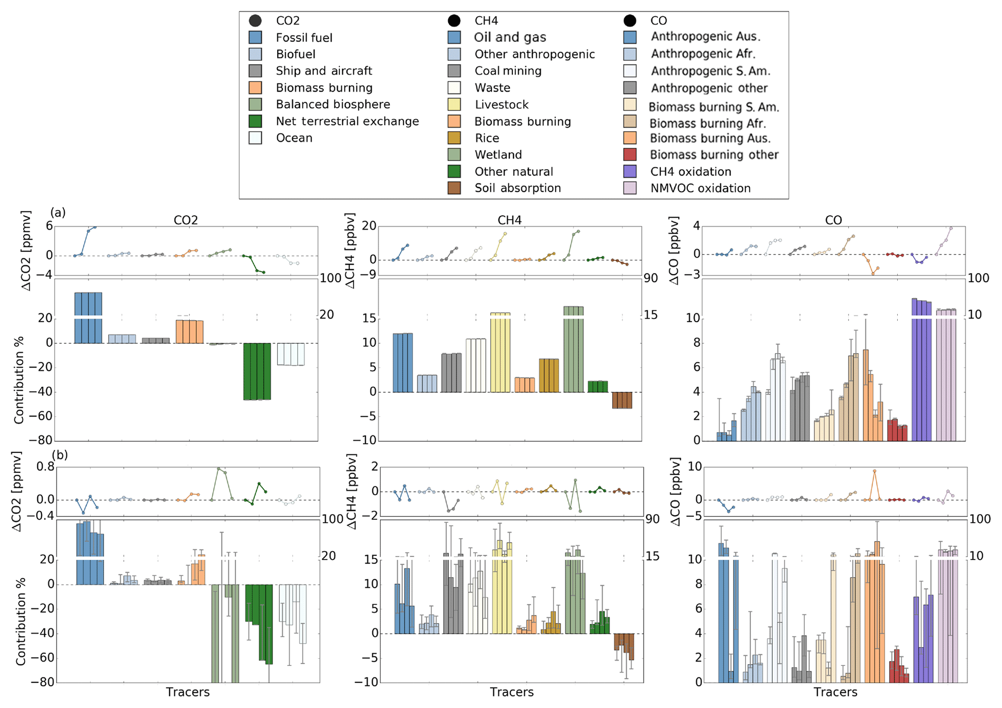
Figure 6 CO₂, CH₄ and CO tracer contribution across the four measurement section in 2012 and 2013 (2012 NB, 2012 2B, 2013 NB and 2013 SB; from left to right) for the background (a) and enhancements (b). We separated out the total amount of each gas into background values and enhancements to examine the impact of different temporal and spatial scales on the change of the sources. The bottom plots show the contribution of each tracer during a specific trip, while top plots show the change of each tracer across the four sections relative to the first section (2012 NB). The contributions are calculated based on the median for each section, and the uncertainties represent the 25th (lower error bar) and 75th (upper error bar) percentile.

5 Source variability with respect to scale

To assess how much each source and sink contribution varied at short (local) versus long (regional) scales along the four measurement sections (NB and SB, 2012 and 2013), we separated the total amount of each gas into background values (Fig. 6a) and enhancements (Fig. 6b). The bottom plots in Fig. 6a and b represent the percentage change of each model tracer relative to the tracers during a given measurement section, while the top plots represent the absolute change in a given tracer relative to the first measurement section (2012 NB). All the contributions are calculated along the ship track; hence results discussed here refer to CO₂, CH₄ and CO in the Australian region only.

Figure S5 illustrates the process of separating the measured and modelled data into background values and enhancements. We first averaged the data into 0.1^∘ latitudinal values (after the measurement–model averaging described in Sect. 3), and for each section, we calculated the change of all three gases from one latitude bin to another. Based on these changes (e.g. δCO; Fig. S5) we examined different values to choose a threshold value that most clearly separates the background regions from the enhancements for each section separately. For changes below the threshold value, the measured and modelled points were classified as background regions and enhancements if the change between the points was above the threshold value. The threshold values for each section can be found in Table S3. The background values were additionally filtered to only include data within 1 standard deviation of the mean. Due to the influence of the latitudinal gradient on the background values, we used a moving mean and standard deviation. Finally, we calculated the relative values of the enhancements based on the difference between the amount of gas at each individual 0.1^∘ latitudinal value and the minimum value during the specified sections, as in Sect. 4. Table S4 provides a statistical comparison of the measured and modelled total, background-only, and enhancement-only values.

The source and sink contributions to the background (Fig. 6a) values showed the same behaviour as the source and sink contributions to the total amounts (Fig. S6 and Table S5), but with less variability. Only the CO local sources (Australian anthropogenic and biomass burning emissions) and African biomass burning showed any difference between background and total amounts. As a result, only the background values are discussed here, but the background analysis also applies to the total amount of each gas.

Our model results suggest that fossil fuels followed by biomass burning contribute the most to background and total CO₂ (Fig. 6a). Both the biosphere and the ocean were net sinks during all four measurement sections, with a net contribution ($-\mathrm{64}\pm \mathrm{0.1}$ %, averaged along the four sections with 1 standard deviation) that was about 6 % less than the amount of CO₂ emitted from fossil fuels alone (69.9±0.2 %).

For CH₄, wetlands were identified as the biggest background source followed by emissions from livestock, oil, gas and waste. Emissions from coal mining and rice were smaller but still important. The remaining sources contributed less than 3 % each. The CH₄ soil absorption tracer represents a sink that is similar in magnitude to the CH₄ source from biomass burning, as seen previously by Dalal et al. (2008) for Australia, and their quantification of the contribution of different anthropogenic sources is consistent with our findings here.

For CO, chemical production from CH₄ and NMVOCs was the biggest contributor to the background and total amounts (70 ± 2 %). This shows that the CO burden in Australia and the Southern Hemisphere is largely controlled by secondary CO production, consistent with findings from Zeng et al. (2015) that biogenic emissions provide the largest CO background contribution. Biomass burning, both transported to and from Australia, is responsible for 14 ± 1 % of the total simulated CO, from which 68 ± 12 % is attributed to transported biomass burning, with the highest amounts originating from Africa, followed by South America, as seen previously by Gloudemans et al. (2006) and Ridder et al. (2012). Anthropogenic processes contribute 16 ± 2 % to the total CO, 90 ± 6 % of which is transported (mainly from South America).

In the model, the CO₂ and CH₄ enhancements (Fig. 6b) were generally driven by similar sources to the background amounts (Fig. 6a). For CO₂, the biospheric influence is more pronounced in the enhancements than in the background. For CH₄, anthropogenic sources (especially coal mining) contribute more to the enhancements than to the background, while wetlands (the biggest contribution to the CH₄ background) contribute considerably less to the enhancements. Fraser et al. (2011) showed that for years prior to 2012 at a single site on the eastern coast (Wollongong), coal mining was the largest source of CH₄ enhancements above the background (60 %). Our results suggest that coal mining (21 %) and emissions from livestock (28 %) are the largest contributors to the enhancements along the eastern coast in 2012 (leftmost grey bar in Fig. 6b). Although the different analysis time periods might have influenced these differences, the main reason for the lower coal mining contribution in our results is due to the wider measurement region along the eastern coast used to quantify these contributions.

The CO enhancements were less affected by the tracers that contributed the most to the background, since these tend to be spatially uniform sources. While total and background CO amounts were dominated by secondary sources (CH₄ and NMVOC oxidation), the enhancements were largely driven by primary CO emissions from biomass burning and anthropogenic sources, with stronger influence from Australian sources than from long-range transport. The CO enhancements also showed significant regional variability.

For all three gases, the enhancements above the background were dominated by temporally and spatially variable sources and sinks, displaying significant variability both within each section and between the four sections. In contrast, the CO₂ and CH₄ sources and sinks contributing to the background showed minimal variability between the four measurement sections. The CO background sources varied somewhat between the four sections (Fig. 6a), due to the shorter CO lifetime, but this background variability was still less than the variability seen in the CO enhancements (Fig. 6b).

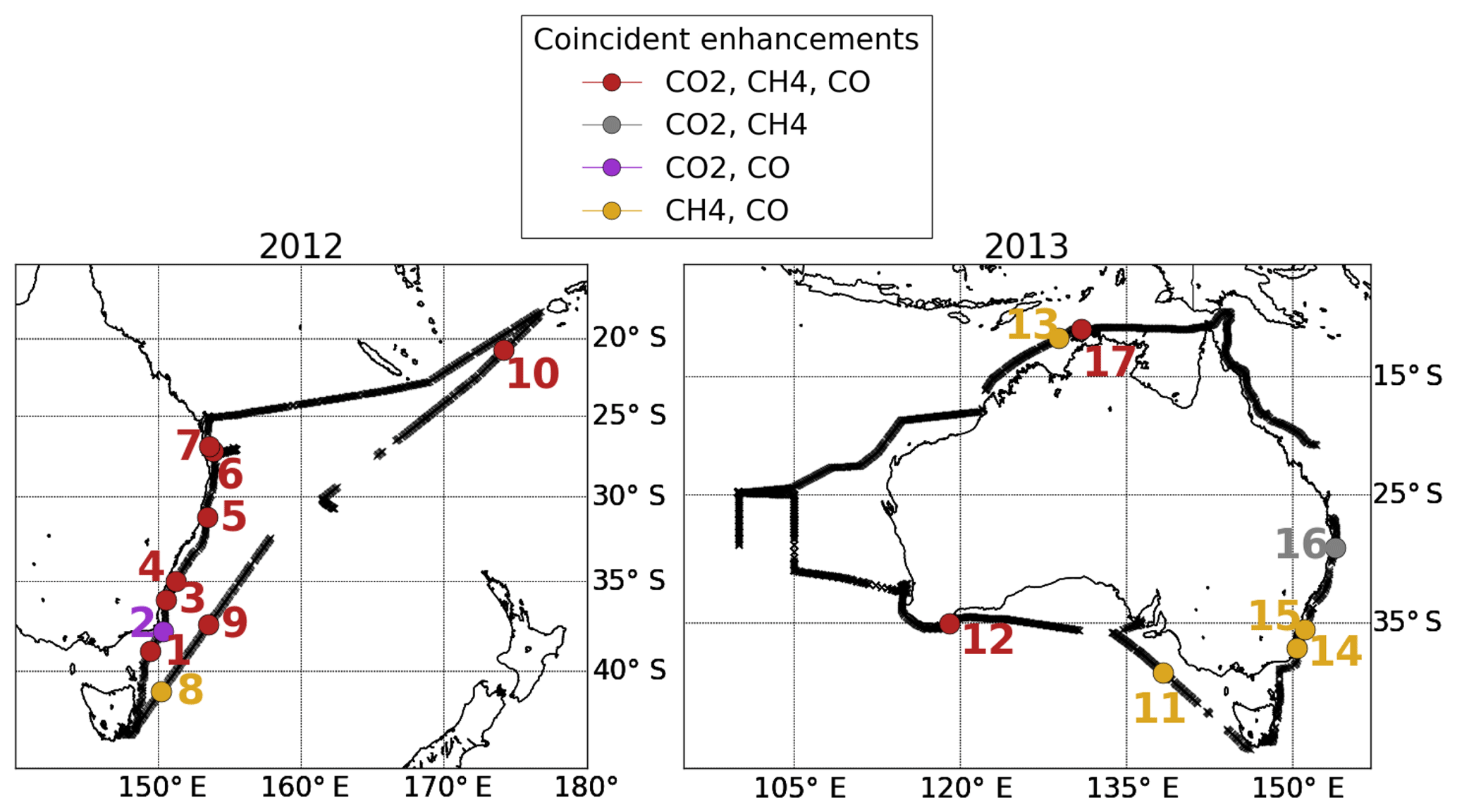
Figure 7 Location of the 17 events during which we observed co-enhancements of CO₂, CH₄ and CO. The red numbers represent events with coincident enhancements in all three species, grey numbers represent co-enhancements in CO₂ and CH₄ only, purple numbers represent coincident enhancements in CO₂ and CO only, and yellow numbers represent coincident enhancements from CH₄ and CO only. The black line represents the measurement track during 2012 and 2013.

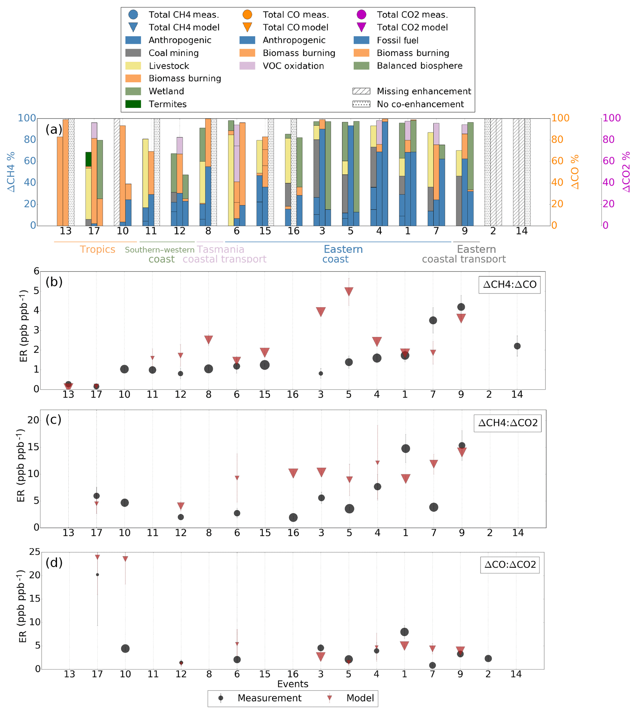
Figure 8 (a) shows the contribution of different tracers (stacked bars) to the modelled enhancements of CH₄ (first bar), CO (second bar) and CO₂ (third bar) for the 17 events when we observed co-enhancements of the measured gases. (b–d) show the measured (circle) and modelled (triangle) enhancement ratios for ΔCH₄:ΔCO, ΔCH₄:ΔCO₂ and ΔCO:ΔCO₂; the error bars represent the standard error. The size of the markers represents the correlation coefficient between the species during the coincident enhancements. Enhancement ratios and tracer contributions from the model are only shown for events when the model also saw evidence of co-enhancement. The events are ordered based on both the source type and region where it occurred.

6 CO₂, CH₄ and CO correlations and co-enhancements

The spatial distributions of the three carbon gases (Fig. 3) showed similar enhancement patterns, suggesting that the gases were co-emitted. From these coincident and co-located enhancements, we estimated enhancement ratios (ERs) from both the measured and modelled values, averaged into 0.1^∘ latitudinal bands, across the four different sections after the measurement–model averaging. We defined the ER between two species as the slope between the enhancements of the two species calculated using linear regression (Turnbull et al., 2011). For the purpose of calculating the ER, the enhancement was defined as the difference between the maximum and minimum value of each gas during the specific co-enhancement event. This definition removes the potential impact introduced by the changing background concentrations between the three gases. Unlike the enhancements discussed earlier, the enhancements used to define the ERs are not affected by latitudinal gradients, and they are not influenced by the changes due to latitudinal or other broadscale changes.

We use this information to evaluate mismatches between the model and the observations and specifically to determine whether (1) the modelled source profile is correct (i.e. same ERs as in the observations) but with the wrong magnitude for the source or (2) the model has a missing or incorrect source (different ERs). Figures S7 and S8 show species–species linear regressions for events when we observe coincident enhancements in at least two gases.

From the measurements, we found evidence of co-enhancements during 17 events. The locations of these events are shown in Fig. 7. The ERs and correlation coefficients are also summarised in Table S6. All events except event 3, 4, 12 and 17 showed correlations of r>0.80 between the species during the coincident enhancements. The 2012 measurements generally showed co-enhancements of all three gases, while the 2013 data generally showed individual enhancement or enhancements of only two species. Of the 17 events identified in the measurements, the model reproduced co-enhancements for 14 (all except 2, 14 and the CH₄ enhancement in 10) but underestimated the magnitude of most enhancements.

6.1 Enhancement ratios and source signatures

Figure 8a shows the modelled sources that contributed to co-enhancement events from which we derived enhancement ratios. The measured ERs (Figure 8b–d) are shown as circles, with triangles for the corresponding modelled ERs (only for events when the model simulated similar co-enhancements). The difference between the measured and modelled CO₂, CH₄ and CO enhancements and ERs during each event is shown in Fig. S9.

The modelled tracers suggest that there is a relationship between the ΔCH₄:ΔCO ERs and the sources driving the enhancements. Both the measurements and model showed low ERs for events caused by natural processes (mostly biomass burning; orange), higher ERs for events with mixed natural and anthropogenic signatures, and the highest ERs for events dominated by anthropogenic sources (blue and grey). The balance of sources varies regionally, so the lowest ERs were observed in the tropics due to the impact of stronger natural emissions. Higher ERs were seen along the southern and western coasts due to the influence of both natural and anthropogenic sources. We found the highest ERs along the eastern coast due to the impact of different industrial areas.

The patterns are similar for ΔCH₄:ΔCO₂ ERs, with higher ERs from anthropogenic processes. For ΔCO:ΔCO₂, we found the highest ER for event 17, which is driven by biomass burning, suggesting that biomass burning is the process that produces the most CO relative to CO₂ and CH₄. The lowest measured ΔCO:ΔCO₂ ERs were identified for events 12 and 7, which derived from anthropogenic sources for both gases combined with additional biomass burning and volatile organic compound (VOC) oxidation for CO and biosphere influence for CO₂.

The co-enhancements and events detected along the eastern coast highlight the anthropogenic influence in this part of Australia. Ten events (events 1, 2, 3, 4, 5, 6, 7, 14, 15 and 16) were identified along the eastern coast, all with dominant anthropogenic signature, and one event (event 9) was detected 400 km off the eastern coast. The measured and modelled ERs seen during event 9 showed similar values, with the modelled tracers suggesting that this enhancement has an anthropogenic origin and originates from the eastern coast due to the similar source composition. The ERs along the eastern coast were mainly overestimated by the model.

One event (event 8) was observed off the northeastern coast of Tasmania. Despite being located in the vicinity of the events observed along the eastern coast, the ΔCH₄:ΔCO ER for event 8 is lower than most of the enhancements observed along the eastern coast. In contrast to the CH₄ source contribution along the eastern coast, the main CH₄ sources for event 8 are wetlands and livestock, while most of the events along the eastern coast had coal mining as a dominant source, pointing to a weaker anthropogenic influence from the northeastern coast of Tasmania relative to the Australian eastern coast.

The biggest difference between the measured and modelled ERs when CH₄ was co-emitted was during events 3, 4, 5, 7 and 16 (all located along the eastern coast). The model overestimated the ERs for events 3, 4, 5 and 16 for both ΔCH₄:ΔCO and ΔCH₄:ΔCO₂, while for event 7, it overestimated the ΔCH₄:ΔCO₂ and underestimated the ΔCH₄:ΔCO ER. All the events with the highest modelled ERs (when CH₄ is emitted) have coal mining as the dominant source, which suggests that this source was overestimated in the model for events 3, 4, 5, 7 and 16. The fact that the ΔCH₄:ΔCO ER during event 7 was underestimated shows that the biomass burning source of CO was too high relative to CH₄ and CO₂, since the ΔCO:ΔCO₂ ER was also overestimated by the model.

Prior work on CH₄ showed that globally in EDGAR v4.2 anthropogenic emissions from livestock, landfills and other minor sources are underestimated, while oil, gas and coal emissions are overestimated, but with underestimates in North America (Wecht et al., 2014; Turner et al., 2015) and overestimates in China (Bergamaschi et al., 2013). However, no similar analysis has been done for Australia; hence the sign and the magnitude of this bias in the Australian region are unknown. Based on co-variations between CO₂, CH₄ and CO along the eastern coast, we show that the source from coal mining is also overestimated in Australia. The only event when coal mining was a dominant source and the model showed a similar ER to the measurements was during event 9.

Along the southern and western coasts, the sources reflect a mixture of anthropogenic and natural emissions. Relative to the eastern coast, the ERs were lower for these events (events 11 and 12). The source signatures were similar to some events observed along the eastern coast with mixed biomass burning and anthropogenic sources, like events 6 and 15. During event 12 the model showed a similar ER to the measurements for ΔCO:ΔCO₂ and overestimated the ΔCH₄:ΔCO₂ ER. The ΔCH₄:ΔCO ERs were overestimated for both events 11 and 12. This overestimation and the greater difference between the measured and modelled CO enhancements relative to the CO₂ and CH₄ enhancements (Figure S9, Supplement) suggest that the source from biomass burning was underestimated in the model for both events, since biomass burning was the dominant CO source.

The northern coast and tropics were mostly influenced by biomass burning (events 10, 13 and 17). The model reproduced the ΔCH₄:ΔCO ER during event 13 (when no CO₂ enhancement was observed), while for event 17 it reproduced the ΔCH₄:ΔCO ER, slightly underestimated the ΔCH₄:ΔCO₂ ER and overestimated the ΔCO:ΔCO₂ ER. These differences were potentially caused by the coarse 2^∘ × 2.5^∘ resolution of the GEOS-Chem model. With such coarse resolution, the strength of local sources is diffused. The resolution likely affected event 17, when the observed enhancements were weaker and less distinct than those observed during other events. The model overestimated the ΔCO:ΔCO₂ ER during event 10. Based on the measured–modelled enhancement difference (Fig. S9), the CO enhancement was overestimated by the model and the CO₂ enhancement underestimated. The difference in the modelled ER is hence likely due to the overestimated strength of the biomass burning source in CO and its underestimation in CO₂, since it was shown as a dominant source. The model did not reproduce the CH₄ enhancement at all for event 10, pointing to a missing source in the model.

6.2 Summary of co-enhancements and implications for missing sources

Using the derived ERs more broadly and linking them to a specific source signature is challenging due to the mixture of sources during the co-enhancement events. From the 17 events, only one (event 13) showed contribution from only one source (biomass burning), while all the other co-enhancements were due to a mixture of sources. However, we found these ERs to be representative in identifying the prevailing processes driving the sources (natural, anthropogenic or mixed), in determining sources that are underestimated or overestimated in the model, and in identifying the source signatures not captured by the model.

Our biomass burning ER agrees well with known enhancement ratios. The event 13 ER showed a value of 0.27 ppb ppb⁻¹ for ΔCH₄:ΔCO, similar to the 0.15–0.44 ppb ppb⁻¹ range of enhancement ratios from previous studies (Mühle et al., 2002; Mauzerall et al., 1998) but higher than previously measured emission ratios (0.04–0.06 ppb ppb⁻¹, Lawson et al., 2015; Guérette et al., 2018; Paton-Walsh et al., 2014; Smith et al., 2014). This is due to the faster photochemical destruction of CO by OH relative to CH₄. The influence of chemical loss leads to lower CO values in the tropics, which result in higher ΔCH₄:ΔCO enhancement ratios in comparison to emission ratios.

Events when the model showed similar ERs to the measured ones (events 1, 4 and 9) with a strong anthropogenic signature showed a range of ratios of 1.6–4.2 ppb ppb⁻¹ for ΔCH₄:ΔCO, 8–15 ppb ppm⁻¹ for ΔCH₄:ΔCO₂ and 3.3–8 ppb ppm⁻¹ for ΔCO:ΔCO₂. These values agree with the range of previously measured ERs from urban and industrial emissions (0.3–13 ppb ppb⁻¹ for ΔCH₄:ΔCO, 9.8–61 ppb ppm⁻¹ for ΔCH₄:ΔCO₂ and 1.3–37.4 ppb ppm⁻¹ for ΔCO:ΔCO₂; Buchholz et al., 2016; Niwa et al., 2014; Harris et al., 2000; Chi et al., 2013; Xiao et al., 2004; Bakwin et al., 1995; Takegawa et al., 2004; Sawa et al., 2004; Wada et al., 2011; Lai et al., 2010; Ammoura et al., 2014; Lin et al., 2015).

The highest measured anthropogenic ER, when CH₄ was co-emitted, was during event 9, with significant contribution from coal burning (4 ppb ppb⁻¹ for ΔCH₄:ΔCO and 15 ppb ppm⁻¹ for ΔCH₄:ΔCO₂). Our values are lower than the ERs reported by Buchholz et al. (2016) (13 ppb ppb⁻¹, 61 ppb ppm⁻¹) at a single measurement site (Wollongong); however, they noted that their values were higher than known ERs due to the close proximity of the measurement site to coal seams and related mining. Additionally, for our event 9, we also observe other sources types (e.g. livestock for CH₄) that would impact the overall ERs.

Events with a mixture of natural and anthropogenic sources (events 11, 12 and 17), with values close to the modelled ERs, showed a range of ratios of 0.2–1 ppb ppb⁻¹ for ΔCH₄:ΔCO, 2–6 ppb ppm⁻¹ for ΔCH₄:ΔCO₂ and 1.4–20 ppb ppm⁻¹ for ΔCO:ΔCO₂, similar to the reported values of 0.3–2.2 ppb ppb⁻¹ for ΔCH₄:ΔCO, 19 ppb ppm⁻¹ for ΔCH₄:ΔCO₂ and 0.01–29.30 ppb ppm⁻¹ for ΔCO:ΔCO₂ (Buchholz et al., 2016; Lin et al., 2015; Lai et al., 2010; Russo et al., 2003).

Based on our derived ERs, we identified missing sources in the model during events 2, 14 and 10. Events 2 and 14 correspond to a similar region along the eastern coast, but with 1-year difference. Both events were observed along the eastern coast, where we found the most anthropogenic co-enhancement events. Event 2 was observed in 2012, and its measured ER was similar to the ER corresponding to event 5. This suggests that this missing source is a combination of anthropogenic (fossil and biofuel) emissions, with an additional natural biosphere source for CO₂. The ER for event 14 in 2013 shows a value closest to the modelled ER during event 4, which was observed in the same region in 2012. The modelled sources point mainly to an anthropogenic signature of the missing source for both CH₄ (oil, gas, coal mining and livestock) and CO (fossil and biofuel) during this event. The measurements showed enhancements for all three gases during event 10, but the model failed to capture the CH₄ enhancement. The sources of CO₂ and CO suggest that the missing CH₄ source is a combination of biomass burning and anthropogenic sources, with biomass burning being the dominant source, while the similarity between the measured ERs during events 10, 6 and 11 suggest that there is also a significant livestock contribution.

7 Conclusions

We have used in situ FTIR measurements collected in 2 consecutive years from a ship that circumnavigated Australia to construct near-surface atmospheric CO₂, CH₄ and CO distributions around Australia. Using tagged simulations from the GEOS-Chem model, we estimated the contribution of different sources to the total and background amounts of each gas and identified the drivers of their short-term enhancements. Co-variations between the different measured and modelled gases were used to identify common sources of all three carbon greenhouse gases and to understand the origin of the differences between measured and modelled quantities. Based on the co-variations, we constrained relevant processes for all three gases.

We found significant regional variability in the dominant source contributions along the Australian coast. The Australian eastern coast was dominated by anthropogenic sources, the southern and western coasts showed a mixture of anthropogenic sources and biomass burning, and the northern coast was influenced primarily by natural sources (biomass burning) for CO, anthropogenic sources (fossil fuel) for CO₂, and a mixture of anthropogenic and natural sources for CH₄. The clean air characteristic of the tropospheric background was observed away from the coast in the Indian Ocean, Coral Sea and Tasman Sea. From the measurements in the Indian Ocean, we found that the background values of all three gases increase towards the tropics with latitudinal gradients of 0.019 ± 0.003 ppm per degree for CO₂, 0.34 ± 0.02 ppb per degree for CH₄ and 0.82 ± 0.05 ppb per degree for CO.

Our model results suggest that fossil fuels (69.9 ± 0.2 %) followed by biomass burning (18.7 ± 0.1 %) contributed the most to total CO₂ and its background values. For CH₄, wetlands (33.1 ± 0.1 %) were identified as the largest background source, followed by emissions from livestock (20.59 ± 0.05 %), oil and gas (12.01 ± 0.03 %), and waste (10.90 ± 0.01 %). For CO, secondary chemical production from CH₄ and NMVOCs was the biggest contributor to the background (70 ± 2 %). Episodic enhancements in CO₂ and CH₄ were largely driven by similar sources to the background amounts, although for CH₄, the anthropogenic sources influenced the enhancements more strongly than the background. The CO enhancements were driven by primary CO emissions from biomass burning and anthropogenic sources, with stronger influence from Australian sources than from transported sources. While the short-term enhancements were driven by local sources, overall we found that sources transported from other regions greatly affect the total amounts of these gases in Australia. For CO, 68 ± 12 % of the total biomass burning contribution is attributed to transported amounts, mainly from Africa and South America, and 90 ± 6 % of the total anthropogenic contribution is from transported amounts, with the greatest contribution from South America. Transport from the Northern Hemisphere was observed closer to the tropics from regions including Asia, Indonesia and elsewhere in the Northern Hemisphere.

We observed similar enhancement patterns for CO₂, CH₄ and CO along the measurement path, pointing to coincident enhancements of these gases. Based on these coincident enhancements, we derived measured and modelled enhancement ratios (ERs) for 17 events, and we used the model to identify the source contributions for each event. We found the most events along the eastern coast, followed by the tropical northern coast. The ΔCH₄:ΔCO₂ ERs showed dependence on both source type and region. We found low ERs for events caused by natural processes, such as biomass burning (tropics and northern Australia), higher ERs for events with mixed natural and anthropogenic sources (southern and western coasts) and the highest ERs for events dominated by anthropogenic sources (eastern coast). The ΔCH₄:ΔCO ERs also showed higher values for the enhancements that mainly originated from anthropogenic processes. For ΔCO:ΔCO₂ we found the highest ERs for events driven by biomass burning and the lowest ERs for events that derived from a combination of anthropogenic sources for both gases along with biomass burning and VOC oxidation for CO and biosphere influence for CO₂. For events when the model showed similar ERs to the measurements, our ratios agreed well with known ERs.

Assumptions in the simulations, a lack of time-specific emissions and the influence of numerical diffusion on the transport can all introduce uncertainties in the modelled results. Our model results captured the distribution of the measured amounts and the main sources driving the changes of all three gases, but some discrepancies remain. Based on the measured and modelled ERs, we identified the source signature of the events that were not reproduced by the model. We found coal burning to be overestimated for CH₄ and biomass burning to be generally underestimated for all three gases, although with CO overestimates during some events. We attributed the missing sources during events that were not reproduced by the model to mainly anthropogenic sources for CO and CO₂ and oil, gas, coal and livestock for CH₄. The exception is along the tropical northern coast, where biomass burning is the main underestimated source for all three gases.

Processes driving carbon greenhouse-gas changes in Australia have a large impact on the global carbon cycle and our climate (Poulter et al., 2014; Ma et al., 2016; Haverd et al., 2017); hence, constraints on these processes are essential for predicting future climate change scenarios. Our results show that focussing on simultaneous measurements rather than individual species provides useful additional information in estimating source profiles and contributions. We have shown that the co-variation in CO₂, CH₄ and CO can be used to constrain the sources of individual gases as well to identify the drivers of the enhancements that are not reproduced by models, guiding future model development.