Effects of ship emissions on air quality in the Baltic Sea region simulated with three different chemistry transport models

The Baltic Sea is a highly frequented shipping area with busy shipping lanes close to densely populated regions. Exhaust emissions from ship traffic into the atmosphere do not only enhance air pollution, they also affect the Baltic Sea environment through acidification and eutrophication of marine waters and surrounding terrestrial ecosystems. As part of the European BONUS project SHEBA (Sustainable Shipping and Environment of the Baltic Sea region), the transport, chemical transformation and fate of atmospheric pollutants in the Baltic Sea region were simulated with three regional chemistry transport model (CTM) systems, CMAQ, EMEP/MSC-W and SILAM, with grid resolutions between 4 and 11 km. The main goal was to quantify the effect that shipping emissions have on the regional air quality in the Baltic Sea region when the same shipping emission dataset but different CTMs are used in their typical set-ups. The performance of these models and the shipping contribution to the results of the individual models were evaluated for sulfur dioxide (SO₂), nitrogen dioxide (NO₂), ozone (O₃) and particulate matter (PM_2.5). Model results from the three CTMs for total air pollutant concentrations were compared to observations from rural and urban background stations of the AirBase monitoring network in the coastal areas of the Baltic Sea region. Observed PM_2.5 in summer was underestimated strongly by CMAQ and to some extent by EMEP/MSC-W. Observed PM_2.5 in winter was underestimated by SILAM. In autumn all models were in better agreement with observed PM_2.5. The spatial average of the annual mean O₃ in the EMEP/MSC-W simulation was ca. 20 % higher compared to the other two simulations, which is mainly the consequence of using a different set of boundary conditions for the European model domain. There are significant differences in the calculated ship contributions to the levels of air pollutants among the three models. EMEP/MSC-W, with the coarsest grid, predicted weaker ozone depletion through NO emissions in the proximity of the main shipping routes than the other two models. The average contribution of ships to PM_2.5 levels in coastal land areas is in the range of 3.1 %–5.7 % for the three CTMs. Differences in ship-related PM_2.5 between the models are mainly attributed to differences in the schemes for inorganic aerosol formation. Differences in the ship-related elemental carbon (EC) among the CTMs can be explained by differences in the meteorological conditions, atmospheric transport processes and the applied wet-scavenging parameterizations. Overall, results from the present study show the sensitivity of the ship contribution to combined uncertainties in boundary conditions, meteorological data and aerosol formation and deposition schemes. This is an important step towards a more reliable evaluation of policy options regarding emission regulations for ship traffic and the planned introduction of a nitrogen emission control area (NECA) in the Baltic Sea and the North Sea in 2021.

1 Introduction

International shipping is important for the economic exchange in Europe: almost 90 % of the European Union (EU) import and export freight trade is seaborne. Compared to other modes of transport such as trucks and air freight, shipping is far more energy efficient per ton of cargo. The Baltic Sea is one of the most densely trafficked sea regions in the world. Roughly 407 500 ship crossings in the Baltic Sea were recorded in 2012 (HELCOM, 2014), with ship types including passenger, cargo and tanker. Maritime transport of goods between the main EU ports and ports located in the Baltic Sea has a share of 22 % (in 2016) of the total shipping tonnages within European seas (EUROSTAT, 2018).

Ship traffic is associated with exhaust emissions of a wide range of air pollutants, among them nitrogen oxides (NO_x = NO+NO₂), black carbon (BC), sulfur dioxide (SO₂), non-methane volatile organic compounds (NMVOC) and particulate matter, as well as greenhouse gases (mainly carbon dioxide, CO₂). The emitted amounts and size spectrum of particulate matter depends on the type of fuel and its sulfur content and the ship engine type (e.g. Fridell et al., 2008; Moldanová et al., 2009). Particulate matter with aerodynamic diameters of less than 10 µm (PM₁₀) and less than 2.5 µm (PM_2.5) from ship exhausts has been associated with adverse health effects (e.g. Corbett et al., 2007). A global model study by Sofiev et al. (2018b) demonstrated the health benefits from reducing the ship-related fine-particulate matter with low-sulfur ship fuels in densely populated, major trading nations.

The atmospheric transformation of primary emitted gases from shipping is especially relevant for the formation of ozone (O₃) and the deposition of sulfur and nitrogen compounds distant from the shipping lanes (Eyring et al., 2010). Emissions from ships are transported in the atmosphere over several hundreds of kilometres (Endresen et al., 2003). Exhaust emissions from ship traffic in the Baltic Sea has the potential to degrade air quality in the coastal areas (Jonson et al., 2015) and to significantly affect the Baltic Sea environment through acidification and eutrophication of marine waters and surrounding terrestrial ecosystems (HELCOM, 2009; Hunter et al., 2011; Raudsepp et al., 2013; Neumann et al., 2018). Acidification is a major challenge in the Baltic Sea region today where the critical load (CL) for acidification is exceeded, especially in the southern part (Tsyro et al., 2018). Despite the considerable improvement concerning critical loads with respect to acidification, there are still regions in the Baltic Sea catchment, for which further reductions in acidification are desirable (Hettelingh et al., 2017). Atmospheric deposition of nitrogen compounds plays a role in the eutrophication of the coastal marine environment (e.g. Paerl, 1995) and threatens biodiversity in forests, semi-natural vegetation and freshwater catchments through excessive nitrogen input (Cofala et al., 2007). Even though exceedances of CL for eutrophication has decreased over the past decades, critical loads are still exceeded in about 65 % of the European ecosystems (Tsyro et al., 2018).

Air pollution from ships is increasingly controlled worldwide by the International Maritime Organization (IMO) through the Marine Pollution Convention (MARPOL) Annex VI – Regulations for the Prevention of Air Pollution from Ships (IMO, 2008). The Baltic Sea has been a sulfur emission control area (SECA) since May 2006, with stepwise reductions in the sulfur content in ship fuels; from 2015 onwards the sulfur content of any fuel oil used on board ships within the Baltic Sea had to be 0.1 % or less (van Aardenne et al., 2013). The effect of regulation on nitrogen emissions has been small until now, as these are only enforced for the new built ships. A nitrogen emission control area (NECA) for the Baltic Sea, North Sea and English Channel will become effective in 2021, but only newly built ships have to comply with the new regulation. The consequences of establishing the NECA on the future air quality in the Baltic Sea region are investigated in the companion paper by Karl et al. (2019).

The transport, chemical transformation and fate of atmospheric pollutants in the Baltic Sea region can be simulated with 3-D chemistry transport model (CTM) systems. Previous air quality model studies related to shipping in the North Sea and Baltic Sea (Matthias et al., 2010; Hongisto, 2014; Jonson et al., 2015, 2018b; Matthias et al., 2016; Antturi et al., 2016; Claremar et al., 2017) used CTM systems to investigate the effect of implementation of MARPOL regulations on sulfur emissions by ships, the effect of establishing the NECA and other ship emission control scenarios. The studies quantified the contributions from shipping to the total air concentrations, deposition of nitrogen and sulfur, as well as air quality and health indicators.

Jonson et al. (2018b) studied the effects of shipping on the global scale, including the effects of shipping in the Baltic Sea and the North Sea compared to total anthropogenic emissions in a global CTM with 0.5 × 0.5^∘ resolution. They found that a significant fraction, ranging from 5 % to more than 10 %, of the PM_2.5, and the deposition of nitrogen of anthropogenic origin in bordering countries can be attributed to ship emissions in the two sea areas.

Using the EMEP/MSC-W model (Simpson et al., 2012) with a horizontal resolution of 14 × 14 km² on the regional scale, Jonson et al. (2015) assessed the effect of reduced sulfur content (2015 value of 0.1 %) and regulation of NECAs on the air quality, deposition of nitrogen and related impacts on human health in the Baltic and North seas. Matthias et al. (2016) used the Community Multiscale Air Quality (CMAQ) model v4.7.1 (Byun and Schere, 2006) with a horizontal resolution of 24 × 24 km² to investigate the effects of different future developments of shipping emissions in the North Sea area on air quality in the North Sea region. Antturi et al. (2016) used the SILAM (Sofiev et al., 2015) CTM system with spatial resolution of ca. 8 × 8 km² in a cost-benefit analysis of the sulfur reduction policy in the Baltic Sea but did not investigate the effects of shipping emissions on ozone concentration or nitrogen deposition. The study by Claremar et al. (2017) used the EMEP/MSC-W model with a much coarser resolution (50 × 50 km²). They find the highest contribution of international shipping in the Baltic Sea and North Sea to ambient levels of air pollutants near large harbour cities and along the main shipping lanes.

The use of relatively coarse model grids (coarser than 10 km resolution) in some of the previous CTM simulations raises concerns about non-linear chemical effects, particularly for O₃, since a high source strength from shipping in the proximity to large land-based emissions (inside the same grid cell of the model) often results in very high levels of NO_x and excessive ozone titration (Jonson et al., 2009). Moreover, shipping releases large amounts of NO_x from a moving point source within the relatively clean maritime atmosphere. In regional CTMs, these NO_x emissions are diluted into large grid volumes, which can lead to a systematic overestimation of the ozone production and artificially increases the lifetime of NO_x (von Glasow et al., 2003; Song et al., 2003; Vinken et al., 2011).

Despite previous model based work on the effects of shipping on air quality and human health in the Baltic Sea region, there is a need for more localised studies building on a much higher level of details, i.e. concerning shipping activity, for the quantification of regional ship-related air pollution. Knowledge on air quality impacts of shipping with a finer spatial resolution than in previous model studies is required for the identification of best suited sustainable development options for the shipping sector, especially if a varying suite of competing environmental and economic drivers is to be considered in different subregions.

With the goal to support EU policies on environmental and economic aspect of the shipping sector the BONUS project SHEBA (Sustainable Shipping and Environment of the Baltic Sea Region) was established in 2015. The overarching aim of BONUS SHEBA was an integrated and in-depth analysis of the ecological, economic and social impacts of shipping in the Baltic Sea. As part of the SHEBA project, the transport, chemical transformation and fate of atmospheric pollutants in the Baltic Sea region was simulated with three different regional CTM systems (CMAQ, EMEP/MSC-W and SILAM) to investigate the effect of ship emissions on the regional air quality in the Baltic Sea region. The EMEP/MSC-W model (MET Norway) is also included with the same model configuration in the Interreg Baltic Sea region project EnviSuM (Environmental Impact of Low Emission Shipping: Measurements and Modelling Strategies). The main focus of the EnviSuM project is on sulfur emissions from shipping. EnviSuM investigates the effects of the implementation of the stricter SECA from 2015 onwards, combining measurements and modelling. Prank et al. (2016) evaluated the skill of air quality models including SILAM, EMEP and CMAQ to reproduce the particulate matter concentration and composition on a European scale. The chosen CTM systems are well established in Europe and have been extensively tested in several multi-model assessment studies (Solazzo et al., 2012a, b, 2013, 2017; Vautard et al., 2012; Colette et al., 2011, 2012; Langner et al., 2012; Vivanco et al., 2018). All three models have been used previously in the North Sea and Baltic Sea region for estimating the effect of shipping (Jonson et al., 2015; Antturi et al., 2016; Matthias et al., 2010, 2016). The model set-up with CMAQ used in Matthias et al. (2016) has been evaluated for the larger North Sea region (Aulinger et al., 2016).

This study takes a multi-model approach using three CTM systems to assess the uncertainties connected with the atmospheric transport and transformation of air pollutants. The comparison of air concentration of regulatory pollutants between the models is the primary focus of this study. Modelled total air concentrations of NO_x, O₃, SO₂ and PM_2.5 from the three CTMs are compared to observations from rural and urban background stations in the coastal areas of the Baltic Sea region. Statistical performance analysis of the comparison of modelled against observation data of total concentrations was carried out for all CTM systems and the performance of the models was intercompared based on several statistical indicators. Specifically, we want to evaluate the contribution of shipping emissions to modelled surface concentrations of important air pollutants. The significance of the ship contribution to ambient NO₂ observations at coastal monitoring stations is evaluated for the different models. The use of three CTM systems, together with comparison to ground-based observations, provides a comprehensive view on the current air quality situation of the Baltic Sea region and how it is affected by emissions from shipping. The combination of three CTMs also provides a more robust estimate of the ship-related contribution to ambient atmospheric concentrations.

2 Description of the CTM systems and set-up of the model comparison

The set-up of the three CTM systems for this study with respect to drivers for meteorology, boundary conditions and emissions was specific for each model system. The models were set up in the same way as they are typically used in air quality studies in European regions. However, the applied CTMs use a much higher spatial and temporal resolution than previous modelling of the air quality in the Baltic Sea region. Shipping activities are considered with a high degree of detail in the simulations, using automatic identification system (AIS) position data and up-to-date load-dependent emission factors for all important air pollutants. The dynamic ship emission inventory, Ship Traffic Emission Assessment Model (STEAM; Jalkanen et al., 2009, 2012), was applied in all CTMs. STEAM takes into account the emission control areas and regulations, emission abatement equipment on board the ships as well as fuel sulfur content modelling separately for main and auxiliary engines (Johansson et al., 2017; Jalkanen et al., 2012). All three regional air quality models implement state-of-the-art formulations of atmospheric transport, atmospheric chemistry and aerosol formation, which are updated compared to the model versions used in the previous studies. Partly the same or similar drivers for anthropogenic emissions were used in the CTMs. Ship exhaust emissions from the North Sea are handled in the same manner as the Baltic Sea emissions since they affect the western part of the Baltic Sea region. By this procedure it is ensured that all interactions of shipping emissions with pollutants in the regional background and from land-based emission sources are correctly considered. With all models a reference run for the current air quality situation was performed including all emissions (“base”) and one run without the emissions from shipping (“noship”). The difference between the run with all emissions and the run without shipping emissions is used to determine the contribution of ships to the ambient pollutant concentration. Previous calculations have shown that the assumption of linearity, by adding the contributions from different emission sources, is reasonable for ozone and other pollutants and that the associated error is within a few percent (Jonson et al., 2018a; Karl et al., 2019).

2.1 Description of the models

2.1.1 CMAQ model

The CMAQ model v5.0.1 (Byun and Schere, 2006; Appel et al., 2013, 2017) computes the air concentration and deposition fluxes of atmospheric gases and aerosols as a consequence of emission, transport and chemical transformation. The atmospheric chemistry is treated by the modified Carbon Bond V mechanism cb05tucl with updated toluene chemistry and chlorine radical chemistry (Yarwood et al., 2005; Whitten et al., 2010; Sarwar et al., 2012). The aerosol scheme AERO5 is used for the formation of secondary inorganic aerosol (SIA). The gas phase–aerosol equilibrium partitioning of sulfuric acid (H₂SO₄), nitric acid (HNO₃), hydrochloric acid (HCl) and ammonia (NH₃) is solved with the ISORROPIA v1.7 mechanism (Fountoukis et al., 2007; Nenes et al., 1999). The formation of secondary organic aerosol (SOA) from isoprene, monoterpenes, sesquiterpenes, benzene, toluene, xylene and alkanes (Carlton et al., 2010; Pye and Pouliot, 2012) is included.

The dry deposition parameterization is presented in Binkowski and Shankar (1995) and Binkowski and Roselle (2003). Wet deposition of gases and particles is computed by the resolved cloud model of CMAQ, which estimates how much certain vertical model layers contributed to the precipitation (Foley et al., 2010). Sea salt emissions were calculated in line by the parameterization of Gong (2003) (as described in Kelly et al., 2010). Sea salt surf zone emissions were deactivated because of considerable overestimations in some coastal regions (Neumann et al., 2016). Biogenic emissions (NMVOC from vegetation and soil NO) were calculated offline with the biogenic Emission Inventory System BEIS v3.4 (Schwede et al., 2005; Vukovich and Pierce, 2002). Emissions of wind-blown dust were not considered.

The Meteorology-Chemistry Interface Processor (MCIP; Otte and Pleim, 2010) processes meteorological model output into the input format required for CMAQ. The vertical dimension of the model extends up to 100 hPa in a sigma hybrid pressure coordinate system with 30 layers. Twenty of these layers are below approximately 2 km; the lowest layer extends to ca. 42 m above the ground. A spin-up period of 1 month (December 2011) was used for the initialization of the model runs, sufficiently long to prevent initial conditions having an effect on the simulated atmospheric concentrations of the investigated period (year 2012).

2.1.2 SILAM model

The SILAM (System for Integrated modeLling of Atmospheric coMposition) model v5.5 (Sofiev et al., 2015; http://silam.fmi.fi/, last access: 17 April 2019) was used as second CTM in this study. The gas phase chemistry was simulated with the carbon bond (CB) mechanism, CBM-IV, with reaction rates updated according to the recommendations of the International Union of Pure and Applied Chemistry (IUPAC, http://iupac.pole-ether.fr, last access: 17 April 2019) and the NASA Jet Propulsion Laboratory (JPL; http://jpldataeval.jpl.nasa.gov, last access: 17 April 2019) and the terpenes oxidation added from CB05 reaction list (Yarwood et al., 2005). The sulfur chemistry and secondary inorganic aerosol formation is computed with an updated version of the DMAT scheme (Sofiev, 2000) and secondary organic aerosol formation with the volatility basis set (VBS, Donahue et al., 2011), which is the volatility distribution of anthropogenic organic carbon taken from Shrivastava et al. (2011). Organic aerosol in SILAM was evaluated in a recent study by Prank et al. (2018).

The dry deposition scheme is described in Kouznetsov and Sofiev (2012) and the wet deposition in Kouznetsov and Sofiev (2013). Natural emissions included in the simulations are sea salt emissions as in Sofiev et al. (2011), biogenic NMVOC emissions as in Poupkou et al. (2010), wildfire emissions as in Soares et al. (2015) and wind-blown desert dust.

SILAM includes a meteorological pre-processor for diagnosing the basic features of the boundary layer and the free troposphere from the meteorological fields provided by various meteorological models (Sofiev et al., 2010). In total 10 vertical layers, extending up to 2000 m above the surface, are included. The lowest layer extends to 20 m above the surface. No spin-up period was applied.

2.1.3 EMEP/MSC-W model

The third CTM used in this study is the EMEP/MSC-W chemical transport model, version rv4.8. This model, which is open source (https://github.com/metno/emep-ctm, last access: 17 April 2019), has been described in detail in Simpson et al. (2012), with various updates, see Simpson et al. (2016) and references within. The chemistry scheme of the gas phase in the model is EmChem09, having 72 chemical compounds including 10 “surrogate” VOCs, of which isoprene represents BVOCs and 137 reactions. This scheme is an update of previous chemical schemes (e.g. Simpson, 1992; Andersson-Sköld and Simpson, 1999). The EMEP scheme involves relatively more details on peroxy radical (RO₂) chemistry than, e.g. CB schemes. SOA is calculated using a VBS scheme, which tracks the semi-volatile products of VOC oxidation and dynamically partitions these between the gas and aerosol phases (e.g. Robinson et al., 2007). A number of schemes were tested in Bergström et al. (2012), but here the standard NPAS scheme as described in Simpson et al. (2012) is used.

For Europe the model is regularly evaluated against measurements in the EMEP annual reports (see https://www.emep.int, last access: 17 April 2019). In addition the EMEP model has been included in model intercomparisons and model validations in a number of peer-reviewed publications (Jonson et al., 2006, 2010, 2018a; Simpson et al., 2006a, b; Colette et al., 2011, 2012; Angelbratt et al., 2011; Dore et al., 2015; Stjern et al., 2016). Biogenic emissions (NMVOC, soil NO), emissions of dimethyl sulfide (DMS) from oceans, sea salt, dust, road dust, emissions from aviation on cruising altitude, lightning, volcanic emissions and emissions from forest fires are included as separate databases or calculated within the model (EMEP, 2015).

EMEP is driven by the meteorological data of the European Centre for Medium-Range Weather Forecasts (ECMWF) based on the Cy40r1 version. An important addition to the forecast ensemble in cycle Cy40r1 has been the introduction of ocean–atmosphere coupling from day 0 instead of from day 10 as in the previous cycles. Vertically, the meteorological fields from ECMWF are interpolated onto 20 EMEP sigma levels between the surface and 100 hPa. Initial and boundary concentrations are based on long-term observations and some model data. No spin-up period was applied.

2.2 Set-up of the CTM systems

The CTMs were coupled offline with different meteorological models (COSMO-CLM, ECMWF-IFS and WRF). CMAQ and SILAM were operated with high horizontal resolution (4 km) on the inner nest, representing the Baltic Sea region starting from simulations of a coarser European domain. EMEP MSC-W was operated on 0.1^∘ resolution for the whole of Europe. Ship emissions from the STEAM model (Jalkanen et al., 2009, 2012; Johansson et al., 2013) were gridded to the respective model's grid resolution. Land-based emissions were from SMOKE-EU (Bieser et al., 2011a) or ECLIPSE (Amann et al., 2012, 2013) databases; annual totals were comparable.

Figure 1 Geographic map of the study domain for the CTM comparison, spanning from latitude 53.40^∘ N (south) to 65.80^∘ N (north) and longitude 9.00^∘ E (west) to 31.10^∘ E (east). The area of the Baltic Sea used in this study is shown in blue.

2.2.1 Model domains and nesting

The spatial extent for the intercomparison study covers the Baltic Sea region is from latitude 53.50^∘ N (south) to 66.00^∘ N (north) and longitude 9.00^∘ E (west) to 31.00^∘ E (east). Parts of the Kattegat and a small part of the Norwegian Sea are covered by this area but not considered in the comparison. The extent of the geographic domain is displayed in Fig. 1. Nested simulations were done with CMAQ and SILAM models, using the output of the finer resolved inner nest, whereas the simulation with the EMEP/MSC-W model covered the European domain. The SILAM model was operated on rotated grids centred on the respective domain. The horizontal grid resolution of the output was 4 km for CMAQ, 0.04^∘ (∼4 km) for SILAM and 0.1^∘ (∼11 km) for EMEP/MSC-W. Note that the grid distance in the x direction becomes smaller with increasing latitude (for instance, 0.1^∘ in longitude corresponds to 6.2 km at 56^∘ N). Anthropogenic emissions from the continent and the shipping emissions in the North and Baltic seas were identical (CMAQ and SILAM) or similar in the spatial distribution and magnitude (EMEP/MSC-W). The EMEP/MSC-W model used monthly averaged gridded ship emissions, while the other two models used hourly emissions. Daily or hourly emissions reflect ship traffic pattern changes due to meteorological conditions or due to sea ice. Using a coarser time resolution for shipping thus mainly neglects the influence of weather and ice on ship operations (Jonson et al., 2015). Table 1 gives an overview of the model set-ups of the three CTM systems for use in the intercomparison study.

Table 1 Description of the model set-up of the three CTM systems.

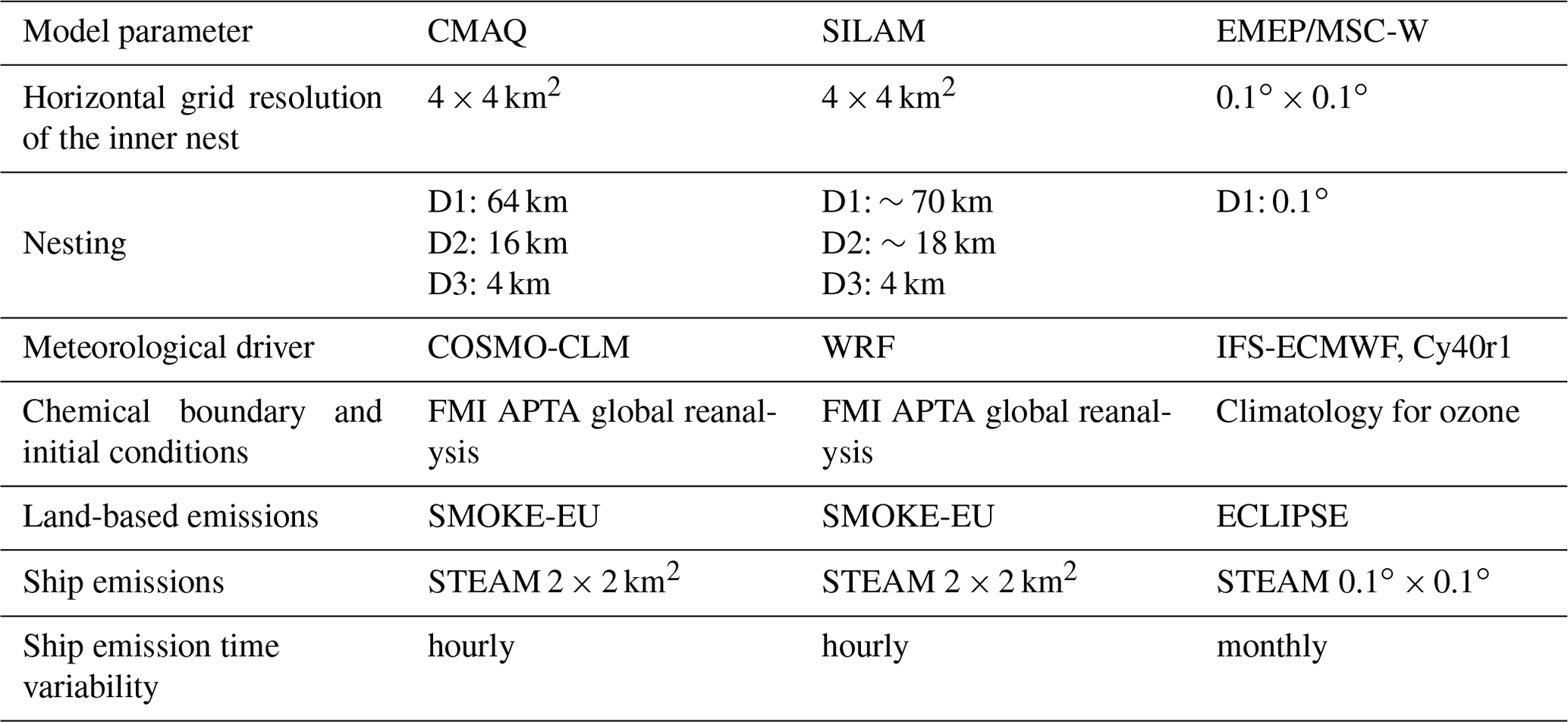
Nested simulations with CMAQ were performed with a coarse outer domain for the whole of Europe with a grid cell size of 64×64 km², an intermediate domain with 16×16 km² for northern Europe and an inner domain with a horizontal resolution of 4×4 km² for the entire Baltic Sea. Model results for the intercomparison were taken from the inner domain for the coastal regions and from the intermediate domain for parts of Sweden, Finland and the Baltic states. For details on the high-resolution output from CMAQ and an evaluation of the model set-up with a limited number of regional background stations, refer to Karl et al. (2019).

For the SILAM model, the grid cell size was roughly 70×70 km² for the outer domain, roughly 18×18 km² for the central domain and roughly 4×4 km² for the inner domain. The simulation time steps were 20, 10 and 4 min. Model results for the intercomparison were mostly from the inner domain, with parts of Finland and eastern Europe from the central domain. SILAM took part in AQMEII 1 and 3 intercomparisons showing comparable performance with other European state-of-the-art air quality models (Solazzo et al., 2012a, b, 2013, 2017; Vivanco et al., 2018; Marécal et al., 2015). The EMEP/MSC-W model was run with a 0.1×0.1^∘ resolution for the whole of Europe. A comprehensive description, including model evaluations, of the model results with the 0.1×0.1^∘ application of the EMEP model for 2013 can be found in Tsyro et al. (2015).

2.2.2 Meteorology

The SILAM model is run with meteorological input from a simulation with the Weather Research and Forecast (WRF) model v3.7.1 using original resolutions of 4.0, 16.0 and 64.0 km, for inner, central and outer domains, respectively. WRF was driven with large-scale meteorological forcing data taken from the ERA-Interim reanalysis (Dee et al., 2011). In general, linear interpolation was applied for the simulation, but conservation of mass was used where applicable. The high-resolution inner domain extended up to 2000 m in height and was therefore less influenced by upper-tropospheric dynamics of WRF. Kryza et al. (2017), using WRF in a similar configuration, evaluated the WRF meteorological fields against station observations in Poland. The 2 m air temperature (T₂) was underestimated in winter (bias smaller than −0.6 K), while temperature in the warm season was overestimated (bias up to +1.0 K). The largest errors for the 10 m wind speed (WS10) occurred in late summer and autumn and the largest errors for wind direction were in spring and summer. The error of wind direction was very small in winter. The spatial distribution of meteorological variables obtained from WRF were in close agreement with the station measurements, but the model performance was found to be worse for the seashore and mountain areas than for other inland areas (Kryza et al., 2017).

High-resolution meteorological fields for CMAQ were obtained from the COSMO-CLM (Rockel et al., 2008) model v5.0. The meteorological fields were converted to the extension, resolution and projection of the CMAQ nested grids, using an in-house modified version of MCIP. More details on the meteorological forcing data and the evaluation of precipitation can be found in Karl et al. (2019). Here we include an evaluation of T₂ and WS10 in the southern part of the Baltic Sea region. Temperature was compared against gridded observational dataset E-OBS v.16 (Cornes et al., 2018). Wind speed was compared against observational data from MiKlip DecReg of the German Weather Service (DWD). Monthly mean T₂ in Denmark and southern Sweden was underestimated in winter (bias smaller than −1.4 K) and overestimated in summer. The warm bias in summer was higher in Sweden (+1.4 K) than in Denmark (+0.4 K). The spatial correlation of T₂ in the southern Baltic Sea region based on 3 daily averages was remarkably good. Monthly mean WS10 was slightly overestimated in most parts of the region. The largest errors in wind speed occurred in Denmark and northern Poland during May and June.

EMEP/MSC-W was driven by meteorological data from the Integrated Forecasting System (IFS) of the ECMWF, version IFS38r2, with t1279 resolution (about 0.16^∘ resolution) interpolated to 0.1×0.1^∘. The ECMWF forecasting system of weather parameters is regularly validated by comparing them against European synoptic observation data available on the Global Telecommunication System (GTS). The evaluation of the weather forecast from cycle Cy40r1 is summarized as follows (Haiden et al., 2014). The frequency of light precipitation is overestimated with a bias of 1.2–1.4 mm d⁻¹ (for precipitation amounts >1 mm d⁻¹). T₂ has a negative night-time temperature bias over Europe in winter and early spring. For total cloudiness, bias and standard deviation are small in 2012. For WS10, the standard deviation is low and the night-time bias is very small.

The use of different meteorological datasets introduces additional variability which is, on one hand, wanted to achieve a wider range of possible results for estimating the effect of shipping on air quality but, on the other hand, complicates the interpretation of differences between the models.

2.2.3 Boundary conditions

The initial conditions (ICONs) for the simulation and the lateral boundary conditions (BCONs) for the outer European domain are taken from FMI APTA global reanalysis (Sofiev et al., 2018a). The global boundary conditions results have been interpolated in time and space to provide hourly boundary conditions for the respective outer domains of the CMAQ and SILAM simulations. The set-up for initial and boundary concentrations for EMEP/MSC-W is described in Simpson et al. (2012). ICONs and BCONs are based on long-term observations. For ozone, 3-D fields for the whole domain are specified from climatological ozone sonde datasets, modified monthly against clean-air surface observation. For most other chemical compounds they are defined by simple functions based on measurements and/or model calculations, prescribing concentrations in terms of latitude and time of year or time of day.

2.2.4 Anthropogenic land-based emissions

Anthropogenic land-based emissions at hourly resolution obtained from the SMOKE-EU (Bieser et al., 2011a) emission inventory were provided for CMAQ and SILAM. These emissions are based on officially reported EMEP emissions which are then distributed in time and space using appropriate surrogates like population density maps, street maps or land use maps. Point sources from the European point source emission register are considered. Vertical distribution of point source emissions is based on real-world stack information and calculated within SMOKE-EU (Bieser et al., 2011b). Dynamic emissions from agricultural activity and animal husbandry depending on meteorological variability are considered (Backes et al., 2016). The EMEP/MSC-W model uses anthropogenic emissions from the ECLIPSE gridded emission inventory (http://www.iiasa.ac.at/web/home/research/researchPrograms/air/ECLIPSEv5.html, last access: 17 April 2019). These emissions differ slightly from the reported national total EMEP emissions for 2012; see Wankmüller and Mareckova (2014). For the countries bordering the Baltic Sea (excluding Russia), the national total sulfur emissions from ECLIPSE are about 6 % higher and the NO₂ emissions about 10 % lower than the corresponding EMEP emissions.

2.2.5 Shipping emissions

The STEAM inventory for the Baltic Sea shipping emissions used in the SHEBA project consists of hourly updated 2×2 km² gridded data for NO_x, SO_x, carbon monoxide (CO) and particulate matter, which are further divided into elemental carbon, organic carbon, sulfate (${\mathrm{SO}}_{\mathrm{4}}^{\mathrm{2}-}$) and mineral ash. For the North Sea and other European seas the STEAM data for 2011 were used. Ship emissions were used with hourly time resolution in CMAQ and SILAM, whereas they were used with monthly resolution in EMEP/MSC-W. The use of monthly aggregated ship emissions in EMEP/MSC-W is justified by the fact that the same set of ship emissions from FMI is applied for different meteorological years in the routine application of EMEP modelling and that ship emissions from other seas were only available for 2011. Previous tests with daily and monthly aggregated ship emissions showed that the differences in results are very small. The use of North Sea ship emissions from 2011 on an hourly basis in CMAQ and SILAM causes some inconsistency because meteorological data from 2012 are used in the CTM simulations. Because we are mainly interested in the seasonal variability of pollutant concentrations based on daily averages, the outcome of this study will be less affected by the inconsistency between the timing of ship emissions and the meteorological conditions. STEAM emission data were provided for two vertical layers (below 36 m, from 36–100 m). In CMAQ and SILAM, emissions below 36 m were attributed to the vertical model layers below 42 m, while emissions above 36 m were attributed to the model layers between 42 and 84 m. In EMEP/MSC-W all ship emissions were attributed to the lowest vertical model layer, which typically has a height of 92 m.

2.3 Statistical analysis

2.3.1 Evaluation method for the total air pollutant concentrations

Model results for total surface concentrations of NO₂, O₃, SO₂ and PM_2.5 from the three CTMs are evaluated against available measurements of the air quality monitoring network from the AirBase v8 database (Simoens, 2014). AirBase is the air quality information system maintained by the European Environmental Agency (EEA) through the European topic centre on Air Pollution and Climate Change Mitigation. Table S1 in the Supplement gives a list of all rural and regional background monitoring stations. Concentrations of NO₂ are monitored at 17 stations, O₃ at 35, SO₂ at 11 and PM_2.5 at 8 rural and regional background stations. Table S2 gives all urban and suburban background monitoring stations included in the statistical evaluation of the models. Concentrations of NO₂, O₃, SO₂ and PM_2.5 are monitored at 52, 46, 37 and 10 stations of the urban background, respectively. Figure 2a shows locations of stations with NO₂ and with O₃ measurements. Figure 2b shows locations of the stations with SO₂ and with PM_2.5 measurements.

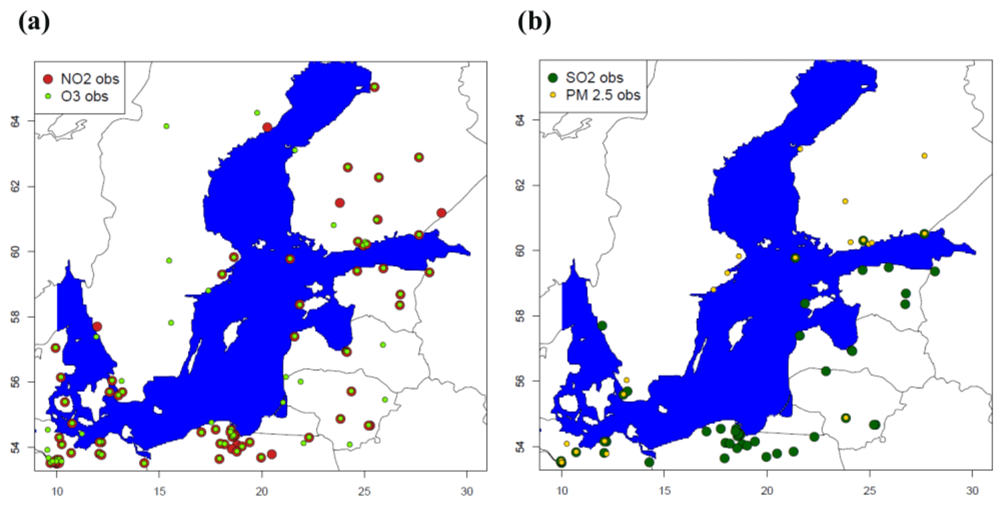
Figure 2 Map of the Baltic Sea region with the location of background monitoring stations used in the statistical performance analysis with observations of (a) NO₂ (filled red circles), O₃ (filled green circles), (b) SO₂ (filled dark green circles) and PM_2.5 (filled yellow circles). Same domain as in Fig. 1.

The model output of surface concentration fields of each CTM is used with its original horizontal resolution to calculate daily mean concentrations. The modelled concentrations are extracted from the respective model grid cell, where the selected monitoring stations are located. The evaluation was done for the entire year of 2012 based on daily means. The model output for PM_2.5 was taken from the modelled PM_2.5 containing aerosol water at 50 % relative humidity.

The performance of each model is quantified in terms of mean values (μ_Mod and μ_Obs), normalized mean bias (NMB), Spearman's correlation coefficient (R), root mean square error of the modelled values (RMSE) and fraction of model values within a factor of 2 of the observations (FAC2). Definitions of NMB, R, RMSE and FAC2 are given in Appendix A. The model performance analysis is discussed separately for rural background stations and urban background stations. In order to better highlight model differences in terms of urban areas and station types (i.e. rural, suburban, urban background sites), groups of stations (rural vs. urban) are generated in which statistical performance indicators are averaged. In the rural group, rural background and regional background stations are included, while in the urban group, urban background and suburban background stations are included. Monitoring stations classified as traffic stations and industrial stations were not included in the comparison, since the regional CTM systems applied here do not handle the local-scale dispersion near emission sources.

In the context of this evaluation of predicted air pollutant concentrations, we consider a correlation coefficient of more than 0.5 to indicate a correlation between modelled and observed time series, while values of 0.7 and above are considered to be good correlations. Hanna and Chang (2012) define certain acceptance criteria for model performance based on their experience in conducting a large number of model evaluation exercises. For rural stations, FAC2 values >0.5 and for urban stations FAC2 values >0.3 indicate acceptable performance. We adopt these bounds in the present study to characterize the predictive strength of the models with respect to the pollutant concentrations.

We compare the performance between models with the help of a graphical comparison in the form of box plots. Box plots of the correlation coefficient, NMB and RMSE, including either all rural or all urban monitoring stations, were prepared. The box plots show the median as a line dividing the box into two parts, the upper and lower quartiles as the ends of the box and the minimum and maximum values of the data and outliers.

In addition to the model performance for temporal correlation we evaluated the spatial correlation of the total air pollutant concentrations with the observations of the AirBase network for the three CTMs.

2.3.2 Significance of the ship contribution

The method described in Aulinger et al. (2016) was used to assess the significance of the ship influence on ambient NO₂ at the monitoring stations. The ship influence at a station was positively confirmed in the tests if (1) the concentrations increased and (2) the temporal correlation improved when shipping emissions were included in the CTM simulation.

By means of a paired t test it was first tested whether the modelled NO₂ concentrations at the monitoring stations with available NO₂ observations (Table S1) significantly increased if shipping emissions were considered. This test estimated whether the mean concentration difference between the noship run and the base run (noship – base) is significantly equal to or greater than zero, indicated by the probability p_bias. If the value of p_bias was greater than the level of significance of 0.05, then this hypothesis was confirmed, which means that no difference between the base run and the noship run could be statistically proven. In case p_bias was less than 0.05, it was decided that the model run without shipping emissions led to lower concentrations, confirming the ship influence.

The significance of the improvement in the correlation between simulations and observations was tested by calculating the Fisher z transformation of the two correlation coefficients for the two model runs (noship and base) and testing the hypothesis “greater than”. Correlation coefficients were calculated with Spearman's method (Myers and Sirois, 2006) for consistency with the statistical evaluation. The probability p_corr was calculated for the hypothesis that the correlation between the base run and observations is greater than the correlation between the noship run and observations. We accepted this hypothesis if the probability was higher than 0.9. Therefore, in the following, a station i with $p_{\text{corr},i}>\mathrm{0.9}$ for a specific CTM simulation is termed “ship influenced”.

3 Results

3.1 Statistical evaluation of air pollutant concentrations

3.1.1 Rural vs. urban sites

A statistical performance analysis for each of the three CTMs was undertaken using the available observation data form AirBase for 2012 based on daily mean total concentrations. The evaluation results for the temporal variation of air pollutants are summarized in Table S3 for daily mean NO₂, in Table S4 for daily mean O₃, in Table S5 for daily mean SO₂ and in Table S6 for daily mean PM_2.5. In the following, the performances of the models that simulate air pollutant concentrations are compared and discussed separately for the group of rural stations and for the group of urban stations in order to highlight differences in the predictive capability of the models for rural vs. urban sites.

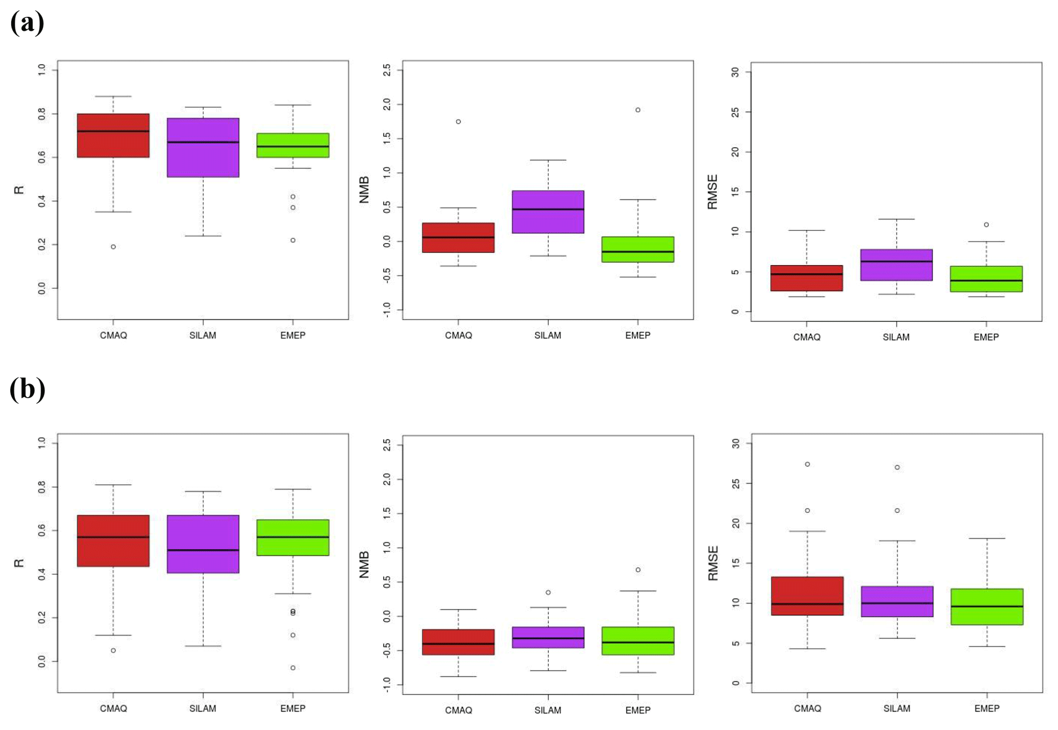
Figure 3 Comparison of statistical indicators for NO₂ daily means (in the order R, NMB and RMSE) between three CTMs at (a) rural background stations and (b) urban background stations. Outliers shown as small circles.

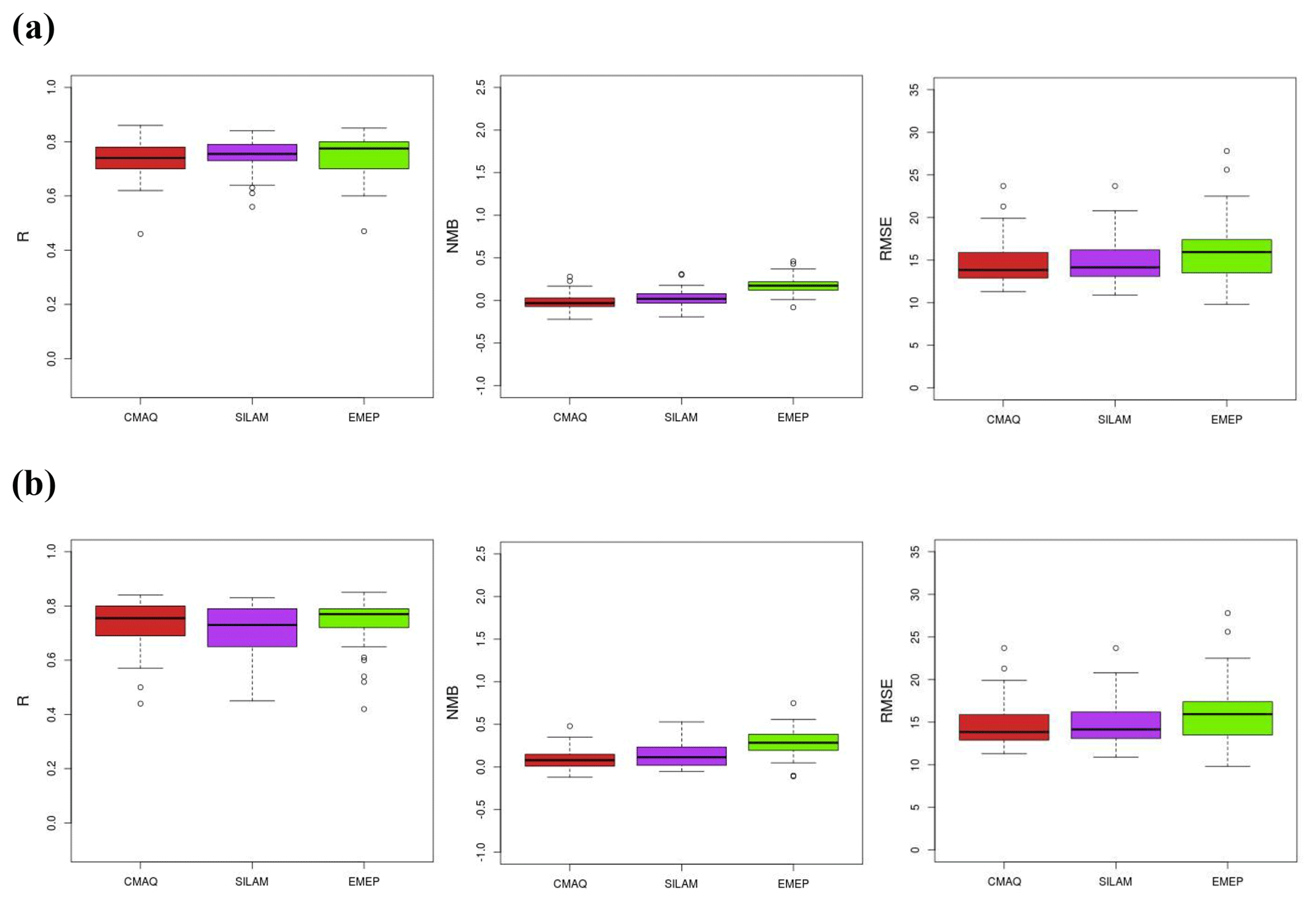
Figure 4 Comparison of statistical indicators for O₃ daily means (in the order R, NMB and RMSE) between three CTMs at (a) rural background stations and (b) urban background stations. Outliers shown as small circles.

The atmospheric lifetime of NO₂ is relatively short: a few hours in summer and up to 1 day in winter (Schaub et al., 2007); hence differences between rural and urban sites are expected due to the higher emission density in urban or industrial areas. The urban station average of observed annual mean NO₂ is more than twice the concentration average at rural sites. The three CTMs underestimate the annual means at the urban sites. The overall correlation of NO₂ for rural stations is good for all models. The overall correlation of NO₂ for urban sites is lower than at the rural sites (Fig. 3). At most urban stations, models underestimate the observed daily mean NO₂ by ca. 40 % (Table S3). The general underestimation of NO₂ at urban sites has been evident in other multi-model air quality studies in Europe (e.g. Giordano et al., 2015). The finer horizontal resolution of CMAQ and SILAM (4 km) compared to EMEP/MSC-W (11 km) does not result in a significant improvement in the urban bias and urban temporal correlation. This result was expected based on the study by Schaap et al. (2015), who found no further improvement in the urban signal, i.e. the concentration difference between high-emission areas and their surroundings, when increasing the resolution from 14 to 7 km in the same model. Moreover, increasing the spatial resolution in the model does not help to significantly improve the performance in time because the temporal variability of pollutants is affected by the meteorological conditions and pollution levels upwind (Schaap et al., 2015).

Figure 5 Comparison of statistical indicators for SO₂ daily means (in the order R, NMB and RMSE) between three CTMs at (a) rural background stations and (b) urban background stations. Outliers shown as small circles.

Tropospheric ozone is largely controlled by the atmospheric transport from regions outside the study area, by stratosphere–troposphere exchange and by the photochemical production through the oxidation of VOCs and carbon monoxide (CO) in the presence of NO_x and sunlight. The higher density of NO_x emissions in urban areas is expected to lead to a larger titration effect of NO on ozone, which results in lower average O₃ at the urban sites compared to rural sites. The models slightly overestimate the O₃ measurements at urban sites, with CMAQ having the smallest bias. CMAQ and SILAM predict similar annual mean concentrations as observed for both rural and urban sites, whereas EMEP/MSC-W predicts higher annual mean ozone (Fig. 4). The ozone bias might be linked to boundary conditions (Giordano et al., 2015): the EMEP model uses ozone boundary conditions from long-term observations, whereas CMAQ and SILAM models use boundary conditions from the FMI APTA global reanalysis. The models slightly overestimate the O₃ measurements at urban sites, with CMAQ having the smallest bias (average NMB =0.08). The average RMSE values for the rural sites and the urban sites are similar for the three models (Fig. 4), indicating comparable model performance for the CTMs with respect to daily mean O₃ concentrations.

Figure 6 Comparison of statistical indicators for PM_2.5 daily means (in the order R, NMB and RMSE) between three CTMs at (a) rural background stations and (b) urban background stations. Outliers shown as small circles.

Another major air pollutant is SO₂. It is primarily emitted from anthropogenic emission sources such as coal power plants, residential heating, waste incineration and shipping activities. SO₂ acts as a precursor to sulfates, which are one of the main components of particulate matter in the atmosphere. The atmospheric lifetime of SO₂ is on the order of a few days (Lee et al., 2011). SO₂ can still be considered to be relatively short-lived and thus less influenced by transport from regions outside the study area. Most emission sources of SO₂ are located in urban areas. In the case of power plants, the emissions of SO₂ are, however, injected at elevated height and therefore do not directly impact the surface concentrations in the urban area. The urban station average of observed annual mean SO₂ is 3 times higher than at the rural stations. At rural and urban sites, the modelled daily mean SO₂ from CMAQ and SILAM has a positive bias, whereas the modelled daily mean SO₂ from EMEP/MSC-W has a slight negative bias (Fig. 5). For EMEP/MSC-W some urban stations have a FAC2 below 0.3 due to the underestimation of observed SO₂. At urban stations, the temporal correlation between model data and observed SO₂ shows a mixed performance by the models, with good correlation at some stations and poor correlation at others. The model data and the observations for daily mean SO₂ at the rural sites are correlated, but with only 10 stations, the rural station group for SO₂ is rather small, limiting the conclusions that can be drawn from the statistical analysis. The weaker performance of the models for SO₂ at the rural sites is related to uncertainties in local residential heating emissions, as the timing of use and the sulfur content of burned fuels are difficult to predict.

Ambient PM_2.5 is a widespread pollutant, which is directly emitted by biomass and fossil fuel combustion in domestic and industrial activities, and it is also formed from gaseous precursors such as NO_x, SO₂, NH₃ and NMVOC in the atmosphere. The atmospheric lifetime of PM_2.5 is on the order of days or weeks and thus PM_2.5 can be subject to long-range transport. For PM_2.5, smaller differences between rural and urban stations are expected than for NO₂ and SO₂ because PM_2.5 has a large secondary component, which is generally more homogeneously distributed over rural and urban areas. SILAM is able to reproduce annual mean PM_2.5 concentrations for urban stations, whereas CMAQ and EMEP/MSC-W give lower annual mean values than observed. For urban stations, the temporal correlation of daily mean PM_2.5 is good for all models, whereas for rural stations the temporal correlation is slightly better for EMEP/MSC-W than for CMAQ and SILAM (Fig. 6). At both rural and urban sites, the modelled daily mean PM_2.5 from CMAQ and EMEP/MSC-W has a slightly negative bias, whereas modelled daily mean PM_2.5 from SILAM has no bias.

3.1.2 Spatial correlation

The spatial correlation between modelled and observed annual mean total pollutant concentrations for the three CTMs is presented in Fig. 7. Because NO_x is mainly emitted near the ground, the spatial distribution of NO₂ is expected to be highly correlated with emissions. The improvement in spatial resolution of emissions should lead to improved spatial correlation between modelled and observed concentrations. In contrast with this expectation, EMEP/MSC-W shows the best correlation and the lowest bias. Observed annual mean NO₂ at urban stations is strongly underestimated by SILAM and in CMAQ. The positive bias indicates that observed NO₂ at rural stations tends to be overestimated by these two models. The annual mean O₃ is closely linked to the annual mean NO₂ through the local titration effect. Hence, lower than observed O₃ at rural stations for SILAM and CMAQ is related to the higher than observed NO₂. The models are capable of representing the seasonal variation of ozone, with highest average concentrations in spring, followed by summer, and lowest concentrations in winter and autumn.

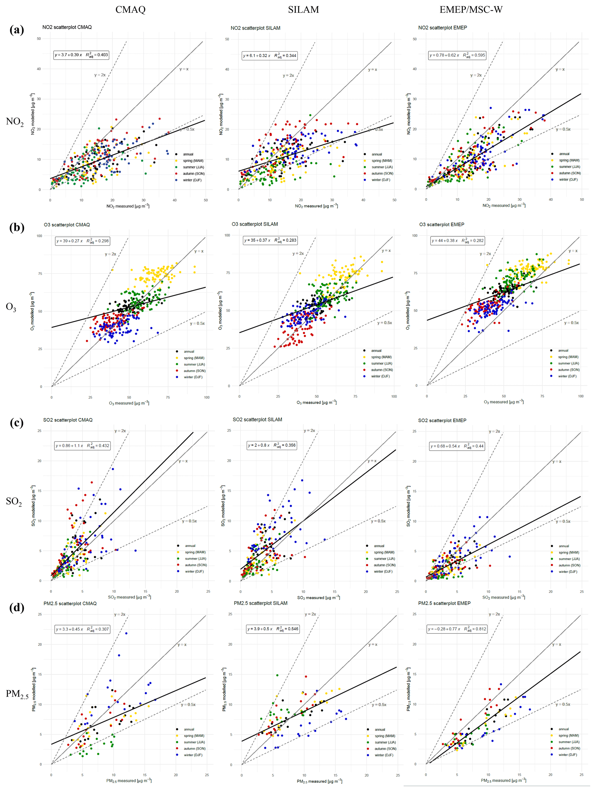
Figure 7 Spatial correlation of annual mean concentrations (µg m⁻³) and the seasonal averages from CMAQ (left column), SILAM (middle column) and EMEP (right column) in the Baltic Sea region for (a) O₃, (b) NO₂, (c) SO₂ and (d) PM_2.5.

The spatial correlation between modelled and observed SO₂ is weaker than that for NO₂, which is probably due to the fact that most SO₂ sources are emitting into higher vertical layers. CMAQ and SILAM overestimate SO₂ in autumn and winter at many stations by a factor of 2 or more, which is likely related to the uncertainty in the residential heating emissions. EMEP/MSC-W underestimates SO₂ in summer, which might be connected to uncertainties in the vertical emission distribution. EMEP-MSC/W shows the best spatial correlation for PM_2.5 with almost no bias. However, annual average PM_2.5 is underestimated by 23 % on average. For CMAQ and SILAM the spatial correlation for annual mean PM_2.5 has a positive bias due to overestimation at the rural stations. At almost all stations, CMAQ underestimates PM_2.5 in summer. This has also been evident for regional background stations of the EMEP monitoring network and can partly be attributed to the underestimation of secondary organic aerosols in the CMAQ simulation (Karl et al., 2019). SILAM underestimates PM_2.5 in winter. Since PM_2.5 in winter is mainly from anthropogenic sources and SILAM uses the same emissions as CMAQ, the discrepancy in winter PM_2.5 is attributed to problems with simulating stagnant meteorological conditions.

3.2 Evaluation of ship-related concentration contributions

A direct comparison of the modelled ship-related concentration contribution to measurements of the shipping signal (in exceedance of the background air) is hampered by the fact that measured concentration increases due to individual ship plumes do not reflect the entire contribution of shipping at sea. In order to evaluate the modelled ship contributions, a statistical method (Sect. 2.3.2) was applied to decide whether the modelled concentration as well as the correlation with observed daily mean NO₂ concentration at a specific station increases significantly when ship emissions are included in the CTM simulation. The results of the significance test are summarized in Table S7.

A significant concentration increase was found at all 69 stations for the three CTMs. However, the significance of the concentration increase only shows that the modelled concentrations at a station are sensitive to ship emissions. The correlation increases significantly (on 0.9 or 0.95 level) at 10, 7 and 8 stations for CMAQ, SILAM and EMEP/MSC-W, respectively (Table S7).

Four ship-influenced stations were identified by all models: Vilsandi (EE0011R, Estonia), Utö (FI00349, Finland) at the shoreline, Norr Malma (SE0066A), 20 km inland at the east coast of Sweden and Lübeck-St Jürgen, (DESH023, Germany) close to a port (time series plots in Appendix B). At Norr Malma, NO₂ is largely overestimated by the models in summer when ship emissions are included. We suggest that, due to the high spatial resolution of the model, ship exhaust plumes are resolved but not adequately dispersed in the models. Since the models do not specifically treat the plume dispersion of individual ships, the spreading of the plume might not be sufficiently large or the plume height from ship exhausts is not properly considered with the applied vertical profile of ship emissions.

Ship-influenced stations found by any of the models included shoreline stations (Virolahti, FI00351, Finland; Lahemaa, EE0009R, Estonia), stations in harbour cities (Rostock Warnemünde, DEMV021, Germany; Kiel, DESH033, Germany; Aalborg/8158, DK0053A, Denmark, Södermalm, SE0022A, Sweden; Gdansk Pm.a09aN, PL0053A; Poland) and one urban inland station (Pm.63.wDSAa, PL0171A, Poland). The corresponding time series plots of daily mean NO₂ are shown in Appendix B. Observed daily mean NO₂ at the two urban stations in Poland is underestimated by all models, indicating missing local emissions from other sectors. The ship influence at station Rostock Warnemünde, located close to a harbour, was significant in EMEP/MSC-W but not in the other two models (Fig. B1i). This could indicate that differences in the meteorological data, in particular wind flow fields, are responsible for the different ship influences. Although, the timing and location of ship exhaust plumes – based on AIS data – should be accurate during the port stays, the emission fluxes at berth are more challenging to estimate, because this involves an estimation of electrical power usage during the port stays. Evaluation of the ship contribution in Rostock using an urban air quality model with a high degree of detail on ship emissions and other urban emissions showed that shipping significantly impacts on annual averaged NO₂ in the city domain (Ramacher et al., 2019).

For all ship-influenced stations, time series plots of daily mean O₃ are compiled in Fig. S1 in the Supplement. Including the shipping emissions in the model simulations affected ozone concentrations mainly in the summer months. The change in modelled O₃ due to shipping was below 6 % on average in summer at the ship-influenced stations. At most of the stations, including ship emissions increased the modelled O₃ concentration as a consequence of photochemical ozone production. The seasonal variation of NO₂ at the ship-influenced sites with peak concentrations in winter is in general reproduced by the models. Including ship emissions improved the agreement between modelled and measured NO₂ daily mean concentrations at about 50 % of the stations. For more than 70 % of all stations the observations of total NO₂ concentrations are reproduced by the models within a NMB range from −0.5 to 0.5 in the base simulation (Fig. S2).

3.3 Comparison of the spatial distribution of air quality indicators

3.3.1 Spatial distribution of annual mean NO₂

A strong south–north gradient for annual mean NO₂ concentrations is found for the Baltic Sea region in the three base simulations, with 4–5 times higher NO₂ concentrations in the southwestern part than in the northern part of the region (Fig. 8a). High modelled NO₂ concentrations are predicted in Denmark, northern Germany and Poland as well as over the Danish Straits and in the urbanized areas of the region. Modelled annual mean NO₂ concentrations in the proximity of the main shipping routes several times exceed the concentrations in the regional background. EMEP/MSC-W shows the strongest concentration gradients between urban and rural areas and between shipping lanes and the surrounding sea. The simulations with the other two models result in a wider spread of the NO_x emissions from the shipping routes and the urban centres, indicating stronger horizontal transport by advection and diffusion in CMAQ and SILAM. This finding is counterintuitive as the NO_x emissions are initially less diluted than in the EMEP/MSC-W simulation because of the smaller volume of the grid boxes and therefore result in higher NO_x concentrations near the emission sources. Atmospheric transport by diffusion processes are subgrid mixing processes, which are not resolved by the given resolution of the applied models. For large grid cells, e.g. 50×50 km², the numerical diffusion will usually be much larger than the physical diffusion in the horizontal direction. However, at finer-resolution scales, the physical diffusion will gradually become more important than numerical diffusion and becomes greater than numerical diffusion for a cell size of 5×5 km² or below (Karl et al., 2014). The wider spread of elevated NO₂ concentrations is also indicative of a longer atmospheric lifetime of NO₂ in CMAQ and SILAM compared to the simulation with EMEP/MSC-W. NO₂ is removed relatively quickly in the lower troposphere through the reaction with hydroxyl (OH) radicals to form HNO₃. The rate coefficient for this reaction, k(NO₂+OH), is similar in the three models ((1.1–1.2)$\times {\mathrm{10}}^{-\mathrm{11}}$ cm³ s⁻¹ at 298 K). Thus, differences in the NO₂ lifetime are mainly due to different abundances of OH radicals in the simulations. High NO₂ concentrations in Belarus and Russia in the SILAM simulation are an artefact from merging with the output of the coarser central model grid (Sect. 2.2.1).

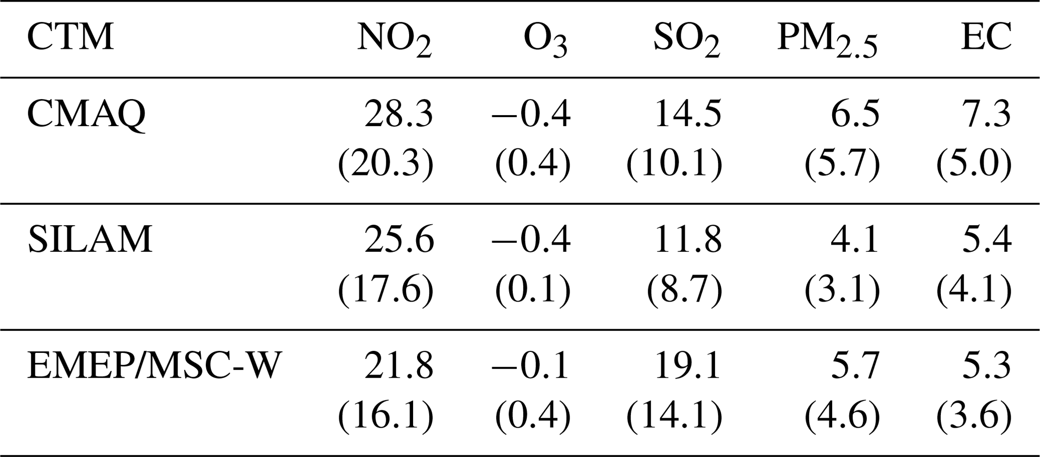
Table 2 Spatial averages of the annual mean concentrations of NO₂, O₃, SO₂, PM_2.5 and EC in µg m⁻³ for the study domain (Baltic Sea region as in Fig. 1).

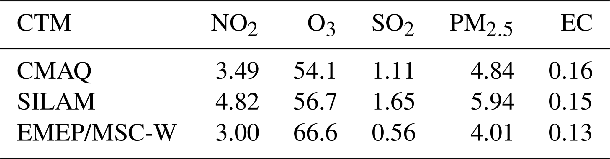
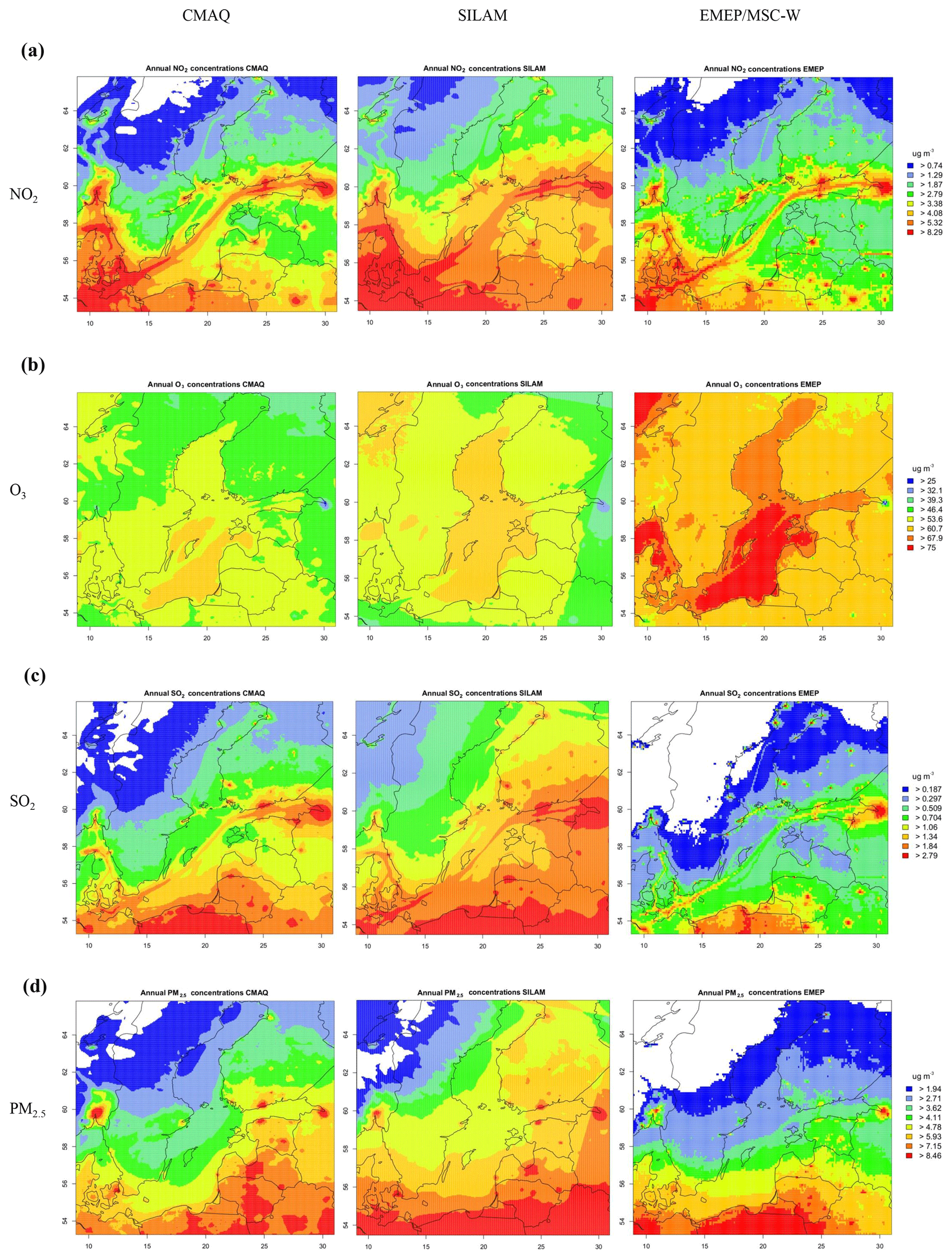
Figure 8 Comparison of the spatial distribution of annual mean concentrations (µg m⁻³) from CMAQ (left column), SILAM (middle column) and EMEP (right column) in the Baltic Sea region for (a) O₃, (b)  NO₂, (c) SO₂ and (d) PM_2.5. Empty areas correspond to concentrations between zero and the lowest value in the legend.

3.3.2 Spatial distribution of annual mean O₃

Modelled annual mean O₃ concentrations over the Baltic Sea are 15 %–25 % higher than over land but are reduced along the shipping lanes due to the titration effect caused by the ship-emitted NO_x (Fig. 8b). Lowest ozone concentrations are seen for St Petersburg (< 32 µg m⁻³) in the three simulations, although we note that the city is outside of the high-resolution grid in the case of SILAM. The spatial average of annual mean O₃ is clearly higher for the EMEP/MSC-W simulation, by ca. 20 % compared to the other two simulations (Table 2). The most probable reason for the difference is the application of different sets of boundary conditions for the European model domains, as discussed in Sect. 3.1.1. Model simulations for Europe have shown a high sensitivity of ozone changes to the dry deposition to vegetation (Andersson and Engardt, 2010). Thus differences in the deposition schemes may partly explain the different O₃ levels over the continent, e.g. when comparing ozone over Sweden and Finland between CMAQ and SILAM.

3.3.3 Spatial distribution of annual mean SO₂

Clear differences in the spatial distribution of the annual mean SO₂ concentrations are found between CMAQ and SILAM on one hand and EMEP/MSC-W on the other hand (Fig. 8c). The simulation with CMAQ and SILAM shows a southeast–northwest gradient with elevated SO₂ over large parts of the southern Baltic Sea region, Poland, Belarus, Russia and the Baltic States with annual mean concentrations in the range of 1.3–3.0 µg m⁻³. Residential heating emissions and power plant emissions for district heating in the urban centres and rural areas strongly contribute to the high SO₂ concentrations in this subregion. In the EMEP/MSC-W simulation, elevated SO₂ concentrations are present along the main shipping routes in urban areas and in Poland, whereas the levels of SO₂ outside of these areas are much lower. The concentration gradients between urban and rural areas and between shipping lanes and surrounding sea are up to 2.5 µg m⁻³ for EMEP/MSC-W, while it is only up to 0.7 µg m⁻³ for CMAQ and SILAM. Factors contributing to the different gradients are differences in the representation of horizontal transport (see Sect. 3.3.1), differences in the meteorological conditions and differences in the atmospheric lifetime of SO₂. The atmospheric lifetime of SO₂ is determined by its reaction with the OH radical and by its removal via dry deposition. In EMEP/MSC-W, the canopy uptake of SO₂ is strongly controlled by NH₃ levels, and the implemented deposition parameterization accounts for co-deposition effects on the dry deposition of SO₂ (Simpson et al., 2012). Co-deposition effects are not considered in the other two models.

3.3.4 Spatial distribution of annual mean PM_2.5

Modelled annual mean PM_2.5 is higher in the southern part, both over land and sea, than in the northern part of the Baltic Sea region (Fig. 8d). On annual average, PM_2.5 concentrations are not elevated along the shipping routes. The seasonal differences between summer and winter will be discussed below (Sect. 3.5) and will help to understand differences between the models. High PM_2.5 levels (8 µg m⁻³ and higher) are simulated in the urban areas of major cities like Copenhagen, Oslo, Helsinki, Riga, Tallinn and St Petersburg. The high PM_2.5 levels over the continent in the southern part of the Baltic Sea region presumably result from a combination of land-based primary emissions, long-range transported particles and the formation of secondary particulate matter.

Table 3 Relative ship contribution to the spatial average of annual mean NO₂, O₃, SO₂, PM_2.5 and EC in percent for the study domain (Baltic Sea region as in Fig. 1). Values in brackets denote the average relative ship contribution in the coastal land areas of the domain.

3.3.5 Recommendations from the comparison between the CTM systems

The applied CTM modelling systems originate from different institutes and represent independent lines of development. Their operations require varying degrees of the user experience, input data requirements and computational demand. All three systems are open source, installed and used in a number of countries and possess long records of operational and research applications. The EMEP and SILAM models are usually less demanding than CMAQ in terms of computational resources and input data. Yearly totals of anthropogenic emissions can be used as input to the two models, which perform the temporal disaggregation of emissions in line with the computation. CMAQ probably has the most-extensive user community with support provided by the developers from the US Environmental Protection Agency (Otte and Pleim, 2010).

Comparison of the model performances does not give an unequivocal answer: all model skills are within the uncertainty in the corresponding parameters (Figs. 3–6). One should, however, bear in mind that the EMEP model was run with a lower resolution than two other models. There are certain systematic differences between model results from SILAM and CMAQ on one hand and EMEP on the other: e.g. higher NO₂ concentrations at rural stations and lower at urban stations (compare the spatial correlation of annual station averages in Fig. 7). To a large part, this mismatch can be attributed to the spatial distribution of anthropogenic emissions in the SMOKE inventory, applied in the two CTM systems in comparison with ECLIPSE emissions used by EMEP.

The EMEP/MSC-W model is routinely used for multi-year calculations, facilitating its use for the HELCOM (Baltic Marine Environment Protection Commission – Helsinki Commission) evaluation of trends in the deposition of nitrogen and sulfur in the Baltic Sea region. CMAQ is being used for a variety of environmental modelling problems including regulatory applications and evaluation of emission control strategies (Otte and Pleim, 2010). CMAQ is continuously updated to remain a state-of-the-art regional CTM. A specific advantage of SILAM is the online computation of wildfire emissions and operational input of hourly STEAM ship emissions. The evaluation of modelled daily mean PM_2.5 showed that RMSE station values for SILAM are within a smaller range (between lower and upper quartiles) than the other two models (Fig. 6). The model was also recently applied to 35-year-long global-to-local reanalysis of air quality by Kukkonen et al. (2018). SILAM can therefore be recommended for use in advanced research applications, specifically addressing the abundance and composition of particulate matter.

3.4 Comparison of the ship contribution in the three CTMs

The influence of shipping emissions on the air quality was evaluated for the annual mean concentrations of the three CTMs. The results for the impact of shipping emissions were calculated as differences between the base and the noship simulations. Results for the absolute ship-related concentrations of O₃, NO₂, SO₂ and PM_2.5 are shown in Fig. 9, the resulting relative ship contribution to annual mean concentrations is shown in Fig. S3 and the spatial average of the relative ship contribution is given in Table 3.

3.4.1 Ship contribution to annual mean NO₂

The ship-related annual mean NO₂ concentrations from the three CTMs are in the range of 3–5 µg m⁻³ along the main shipping routes. The NO₂ ship contribution decreases to Baltic Sea background values (about 1 µg m⁻³) within a few hundred kilometres from the centre of the shipping routes. Ships emit NO_x mainly in the form of NO, which is, however, quickly converted to NO₂. Thus atmospheric NO_x is mainly in the form of NO₂. The relative contribution of ship emissions to annual mean NO₂ is more than 40 % over the Baltic Sea (Fig. S3), 22 %–28 % for the entire Baltic Sea region and 16 %–20 % in the coastal land areas (Table 3). In particular, NO_x emissions from shipping affect the harbour cities of the region and coastal areas in southern Sweden. Local differences between the models might be due to the different meteorological drivers or differences in the titration efficiency for ozone.

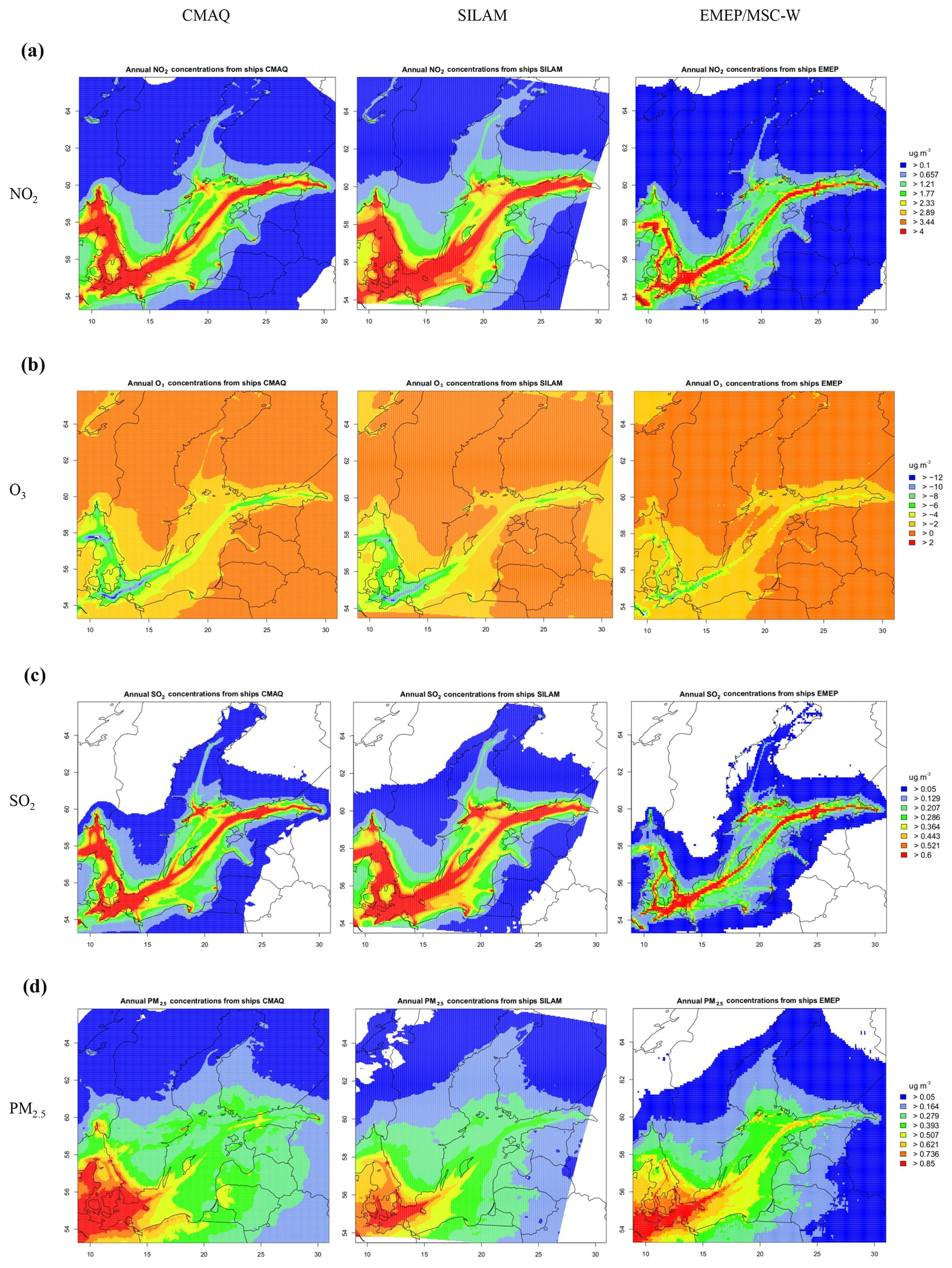
Figure 9 Comparison of the spatial distribution of annual mean ship-related concentrations (absolute ship contributions in µg m⁻³) of the CMAQ (left column), SILAM (middle column) and EMEP (right column) models in the Baltic Sea region for (a) O₃, (b) NO₂, (c) SO₂ and (d) PM_2.5.

3.4.2 Ship contribution to annual mean O₃

In the proximity of the main shipping routes, negative concentration differences for the modelled annual mean O₃ between the base and the noship simulation are obtained as a result of the titration effect by the NO_x emissions from shipping. The highest ozone reduction due to shipping is found in the western part of the Baltic Sea. In the CMAQ simulation the depletion of ozone is stronger than in the other two models, with O₃ reduction of 6–12 µg m⁻³ in the Kattegat and in the Danish Straits. The hourly variation of ship emissions is represented in the simulations with CMAQ and SILAM, whereas monthly averaged ship emissions are used in the EMEP/MSC-W simulation. Emission peaks of NO_x from ships that are present in the hourly data can result in occasional stronger ozone titration, leading to overall higher reduction of ozone than is the case for monthly averaged ship emissions. Over the coastal land areas, the average impact on annual mean of O₃ is very small, with ozone increases between 0.1 % and 0.4 % for the models.

3.4.3 Ship contribution to annual mean SO₂

Ship emissions of SO₂ have a high contribution to annual mean SO₂ concentrations over the Baltic Sea. The ship contribution to SO₂ is 0.5–0.7 µg m⁻³ in a wide corridor around the main shipping routes of the Baltic Sea. While the absolute ship contribution of the three CTMs is similar, the relative ship contribution in the EMEP/MSC-W simulation is higher in most areas of the Baltic Sea and in Sweden, because the background atmospheric SO₂ levels in this simulation are lower than in CMAQ and SILAM.

3.4.4 Ship contribution to annual mean PM_2.5

The ship contribution to annual mean PM_2.5 shows a gradient from southwest to north with highest concentrations over Denmark, the west coast of Sweden, the Belt Sea/Kattegat and over the sea south of Sweden, with maximum values up to 0.9 µg m⁻³. The relative contribution in these ship-impacted areas is up to 10 %. The average ship contribution for the three CTMs is in the range of 4.1 %–6.5 % in the entire Baltic Sea region and 3.1 %–5.7 % in the coastal land areas. The absolute ship contribution in SILAM is slightly smaller than for the other two models, in particular in the southwestern part of the Baltic Sea region (Fig. 9d). The ship-related PM_2.5 affects the coastal areas in the Baltic Sea region, as its influence extends further inland than is the case for ship-related NO₂ or SO₂. This can be attributed to the formation of secondary particulate matter in the ship exhaust plume during its transport away from the main shipping routes.

3.5 Comparison of PM_2.5 in summer and autumn

CMAQ and EMEP/MSC-W simulations predict higher seasonal mean concentrations of PM_2.5 in autumn (average of September, October and November, SON) than in summer (average of June, July and August, JJA), whereas the SILAM simulation predicts higher PM_2.5 in summer (Fig. 10a, c; Table S10). The temporal correlation between model data and observations of daily mean PM_2.5 for the average of the AirBase stations is slightly better in autumn than in summer (Tables S8 and S9). Observed PM_2.5 in summer is underestimated strongly by CMAQ (at almost all stations; see Sect. 3.1.2) and to some extent by EMEP/MSC-W. In autumn all models are in better agreement with observed PM_2.5.

The SOA formation mechanism in the applied version of CMAQ (i.e. v5.0.1) is probably not adequate for reproducing the summertime aerosol. Primary organic aerosol (POA), SOA and organic vapours in the atmosphere should be considered a dynamic system that constantly evolves due to multigeneration oxidation (Robinson et al., 2007). We note that multigenerational ageing chemistry for the semi-volatile POA was introduced in CMAQ v5.2, based on the approach by Donahue et al. (2012), which considers the functionalization and fragmentation of organic vapours upon oxidation. In addition, wildfire emissions have not been considered in the simulation with CMAQ. Wildfires emit large quantities of organic material and are associated with high biogenic VOC emissions due to high temperatures, leading to increased SOA formation (Lee et al., 2008).

In summer, modelled mean PM_2.5 in the region is much higher in the SILAM simulation (5–8 µg m⁻³ in most parts, 7.4 µg m⁻³ on regional average, 5.4 µg m⁻³ on average in coastal land areas) than for the other two models (<4 µg m⁻³, except for the urban areas). The higher summertime PM_2.5 in SILAM is most likely due to more efficient SOA production and primary emission from wildfires and/or mineral dust. A previous comparison of the models to PM_2.5 observations from the EMEP station network in Europe reported similar seasonal mean concentrations of the SIA components, i.e. nitrate (${\mathrm{NO}}_{\mathrm{3}}^{-}$), ammonium (${\mathrm{NH}}_{\mathrm{4}}^{+}$) and ${\mathrm{SO}}_{\mathrm{4}}^{\mathrm{2}-}$, for the three CTMs in summer (Prank et al., 2016).

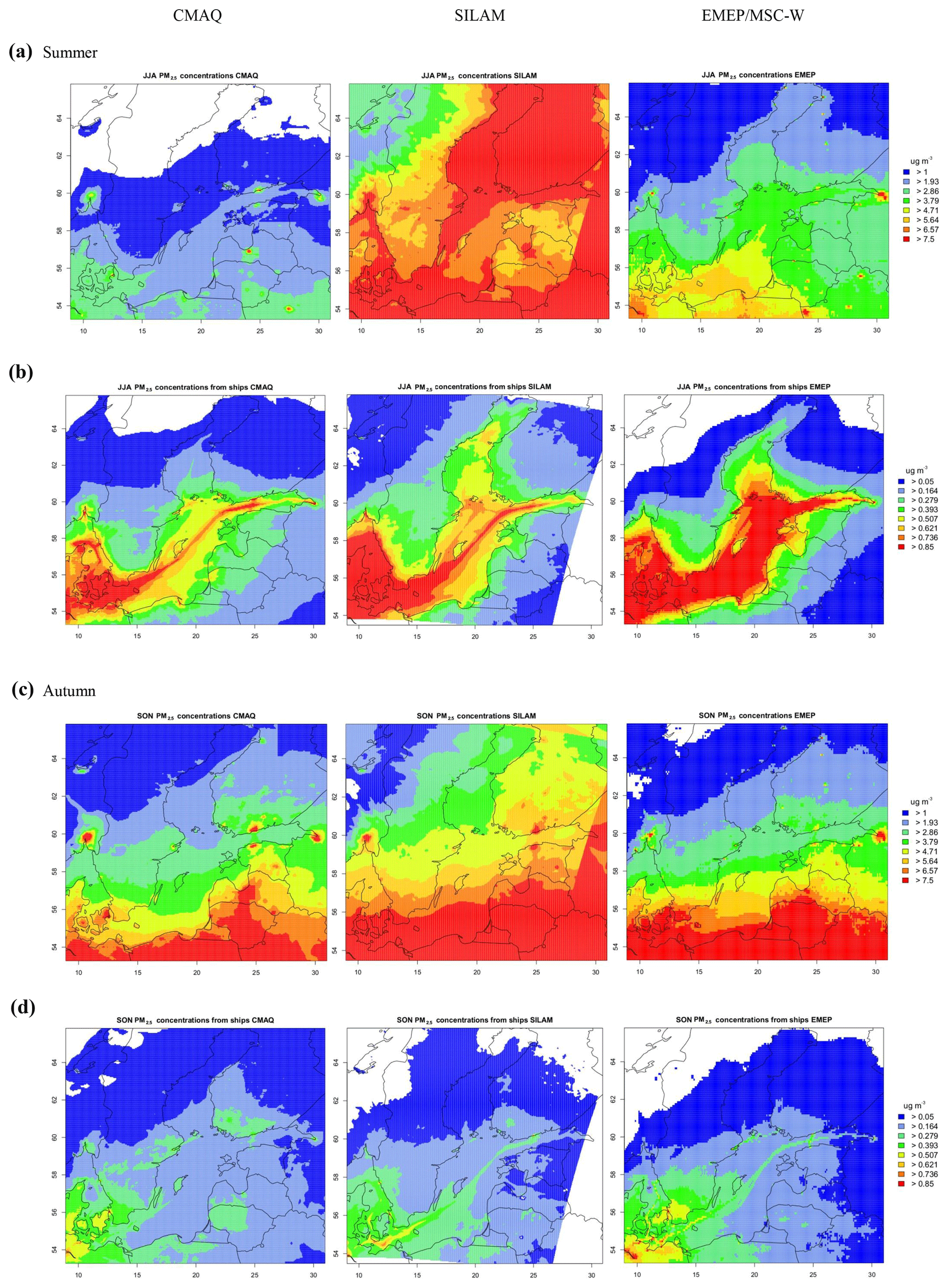
Figure 10 Comparison of PM_2.5 in summer and autumn from CMAQ (left column), SILAM (middle column) and EMEP (right column) in the Baltic Sea region for (a) JJA mean concentration (µg m⁻³), (b) JJA mean ship contribution (µg m⁻³), (c) SON mean concentration and (d) SON mean ship contribution. Empty areas correspond to concentrations between zero and the lowest value in the legend.

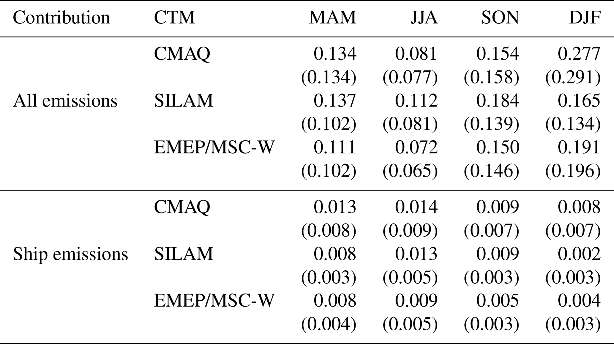
Table 4 Spatial averages of seasonal mean concentrations of EC (µg m⁻³) from the base simulation and ship contributions to EC levels (µg m⁻³) for the study domain (Baltic Sea region as in Fig. 1). Mean values are given for spring (March to May; MAM), summer (JJA), autumn (September to November; SON) and winter (January, February and December 2012; DJF). Values in brackets denote the seasonal mean concentrations in the coastal land areas of the domain.

The calculated ship contribution from all models is higher in summer than in autumn (Table S10). The simulations reflect the greater importance of shipping activities during summer and their influence on PM_2.5 levels over the entire Baltic Sea and the coastal areas (Fig. 10b). In particular Denmark and the Swedish west coast is highly impacted in summer, with a ship contribution of 0.5–0.9 µg m⁻³ to ambient PM_2.5 levels.

In autumn, all CTMs predict high levels of PM_2.5 in the southern part of the Baltic Sea region, exceeding 6 µg m⁻³. High PM_2.5 in autumn is typically attributed to stagnant meteorological conditions and higher emissions of primary particulate matter from residential heating and energy production. Modelled PM_2.5 in Sweden and Finland is higher in SILAM than in the other two models. SILAM overestimates observed PM_2.5 at the stations in Sweden, Lithuania and Finland in summer (NMB: 0.54 on average) and autumn (NMB: 0.31 on average). In an earlier model comparison, all three models were shown to overestimate ${\mathrm{NO}}_{\mathrm{3}}^{-}$ and ${\mathrm{NH}}_{\mathrm{4}}^{+}$ in autumn, while SILAM also overestimated ${\mathrm{SO}}_{\mathrm{4}}^{\mathrm{2}-}$ in autumn (Prank et al., 2016).

The ship contribution in autumn in the southwestern part of the region is higher in EMEP/MSC-W compared to the other two models (Fig. 10d), which is obviously a result of larger secondary formation of particulate matter, as mainly the coastal regions are impacted. The formation of SIA in autumn is favoured by lower temperature and higher humidity compared to summer. The higher autumn ship contribution in the EMEP model can be attributed to differences in land-based anthropogenic emissions of NH₃ and NO₂ or to differences in the schemes for inorganic aerosol formation. The investigation into differences between the SIA formation schemes is, however, beyond the scope of this study.

3.6 Comparison of elemental carbon related to ship emissions

Primary carbonaceous particles emitted from ships are the product of incomplete fuel combustion and consist of a mixture of elemental carbon and non-polar organic carbon. In the STEAM ship emission inventory these are separated into emissions of elemental carbon (EC) and organic carbon (OC). The terms EC and BC are used interchangeably in the models; however both can only be regarded as proxies for the concentration of soot particles (Vignati et al., 2010). Here we are mainly interested in the atmospheric fate of EC from ship emissions, as simulated by the models. EC particles are associated with adverse human health effects (Dockery et al., 1993) and contribute to regional haze and poor visibility (e.g. Odman et al., 2007). The atmospheric lifetime of EC is relatively long, around 6 d in the continental outflow (Park et al., 2005) and 4–8 d on a global scale (Vignati et al., 2010), with a large uncertainty due to soot ageing processes and wet deposition (Textor et al., 2006).

The spatial averages of the EC concentrations (base simulation) and the ship-contributed EC concentrations are given in Table 4. The seasonality of ship-related EC predicted by the three CTMs is shown in Fig. 11. The levels of ship-related EC are higher in spring and summer than in autumn and winter due to more intense shipping activities. Therefore the ship contribution peaks in the seasons when ambient EC concentrations are lowest (Table 4; Fig. S4). The highest levels of ship-related EC, in the range of 0.03–0.04 µg m⁻³, occur along the main shipping routes and in the main ports of the region. The average ship contribution to annual mean EC is 4 %–5 % over coastal land regions (Table 3).

Measurements of the ship contribution to equivalent black carbon (eBC) concentrations at a shoreline location in southern Sweden (Falsterbo [55.3843^∘ N, 12.8164^∘ E] downwind of main shipping lanes, based on 113 individual plumes, reported a value of 0.0035 µg m⁻³ as an average of the winter campaign in 2016 (Ausmeel et al., 2019). Wintertime average modelled ship-related EC at this location is factor of 4 to 6 higher than the measured value (CMAQ: 0.0207 µg m⁻³; SILAM: 0.0144 µg m⁻³, EMEP/MSC-W: 0.0149 µg m⁻³). The discrepancy might arise from comparison with a different year than used in the model simulations. Another reason for the higher model values is that the CTMs consider all ships within a radius of 50 km upwind, whereas measurements considered individual ships passing by in a limited sea area.

SILAM predicts a stronger seasonal variability of the ship-related EC than the other models. In particular, modelled EC ship contribution in winter is lower than for CMAQ and EMEP/MSC-W. Shipping emissions of EC are identical in the three CTMs on a monthly basis. Differences between the models are therefore explained by differences in the meteorological conditions, deposition schemes and the treatment of atmospheric transport in the models.

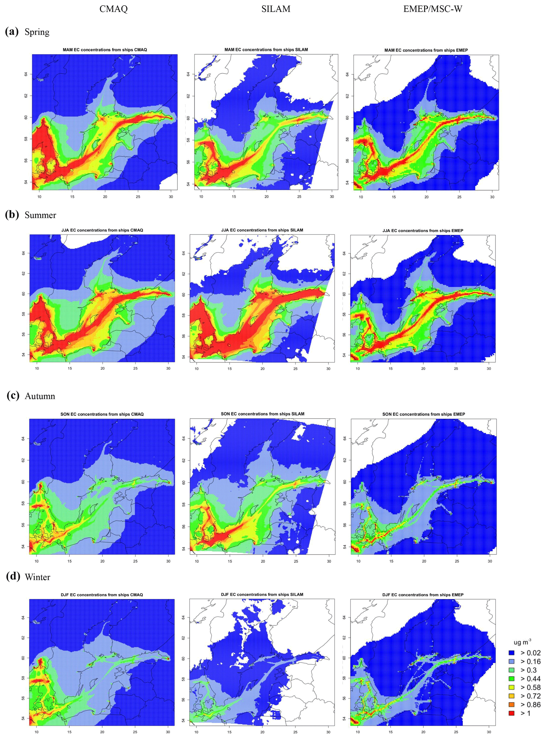
Figure 11 Spatial distribution of the seasonal mean EC ship contribution (µg m⁻³) from CMAQ (left column), SILAM (middle column) and EMEP (right column) in the Baltic Sea region for (a) spring, (b) summer, (c) autumn, and (d) winter. Empty areas correspond to concentrations between zero and the lowest value in the legend.

In stable conditions, the boundary layer (BL) height over the Baltic Sea is often at or below 500 m (Svensson et al., 2016; Gryning and Batchvarova, 2002). Climatological simulations over the Baltic Sea show that there is a strong seasonality in the atmospheric stability over the sea with more than 50 % stable conditions in spring, whereas during the other seasons unstable conditions dominate together with occasionally neutral conditions (Svensson et al., 2016). The lower surface concentrations of ship-related EC in SILAM and EMEP/MSC-W during spring compared to CMAQ might be attributed to different atmospheric stability in the simulations, i.e. more frequent occurrence of neutral conditions, which dilutes the concentration of the emitted pollutant. The fact that ship-related EC in EMEP/MSC-W is more confined to the shipping routes and shows a limited spatial spreading compared to the other models might also indicate less efficient horizontal diffusion. In winter, SILAM and EMEP/MSC-W ship-related EC is very low and the impacted area has a smaller extent than in the other months (white areas in Fig. 11), indicating faster removal of EC particles than in the CMAQ simulation. Different treatment of the hygroscopicity and ageing processes of EC particles, affecting their wet scavenging, could have contributed to the differences among the models.

4 Summary and conclusions

The effect of ship emissions on the regional air quality in the Baltic Sea region was investigated with three regional CTM systems (CMAQ, EMEP/MSC-W and SILAM) that simulate the transport, chemical transformation and fate of atmospheric pollutants. The models were applied with their typical set-up for air quality studies in European regions. The same ship emission dataset from the STEAM model based on ship movements from AIS records, detailed ship characteristics and up-to-date load-dependent emission factors were used in all CTMs. The models were set up with a finer grid resolution (4 to 11 km grid length) than was the case for previous air quality studies in the Baltic Sea region, potentially enabling better treatment of the dispersion and photochemistry in exhaust plumes from shipping along the major ship lanes of the Baltic Sea.

The comparison of total concentrations of regulatory air pollutants among the models is the primary focus of this study. Results from the three CTMs were compared to observations from rural and urban background stations of the AirBase monitoring network in the coastal areas of the Baltic Sea region. The finer resolution of CMAQ and SILAM (4 km) compared to EMEP/MSC-W (11 km) did not lead to a significant improvement in the urban bias and urban temporal correlation for daily mean NO₂ concentrations. The benefit from using high-resolution grids depends on the availability of accurate urban emission data with high spatial resolution (Schaap et al., 2015) and realistic temporal profiles (Kukkonen et al., 2012). While the STEAM inventory provides this data for shipping, the compilation of urban emission inventories is more challenging because they are based on specific information for each sector, such as housing units for domestic heating or number of vehicles (Guevara et al., 2016). Observed PM_2.5 in summer is underestimated strongly by CMAQ at all stations and to some extent by EMEP/MSC-W. Observed PM_2.5 in winter is underestimated by SILAM. In autumn all models are in better agreement with observed PM_2.5. The low summer PM_2.5 in CMAQ has been attributed to the underestimation of secondary organic aerosols and to the missing emissions of wind-blown soil dust particles (Karl et al., 2019). Particulate matter emissions from wind-blown dust and forest fires were included in EMEP/MSC-W and SILAM. Ship-related concentrations of NO₂ were evaluated at coastal monitoring stations by testing if the agreement between predicted and observed total concentrations improves significantly when ship emissions are included in the simulation. Including ship emissions improved the agreement between modelled and measured NO₂ daily mean concentrations at about 50 % of the stations. The change of modelled O₃ due to shipping was below 6 % on summer average at the shoreline stations and mainly reflects additional ozone production due to ship emissions. Ship-influenced stations identified by the models are mainly located close to the shoreline or close to a port, with a maximum distance of 20 km from the sea. However, modelled peaks of high daily mean NO₂ at coastal rural sites during summer that are not present in the measurements indicate that the models often did not properly resolve the ship plumes due to the subgrid variability of the plume dispersion of individual ships.

The spatial average of annual mean O₃ concentrations in the EMEP/MSC-W simulation is ca. 20 % higher compared to the other two simulations. EMEP/MSC-W overestimates the measurements of daily mean O₃ concentrations at rural stations by 17 % on average. The higher ozone concentrations in the EMEP model are mainly the consequence of using a different set of boundary conditions for the European model domain. The concentration gradients of NO₂ and SO₂ between urban and rural areas and between shipping lanes and the surrounding sea are larger in EMEP/MSC-W than in the other models. Factors contributing to the different gradients are differences in the representation of horizontal transport, differences in the meteorological driving data and differences in the atmospheric lifetime of NO₂ and SO₂ in the models.

There are significant differences in the calculated ship contributions to the levels of air pollutants among the three models. In the proximity of the main shipping routes, ozone is depleted as a result of the titration effect by NO emissions from shipping. Ozone depletion in EMEP/MSC-W is weaker than in the other two models, due to a combination of the larger grid cell volume causing higher initial dilution of ship emissions and of the use of monthly averages for ship emissions, averaging out hourly emission peaks.

The ship-related PM_2.5 affects the coastal areas in the Baltic Sea region, as its influence extends further inland than is the case for ship-related NO₂ and SO₂. The average contribution of ships to levels of PM_2.5 is calculated by the three CTMs ranges between 4.15 % and 6.5 % in the entire Baltic Sea region and between 3.15 % and 5.7 % in the coastal land areas. Differences in ship-related PM_2.5 among the models are mainly attributed to differences in the schemes for inorganic aerosol formation. Since shipping emissions of elemental carbon are identical in the three CTMs on a monthly basis, differences for ship-related EC can be explained by differences in the meteorological conditions, the treatment of atmospheric transport and the wet-scavenging parameterizations in the models.

Results obtained from the use of three CTMs give a more robust estimate of the ship contribution to atmospheric pollutant concentrations than a single model. By using several models the sensitivity of the ship contribution to uncertainties in boundary conditions, meteorological data as well as aerosol formation and deposition schemes is taken into account. This is an important step towards a more reliable evaluation of policy options regarding emission regulations for ship traffic and the introduction of a nitrogen emissions control area (NECA) in the Baltic Sea and the North Sea in 2021.

Appendix A: Statistical indicators

The performance of each model is quantified in terms of mean values (μ_Mod and μ_Obs), normalized mean bias (NMB), Spearman's correlation coefficient (R), root mean square error (RMSE) and FAC2.

The normalized mean bias is given by the following:

$$\begin{array}{}\text{(A1)}& {\displaystyle }{\displaystyle }\text{NMB}={\displaystyle \frac{\stackrel{\mathrm{‾}}{M}-\stackrel{\mathrm{‾}}{O}}{\stackrel{\mathrm{‾}}{O}}},\end{array}$$

where M and O stand for model and observation results, respectively. The overbars indicate the time average over N time intervals (number of observations). The time average is done for 1 year; hence $\stackrel{\mathrm{‾}}{M}$ corresponds to μ_Mod and $\stackrel{\mathrm{‾}}{O}$ corresponds to μ_Obs.

The Spearman's correlation coefficient is defined as the Pearson's correlation coefficient between the ranked variables. For a sample of size N, the N raw scores M_i and O_i for each time step i are converted to ranks rg(M_i) and rg(O_i). The Spearman's correlation coefficient is then computed from (Myers and Sirois, 2006)

$$\begin{array}{}\text{(A2)}& {\displaystyle }{\displaystyle }\mathrm{R}={\displaystyle \frac{\mathrm{cov}\left(\mathrm{rg}\right(M),\mathrm{rg}(O\left)\right)}{{\text{SDR}}_M\cdot {\text{SDR}}_O}},\end{array}$$

where cov(rg(M),rg(O)) is the covariance of the rank variables. SDR_M and SDR_O are the standard deviations of the ranks of the model and observation data. The Spearman correlation between two variables is equal to the Pearson correlation between the rank values of those two variables; while Pearson's correlation assesses linear relationships, Spearman's correlation assesses monotonic relationships (whether linear or not). If there are no repeated data values, a perfect Spearman correlation of +1 or −1 occurs when each of the variables is a perfect monotone function of the other.

The root mean squared error combines the magnitudes of the errors in predictions for various times into a single measure and is defined as follows:

$$\begin{array}{}\text{(A3)}& {\displaystyle }{\displaystyle }\text{RMSE}=\sqrt{{\displaystyle \frac{\mathrm{1}}{N}}\sum _{i=\mathrm{1}}^N{\left(M_i-O_i\right)}^{\mathrm{2}}}.\end{array}$$

RMSE is a measure of accuracy and allows prediction errors of different models to be compared for a particular dataset.

FAC2 is the fraction of model values within a factor of 2 of the observations (Hanna and Chang, 2012):

$$\begin{array}{}\text{(A4)}& {\displaystyle }{\displaystyle }\text{FAC2}::\text{fraction, where }\mathrm{0.5}\le {\displaystyle \frac{M_i}{O_i}}\le \mathrm{2}.\end{array}$$

Appendix B: Time series plots

The appendix contains the time series plots of NO₂ concentrations at selected ship-influenced monitoring stations for the meteorological year 2012. Time series plots of O₃ concentrations at the corresponding sites are shown in Fig. S1.

Figure B1 Ship influence on daily mean NO₂ concentration (µg m⁻³): (a) EE0011A, (b) FI00349, (c) SE0066A, (d) DESH023, (e) FI00351, (f) EE0009R, (g) PL0053A, (h) PL0171A, (i) DEMV021, (j) DESH033, (k) DK0053A, and (l) SE0022A. Model data from CMAQ (dark red line), SILAM (blue line), EMEP/MSC-W (green line), the respective noship run (dashed red line) and observations (black line with open circles).