the Creative Commons Attribution 4.0 License.
the Creative Commons Attribution 4.0 License.
 | 20 May 2019
The unintended consequence of SO2 and NO2 regulations over China: increase of ammonia levels and impact on PM2.5 concentrations
Mathieu Lachatre
Audrey Fortems-Cheiney
Gilles Foret
Guillaume Siour
Gaëlle Dufour
Lieven Clarisse
Cathy Clerbaux
Pierre-François Coheur
Martin Van Damme
Matthias Beekmann
Air pollution reaching hazardous levels in many Chinese cities has been a major concern in China over the past decades. New policies have been applied to regulate anthropogenic pollutant emissions, leading to changes in atmospheric composition and in particulate matter (PM) production. Increasing levels of atmospheric ammonia columns have been observed by satellite during recent years. In particular, observations from the Infrared Atmospheric Sounding Interferometer (IASI) reveal an increase of these columns by 15 % and 65 % from 2011 to 2013 and 2015, respectively, over eastern China. In this paper we performed model simulations for 2011, 2013 and 2015 in order to understand the origin of this increase and to quantify the link between ammonia and the inorganic components of particles: . Interannual change of meteorology can be excluded as a reason: year 2015 meteorology leads to enhanced sulfate production over eastern China, which increases the ammonium and decreases the ammonia content, which is contrary to satellite observations. Reductions in SO2 and NOx emissions from 2011 to 2015 of 37.5 % and 21 % respectively, as constrained from satellite data, lead to decreased inorganic matter (by 14 % for ). This in turn leads to increased gaseous NH3(g) tropospheric columns by as much as 24 % and 49 % (sampled corresponding to IASI data availability) from 2011 to 2013 and 2015 respectively and thus can explain most of the observed increase.
- Article
(11841 KB) - Full-text XML
-
Supplement
(19308 KB) - BibTeX
- EndNote


Particulate matter (PM) pollution poses serious health concerns all over the world and particularly over China (Cohen et al., 2017; Landrigan et al., 2017). Among PM precursors, several studies (Seinfeld and Pandis, 2006; Schaap et al., 2004; Lelieveld et al., 2015; Bauer et al., 2016; Pozzer et al., 2017) pointed out the importance of ammonia (NH3(g)), whose main source is agriculture and which acts as a limiting species in the formation of fine particulate matter (PM2.5, particulate matter with an aerodynamic diameter less than 2.5 µm; Banzhaf et al., 2013). Balance between SO2, NOx and NH3 emissions will define cation- or anion-limited regimes of inorganic particulate matter formation, and this is key for PM control policies (Paulot et al., 2016; Fu et al., 2017). Yet, an increase in the ammonia atmospheric content over China has been observed by the satellite instrument AIRS, with a trend of +2.27 % yr−1 from 2002 to 2016 (Warner et al., 2017). Infrared Atmospheric Sounding Interferometer instrument (IASI) satellite observations (Van Damme et al., 2017) also show an increased density of the NH3(g) column over China between 2011 and 2015, with a sharper trend between 2013 and 2015. Several factors could explain this enhancement, including an increase of NH3(g) emissions in China, whereby agricultural activities represent 80 %–90 % of total ammonia emissions in China (Kang et al., 2016). However, ammonia emissions appear to have reached a maximum in 2005 and have been almost constant since (Kang et al., 2016). Another study (Zhang et al., 2018) estimates a 7 % increase of NH3 emissions between 2011 and 2015, much lower than the observed trends. Other sources, such as biomass burning and associated ammonia emissions, do not show particular trends (Wu et al., 2018). Consequently, the increase of atmospheric NH3(g) concentrations over China does not seem to be explained by changes in ammonia emissions. The rise of ammonia concentrations over China could be explained by increased NH3(g) evaporation from inorganic PM due to a rise in temperature, as shown by Riddick et al. (2016). Meteorological variations would change both the NH3(g) volatilization and the equilibrium between ammonia, ammonium nitrate (NH4NO3) and nitric acid (HNO3). Finally, a decrease in sulfate and total nitrate availability caused by SOx (SO2 + ) and NOx (NO + NO2,) emission reductions (Liu et al., 2017; de Foy et al., 2016) could leave more ammonia in the gas phase, since less ammonium is required to neutralize particle-phase acids, following a mechanism already observed by Schiferl et al. (2016) over the United States. Such a decrease in SO2 emissions has also occurred over China since 2011 (Koukouli et al., 2018). Its impact on atmospheric ammonia concentrations has not been quantified yet. Wang et al. (2013) examined the change of Chinese sulfate–nitrate–ammonium aerosols due to anthropogenic emission changes of SO2 and NOx from 2000 to 2015. However, they assumed an increase of NOx emissions from 2006 to 2015 and not the large decrease observed since 2013.
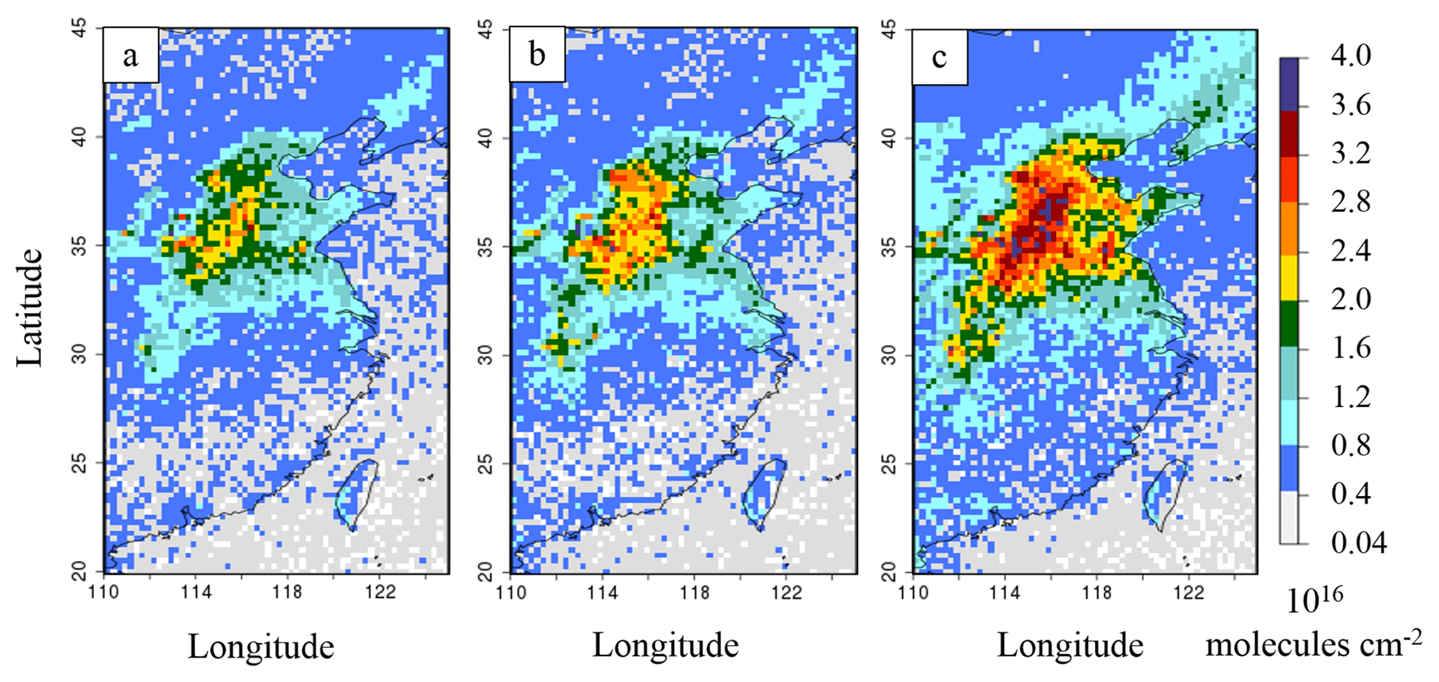
Figure 1IASI instrument NH3(g) total columns over eastern China (110–125∘ E, 20–45∘ N), in 1016 molecules cm−2 for (a) 2011, (b) 2013 and (c) 2015. In this figure, the available observations have been averaged on a 0.25∘ × 0.25∘ grid.
A recent study by Liu et al. (2018) suggests that ammonia increase mainly comes from SO2 emission policies. They found that the changes in NOx emissions decreased the NH3 column concentrations in their study period. Conversely, Fu et al. (2017) have shown that SO2 and NO2 emissions control was an important factor affecting the significant enhancement of NH3 column concentrations over China during the period 2011–2014. In addition, our study also presents a comparison to NH3 IASI satellite observations. Our goal here is to understand the factors controlling atmospheric ammonia concentrations over China in recent years. In order to identify the drivers of NH3(g) variability over China, we conducted different sensitivity studies with a regional chemistry-transport model, isolating the impacts of (i) meteorological conditions and (ii) decrease of anthropogenic SO2 and NOx emissions. Section 2 presents the regional chemistry-transport model (CTM) CHIMERE used in this study and the different settings of the performed sensitivity tests. It also presents IASI NH3 column and surface PM observations. Section 3 gives the results of the sensitivity tests and shows the impacts of meteorological conditions and emission changes on ammonia and ammonium concentrations. The simulations are also evaluated by comparison of the modelled PM2.5 concentrations with surface measurements. Finally, the modelled NH3(g) column interannual variability is compared to that retrieved from satellite (IASI) data.
2.1 IASI satellite observations
NH3(g) column observations from space are provided by the Infrared Atmospheric Sounding Interferometer instrument (IASI), operating between 3.7 and 15.5 µm, on board the Metop-A European satellite (Clarisse et al., 2009; Van Damme et al., 2018). The algorithm used to retrieve NH3 columns from the radiance spectra is described in Whitburn et al. (2016) and Van Damme et al. (2017).
For this study we used the dataset ANNI-NH3-v2.2R-I, relying on ERA-Interim ECMWF (European Centre for Medium-Range Weather Forecasts) meteorological input data rather than the operationally provided EUMETSAT IASI Level 2 (L2) data used for the standard near-real-time version. An analysis of ANNI-NH3-v2.1 time series revealed sharp discontinuities coinciding with IASI L2 version changes (Van Damme et al., 2017). With the ECMWF ERA-Interim reanalysis, the time series is now coherent in time (except for the cloud coverage flag) and can therefore be used to study interannual NH3(g) variability over eastern China between 2011 and 2015 (Fig. 1). We used the daily satellite information from morning orbits (at ∼09:30 LT) to have daily information on IASI data availability. The IASI total columns are first averaged into daily “super-observations” (average of all individual IASI data within the 0.25∘ × 0.25∘ resolution of CHIMERE). The annual gridded means of Fig. 1 are calculated from these gridded daily super-observations. In this study, and as suggested in Van Damme et al. (2017), we do not apply a selection to the IASI observations. In 2011, a mean value of 4.7×10¹⁵ molecules cm−2 is observed for eastern China, increasing to 5.36×10¹⁵ molecules cm−2 in 2013 (+15 %) and 7.76×10¹⁵ molecules cm−2 in 2015 (+65 %).
2.2 The chemistry-transport CHIMERE model and updated NOx and SO2 emissions
CHIMERE (2014b version) is a three-dimensional chemistry-transport regional model (Menut et al., 2013; Mailler et al., 2017; http://www.lmd.polytechnique.fr/chimere/, last access: 15 September 2018) run here over a 0.25∘ × 0.25∘ regular grid, on a domain completely covering China's territory (–145∘ E, –55∘ N). The domain includes 290 (longitude) grid cells × 150 (latitude) grid cells and 17 vertical layers, with altitude going from the ground to 200 hPa (about 12 km), with eight layers within the first 2 km. Meteorological fields are provided by ECMWF meteorological forecasts (Owens and Hewson, 2018; Jingjing et al., 2015; Chen et al., 2010). To prescribe atmospheric boundaries and initial composition, climatological values are used from the LMDZ-INCA global model (Szopa et al., 2008). Biogenic emissions are calculated taking into account meteorological parameters with the MEGAN-v2 model (Guenther et al., 2006). We use the EDGAR-HTAP-v2.2 inventory delivered for the year 2010 (Janssens-Maenhout et al., 2015), to prescribe the anthropogenic emissions for the simulation. Chinese emissions in EDGAR-HTAP-v2.2 are derived from the Multi-resolution Emission Inventory for China (MEIC) developed by Tsinghua University, the NH3(g) emission inventory from Peking University (Huang et al., 2012) and the Regional Emission inventory in Asia (REAS) (Kurokawa et al., 2013) to fill the remaining gaps. The respective total annual emissions of SO2, NO and NH3(g) for 2010 are 42.4, 25.2 and 20.3 Mt (Table 1), and the spatial distributions of these emissions are represented in Fig. 2.
Table 1Annual budgets of the EDGAR-HTAP-v2.2 inventory and of emissions corrected from the OMI instrument (this work), for SO2, NO and NO2, over Asia and over eastern China (in Mt). The Asian domain corresponds to our full domain (–145∘ E, –55∘ N), and the eastern China domain corresponds to a smaller domain (110–125∘ E, 20–45∘ N), displayed by a black rectangle in Fig. 2.
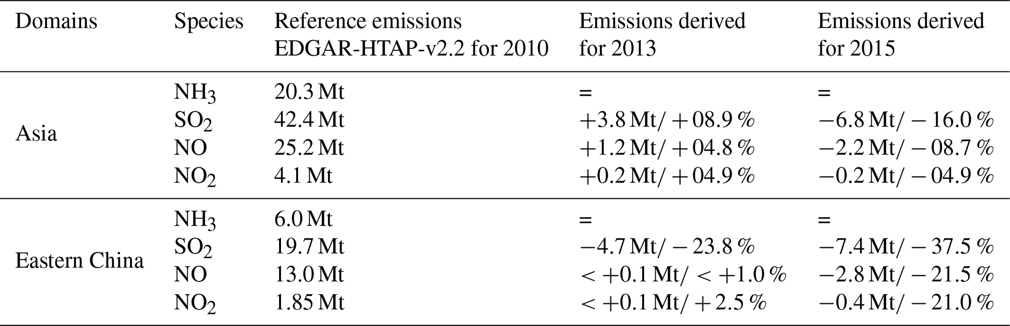
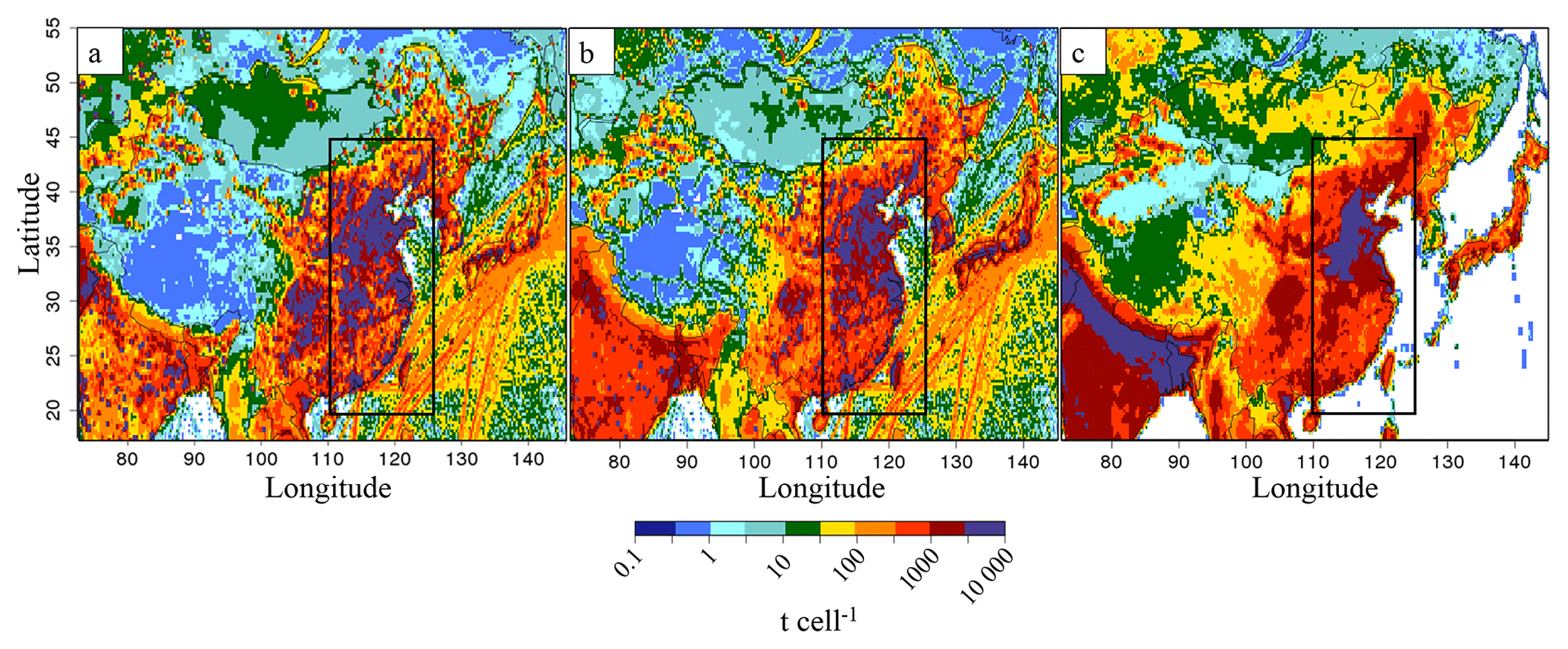
Figure 2EDGAR-HTAP-v2.2 emissions for the year 2010 for (a) SO2, (b) NO and (c) NH3. Units are tons per cell (t cell−1) (cell size of 0.25∘ × 0.25∘). The black rectangle shows the eastern China domain.
We used the most recent HTAP emission inventory built for the year 2010 to simulate emissions of the year 2011, assuming that both years have similar emissions. Initially, a comparison of the OMI and CHIMERE NO2 columns for 2011 shows a Pearson correlation coefficient of 0.78 for daily values and an annual mean bias of −7 %. To understand the impact of the NOx and SO2 emission reductions observed over China in 2013 and 2015, the model emissions need to be updated. The observed variability of satellite columns has been used to update emissions, as in Palmer et al. (2006). Here NO, NO2 and SO2 emissions have been updated following the variability observed by OMI between 2011, 2013 and 2015. We assume that NO2 variations are controlled by NOx emissions changes. The yearly gridded relative variabilities seen by the OMI instrument between 2011 and 2013 and between 2011 and 2015 are applied to daily prior anthropogenic SO2, NO and NO2 emissions. H2SO4 emissions represent only a small fraction of SOx (1 %) and, consequently, are not updated here. Equation (1) has been applied to each pixel of our regional grid for 2015 and 2013, where i can be SO2, NO2 or NO and j the pixel number:
Emis(2010) represents the reference HTAP emission inventory, and Col(2011) and Col(year) the respective OMI satellite observation values for 2011 and 2015 (or 2013). Corrections for the emission inventory are shown in Fig. 3. Values of derived emissions have been limited to 500 % of initial values, to avoid outlier values located in North Korea. It should be noted that our update based on annual averages does not modify the seasonal cycle for NOx and SO2 (with a maximum in winter; see Fig. S1 in the Supplement). In the model, spatial distributions for NOx and SO2 emissions appear to have a similar structure (see Fig. 2). Ammonia emissions show a significant seasonal cycle with emissions higher during summer than during the other seasons. On a molar basis, NH3(g) emissions are low compared to SO2 and NOx emissions, except in summer when NH3(g) emissions are in excess compared to SO2 alone (Fig. S1 in the Supplement).

Figure 3Annual differences between the EDGAR-HTAP-v2.2 inventories for the year 2010 and the emissions corrected from OMI for the year 2015, for (a) SO2, (b) NO and (c) NO2. Units are tons per cell (t cell−1) (cell size of 0.25∘ × 0.25∘).
When applying Eq. (1), the temporal evolution of OMI NO2 columns leads to a decrease in NOx emissions (Figs. S3 and S4 in the Supplement), particularly after 2013 (+1 % in 2013 and −21 % in 2015 as compared to 2011). Liu et al. (2017) derived similar NOx emission changes with the exponentially modified Gaussian method of Beirle et al. (2011) (e.g. decrease of 21 % of NOx emissions within Chinese cities between 2011 and 2015). We have also compared our updated inventories for NOx and SO2 with the DECSO v5 inventories calculated with an inverse modelling method based on an extended Kalman filter (Mijling and Zhang, 2013; Ding et al., 2017; http://www.globemission.eu/, last access: 4 July 2018). For DECSO, the a priori NOx anthropogenic emissions are taken from the EDGAR-v4.2 inventory, whereas our prior emissions come from EDGAR-HTAP-v2.2. EDGAR-v4.2 does not take into account shipping emissions, as shown in Fig. S2 in the Supplement. Our annual evolution rates are consistent with DECSO trend estimates (+1 % in 2013 and −14 % in 2015, compared to DECSO in 2011). A recent study from Zheng et al. (2018) evaluated NOx emissions and found a change of −17.4 % from 2011 to 2015, similar to our −24 % change. The OMI SO2 trends imply (following Eq. 1) a continuous decrease of SO2 emissions from 2011 to 2015 (−24 % in 2013 and −37 % in 2015 compared to 2011; see Table 1 and Fig. 2a). This decreasing trend is consistent with trend estimates of the SO2 in DECSO, −11 % in 2013 and −25 % in 2014 compared to 2011. Nevertheless, our total SO2 emissions in 2013 seem to be underestimated compared to the DECSO annual estimates (−15 % in 2011, −25 % in 2013). It should be noted here that our method to update emissions has some limitations. All the variability of satellite tropospheric columns is attributed to emissions, without taking into account variability associated to meteorology, transport, chemistry or instrumental degradation. However, the comparison with independent emission estimations shows good consistency. Zheng et al. (2018) found SO2 emissions change of −41.9 % between 2011 and 2015, again similar to our −37.5 % evolution. Hence, we consider our estimated emission inventories realistic enough to conduct sensitivity tests.
The emission update helped correctly reproduce the column changes for SO2 −44 % (CHIMERE) and −53 % (OMI) between 2011 and 2015 and for NO2 −31 % (CHIMERE) and −23 % (OMI) between 2013 and 2015.
2.3 ISORROPIA
The composition and phase state of inorganic aerosol in thermodynamic equilibrium with gas-phase precursors are calculated using the ISORROPIA V2006 module (Nenes et al., 1998). The CHIMERE CTM calculates the thermodynamical equilibrium of the system: sulfate–nitrate–ammonium–water for a given temperature (in a range [260–312 K]; increment: ΔK =2.5 K) and relative humidity (RH, in a range [0.3–0.99]; increment: ΔRH =0.05). Considering temperature, relative humidity, TN (TN = + HNO3; total nitrates), TA (TA = + NH3(g); total ammonia) and TS (TS = + H2SO4; total sulfates), the gas to particle partitioning of and is calculated using tabulated values. Depending on the equilibrium calculation, both the absorption and desorption of ammonia are represented in the model. Within CHIMERE, a kinetic approach is also added to simulate transport barriers for the gas to the particle phase and vice versa. Over Europe, a recent study, conducted with CHIMERE and the ISORROPIA V2006 module, showed that higher temperature and lower RH will promote NH3(g) at the expense of (Petetin et al., 2016).
2.4 Set-up of the performed sensitivity tests
Six experiments were performed to discriminate factors that control the ammonia atmospheric budget over China over recent years. Configurations corresponding to the six experiments are described in Table 2. The 2011 reference simulation serves as a baseline for comparison with the other simulations (under different meteorological and emissions scenarios). The simulations labelled “A” are used to quantify the influence of meteorological parameters, the simulation labelled “B” to quantify the influence of SO2 emissions variations and simulations labelled “C” to quantify the influence of both SO2 and NOx emissions variations. The 2013A and 2015A simulations were performed keeping emissions at 2010 levels, but the meteorology was updated to isolate effects of meteorological variability on simulated ammonia levels. Among scenarios performed in our study, the 2015B simulation uses the same meteorology as 2015A but with 2015 SO2 emission giving information on the role of Chinese SO2 emission reduction in the NH3(g) atmospheric content. Finally, the 2015C simulation uses the same meteorology as 2015A but using both SO2 and NOx emissions corrected with 2015 OMI observations (see Table 2). As the updated 2013 NOx emissions are similar to the initial EDGAR-HTAP-v2.2 emissions used for the 2011 reference simulation, we expect similar results for the 2013B and 2013C simulations. Consequently, the 2013B simulation was not conducted. Hence, 2013C and 2015C are the key simulations of our study showing the combined effect of SO2 and NOx emission reductions and of meteorology on atmospheric ammonia.
Table 2Description of the different experiments performed with the regional chemistry-transport model CHIMERE.

3.1 Impact of meteorological conditions on the ammonia/ammonium–sulfate–nitrate system
Three scenario simulations using the same emissions but different meteorological conditions (2011A, 2013A and 2015A) were performed to understand the role of meteorology in ammonia atmospheric concentrations. As our study uses satellite observations giving tropospheric trace gas columns for different purposes, the model results will be generally presented as vertical columns (reaching from the ground to 12 km height). However, most of the column content can generally be found within the first 2.5 km, close to the ground (more than 90 % of NH3(g) is located within the first 2.5 km in CHIMERE). Hence, to study the meteorological influence on ammonia, we restrict the comparison to 0 to 2.5 km (which corresponds to about 720 hPa) partial columns, as we want to average meteorological parameters for a height that should be representative of conditions where pollutants are located. Figure 4 shows NH3(g) columns in 2011 (Fig. 4a) and simulated variations depending on meteorological conditions for 2013 (Fig. 4b) and 2015 (Fig. 4c). It can be observed that the eastern China area includes regions with the highest NH3(g) values (except the Indo-Gangetic Plain). Over the eastern China area, meteorological conditions affect NH3(g) columns: an increase of 4 % is simulated in 2013, whereas a decrease of 7 % is simulated in 2015. In addition, it can be observed that over the southern China area (see black rectangle in Fig. 4b–c) ammonia decreases for 2013 and 2015.
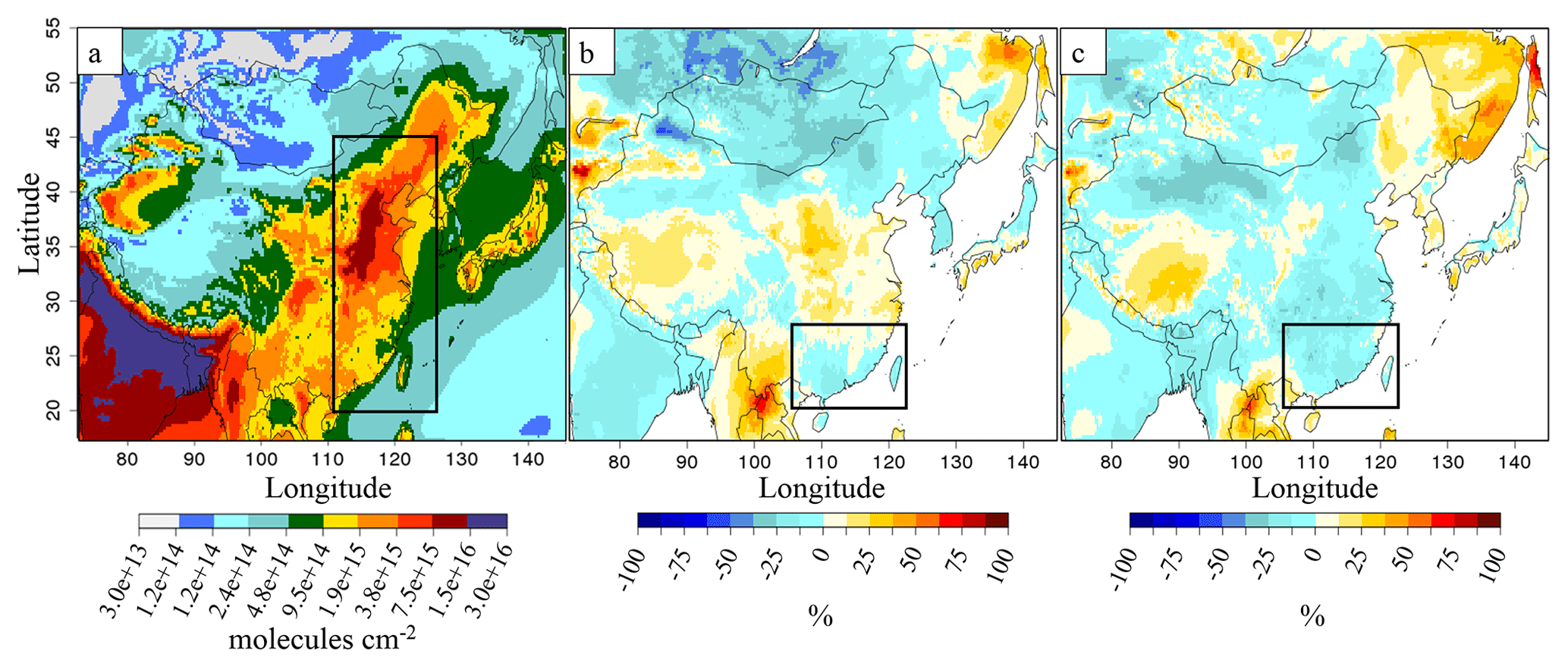
Figure 4(a) Ammonia columns (molecules cm−2) for the 2011A simulation; (b) relative differences (%) of ammonia columns between 2013A and 2011A; (c) relative differences between 2015A and 2011A. Note that as values over the sea mostly represent only small variations, we do not show them here and in the following figures.
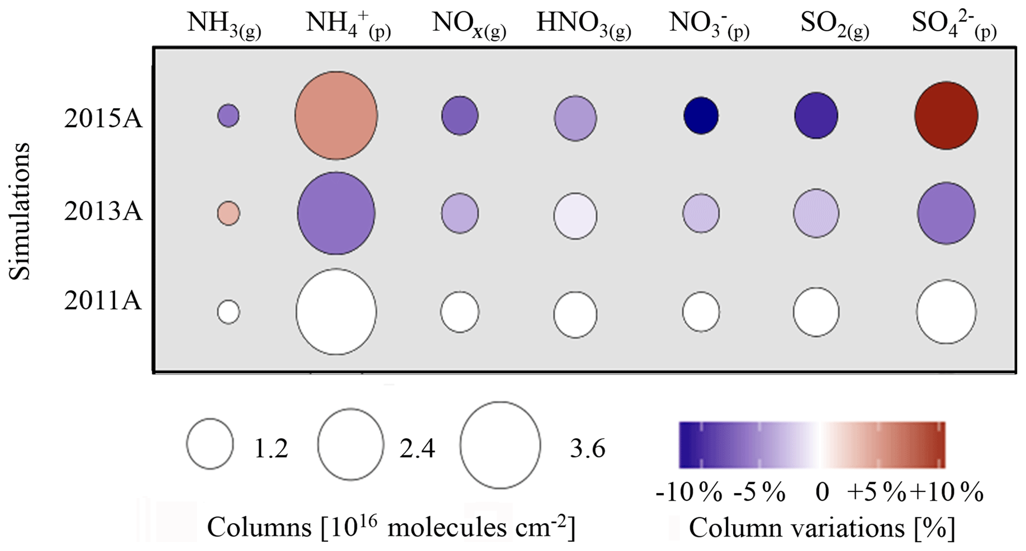
Figure 5Gaseous and particulate inorganic species variation for the eastern China region. Disk surfaces are proportional to column amount (molecules cm−2) and colours indicate relative evolution rates compared to 2011A (%).
Figure 5 shows that ammonia changes caused by meteorological variations are opposite to sulfate and ammonium changes in both cases, for 2013 and 2015. Meteorological conditions in 2015 (Fig. S5 in the Supplement) promoted the formation of ammonium and sulfates (+6 % and +12 % respectively) in 2015A compared to 2011A and a decrease of nitrates (−13 %; Fig. 5). For 2013, changes of NH3(g) are opposite to ammonium (−7 %) and sulfates (−7 %), with a slight increase of NH3(g) (+4 %). It appears that changes in the ratio are correlated with changes. This can be explained from well-known neutralization reactions in the gas (Reaction R1) or aqueous phase (Reactions R2 and R3):
SO2 oxidation to can happen in the gas phase, from process Reaction (R5), in which OH is the oxidant, produced from Reaction (R4), that is linked to humidity:
Sulfate production can also occur in the aqueous phase, by SO2(aq) oxidation with O3 or H2O2, yielding sulfuric acid which can then be neutralized to form ammonium sulfate (Hoyle et al., 2016). The extent of this reaction chain depends on cloud liquid water content. It is initiated by a solution of SO2(g) in the water phase (SO2•H2O(aq)):
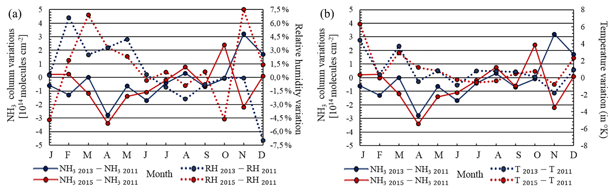
Figure 6(a) Monthly variation of NH3(g) partial columns and relative humidity in 2013 and 2015 compared to 2011. (b) Monthly variation of NH3(g) partial columns and temperature in 2013 and 2015 compared to 2011.
While the aqueous-phase pathway is globally dominant, the gas-phase pathway can also be important under dry conditions (e.g. Seinfeld and Pandis, 2006). In our study, we did not investigate the relative importance of both pathways because this would have required inclusion of specific tagging. Nevertheless, for both pathways, RH increase favours production, either through increased production of OH radicals in the gaseous phase (for a given temperature, so that specific humidity also increases) or through a larger cloud liquid water content (Hedegaard et al., 2008). In 2013, annual mean temperature and annual mean RH increased by +0.7 K and decreased by −0.9 % respectively compared to 2011; cloud liquid water relative variation also shows a decrease of −7 %. In 2015, temperature and annual mean RH increased by 1 K and increased by +1.3 % respectively compared to 2011, and cloud liquid water relative variation increased by +20 %. Accordingly, the total sulfate–nitrate–ammonium (called pSNA hereafter) production is increased by +7 % in 2015A compared to 2011A, which explains the decrease in the NH3(g) columns of −7 %. Conversely, meteorological conditions in 2013 (decrease of RH and liquid water) depressed the formation of pSNA (Fig. 5). Consequently, its production was lower by about 6 % in 2013A compared to 2011A, and NH3(g) columns were larger by +4 %. These relationships between meteorological parameters and NH3(g) columns can also be documented by correlation statistics (Fig. 6). An inverse correlation between monthly RH and NH3(g) column variations over the eastern China domain is shown in Fig. 6a, with Pearson correlation coefficients of −0.47 and −0.56 in 2013 and 2015, respectively. An even more pronounced negative correlation is also observed on a daily basis, with correlation coefficients for 2013 and 2015 of −0.71 and −0.61 respectively. When RH increases, the production of from NH3(g) also increases. The largest difference between 2013A and 2015A is observed in November and December 2013 and 2015, when RH variations and NH3(g) column variations are opposite (Fig. 6a). Figure 6b shows that temperature changes do not control the NH3(g) variation, as the Pearson correlation coefficients are −0.04 and 0.09 in 2013 and 2015 respectively. It should also be noted that decreases of ammonia and ammonium are observed over areas showing an increase in rainfall frequencies (see Fig. S6 in the Supplement) in 2015 and 2013 (in the south of China, Guangxi and Guangdong Province; see the black box in Fig. 4). Conversely, with rainfall frequencies lower than 90 d yr−1 (for rainfall above 1 mm d−1), and small changes in rainfall frequencies over the North China Plain for 2011 and 2013, changes in wet deposition do not seem to impact ammonia levels significantly. Indeed, low correlation is found between monthly rainfall frequency variations and monthly ammonia variations over eastern China (Pearson correlation coefficients of −0.12 and −0.18 for 2013 and 2015 respectively).
Finally it has been observed in this study that total NH3(g) + columns will vary depending on meteorological conditions. It should be noted that if NH3(g) is favoured, as for 2015, the total content will decrease as NH3(g) lifetime is shorter than lifetime due to faster deposition.
3.2 Impact of SO2 and NOx emission reduction on NH3 columns and inorganic aerosol
3.2.1 Impact of SO2 and NOx emission reduction on NH3 columns
Figure 7b represents the impact of the SO2 emission reduction on NH3(g) columns for the 2015B simulations. For the year 2013, the comparison is made from the 2013C simulation (see Table 1, and Fig. S7 in the Supplement), since NOx emissions between 2011 and 2013 are similar. The SO2 emission reduction (−24 % for 2013 and −37 % for 2015 as compared to 2011) strongly affects NH3(g) columns, which increase by +10 % over eastern China in the 2013C simulation compared to 2013A and by about +36 % in the 2015B simulation compared to 2015A. Thus, the effect of SO2 reduction on NH3(g) columns appears to be non-linear because NH3(g) interactions are not limited to SO2. It should be noted that the column change is mainly controlled by changes between the surface and the first few kilometres of altitude, as much of column content (>90 %) is located between the surface and 2.5 km of altitude; but as IASI and OMI satellite provide full column information, we present the entire CHIMERE column to be as consistent as possible with observations. In the two cases, the decrease of ammonia over western China and Mongolia (between 0 % and −15 %; Fig. 7b), where NH3(g) values are initially low (Fig. 7a), remains small. Figure 7c shows the additional impact of NOx emission reductions, of about −21 % between 2015 and 2011, on the NH3(g) amount over eastern China (with the 2015C simulation, compared to 2015B). The additional increase of ammonia columns in the 2015C simulation, is about 15 % compared to the 2015B simulation (SO2 emission decrease only) in the northern part of the eastern China subdomain. This statement on NOx emission evolution impacts is different from that in Liu et al. (2018), in which NOx emission reduction is considered not responsible for the NH3 increase between 2011 and 2015.

Figure 7(a) Ammonia columns (molecules cm−2) for the 2015A simulation, (b) relative differences of ammonia columns between the simulations from 2015B and 2015A, in %, and (c) additional relative differences of ammonia columns between the simulations from 2015C minus 2015B compared to 2015A, in %. The black rectangle is for the eastern China domain.
Figure 8b represents the impact of the SO2 emission reductions on columns with a decrease of about 14 % in the 2015B simulation compared to 2015A. The reduction of NOx emissions between 2015B and 2015C leads to an additional decrease of ammonium levels in the 2015C simulation, −4 % compared to 2015B for eastern China, where the decrease is most pronounced (Fig. 8c). In addition, ammonium columns have decreased by about 2 % over eastern China in the 2013C simulation compared to 2013A. The spatial anti-correlation observed between and NH3(g) is explained by less production of from the NH3(g) due to emission modifications. It is interesting to note that the NOx and SO2 emission reduction impacts on NH3(g) and columns can differ depending on the area (see Fig. S8 in the Supplement). In the 2015B simulation the ammonium production decreases most strongly in the Sichuan Province and Chongqing municipality (black rectangle, Fig. 8b), and there is a large-scale decrease around SO2 sources (Fig. 2a). In the 2015C simulation, we can observe a larger decrease in the northern China region (red rectangle, Fig. 8c), where ammonium nitrate is produced with freshly formed HNO3(g), following Reaction (R8):
These relationships between sources and impacted regions are explained by the time needed for and formation from SO2 and NOx precursors of several days and several hours to 1 d respectively. Thus, SO2 to H2SO4 oxidation is more a regional process (unless it happens in the aqueous phase), whereas nitrate formation proceeds closer to the sources. However, for conditions of weak atmospheric dispersion or high humidity, as in the Sichuan Province and Chongqing municipality (located in an orographic depression), sulfates can be formed closer to sources. In this area, sulfates contribute as much as 32 % to the PM column, compared to 23 % over eastern China, (Fig. S8 in the Supplement).
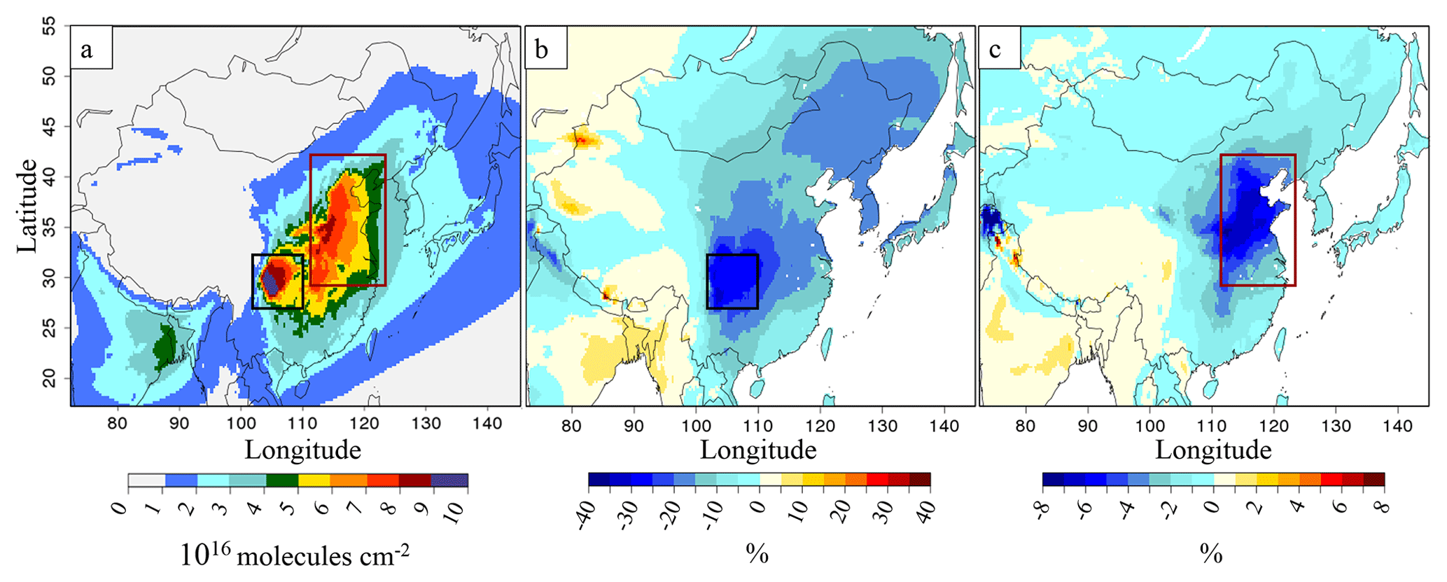
Figure 8(a) Ammonium columns (molecules cm−2) for the 2015A simulation, (b) relative differences of ammonium columns between the simulations from 2015B and 2015A, in %, and (c) additional relative differences of ammonium columns between the simulations from 2015C minus 2015B compared to 2015A, in %. The black rectangle is for the Sichuan Province and Chongqing municipality, and the red rectangle is for northern China.
3.2.2 Impact of SO2 and NOx emission reduction on pSNA production
The emission update leads to changes in the pSNA production, as already suggested by changes in the columns. As SO2 columns are strongly decreased (−40 % for 2015B; −41 % for 2015C), less ammonium (−14 % for 2015B; −18 % for 2015C) is formed in the particulate phase from the reaction with sulfuric acid (Reactions R1, R2, R3), and more NH3(g) remains in the gas phase (+36 % for 2015B; +51 % for 2015C; see Figs. 9 and S9 in the Supplement). These higher NH3(g) levels trigger a larger conversion (Reaction R8) of gaseous nitric acid into particulate (+33 %; Figs. 9 and S10). In the 2015C simulation, the increase of is less notable (+11 % because NOx emissions decrease), and ammonia columns show a bigger increase than in 2015B over eastern China. On the whole, the reduction of emissions in the 2015B and 2015C simulations leads to a reduction of the total pSNA PM production (e.g. −16.6 % and −18.5 %, respectively, compared to 2015A), mainly promoted by the reduction of SO2 emissions. Among PM components, a decrease of the sulfate molar fraction is observed (from 32 % to 29 %), and the fraction increases, from 12 % to 15 %, while the molar fraction stays stable around 56 % (21 % of pSNA PM mass). It can also be observed in these scenarios that for similar emissions and meteorology, TA decreases in 2015B and slightly more in 2015C (Fig. S9 in the Supplement). The reasons are that ammonia is favoured compared to 2015A and that deposition is a more efficient process for ammonia.
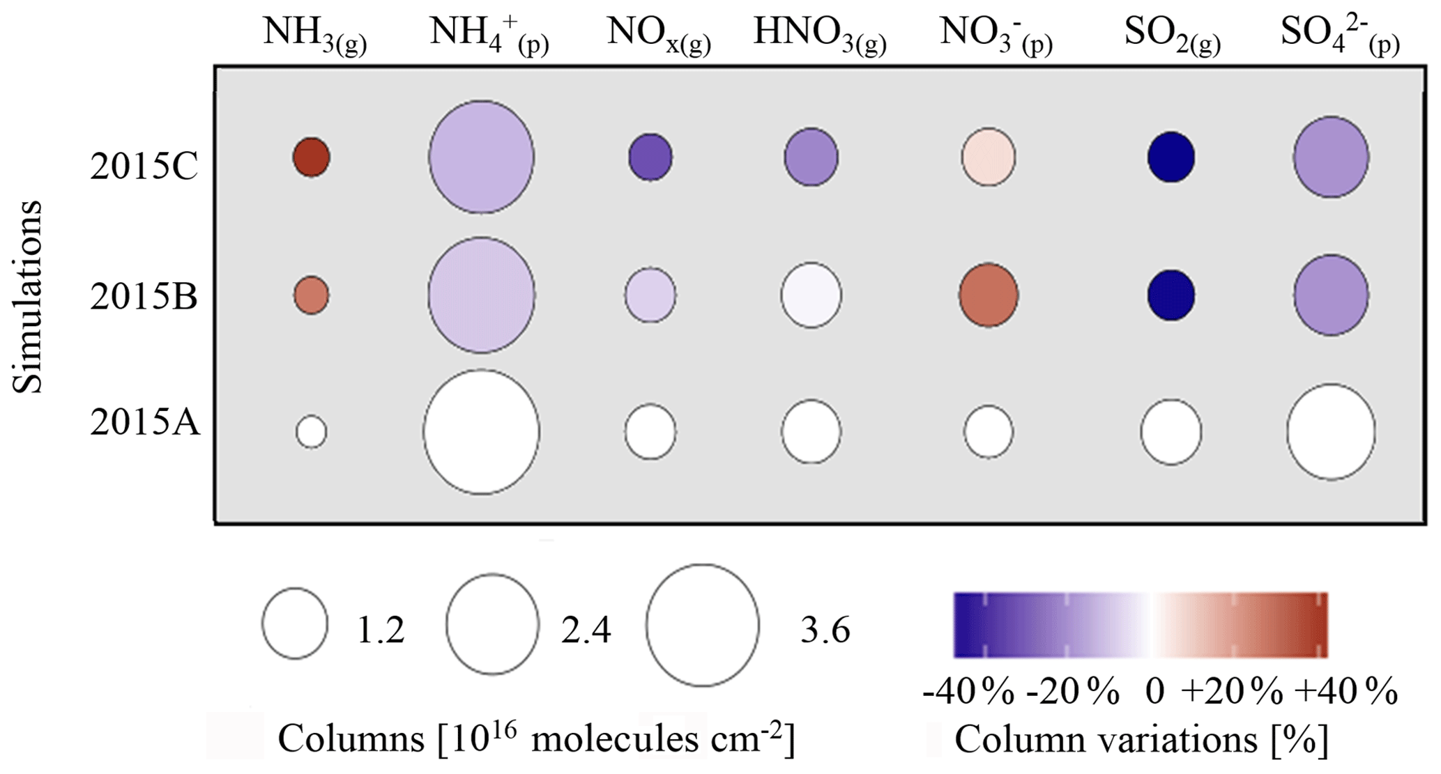
Figure 9Gaseous and particulate inorganic species variation for the eastern China region. Disk surfaces are proportional to column amount (molecules cm−2), and colours indicate relative evolution rates compared to 2015A (%).
3.2.3 NH3(g): a key role in the regulation of PM pollution as a limiting reactant
The regime of nitrate production, limited either by NH3(g) or HNO3(g), can be evaluated using the Gratio calculation (Ansari and Pandis, 1999; Pinder et al., 2008; Gratio two-dimensional distribution is displayed in Fig. S10 in the Supplement). A negative value of the Gratio indicates that TA low availability is strongly limiting nitrate production in competition to sulfate production, while a value in the range [0–1] indicates a TA-limited situation, and a value greater than 1 indicates that TA is in excess. In our study, as we want to know if we are facing a cation- or anion-limited regime, we chose to adapt the Gratio to a cation ∕ anion ratio (C∕Aratio), easier to interpret with no negative values, as follows:
where TA is the total ammonia reservoir, and TN is the total nitrate reservoir. When the C∕Aratio is in the range [0–1] molC mol, we are in a cation-limited regime, and when C∕Aratio is larger than 1 molC mol, we are in an anion-limited regime. The C∕Aratio has been calculated for columns, partial columns (up to 1 km) and for the surface, and results for various scenarios are displayed in Fig. 10. It should be noted that the ratio has an important month-to-month variability (normalized standard deviation of 10 %), as displayed in Fig. 10d for the East Asia region. Note that is the only cation considered here; the potential role of other cations is discussed below. Figure 10d presents the C∕Aratio for the simulations considering several altitudes, at the surface, the 0–1 km column and the CHIMERE total column. C∕Aratio is highly variable depending on the vertical layer considered, with a significantly lower C∕Aratio considering a total column than a reduced layer close to the surface, a statement also observable in Paulot et al. (2016). Close to sources (surface), more ammonium will be present, leading often in the 2015B and 2015C scenarios to an excess cation regime. If we consider vertical columns, as 0–1 km for example (which corresponds roughly to the atmospheric mixing layer), the ratio is below 1 (anion-limited regime) for most months. Considering the entire tropospheric column, a cation-limited regime occurs for all months. This decrease in the C∕Aratio with altitude can be explained by the fact that sulfuric and nitric acid need some time to be formed from precursor gases, while the major cation is directly emitted at the surface. In addition, a slight increase of C∕Aratio is observed from January to May, when a maximum is reached. It is probably due to the increase of NH3 emissions during this period compared to decreasing SO2 and NOx emissions (Fig. S1 in the Supplement). Then, for July and August, the cation / anion ratio drops. This change is not explained by a change in emissions because these months display emissions close to June emissions. A probable explanation is the following: first, July and August correspond to the monsoon season, with higher water vapour content and solar radiation over the study area. This leads to enhanced OH radical concentrations (up to twice the annual mean) to form H2SO4(g) and HNO3(g). Second, higher water content induces more SO2(g) dissolution in the aqueous phase. Both factors induce more formation (Stockwell and Calvert, 2016), which decreases the C∕Aratio.
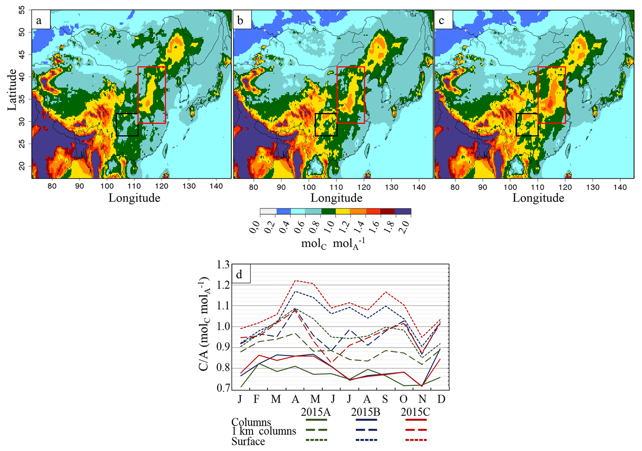
Figure 10Partial column (0–1 km) cation ∕ anion ratio (molC mol) over China for the simulations (a) 2015A, (b) 2015B and (c) 2015C and (d) monthly variation of C∕Aratio over eastern China. Full lines represent ratios derived from columns (up to 12 km), dashed lines represent ratios derived from the 0–1 km column and dotted lines represent ratios derived from surface concentrations. Black rectangles represent central China, and red rectangles northern China.
C∕Aratio two-dimensional distributions are shown in Fig. 10 for the 0–1 km column. The atmosphere is mainly cation-limited over eastern China in the 2015A initial scenario. As expected from the decrease in anion precursor emissions (i.e SO2 and NOx), the C∕Aratio is higher in the 2015C and 2015B simulations than in the 2015A simulation, as for example in the Sichuan Province and Chongqing municipality (black square in Fig. 10b) and northern China regions (red rectangle in Fig. 10c). Reductions of SO2 and NOx emissions led to a C∕Aratio increase and change in the limitation regime close to NH3(g) source areas (Fig. 10a and c). In the future, emission reductions for NH3 and anion precursors should reduce NH4NO3(p) and (NH4)2SO4(p) formation, reducing observed PM levels, which was already suggested in Fu et al. (2017). It should also be noted that cations such as Ca2+ or Mg2+ (from dust or anthropogenic emissions) are not included in CHIMERE chemistry. They could induce a bias in our analysis, underestimating the C∕Aratio. Nevertheless, we can reasonably assume here that the molar content is generally much higher than Ca2+ and Mg2+ content. A study by Li et al. (2013) with measurements in Beijing (from September 2006 to August 2007) shows that in winter, when the lowest concentrations are met, the content (about 0.5 µmol m−3) still exceeds 3 times the (Ca2+ + Mg2+) amount (about 0.15 µmol m−3). Another recent study measuring soluble ions of PM2.5 in Beijing shows a large excess of compared to Ca2+or Mg2+ in summer and winter 2014 (Chen et al., 2017). Still, not taking into account this chemistry for mineral cation species can lead to simulated cation-limited situations instead of a cation-excess situation for restricted times of the year and areas, when the ratio reaches values close to 1.
3.3 Time evolution of inorganic PM and precursor species between 2011 and 2015
The combined impacts of meteorology and emission reductions on gaseous and particulate species are shown in Fig. 11 using simulations 2011A, 2013C and 2015C including meteorology and updated emissions for the three corresponding years. The time evolution between 2011 and 2015 is qualitatively similar to that presented in the previous section for emission changes alone. The impact of changing meteorology is to damp the negative changes of pSNA (Sect. 3.1, Figs. 5 and S11 in the Supplement present two-dimensional distribution of pSNA changes) and the positive changes in NH3(g) due to emission reductions. As a result, in our simulations, NH3(g) columns increased by as much as +14 % in 2013 and by 41 % in 2015 over eastern China, as compared to 2011, combining both meteorological and emission changes.
3.4 Evaluation against PM2.5 surface measurements
The evolution of surface PM2.5, induced by changes in SO2 and NOx emissions in our simulations, is evaluated here against independent daily PM2.5 surface measurements. Scores for normalized bias, normalized RMSE (NRMSE), ratios of model and observed variability and Pearson correlation coefficients are displayed in Table 3. We used data from the U.S. Department of State Air Quality Monitoring Program over China (e.g. in Beijing, Chengdu, Guangzhou, Shanghai and Shenyang; http://www.stateair.net/, last access: 5 October 2018), for the years 2013 and 2015. For the year 2011, data are available only for Beijing, so this year was discarded. We present results for updated inventories (simulations 2013C and 2015C). We also present changes between simulations 2013A and 2015A and 2013C and 2015C in Table 3. The PM2.5 values measured in Chinese cities show large amplitudes, ranging from 0 to 500 µg m−3, and CHIMERE correctly represents both these amplitudes and the strong day-to-day variability of PM2.5 surface concentrations, as illustrated by good correlation coefficients (Pearson's coefficient averaging 0.7) between time series and a ratio of standard deviations close to unity (except for Shenyang; Table 3). Our 2013C and 2015C simulations overestimate average PM2.5 concentrations for four cities (Beijing, Shanghai, Guangzhou and Chengdu) and underestimate them for Shenyang (bias %). For the Beijing, Shanghai, Guangzhou and Chengdu stations, we observe a slight decrease of PM2.5 means (−4.3, −2.2, −1.1 and −11.5 µg m−3) between our reference simulations (2013A and 2015A) and simulations with modified inventories (2013C and 2015C). This means that updating the emissions improves agreement with observations by reducing biases and errors (NRMSE). We also find a slight decrease at Shenyang station (−1.1 µg m−3), making the already negative bias slightly worse. The strongest improvement is observed in Chengdu (central China), an area where inorganic PM mainly depends on sulfate and ammonium.
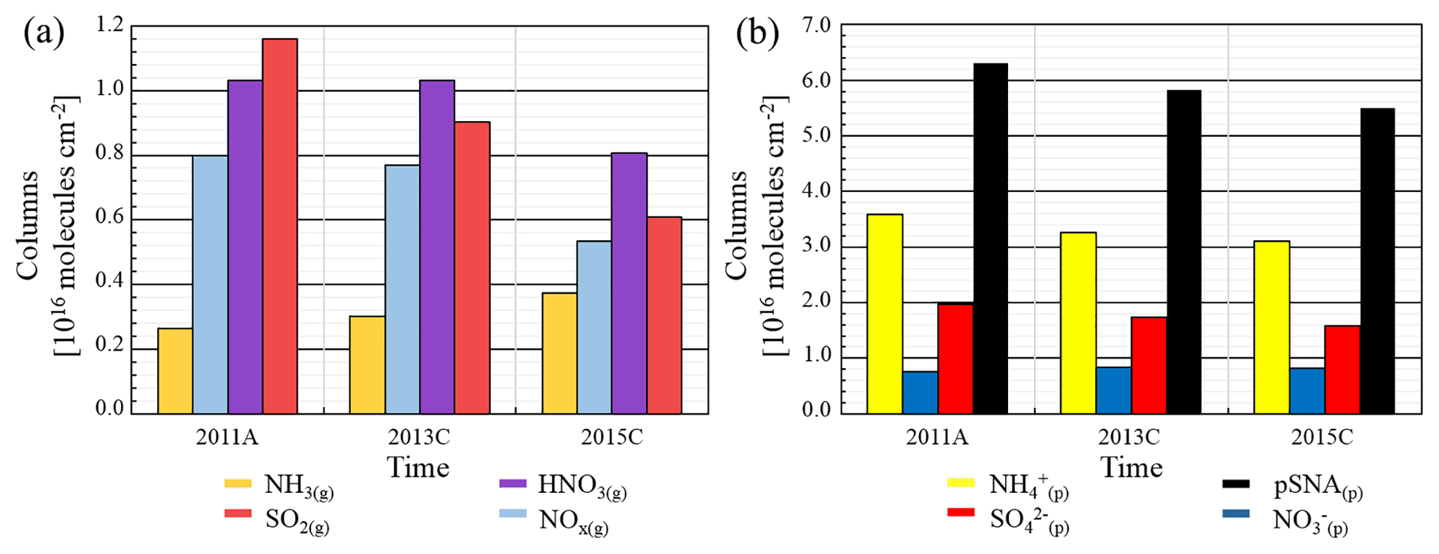
Figure 11(a) Evolution of NOx(g), SO2(g), NH3(g) and HNO3(g) tropospheric columns (molecules cm−2) for 2011A, 2013C and 2015C over the eastern China domain. (b) Evolution of , , and pSNA tropospheric columns (molecules cm−2) from 2011 to 2015 over the eastern China domain.
Table 3Daily PM2.5 comparison between model and measurements for 2013C and 2015C simulations. “Changes” corresponds to differences between 2013C and 2015C comparisons on the one hand and 2013A and 2015A on the other (i.e. biaschanges = biasC − biasA). Bias and NRMSE are normalized using the measurement mean. R corresponds to the Pearson correlation coefficient and n represents the number of available daily means.
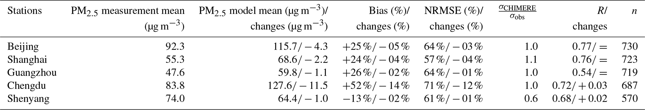
PM2.5 observations show a decrease from 2013 to 2015 for Beijing, Chengdu, Guangzhou and Shanghai of −19 %, −20 %, −30 % and −15 % respectively and an increase for Shenyang of +18 %. These changes are not fully reproduced by CHIMERE, possibly because emissions have been modified for NOx and SO2 only and not for organic or other inorganic species. In CHIMERE, PM2.5 decreases are calculated for Beijing and Chengdu (−3.6 % and −10 % respectively), no significant change is simulated for Guangzhou and increases are modelled for Shanghai and Shenyang (+12.5 % and +3.7 % respectively). All changes are calculated filtering simulation results according to the availability of measurements. The increase in Shenyang can be explained by a lack of data for a significant fraction of the sampling periods between 2013 and 2015 (229 d available against 341). In Shanghai, the modelled increase is not explained by PM2.5 inorganic components, which present a +1 % trend at surface, but is due to the effects of meteorological conditions on other PM2.5 components, which present larger increases.
3.5 Correspondences between CHIMERE simulations and IASI NH3(g) column observations
Data retrieved from the IASI instrument allow us to compare satellite observations to simulations and to verify the simulated trends. Figure 12 shows the spatial distributions of ammonia over China for IASI and CHIMERE for 2011, 2013 and 2015, presenting a similar spatial pattern and a good correlation ( over eastern China) and an acceptable daily correlation (). Nevertheless, simulations underestimate ammonia levels with a bias of −39 %, mainly because of the comparison over the sea area. As described above, IASI observations show a +65 % increase between 2011 and 2015. Interestingly, our model results between 2011A and 2015C, taking into account emission and meteorology changes, show a rather similar difference of +49 % of NH3(g) (when CHIMERE simulations are sampled on daily IASI observations' availability). For the intermediate year 2013, the IASI satellite observed a +15 % increase in NH3(g) columns, while CHIMERE simulations showed a +24 % increase in the 2013C scenario (again sampled on IASI observations). Conversely, simulations with unmodified emissions only show small changes for both years (+6 % in 2013A; −3 % in 2015A). Liu et al. (2018) estimated a +35 % NH3 column increase over the North China Plain, between 2011 and 2015, taking account of SO2 emissions decreases, a value close to our result for this case (+27 % between 2011A and 2015B). This suggests that the observed increase for ammonia by IASI can be explained to a large extent by changes in atmospheric chemistry induced by SO2 but also by NOx emission reductions, with less ammonium present within inorganic aerosol and more ammonia remaining in the gas phase.
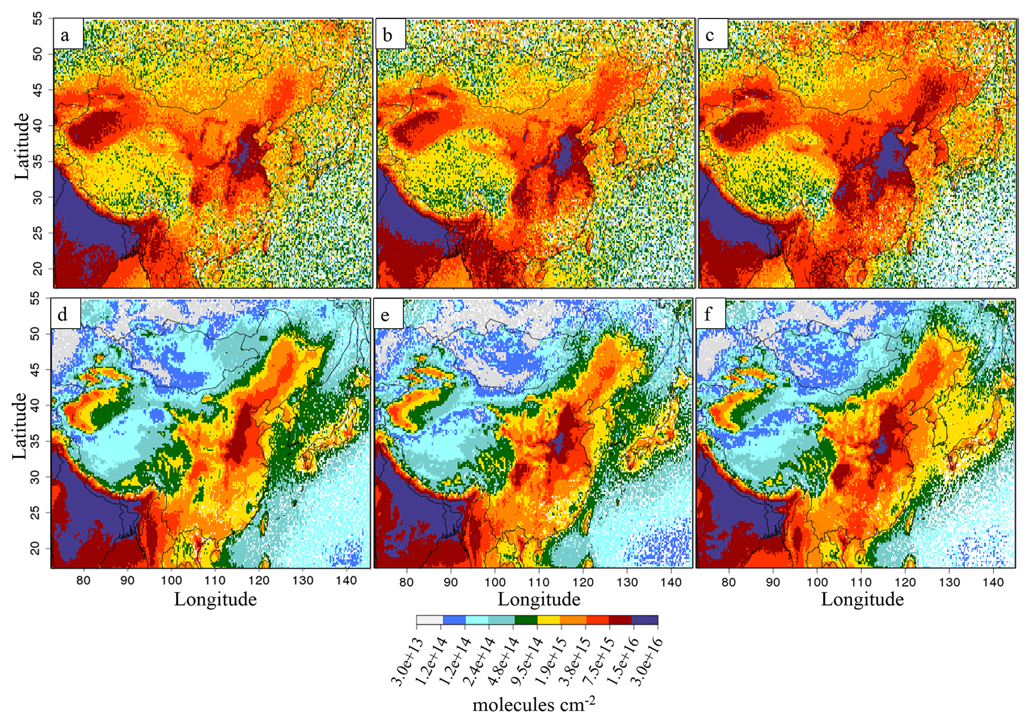
Figure 12Ammonia column evolution for IASI (a, b, c) and CHIMERE (d, e, f) in (a) 2011, (b) 2013, (c) 2015, (d) 2011A, (e) 2013C and (f) 2015C (molecules cm−2).
Sensitivity tests with the regional chemistry-transport model CHIMERE have been performed to understand the evolution of the NH3(g) atmospheric content over China, with an increase observed by IASI measurements over eastern China of +15 % between 2011 and 2013 and of +65 % between 2011 and 2015. One of the main results of this study is that the strong observed changes in the NH3(g) atmospheric content are mainly associated with a reduction of anthropogenic SO2 emissions and, to a lesser extent, with a reduction in anthropogenic NOx emissions and with interannual changes in meteorological conditions. With SO2 emissions reduced by 24 % between 2011 and 2013 and by 37.5 % between 2011 and 2015, and an additional NOx emission reduction of −21 % between 2011 and 2015, CHIMERE reproduces an increase in NH3(g) of +24 % between 2011 and 2013 and of +49 % between 2011 and 2015 (when filtering simulations according to IASI observations' availability). Also, it should be recalled that NH3 emissions have remained constant in our scenarios, as no precise information on NH3 emission changes was available to us, but Zhang et al. (2018) suggested a 7 % increase between 2011 and 2015, which could partly explain the difference between IASI and CHIMERE increases. SO2 and NOx emission reductions have been inferred from OMI satellite observations, so our study is to a large degree constrained by observations. Simulations then allow us to state that observed decreases in SO2 and NOx columns and increases in NH3 are mutually consistent. The cation / anion ratio shows an interesting height dependence. It is below unity for total columns, above unity for surface and near unity for the first kilometre of the atmosphere. The latter is probably most relevant for inorganic aerosol formation affecting air quality. Thus it appears that in addition to SO2 and NOx reductions, NH3 emission reductions would also be efficient to reduce inorganic aerosol formation. The reduction of SO2 and NOx emissions also leads to a decrease of inorganic pSNA production (−14 % in the tropospheric columns between 2011 and 2015), which is a major contributor to PM2.5 concentrations (about 50 % of surface PM2.5 and 33 % of column PM). A shift from sulfate to nitrate is simulated due to stronger SO2 reduction than NOx reduction, with more ammonia thus available for nitrate formation. Finally, based on our work, it appears that the changes in gaseous precursors must be updated each year to understand changes in PM. Current bottom-up inventories are not updated quickly enough. The method we used to derive inventories for 2013 and 2015 from satellite data provides an interesting first estimation but presents uncertainties when pollutants are transported or eliminated. It would be interesting to use inverse methods operating in synergy between regional CTM and atmospheric observations (i.e, DECSO; Mijling and Zhang, 2013) to better represent NOx and SO2 emissions. Inverse modelling systems could also be used to quantify NH3 emissions, as IASI space-based NH3 observations have shown considerable potential to reveal the high spatio-temporal variability of NH3 emissions (Fortems-Cheiney et al., 2016).
Data are available by contacting the author.
The supplement related to this article is available online at: https://doi.org/10.5194/acp-19-6701-2019-supplement.
ML and AFC designed the experiments, and ML carried them out. LC, CC, PFC and MVD were responsible for the satellite retrieval algorithm development and the processing of the IASI NH3 dataset. GS prepared meteorological and emission data. AFC prepared emission update and satellite data. ML adapted the model code, performed the simulations and prepared the paper. All authors contributed to the text and interpretation of the results and reviewed the paper.
The authors declare that they have no conflict of interest.
We acknowledge the free use of tropospheric NO2 column data from the OMI sensor from http://www.temis.nl/index.php (last access: 3 May 2019). The thesis of Mathieu Lachatre was funded by Sorbonne Universités, and this study was funded by PolEASIA ANR project under the allocation ANR-15-CE04-0005. This work was granted access to the HPC resources of TGCC under the allocation A0030107232 made by GENCI. PM2.5 measurements were provided by the U.S. Department of State Air Quality Monitoring Program, Mission China. IASI is a joint mission of EUMETSAT and the Centre National d'Études Spatiales (CNES, France). The authors acknowledge the Aeris data infrastructure (https://www.aeris-data.fr/, last access: 3 May 2019) for providing access to the IASI Level-2 NH3 data used in this study. The French scientists are grateful to CNES and Centre National de la Recherche Scientifique (CNRS) for financial support. The research in Belgium is also funded by the Belgian State Federal Office for Scientific, Technical and Cultural Affairs and the European Space Agency (ESA Prodex IASI Flow project).
This paper was edited by Kostas Tsigaridis and reviewed by two anonymous referees.
Ansari, A. S. and Pandis, S. N.: Prediction of multicomponent inorganic atmospheric aerosol behavior, Atmos. Environ., 33, 745–757, https://doi.org/10.1016/S1352-2310(98)00221-0, 1999. a
Banzhaf, S., Schaap, M., Wichink Kruit, R. J., Denier van der Gon, H. A. C., Stern, R., and Builtjes, P. J. H.: Impact of emission changes on secondary inorganic aerosol episodes across Germany, Atmos. Chem. Phys., 13, 11675–11693, https://doi.org/10.5194/acp-13-11675-2013, 2013. a
Bauer, S. E., Tsigaridis, K., and Miller, R.: Significant atmospheric aerosol pollution caused by world food cultivation, Geophys. Res. Lett., 43, 5394–5400, https://doi.org/10.1002/2016GL068354, 2016. a
Beirle, S., Boersma, K., Platt, U., Laurence, M., and Wagner, T.: Megacity emissions and lifetimes of nitrogen oxides probed from space, Science, 333, 1737–1739, https://doi.org/10.1002/2016GL068354, 2011. a
Chen, Q., Song, S., Stefan, H., Yuei-An, L., Zhu, W., and Jingyang, Z.: Assessment of ZTD derived from ECMWF/NCEP datawith GPS ZTD over China, GPS Solut., 15, 415–425, https://doi.org/10.1007/s10291-010-0200-x, 2010. a
Chen, R., Cheng, J., Lv, J., and Wu, L.: Comparison of chemical compositions in air particulate matter during summer and winter in Beijing, China, Environ. Geochem. Hlth., 39, 913–921, https://doi.org/10.1007/s10653-016-9862-9, 2017. a
Clarisse, L., Clerbaux, C., Dentener, F., Hurtmans, D., and Coheur, P. F.: Global ammonia distribution derived from infrared satellite observations, Nat. Geosci., 2, 479–483, https://doi.org/10.1038/ngeo551, 2009. a
Cohen, A. J., Brauer, M., Burnett, R., Anderson, H. R., Frostad, J., Estep, K., Balakrishnan, K., Brunekreef, B., Dandona, L., Dandona, R., Feigin, V., Freedman, G., Hubbell, B., Jobling, A., Kan, H., Knibbs, L., Liu, Y., Martin, R., Morawska, L., Pope, C. A., Shin, H., Straif, K., Shaddick, G., Thomas, M., van Dingenen, R., van Donkelaar, A., Vos, T., Murray, C. J., and Forouzanfar, M. H.: Estimates and 25-year trends of the global burden of disease attributable to ambient air pollution: an analysis of data from the Global Burden of Diseases Study 2015, The Lancet, 389, 1907–1918, https://doi.org/10.1016/S0140-6736(17)30505-6, 2017. a
de Foy, B., Lu, Z., and Streets, D.: Satellite NO2 retrievals suggest China has exceeded its NOx reduction goals from the twelfth Five-Year Plan, Sci. Rep.-UK, 6, 35912, https://doi.org/10.1038/srep35912, 2016. a
Ding, J., Miyazaki, K., van der A, R. J., Mijling, B., Kurokawa, J.-I., Cho, S., Janssens-Maenhout, G., Zhang, Q., Liu, F., and Levelt, P. F.: Intercomparison of NOx emission inventories over East Asia, Atmos. Chem. Phys., 17, 10125–10141, https://doi.org/10.5194/acp-17-10125-2017, 2017. a
Fortems-Cheiney, A., Dufour, G., Hamaoui-Laguel, L., Foret, G., Siour, G., Van Damme, M., Meleux, F., Coheur, P.-F., Clerbaux, C., Clarisse, L., Favez, O., Wallasch, M., and Beekmann, M.: Unaccounted variability in NH3 agricultural sources detected by IASI contributing to European spring haze episode, Geophys. Res. Lett., 43, 5475–5482, https://doi.org/10.1002/2016GL069361, 2016. a
Fu, X., Wang, S., Xing, J., Zhang, X., Wang, T., and Hao, J.: Increasing Ammonia Concentrations Reduce the Effectiveness of Particle Pollution Control Achieved via SO2 and NOX Emissions Reduction in East China, Environ. Sci. Tech. Let., 4, 221–227, https://doi.org/10.1021/acs.estlett.7b00143, 2017. a, b, c
Guenther, A., Karl, T., Harley, P., Wiedinmyer, C., Palmer, P. I., and Geron, C.: Estimates of global terrestrial isoprene emissions using MEGAN (Model of Emissions of Gases and Aerosols from Nature), Atmos. Chem. Phys., 6, 3181–3210, https://doi.org/10.5194/acp-6-3181-2006, 2006. a
Hedegaard, G. B., Brandt, J., Christensen, J. H., Frohn, L. M., Geels, C., Hansen, K. M., and Stendel, M.: Impacts of climate change on air pollution levels in the Northern Hemisphere with special focus on Europe and the Arctic, Atmos. Chem. Phys., 8, 3337–3367, https://doi.org/10.5194/acp-8-3337-2008, 2008. a
Hoyle, C. R., Fuchs, C., Järvinen, E., Saathoff, H., Dias, A., El Haddad, I., Gysel, M., Coburn, S. C., Tröstl, J., Bernhammer, A.-K., Bianchi, F., Breitenlechner, M., Corbin, J. C., Craven, J., Donahue, N. M., Duplissy, J., Ehrhart, S., Frege, C., Gordon, H., Höppel, N., Heinritzi, M., Kristensen, T. B., Molteni, U., Nichman, L., Pinterich, T., Prévôt, A. S. H., Simon, M., Slowik, J. G., Steiner, G., Tomé, A., Vogel, A. L., Volkamer, R., Wagner, A. C., Wagner, R., Wexler, A. S., Williamson, C., Winkler, P. M., Yan, C., Amorim, A., Dommen, J., Curtius, J., Gallagher, M. W., Flagan, R. C., Hansel, A., Kirkby, J., Kulmala, M., Möhler, O., Stratmann, F., Worsnop, D. R., and Baltensperger, U.: Aqueous phase oxidation of sulphur dioxide by ozone in cloud droplets, Atmos. Chem. Phys., 16, 1693–1712, https://doi.org/10.5194/acp-16-1693-2016, 2016. a
Huang, X., Song, Y., Li, M., Li, J., Huo, Q., Cai, X., Zhu, T., Hu, M., and Zhang, H.: A high-resolution ammonia emission inventory in China, Global Biogeochem. Cy., 26, GB1030, https://doi.org/10.1029/2011GB004161, 2012. a
Janssens-Maenhout, G., Crippa, M., Guizzardi, D., Dentener, F., Muntean, M., Pouliot, G., Keating, T., Zhang, Q., Kurokawa, J., Wankmüller, R., Denier van der Gon, H., Kuenen, J. J. P., Klimont, Z., Frost, G., Darras, S., Koffi, B., and Li, M.: HTAP_v2.2: a mosaic of regional and global emission grid maps for 2008 and 2010 to study hemispheric transport of air pollution, Atmos. Chem. Phys., 15, 11411–11432, https://doi.org/10.5194/acp-15-11411-2015, 2015. a
Jingjing, L., Jianping, H., Bin, C., Tian, Z., Hongru, Y., Hongchun, J., Zhongwei, H., and Beidou, Z.: Comparisons of PBL heights derived from CALIPSO and ECMWF reanalysis data over China, J. Quant. Spectrosc. Ra., 153, 102–112, https://doi.org/10.1016/j.jqsrt.2014.10.011, 2015. a
Kang, Y., Liu, M., Song, Y., Huang, X., Yao, H., Cai, X., Zhang, H., Kang, L., Liu, X., Yan, X., He, H., Zhang, Q., Shao, M., and Zhu, T.: High-resolution ammonia emissions inventories in China from 1980 to 2012, Atmos. Chem. Phys., 16, 2043–2058, https://doi.org/10.5194/acp-16-2043-2016, 2016. a, b
Koukouli, M. E., Theys, N., Ding, J., Zyrichidou, I., Mijling, B., Balis, D., and van der A, R. J.: Updated SO2 emission estimates over China using OMI/Aura observations, Atmos. Meas. Tech., 11, 1817–1832, https://doi.org/10.5194/amt-11-1817-2018, 2018. a
Kurokawa, J., Ohara, T., Morikawa, T., Hanayama, S., Janssens-Maenhout, G., Fukui, T., Kawashima, K., and Akimoto, H.: Emissions of air pollutants and greenhouse gases over Asian regions during 2000–2008: Regional Emission inventory in ASia (REAS) version 2, Atmos. Chem. Phys., 13, 11019–11058, https://doi.org/10.5194/acp-13-11019-2013, 2013. a
Landrigan, P. J., Fuller, R., Acosta, N. J., Adeyi, O., Arnold, R., Basu, N., Baldé, A. B., Bertollini, R., Bose-O'Reilly, S., Boufford, J. I., Breysse, P. N., Chiles, T., Mahidol, C., Coll-Seck, A. M., Cropper, M. L., Fobil, J., Fuster, V., Greenstone, M., Haines, A., Hanrahan, D., Hunter, D., Khare, M., Krupnick, A., Lanphear, B., Lohani, B., Martin, K., Mathiasen, K. V., McTeer, M. A., Murray, C. J., Ndahimananjara, J. D., Perera, F., Potočnik, J., Preker, A. S., Ramesh, J., Rockström, J., Salinas, C., Samson, L. D., Sandilya, K., Sly, P. D., Smith, K. R., Steiner, A., Stewart, R. B., Suk, W. A., van Schayck, O. C., Yadama, G. N., Yumkella, K., and Zhong, M.: The Lancet Commission on pollution and health, The Lancet, 391, 10119, https://doi.org/10.1016/S0140-6736(17)32345-0, 2017. a
Lelieveld, J., Evans, J. S., Fnais, M., Giannadaki, D., and Pozzer, A.: The contribution of outdoor air pollution sources to premature mortality on a global scale, Nature, 525, 367–371, https://doi.org/10.1038/nature15371, 2015. a
Li, X., Zhou, W., and Ouyang, Z.: Forty years of urban expansion in Beijing: What is the relative importance of physical, socioeconomic, and neighborhood factors?, Appl. Geogr., 38, 1–10, https://doi.org/10.1016/j.apgeog.2012.11.004, 2013. a
Liu, F., Beirle, S., Zhang, Q., van der A, R. J., Zheng, B., Tong, D., and He, K.: NOx emission trends over Chinese cities estimated from OMI observations during 2005 to 2015, Atmos. Chem. Phys., 17, 9261–9275, https://doi.org/10.5194/acp-17-9261-2017, 2017. a, b
Liu, M., Huang, X., Song, Y., Xu, T., Wang, S., Wu, Z., Hu, M., Zhang, L., Zhang, Q., Pan, Y., Liu, X., and Zhu, T.: Rapid SO2 emission reductions significantly increase tropospheric ammonia concentrations over the North China Plain, Atmos. Chem. Phys., 18, 17933–17943, https://doi.org/10.5194/acp-18-17933-2018, 2018. a, b, c
Mailler, S., Menut, L., Khvorostyanov, D., Valari, M., Couvidat, F., Siour, G., Turquety, S., Briant, R., Tuccella, P., Bessagnet, B., Colette, A., Létinois, L., Markakis, K., and Meleux, F.: CHIMERE-2017: from urban to hemispheric chemistry-transport modeling, Geosci. Model Dev., 10, 2397–2423, https://doi.org/10.5194/gmd-10-2397-2017, 2017. a
Menut, L., Bessagnet, B., Khvorostyanov, D., Beekmann, M., Blond, N., Colette, A., Coll, I., Curci, G., Foret, G., Hodzic, A., Mailler, S., Meleux, F., Monge, J.-L., Pison, I., Siour, G., Turquety, S., Valari, M., Vautard, R., and Vivanco, M. G.: CHIMERE 2013: a model for regional atmospheric composition modelling, Geosci. Model Dev., 6, 981–1028, https://doi.org/10.5194/gmd-6-981-2013, 2013. a
Mijling, B., van der A, R. J., and Zhang, Q.: Regional nitrogen oxides emission trends in East Asia observed from space, Atmos. Chem. Phys., 13, 12003–12012, https://doi.org/10.5194/acp-13-12003-2013, 2013. a, b
Nenes, A., Pilinis, C., and Pandis, S.: ISORROPIA: A new thermodynamic model for inorganic multicomponent atmospheric aerosols, Aquat. Geochem., 4, 123–152, 1998. a
Owens, R. G. and Hewson, T.: ECMWF Forecast User Guide, https://doi.org/10.21957/m1cs7h, 2018. a
Palmer, P. I., Abbot, D. S., Fu, T.-M., Jacob, D. J., Chance, K., Kurosu, T. P., Guenther, A., Wiedinmyer, C., Stanton, J. C., Pilling, M. J., Pressley, S. N., Lamb, B., and Sumner, A. L.: Quantifying the seasonal and interannual variability of North American isoprene emissions using satellite observations of the formaldehyde column, J. Geophys. Res.-Atmos., 111, D12315, https://doi.org/10.1029/2005JD006689, 2006. a
Paulot, F., Ginoux, P., Cooke, W. F., Donner, L. J., Fan, S., Lin, M.-Y., Mao, J., Naik, V., and Horowitz, L. W.: Sensitivity of nitrate aerosols to ammonia emissions and to nitrate chemistry: implications for present and future nitrate optical depth, Atmos. Chem. Phys., 16, 1459–1477, https://doi.org/10.5194/acp-16-1459-2016, 2016. a, b
Petetin, H., Sciare, J., Bressi, M., Gros, V., Rosso, A., Sanchez, O., Sarda-Estève, R., Petit, J.-E., and Beekmann, M.: Assessing the ammonium nitrate formation regime in the Paris megacity and its representation in the CHIMERE model, Atmos. Chem. Phys., 16, 10419–10440, https://doi.org/10.5194/acp-16-10419-2016, 2016. a
Pinder, R. W., Gilliland, A. B., and Dennis, R. L.: Environmental impact of atmospheric NH3 emissions under present and future conditions in the eastern United States, Geophys. Res. Lett., 35, L12808, https://doi.org/10.1029/2008GL033732, 2008. a
Pozzer, A., Tsimpidi, A. P., Karydis, V. A., de Meij, A., and Lelieveld, J.: Impact of agricultural emission reductions on fine-particulate matter and public health, Atmos. Chem. Phys., 17, 12813–12826, https://doi.org/10.5194/acp-17-12813-2017, 2017. a
Riddick, S., Ward, D., Hess, P., Mahowald, N., Massad, R., and Holland, E.: Estimate of changes in agricultural terrestrial nitrogen pathways and ammonia emissions from 1850 to present in the Community Earth System Model, Biogeosciences, 13, 3397–3426, https://doi.org/10.5194/bg-13-3397-2016, 2016. a
Schaap, M., van Loon, M., ten Brink, H. M., Dentener, F. J., and Builtjes, P. J. H.: Secondary inorganic aerosol simulations for Europe with special attention to nitrate, Atmos. Chem. Phys., 4, 857–874, https://doi.org/10.5194/acp-4-857-2004, 2004. a
Schiferl, L. D., Heald, C. L., Van Damme, M., Clarisse, L., Clerbaux, C., Coheur, P.-F., Nowak, J. B., Neuman, J. A., Herndon, S. C., Roscioli, J. R., and Eilerman, S. J.: Interannual variability of ammonia concentrations over the United States: sources and implications, Atmos. Chem. Phys., 16, 12305–12328, https://doi.org/10.5194/acp-16-12305-2016, 2016. a
Seinfeld, J. H. and Pandis, S. N.: Atmospheric Chemistry and Physics: From Air Pollution to Climate Change, 2nd edn., John Wiley & Sons, New York, USA, 2006. a, b
Stockwell, W. R. and Calvert, J. G.: The mechanism of the HO−SO2 reaction, Atmos. Environ., 17, 2231–2235, https://doi.org/10.1016/0004-6981(83)90220-2, 2016. a
Szopa, S., Foret, G., and Menut, L., and Cozic, A.: Impact of large scale circulation on European summer surface ozone: consequences for modeling, Atmos. Environ., 43, 1189–1195, https://doi.org/10.1016/j.atmosenv.2008.10.039, 2008. a
Van Damme, M., Whitburn, S., Clarisse, L., Clerbaux, C., Hurtmans, D., and Coheur, P.-F.: Version 2 of the IASI NH3 neural network retrieval algorithm: near-real-time and reanalysed datasets, Atmos. Meas. Tech., 10, 4905–4914, https://doi.org/10.5194/amt-10-4905-2017, 2017. a, b, c, d
Van Damme, M., Clarisse, L., Whitburn, S., Hadji-Lazaro, J., Hurtmans, D., Clerbaux, C., and Coheur, P.-F.: Industrial and agricultural ammonia point sources exposed, Nature, 564, 99–103, https://doi.org/10.1038/s41586-018-0747-1, 2018. a
Wang, Y., Zhang, Q. Q., He, K., Zhang, Q., and Chai, L.: Sulfate-nitrate-ammonium aerosols over China: response to 2000–2015 emission changes of sulfur dioxide, nitrogen oxides, and ammonia, Atmos. Chem. Phys., 13, 2635–2652, https://doi.org/10.5194/acp-13-2635-2013, 2013. a
Warner, J. X., Dickerson, R. R., Wei, Z., Strow, L. L., Wang, Y., and Liang, Q.: Increased atmospheric ammonia over the world's major agricultural areas detected from space, Geophys. Res. Lett., 44, 2875–2884, https://doi.org/10.1002/2016GL072305, 2017. a
Whitburn, S., Van Damme, M., Clarisse, L., Turquety, S., Clerbaux, C., and Coheur, P. F.: Doubling of annual ammonia emissions from the peat fires in Indonesia during the 2015 El Niño, Geophys. Res. Lett., 43, 11007–11014, https://doi.org/10.1002/2016GL070620, 2016. a
Wu, J., Kong, S., Wu, F., Cheng, Y., Zheng, S., Yan, Q., Zheng, H., Yang, G., Zheng, M., Liu, D., Zhao, D., and Qi, S.: Estimating the open biomass burning emissions in central and eastern China from 2003 to 2015 based on satellite observation, Atmos. Chem. Phys., 18, 11623–11646, https://doi.org/10.5194/acp-18-11623-2018, 2018. a
Zhang, L., Chen, Y., Zhao, Y., Henze, D. K., Zhu, L., Song, Y., Paulot, F., Liu, X., Pan, Y., Lin, Y., and Huang, B.: Agricultural ammonia emissions in China: reconciling bottom-up and top-down estimates, Atmos. Chem. Phys., 18, 339–355, https://doi.org/10.5194/acp-18-339-2018, 2018. a, b
Zheng, B., Tong, D., Li, M., Liu, F., Hong, C., Geng, G., Li, H., Li, X., Peng, L., Qi, J., Yan, L., Zhang, Y., Zhao, H., Zheng, Y., He, K., and Zhang, Q.: Trends in China's anthropogenic emissions since 2010 as the consequence of clean air actions, Atmos. Chem. Phys., 18, 14095–14111, https://doi.org/10.5194/acp-18-14095-2018, 2018. a, b