Analysis of sulfate aerosols over Austria: a case study

An increase in the sulfate aerosols observed in the period 1–6 April 2014 over Austria is analyzed using in situ measurements at an Austrian air quality background station, lidar measurements at the closest EARLINET stations around Austria, CAMS near-real-time data, and particle dispersion modeling using FLEXPART, a Lagrangian transport model. In situ measurements of SO₂, PM_2.5, PM₁₀, and O₃ were performed at the air quality background station Pillersdorf, Austria (EMEP station AT30, 48^∘43^′ N, 15^∘55^′ E). A CAMS aerosol mixing ratio analysis for Pillersdorf and the lidar stations Leipzig, Munich, Garmisch, and Bucharest indicates the presence of an event of aerosol transport, with sulfate and dust as principal components. For the sulfate layers identified at Pillersdorf from the CAMS analysis, backward- and forward-trajectory analyses were performed, associating lidar stations with the trajectories. The lidar measurements for the period corresponding to trajectory overpass of associated stations were analyzed, obtaining the aerosol layers, the optical properties, and the aerosol types. The potential sources of transported aerosols were determined for Pillersdorf and the lidar stations using the source–receptor sensitivity computed with FLEXPART, combined with the MACCity source inventory. A comparative analysis for Pillersdorf and the trajectory-associated lidar stations showed consistent aerosol layers, optical properties and types, and potential sources. A complex pattern of contributions to sulfate over Austria was found in this paper. For the lower layers (below 2000 m) of sulfate, it was found that central Europe was the main source of sulfate. Medium to smaller contributions come from sources in eastern Europe, northwest Africa, and the eastern US. For the middle-altitude layers (between 2000 and 5000 m), sources from central Europe (northern Italy, Serbia, Hungary) contribute with similar emissions. Northwest Africa and the eastern US also have important contributions. For the high-altitude layers (above 5000 m), the main contributions come from northwest Africa, but sources from the southern and eastern US also contribute significantly. No contributions from Europe are seen for these layers. The methodology used in this paper can be used as a general tool to correlate measurements at in situ stations and EARLINET lidar stations around these in situ stations.

1 Introduction

Sulfate is one of the major aerosol components for particles with a diameter smaller than 2.5 µm (PM_2.5) and for particles with a diameter smaller than 10 µm (PM₁₀). Other components of the particulate matter (PM) are organic carbon (OC), elemental carbon (EC), nitrate, ammonia, minerals, and sea salt. Sulfate normally accounts for about 10 % to 30 % of PM mass concentration (Stocker et al., 2013); worldwide in situ observations of refractory PM₁ chemical composition have shown that the sulfate contribution may reach more than 50 % of aerosol mass, depending on the location (Zhang et al., 2007). More details about the mass concentration of these aerosol components from various rural and urban sites in Europe are given in the IPCC AR5 report (Stocker et al., 2013). The anthropogenic sulfate is produced mainly by oxidation of sulfur dioxide (SO₂), or produced by aqueous phase reactions, where O₃ and hydrogen peroxide act as important oxidants (Seinfeld and Pandis, 2006), or by adsorption of SO₂ on solid particles and subsequent reaction with adsorbed oxygen; the exact mechanism depends on several atmospheric factors (solar radiation, presence of catalysts, NO_x, temperature, relative humidity, etc.). The adsorption is an important mechanism of sulfate production in the urban atmosphere. Soot (elemental carbon) particles and semiconductor metal oxide particulates from mineral dust (e.g., Fe₂O₃, TiO₂) are potential surfaces for this process (Dupart et al., 2012). The primary precursor for sulfate in the troposphere is SO₂ emitted (Solomon et al., 2007) from

• anthropogenic sources: a major contribution from combustion of fossil fuel (about 72 %) and a small contribution from biomass burning (about 2 %);

• natural sources: from dimethyl sulfide (DMS) emissions by marine phytoplankton (about 19 %) and from volcano eruptions (about 7 %).

A recent review of SO₂ sources worldwide can be found in Yang et al. (2017).

In addition to chemical processes, SO₂ is removed efficiently by dry deposition, while sulfate aerosol is removed from the atmosphere by wet deposition (Seinfeld and Pandis, 2006). Tropospheric sulfate, mostly in the accumulation mode, has a lifetime estimated at 1 week (AeroCom, 2018). The optical, physical, and chemical properties of the sulfate are well defined (Solomon et al., 2007). Sulfate particles have a cooling effect by light scattering (AeroCom, 2018; Stocker et al., 2013), they are very hygroscopic and therefore represent active cloud condensation nuclei, and they enhance absorption when deposited as a coating on elemental carbon. The direct radiative effects are strongly correlated to the emission sources, while the indirect effects are correlated to both emission sources and cloud cover (Déandreis et al., 2012; Yang et al., 2017). As a main component in the aerosols, sulfate can have an important contribution to the aerosol optical depth (AOD).

The purpose of this study is

• to assess the relation between the excess with respect to monthly averaged values observed in the in situ measurements of SO₂, O₃, PM_2.5, and PM₁₀ at the Austrian air quality background station Pillersdorf at the beginning of April 2014 with aerosol layers observed in lidar measurements at the closest EARLINET stations around Austria and with tropospheric sulfate aerosols as found in Copernicus Atmosphere Monitoring Service (CAMS) products (CAMS, 2018).

• to estimate the potential sources of sulfate aerosols.

The study is based on the synergy of the remote-sensing instruments from the European Aerosol Research Lidar Network (EARLINET) (Boesenberg et al., 2003); the ceilometer network of the German Meteorological Service (DWD) and in situ monitors, combined with CAMS products and the NATALI aerosol-typing model (Nicolae et al., 2018); and atmospheric transport modeling. The ground-based remote-sensing instruments and the CAMS products (assimilating satellite-based remote-sensing data) are used to determine the properties of long-range-transported aerosols and their vertical distribution. In situ measurements of PM and trace gases provide local concentrations at the surface and at specific heights in the troposphere. Details about data collection are given in Sect. 2.1.

The back-trajectory analysis relates the aerosol mass loading changes at a receptor location to spatially fixed sources, identifying the sources by a source–receptor matrix calculation (Seibert and Frank, 2004; Eckhardt et al., 2017). In this paper, the analysis of the trajectories has been performed with FLEXTRA (Stohl et al., 1995; FLEXTRA, 2018), while the estimation of the potential areas of aerosols' sources has been performed using the Lagrangian transport model FLEXPART (Stohl et al., 2005, Andreas Stohl et al., unpublished data, 2010). A detailed description of the processing of the collected data and the subsequent analysis is given in Sect. 2.3, while the results and the discussion are presented in Sect. 3.

The synergy of the in situ remote-sensing data and models was used in more atmospheric studies related to long-range-transported aerosols and estimation of their potential sources; see for example Papayannis et al. (2014) for dust, Nicolae et al. (2013) and Ansmann et al. (2018) for fires, Eckhardt et al. (2008) and Cazacu et al. (2012) for volcanic ash, and Sauvage et al. (2017), Chalbot et al. (2013), and Kaskaoutis et al. (2012) for anthropogenic aerosols. However, to the best of our knowledge, there have been no studies combining CAMS-based aerosol data with remote-sensing in situ measurements and transport models. The assimilation of ground-based remote-sensing measurements in CAMS is a long-term goal.

2 Methodology

The optical properties of the aerosol considered in this analysis are backscatter coefficients, extinction coefficients, volume depolarization ratio, particle depolarization ratio (PDepR), lidar ratio (LR), and Ångström exponent (AE).

In this paper, all times are given as UTC times, in the format HH:mm, HH being the hour and mm the minutes. The altitudes are given as ground-level altitudes (a.g.l.).

Whenever referring to measurements, the geographical name is used as an indicator for the station location (e.g., Pillersdorf means Pillersdorf site; Leipzig means Leipzig lidar station). In the plots, the stations are represented as Pillersdorf (red circle), Leipzig (green circle), Munich (magenta triangle), Garmisch (blue rhombus), and Bucharest (black square).

2.1 Data collection

The in situ measurement of SO₂, PM_2.5, PM₁₀, and O₃ were performed at the air quality background station Pillersdorf, Austria (EMEP station AT30, 48^∘43^′ N, 15^∘55^′ E) (Umweltbundesamt Austria, 2014). Pillersdorf (315 m) is located in hilly terrain in the northeastern part of Austria, around 60 km north from Vienna. The station is a part of the national background monitoring network and an EMEP background monitoring station. The surroundings are mostly forests and agricultural areas far from strong anthropogenic sources. Austria belongs to the midlatitude climate belt, in the transition between maritime and continental climate, and the weather is dominated mostly by traveling highs and lows. The station provides

• daily mean concentration and the maximum half-hour mean value per day for SO₂,

• daily mean concentration for PM_2.5 and PM₁₀,

• maximum value per day of hourly mean concentrations and maximum value per day of 8 h mean concentrations for O₃.

The SO₂ measurements are performed with a SO₂ analyzer, with a detection limit of 0.05 ppb, and a range up to 100 ppm. The PM_2.5 and PM₁₀ measurements are performed with an optical particle counter with a precision of 0.1 µg m⁻³. The O₃ measurements are performed with an ozone analyzer, with a detection limit of 0.4 ppb and a range of 0.05 to 200 ppm.

The EARLINET lidar stations (Wandinger et al., 2016) used for this study are Garmisch-Partenkirchen (47.47^∘ N, 11.06^∘ E), Leipzig (51.35^∘ N, 12.43^∘ E) (both stations located in Germany), and Bucharest (44.35^∘ N, 26.03^∘ E, Romania). The two DWD ceilometer stations used are located in Munich (48.20^∘ N, 11.45^∘ E) and Schneefernerhaus (47.42^∘ N, 10.98^∘ E). The following remote-sensing devices are deployed:

• high-spectral-resolution lidar (HSRL) (Wandinger et al., 2016), located at Garmisch-Partenkirchen, Germany;

• portable Raman multispectral lidar system Polly^XT (Engelmann et al., 2016), having eight channels including one water vapor channel and two depolarization channels, located at Leipzig, Germany;

• Raman multispectral lidar system (RALI) (Belegante et al., 2014), having seven channels including one water vapor channel and one depolarization channel, located at Bucharest, Romania;

• ceilometers (Wiegner and Geiß, 2012) at Munich and Schneefernerhaus, Germany.

The measurements were performed at the following wavelengths: 355, 532, and 1064 nm for the elastic channels; 387 and 607 nm for the Raman channels; and 532 nm for the depolarization channel. For HSRL, the 313 nm channel was used. For ceilometers, the 1064 nm channel was used.

The lidar and the ceilometer measurements provide the vertical distributions of aerosols, retrieved from the range corrected signal (RCS, the preprocessed lidar/ceilometer signal corrected with squared range), and the vertical distributions of aerosol polarization, if the instrument is equipped with a polarization channel.

For the remote-sensing sites Leipzig, Munich, and Bucharest, the column-integrated AOD measurements for various wavelengths were taken from the AERONET sun–sky photometer measurements, the AERONET instruments being collocated with the lidar stations.

In this paper, products from CAMS, the Copernicus Atmosphere Monitoring Service (CAMS, 2018) of the European Earth Observation program Copernicus were also used; it provides global reanalysis datasets for the period 2003–2012, and global near-real-time (NRT) datasets (Dee et al., 2011) for 2013 to present. These datasets were produced (Benedetti et al., 2009) using 4D-Var data assimilation in CY42R1 of ECMWF's Integrated Forecast System (IFS), with 60 hybrid sigma–pressure (model) levels in the vertical, with the top level at 0.1 hPa. Atmospheric data are available on these levels and they are also interpolated to 25 pressure, 10 potential temperature, and one potential vorticity level(s). “Surface or single level” data are also available.

For this analysis, the CAMS products for “model levels” and “surface level” from the NRT “Atmospheric Composition” dataset were selected for the times 00:00, 06:00, 12:00, and 18:00 for the analysis data and a step of 3 h for forecast data. The mixing ratios of dust, hydrophilic and hydrophobic black carbon, hydrophilic and hydrophobic organic matter, and sulfate were retrieved from the lowest 31 model levels, which cover the tropospheric altitudes; temperature and specific humidity were also retrieved for the same model levels. The logarithm of surface pressure was retrieved from the lowest model level, while the geopotential and aerosol optical depth (AOD) at 550 nm for total aerosol, black carbon, organic matter, dust, and sulfate were retrieved from the surface level.

2.2 Aerosol and atmospheric transport modeling

In this paper, the models FLEXPART and FLEXTRA were used for atmospheric transport modeling.

FLEXPART (FLEXible PARTicle dispersion model) is a Lagrangian particle dispersion model designed for calculating the long-range and mesoscale transport, diffusion, dry and wet deposition, and radioactive decay of air pollutants from point, line area, and volume sources. FLEXPART can be run in forward mode, simulating the transport and dispersion of emissions from given sources towards receptor points or producing gridded output concentration and deposition, or in backward mode from given receptors to produce source–receptor relationships with respect to a point source or gridded sources (Seibert and Frank, 2004). The model ingests ECMWF 3-D meteorological fields and solves the equations for transport, turbulent diffusions, and other relevant processes in a Lagrangian framework (Stohl et al., 1998; Pisso et al., 2019). The sensitivity of a receptor concentration to potential sources is obtained directly as the model output in the case of a backward run  (Seibert and Frank, 2004; Eckhardt et al., 2017).

FLEXTRA is a kinematic trajectory model. It simulates only the transport of air parcels by mean winds, ignoring turbulence and convection, and does not provide concentrations, deposition, etc.

For both models the ECMWF (European Centre for Medium-Range Weather Forecasts) ERA-Interim meteorological fields with a horizontal resolution of 0.5^∘ × 0.5^∘, the lowest 61 vertical levels (corresponding to pressure levels from the surface to 250 hPa) out of the 137 vertical levels, and a temporal resolution of 3 h were used. A sub-domain covering a part of the Northern Hemisphere (175^∘ W–60^∘ E, 0–90^∘ N), including Europe, a part of the Atlantic Ocean, North America, and a part of Africa was extracted as the “mother” domain.

For the determination of the aerosol optical properties for sites without lidar measurements, where the aerosol composition is determined from CAMS products, the aerosol model from Nicolae et al. (2018) was used, called in the following the NATALI aerosol model. Six classes of typical aerosol (called “pure aerosol” in the reference) were considered in this model: continental, continental polluted, dust, marine, smoke, and volcanic. In the model, the optical properties are computed for typical aerosols and for mixtures of two or three typical aerosols at fixed wavelengths 350, 550, and 1000 nm with the T-matrix method using light scattering on nonspherical particles (Mishchenko et al., 1996) for a lognormal distribution of homogeneous particles. The microphysical parameters (effective radius, standard deviation, and complex refractive indices) of the components, needed as input in the model, were taken from the GADS (Global Aerosol Data Set) database (Koepke et al., 1997).

For the comparison with optical properties obtained from lidar measurements, the optical properties computed in the model are rescaled to the lidar wavelengths (355, 532, and 1064 nm) using an AE equal to 1, as the values of model and lidar wavelengths are very close.

2.3 Data processing and analysis

2.3.1 Lidar and ceilometer data processing

The vertical profiles of the backscatter coefficients were determined using the Fernald–Klett method (Fernald, 1984; Klett, 1981) for remote-sensing instruments with only elastic channels. For instruments with elastic and Raman channels, the backscatter and the extinction coefficients were determined using the combined method (Ansmann et al., 1992). The PDepR was computed using the volume depolarization ratio and the backscatter coefficients (Freudenthaler, 2016). The AE is computed from the extinction coefficients for the wavelengths 532 and 355 nm.

The LR was computed as the ratio of the extinction coefficient to backscatter coefficient. For ceilometers, lidars with only elastic channels, and lidar measurements during the day (when only backscatter coefficients can be retrieved), the value of the LR was taken from the NATALI aerosol model, which gives an estimate of the LR for 14 aerosol types. The values for 532 nm used in this paper are 23±10 sr for marine, 40±8 sr for dust, 68±6 sr for continental, 52±2 sr for continental polluted, 53±5 sr for polluted dust, 64±8 sr for smoke, and 46±10 sr for mixed dust.

The aerosol layers are identified from the lidar measurements with the gradient method, applied to the RCS profiles (Belegante et al., 2014; Nicolae et al., 2018). The gradient method is based on the identification of the peaks and valleys from the first derivative applied to the vertical profiles. If two consecutive layers are very close (less than 100 m), these layers are merged into one layer. Also, if the signal-to-noise ratio in the layer is lower than a threshold (here set to 5), the layer is discarded.

The aerosol type is determined from the lidar measurements using the NATALI typing algorithm, described in Nicolae et al. (2018).

2.3.2 CAMS product processing

The values of the CAMS products (mixing ratios, temperature, specific humidity, etc.) for a given location were computed by interpolating the gridded CAMS values, using the inverse weighting distance interpolation.

The air density and the altitude specific to the model levels were computed according to CY42R1 from IFS documentation (Benedetti et al., 2009).

2.3.3 Data analysis

The concentrations of SO₂, PM_2.5, PM₁₀, and O₃ measured in situ at the air quality background station Pillersdorf were analyzed for sliding periods of 1 month to identify excesses with respect to the measured average values. If a significant excess is identified (values exceed the averaged values by 50 % for 30 d), the corresponding period is analyzed in detail, also using CAMS products at the in situ station and measurements and CAMS products at the closest lidar stations around the in situ station. For spring 2014, a period with a significant excess was identified in the time interval 15 March–14 April, which is presented in this paper.

The CAMS products are retrieved for the in situ site. The time series of mixing ratios of sulfate, dust, organic matter, and total aerosols are then analyzed for the same period as the in situ data. If one of the aerosol components has no significant contribution to the aerosol concentration, this component can be neglected in the subsequent analysis of the aerosol. The time series are also retrieved for the lidar stations around the in situ site.

To assess if the excess is caused by a local event or long- or medium-range-transported aerosol is involved, a qualitative analysis of the in situ concentration measurements and the time series of mixing ratios at the in situ station and at the lidar stations around the in situ station is performed. If the event is present only at the in situ station, we can assume that it is a local event. If the event is seen at some of the lidar stations around the in situ site, the event has contributions from an aerosol transport event.

The layers for the event at the in situ site are then determined by applying the same gradient method as for lidar data processing, but applied to the altitude profiles of aerosol concentrations. The concentrations are computed by multiplying the CAMS mixing ratios and the air density.

A statistical analysis of trajectories is then performed for each layer identified at the in situ site. Three-dimensional kinematic hourly trajectories are computed with the FLEXTRA model, run in backward mode for a transport time of 10–20 d (typical for long-range transport) and in forward mode for a few days for several receptor altitudes between 1500 and 7000 m. Due to the turbulence in the planetary boundary layer, trajectories below 1500 m are usually not included in the analysis, as mostly local trajectories. During the period under investigation, with low wind speeds and mostly clear skies, the boundary-layer height varied at Pillersdorf from less than 100 m at night to about 1500 m in the afternoon.

A trajectory is associated with a lidar station if the projection of the trajectory on the Earth's surface intersects a 0.5^∘ × 0.5^∘ cell centered on the lidar station location. The altitude of the trajectory and the time the trajectory overpasses the lidar cell are the altitude and time of the FLEXTRA trajectory at the corresponding location.

If a trajectory overpasses a lidar station, the lidar measurements for the overpass time are analyzed. The aerosol layers are identified with the same method (Belegante et al., 2014) as for an in situ station, applied to the RCS profiles. The optical properties are computed for each identified aerosol layer, as described in Sect. 2.3. The type of the aerosol is determined from the optical properties using the NATALI typing algorithm. The aerosol concentrations are also computed for each layer, using the method described in Mamouri and Ansmann (2017). For each layer, the sulfate fraction (SF) is computed as the ratio of sulfate concentration to total aerosol concentration.

The layers determined from lidar measurements are then compared with the altitude of the trajectories overpassing the lidar station. If the altitude matches a layer within a reasonable distance, the trajectory is associated with the layer. The matching distance is defined as 2σ_lidar, where σ_lidar is the effective spatial resolution of the lidar, typically of the order of ∼60 m.

The source–receptor sensitivity (SRS) is then computed for each layer identified in the sulfate profile at the in situ station using FLEXPART with sulfate as a passive tracer. The receptor is set to the location of the in situ station, at the altitude determined for that layer and the corresponding event time interval. Sources are considered to be situated between 0 and 100 m. Wet and dry deposition are taken into account in the computation. Combining the source–receptor sensitivity with emission inventories, the relative distributions of SO₂ sources for the corresponding sulfate layer are computed. In this study, the MACCity anthropogenic SO₂ emission inventories from the Emissions of atmospheric Compounds & Compilation of Ancillary Data (ECCAD) emission database (Darras et al., 2018) were used.

A cross-check of sulfate concentrations from lidar measurements, CAMS sulfate products, and FLEXPART is carried out for the layers at the lidar stations associated with the layers at the in situ station. One expects the values from the three methods to be in agreement.

The optical properties of the aerosol from each layer at the in situ station are then computed according to Sect. 2.2 and compared with the optical properties of the aerosol from the layers at the lidar stations associated with the layers at the in situ station. The optical properties determined at both sites have to be compatible, up to the changes due to the transport from one site to the other. The compatibility is also cross-checked for the type of aerosols at both stations, where the type is determined using the NATALI aerosol model at the in situ site and the NATALI typing algorithm at the lidar station.

3 Results and discussion

3.1 Results

The in situ measurements of SO₂, O₃, PM_2.5, and PM₁₀ concentrations recorded at Pillersdorf for the period 15 March–14 April 2014 (Umweltbundesamt Austria, 2014) are shown in Fig. 1, together with the averaged values for this period (dotted line). An excess with respect to the averaged values is observed for all measurements in the period 1–6 April: 66 % for SO₂, 11 % for O₃, and 90 % for PM_2.5 and PM₁₀. If the excess period is excluded from the calculation of the average values, the excess increases to 100 % for SO₂, 14 % for O₃, 153 % for PM_2.5, and 143 % for PM₁₀.

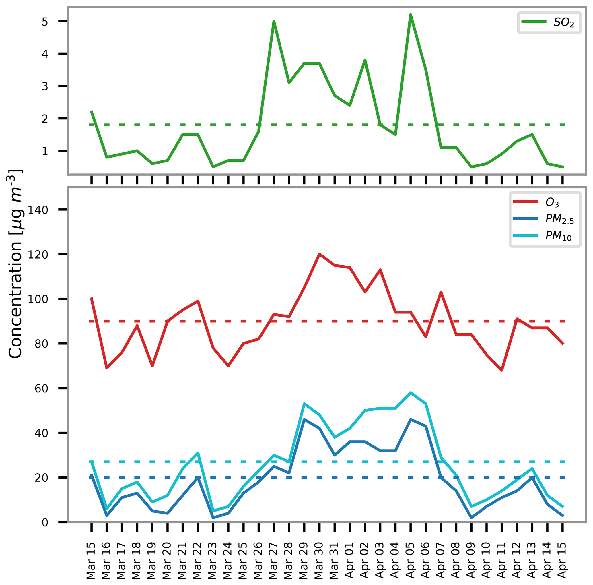
Figure 1 In situ SO₂, O₃, PM_2.5, and PM₁₀ concentrations measured at Pillersdorf, Austria (EMEP station AT30, 48^∘43^′ N, 15^∘55^′ E). The dotted lines represent the averaged values for the plotted period.

The time series of aerosol mixing ratios from CAMS near-real-time data for Pillersdorf are shown for the same period in Fig. 2 for “total aerosols” (sum of all species defined in CAMS data), for sulfate, and for dust. One observes a sulfate increase with a peak on 2 April, and a second, less pronounced peak on 4 April. The aerosol mixture is dominated by dust and sulfate, as can be seen by qualitatively comparing the total, sulfate, and dust distributions.

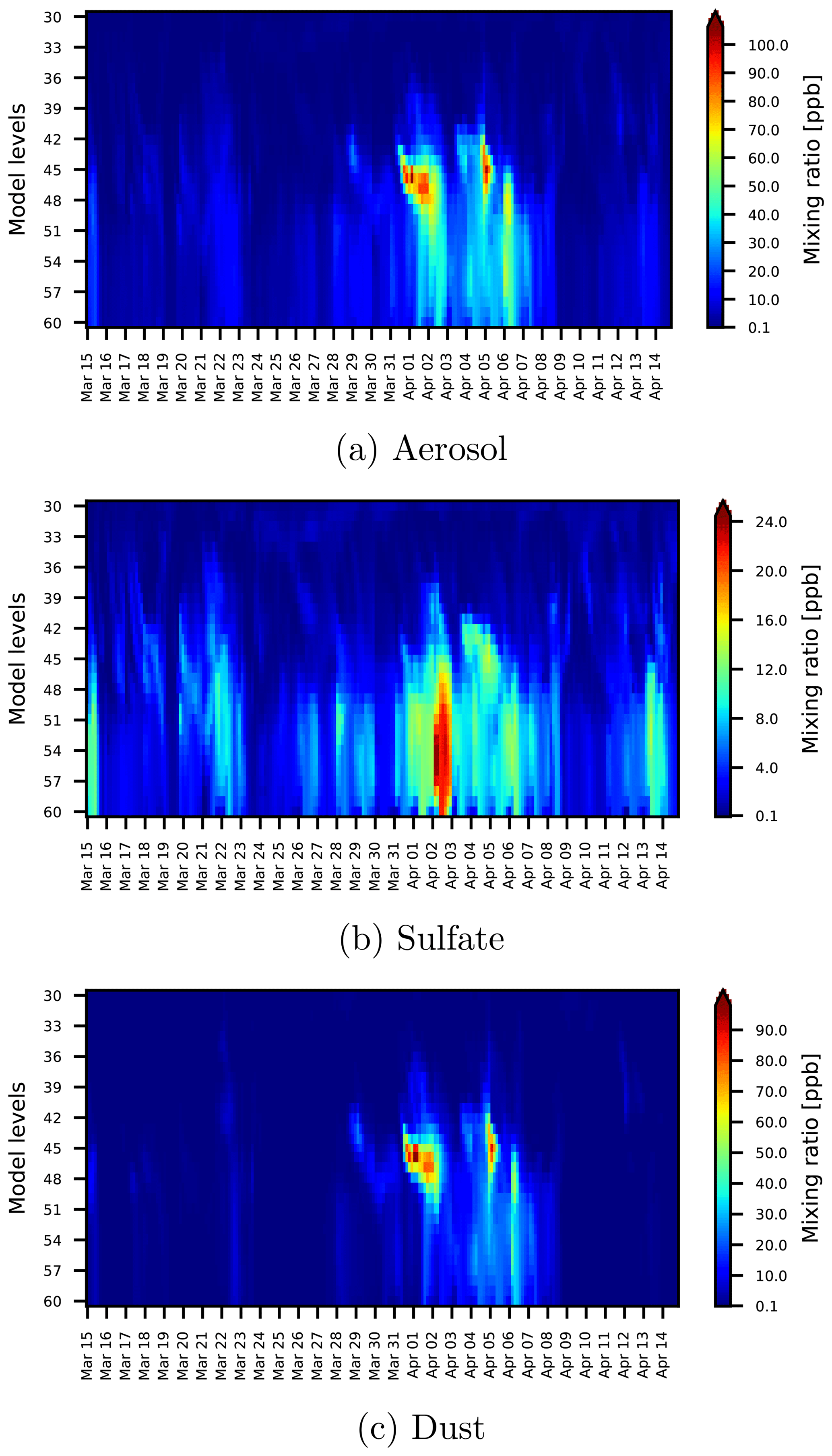
Figure 2 Time series of CAMS mixing ratios for total aerosol (a), sulfate (b), and dust (c), Pillersdorf, 15 March–14 April 2014.

Similar distributions, also retrieved from CAMS near-real-time data, are observed for the lidar stations around Pillersdorf, as shown in Fig. 3 for Munich, Leipzig, and Bucharest. From these distributions, one can infer the presence of an event of sulfate transport over Europe.

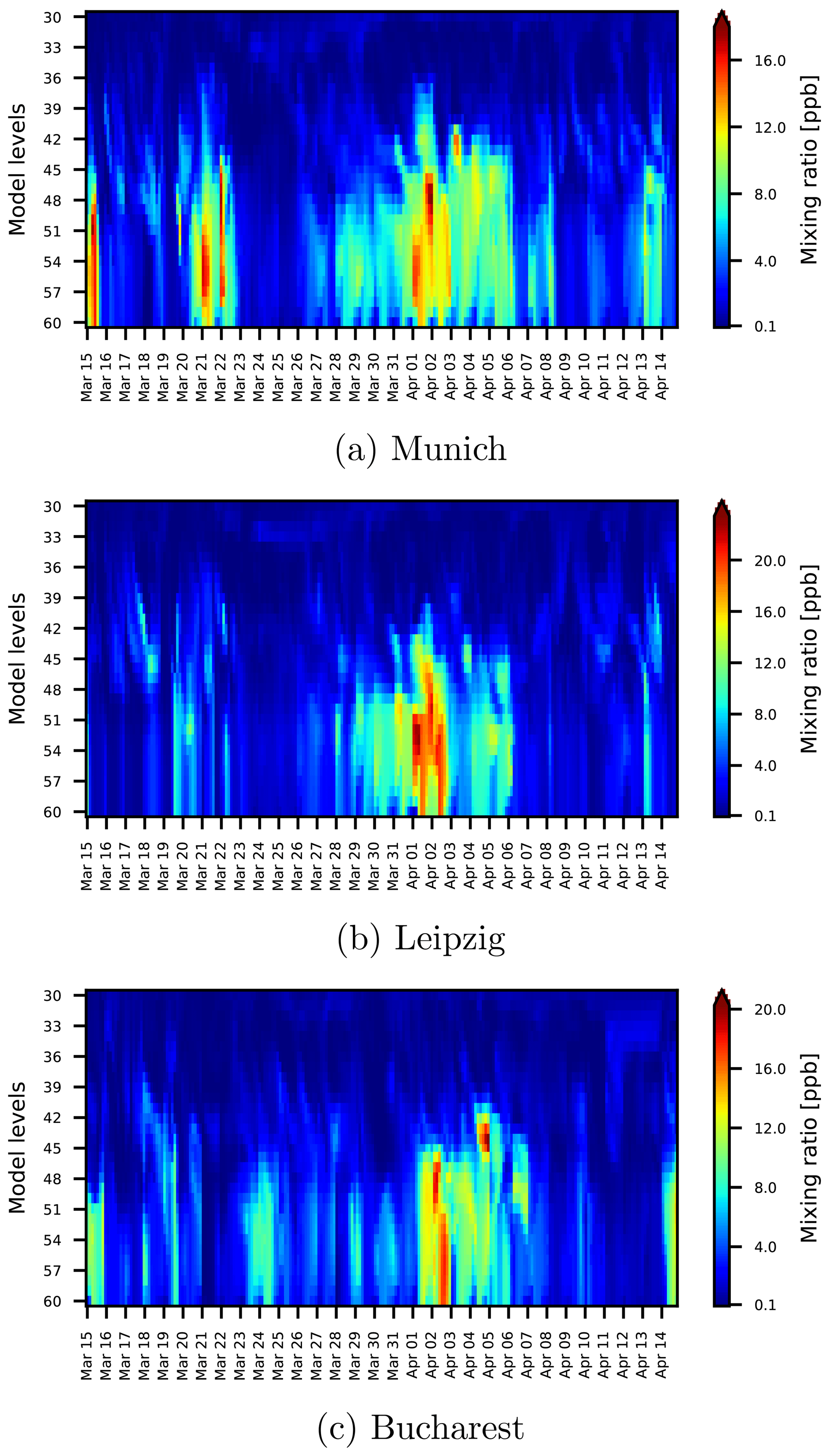
Figure 3 Time series of CAMS mixing ratios for sulfate for Munich (a), Leipzig (b), and Bucharest (c), 15 March–14 April 2014.

The vertical profiles of sulfate, dust, and total aerosol concentrations are shown in Fig. 4 for Pillersdorf, 2 April. The sulfate layers, identified with the gradient method, are shown as the gray area in the same figure.

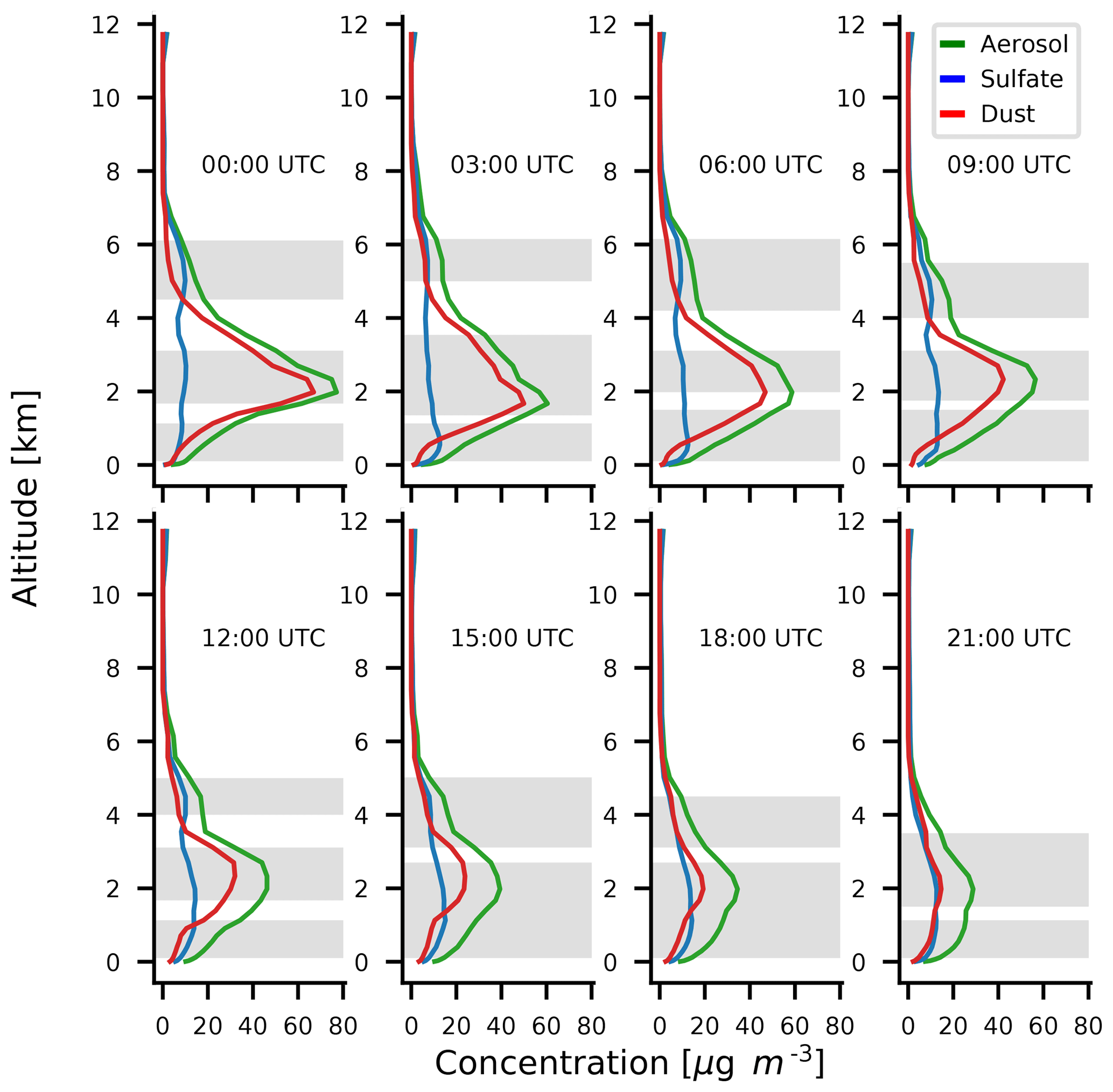
Figure 4 CAMS total aerosol, sulfate, and dust profiles for 2 April 2014, Pillersdorf. The gray area represents the identified sulfate layers. Altitudes are given in kilometers above ground level. Local time is UTC+2.

For 2 April, from 00:00 to 12:00, sulfate layers mixed with dust are well defined between 2 and 3 km and between 4 and 6 km. During the day, the layers descend slowly and disperse, such that they mix with dust and the aerosols from the planetary boundary layer. This can also be seen from the concentration profile of total aerosol, which also shows a similar structure, indicating a common transport path of sulfate and dust as polluted dust nearby Pillersdorf. The evolution of the sulfate and dust layers during the day is correlated with the increase in SO₂ and PM_2.5 concentrations measured in situ, while the evolution of the dust layers is correlated with the increase in the PM₁₀ concentration.

For the layers identified above, the back trajectories of the aerosols were computed with FLEXTRA, starting from Pillersdorf at the time corresponding to the aerosol profiles for a backward period of 12 d. As mentioned before, trajectories below 1500 m are not computed, due to turbulence in the planetary boundary layer.

For 2 April, they are shown in Fig. 5 for 00:00, 06:00, 12:00, and 18:00. From the trajectory analysis, the time, and the altitude of the trajectories passing over the lidar stations were determined. The station, the time and the altitude are shown in the lower plots of each panel.

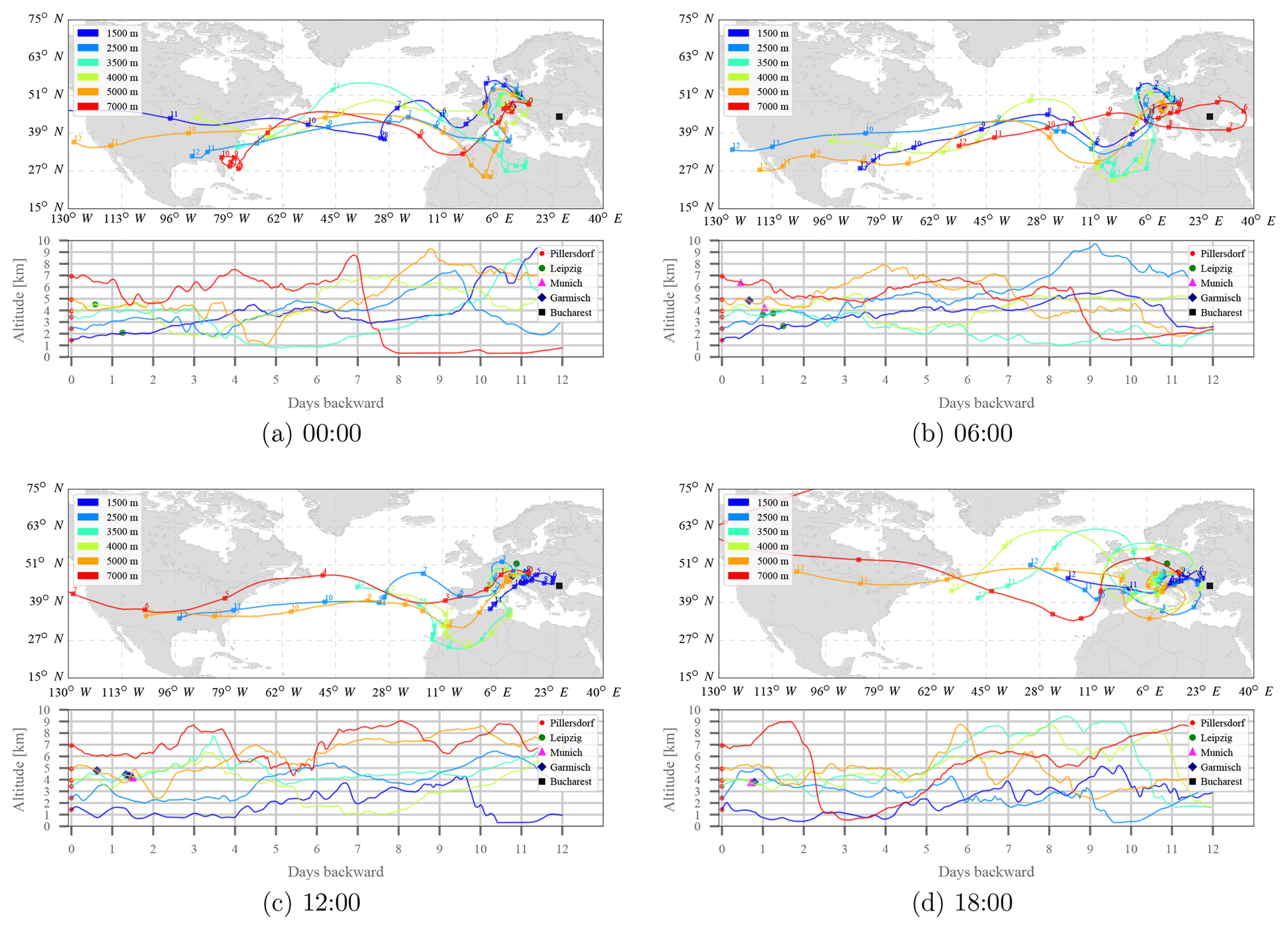
Figure 5 Pattern of back trajectories (upper plot of each panel) and their altitude profile, including overpassed lidar stations (lower plot of each panel) for Pillersdorf, 2 April 2014 at 00:00 (a), 06:00 (b), 12:00 (c), and 18:00 (d).

The aerosol layers identified at Pillersdorf were transported further. Some of the layers pass over the lidar station from Bucharest. Their trajectories were analyzed running FLEXTRA in forward mode for 3 d, starting from Pillersdorf. Figure 6 shows the forward trajectories for 2 April, 06:00, which pass over the Bucharest lidar station on 3 April.

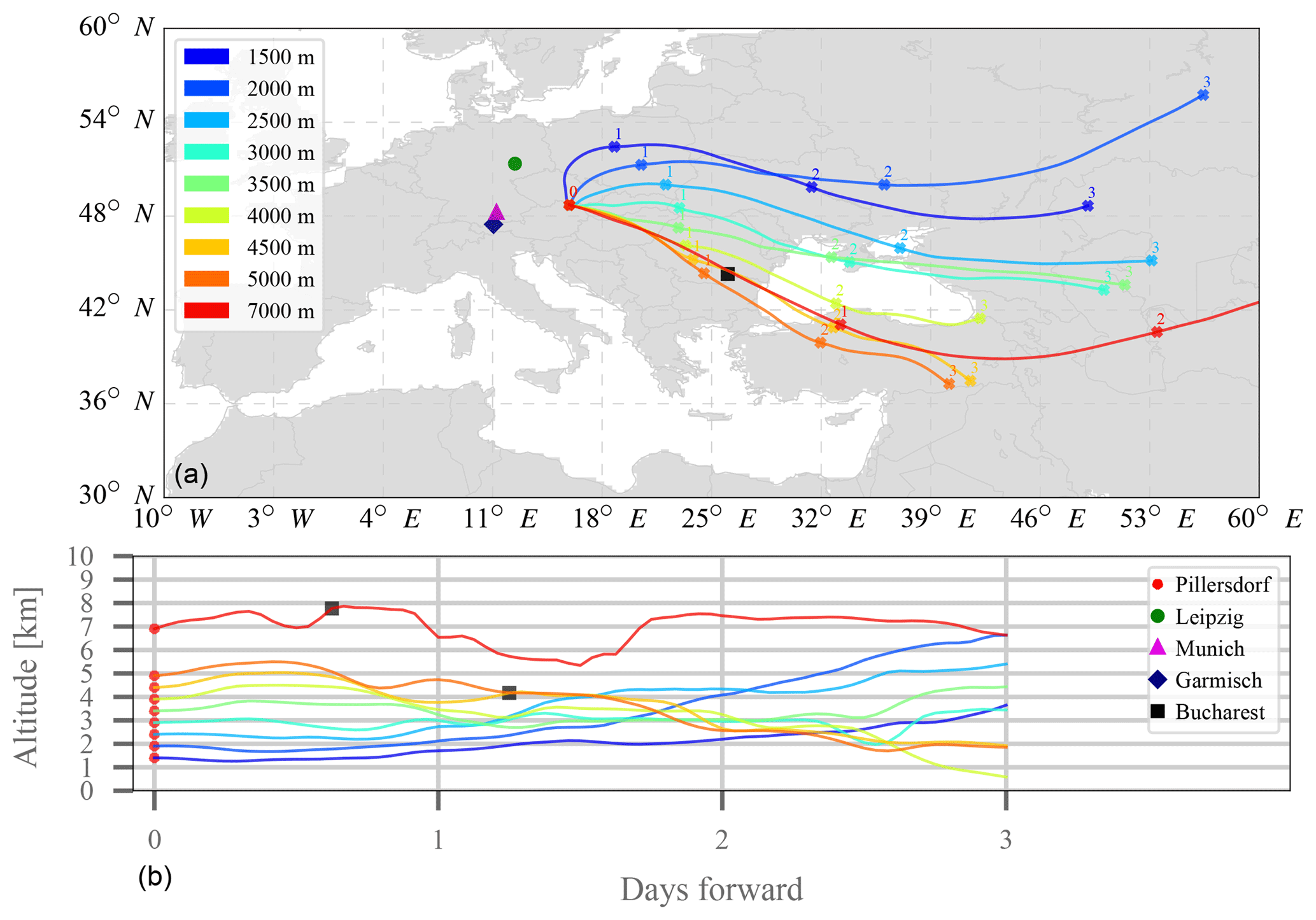
Figure 6 Pattern of forward trajectories (a) and their altitude profile, including overpassed lidar stations (b) for Pillersdorf, 2 April 2014, 06:00.

The lidar measurements for the stations overpassed by the trajectories determined from the backward and forward analyses are presented as range-corrected signal time series (RCS) in Figs. 7 and 8 and for the event on 2 April in Pillersdorf.

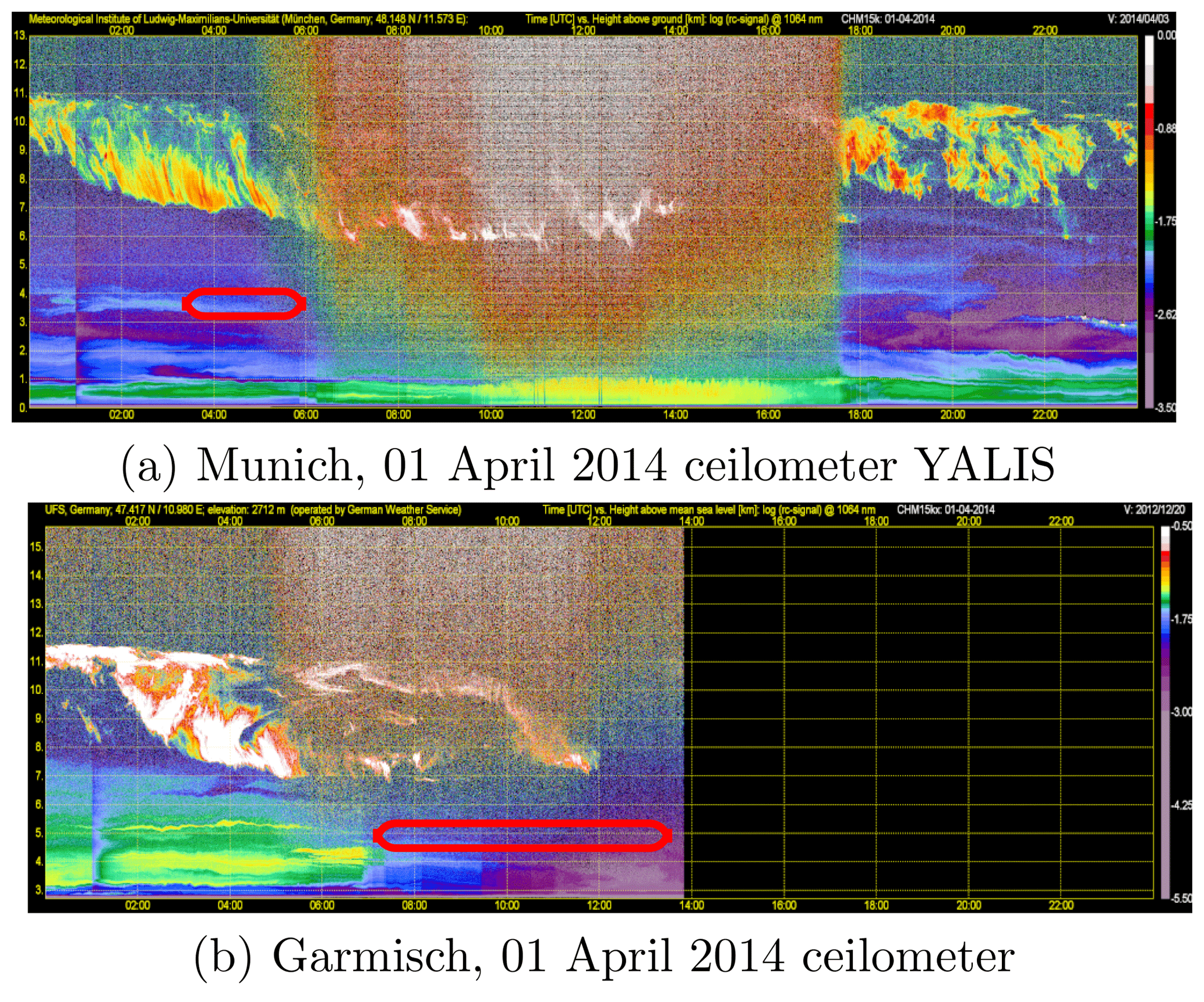
Figure 7 Logarithm of the range-corrected signal at 1064 nm, 24 h, for the Munich (a) and Garmisch (b) stations. The red boxes represent the identified layers.

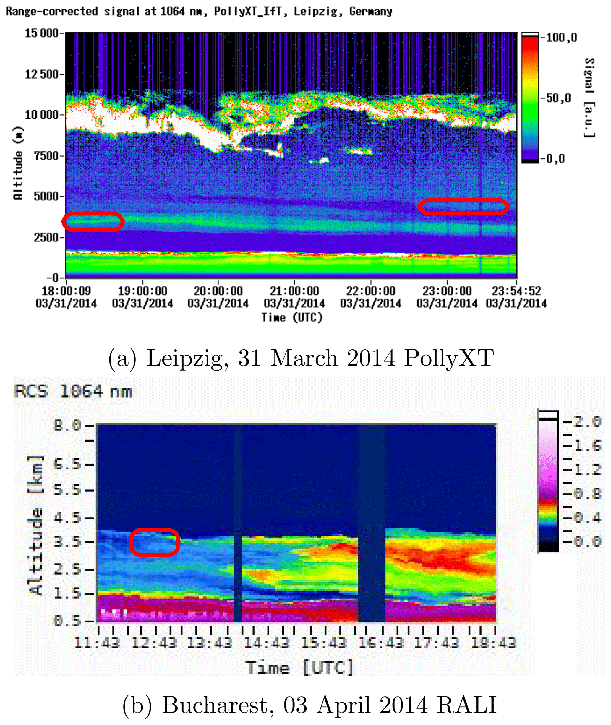
Figure 8 Range-corrected signal at 1064 nm for the Leipzig (a) and Bucharest (b) stations. The red boxes represent the identified layers.

Aerosol layers, their optical properties, and the concentration were determined from the lidar measurements following the methodology described in Sect. 2. The layers identified are marked on the corresponding RCS plot.

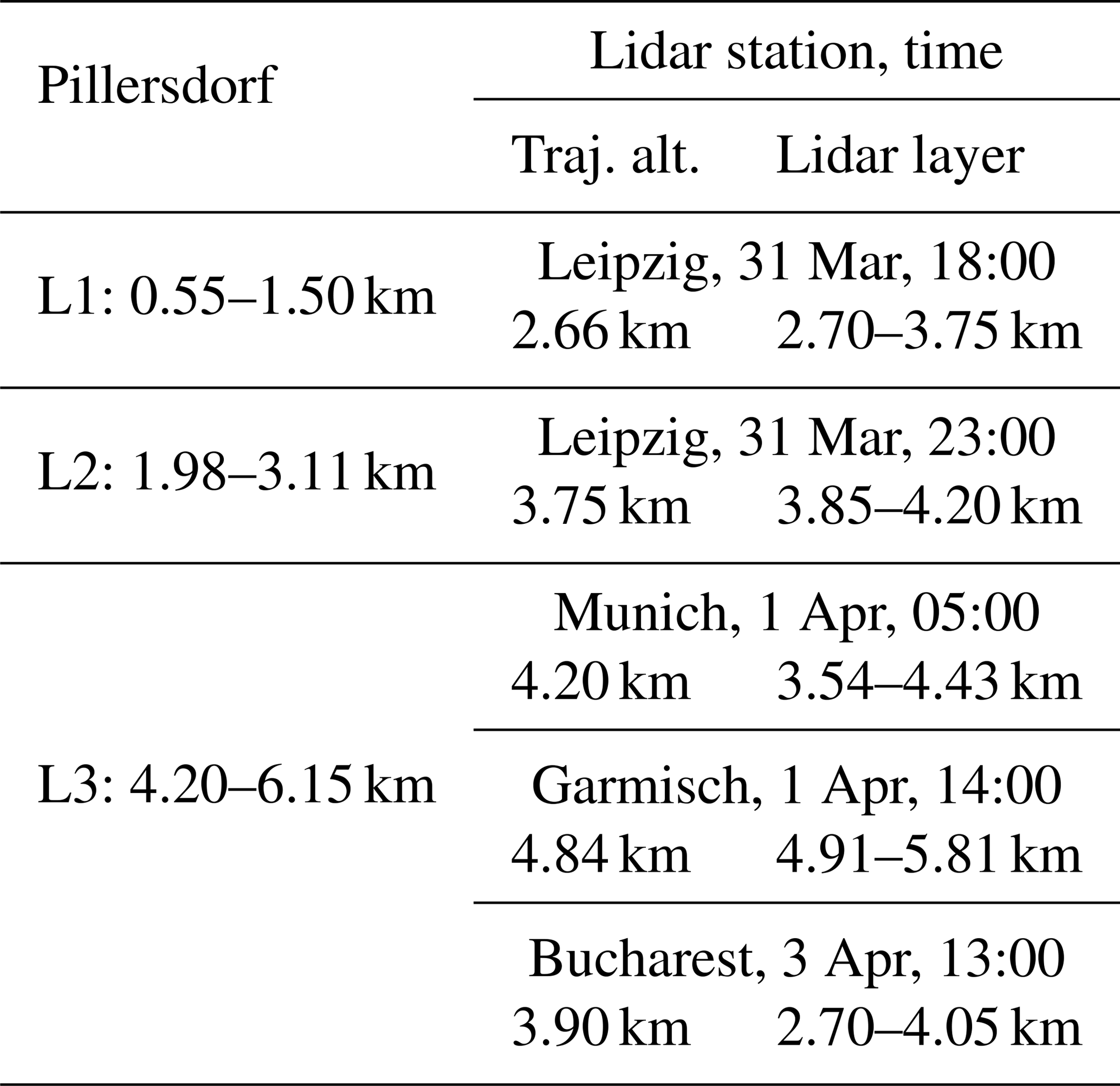
The association of the layers identified from lidar measurements with the altitude of the backward or forward trajectories over the stations corresponding to the layers identified in Pillersdorf was performed for all eight concentration profiles measured (see Fig. 4 for 2 April and Fig. 13 for 4 April). The association for trajectories from 2 April at 06:00 is presented in Table 1. The trajectory altitude (Traj. alt.) in the table represents the altitude of the trajectory when overpassing the lidar station. The corresponding layers are also marked in the RCS plots (red box).

Table 1 Association of layers from lidar measurements with layers and trajectories computed for Pillersdorf, 02 April 2014, 06:00.

The source–receptor sensitivity was computed for each layer identified in the sulfate profiles at Pillersdorf; the column-integrated source–receptor sensitivity was also computed. Figure 9 shows the corresponding distributions for the layers L1, L2, and L3 and total column from 2 April, 06:00.

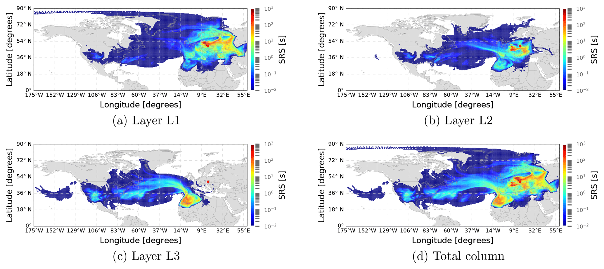
Figure 9 Source–receptor sensitivity for layers L1 (a), L2 (b), and L3 (c) and total column (d), Pillersdorf, 2 April, 06:00.

For each layer, the relative distribution of the SO₂ sources was computed from the source–receptor sensitivity and the source inventory MACCity. Figure 10a shows the distribution for layer L1 at Pillersdorf, 2 April, 06:00, while Fig. 10b shows the distribution for the corresponding layer at Leipzig, 31 March, 18:00. To evaluate the local distribution of sources near Pillersdorf, a zoomed view of the SO₂ relative distribution is shown in Fig. 10c for the sub-domain covering a part of the Europe, centered in Austria (10^∘ W–40^∘ E, 35–60^∘ N). Similar distributions are shown for layer L2 in Pillersdorf in Fig. 11a, with a corresponding layer in Leipzig (31 March, 23:00), shown in Fig. 11b, and the zoomed view for Pillersdorf in Fig. 11c. For layer L3 at Pillersdorf, the distribution is shown in Fig. 12a, with associated layers in Munich (1 April, 05:00), Garmisch (1 April, 14:00 – not shown as very close to Munich), and Bucharest (3 April, 13:00) shown in Fig. 12b and c, and a zoomed view for Pillersdorf in Fig. 12d.

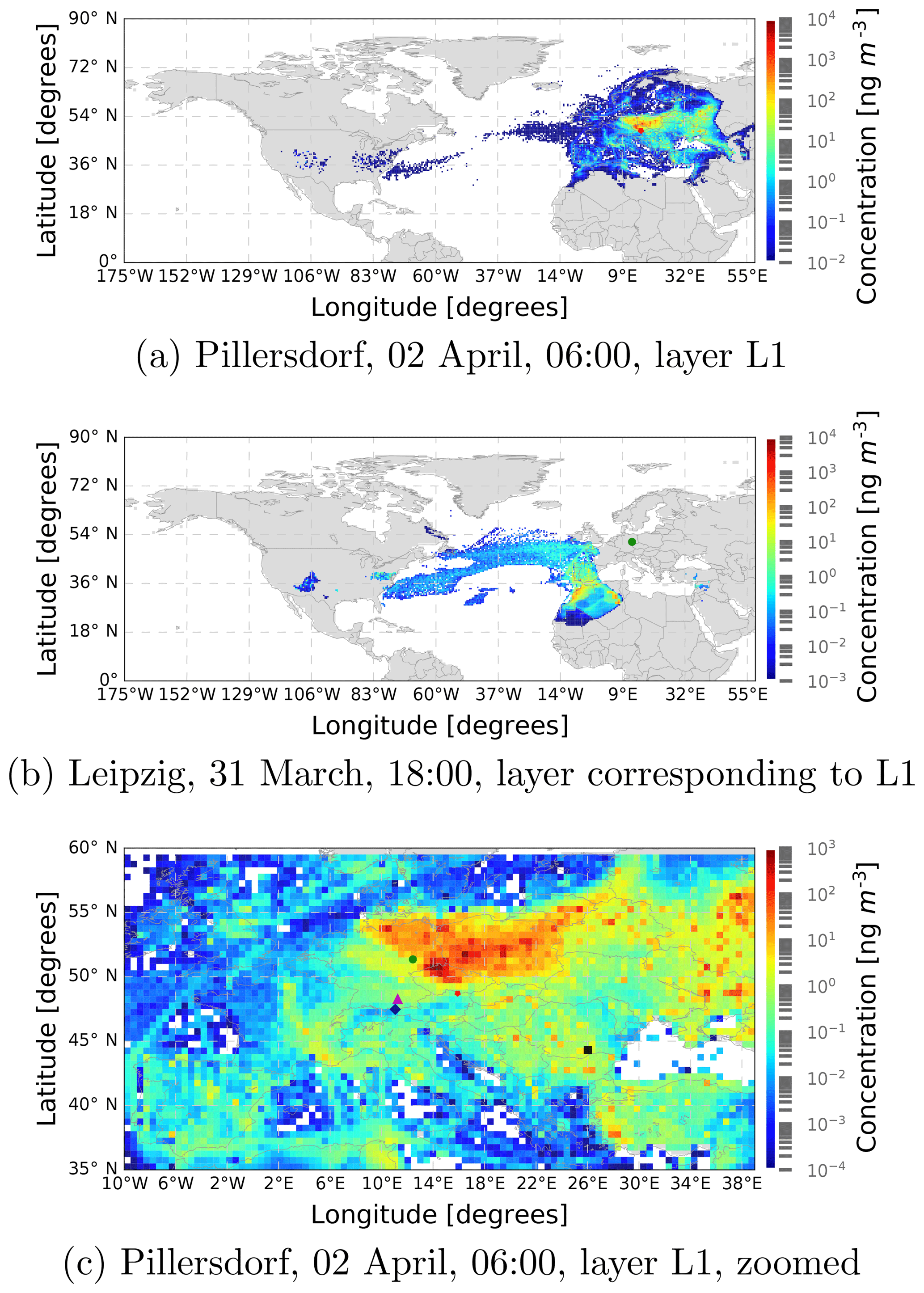
Figure 10 Relative distributions of SO₂ sources for Pillersdorf layer L1 (a), Leipzig (b); zoomed distribution for Pillersdorf layer L1 (c).

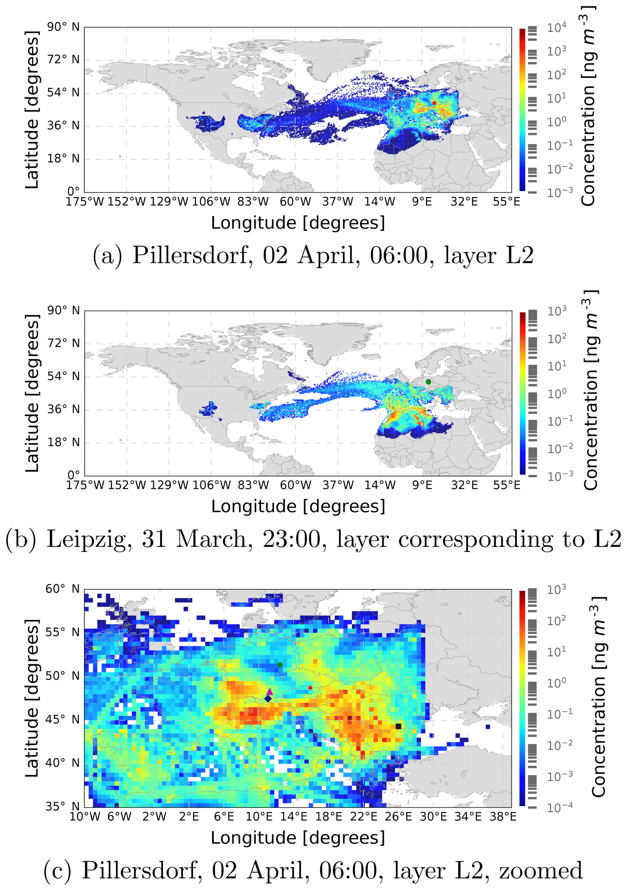
Figure 11 Relative distributions of SO₂ sources for Pillersdorf layer L2 (a), Leipzig (b); zoomed distribution for Pillersdorf layer L2 (c).

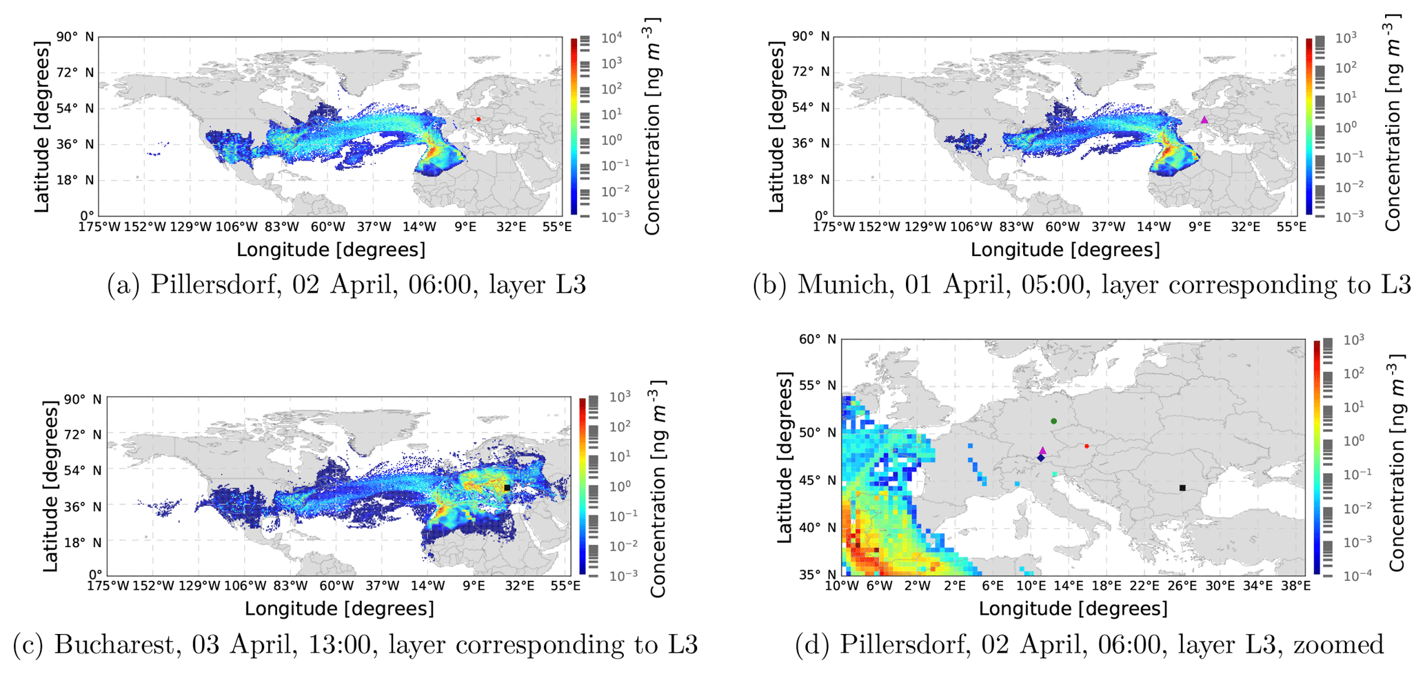
Figure 12 Relative distributions of SO₂ sources for Pillersdorf layer L3 (a), Munich (b), and Bucharest (c); zoomed distribution for Pillersdorf layer L3 (d).

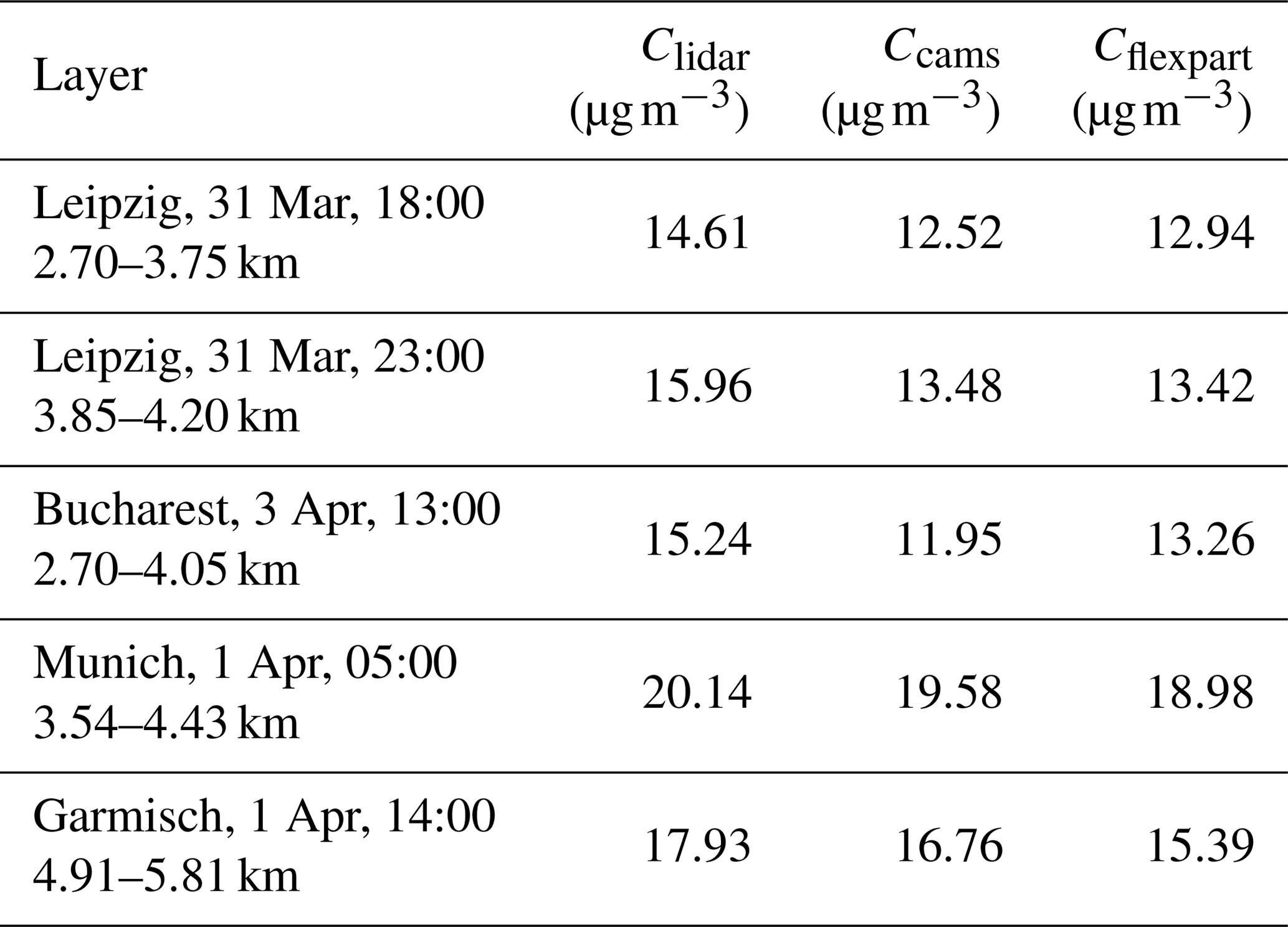
For the lidar stations, a comparison of concentrations computed from the lidar measurements with the sulfate concentrations computed from CAMS values for the lidar station location and the concentrations computed from the modeled SRS are given in Table 2.

Table 2 Comparison of sulfate concentration computed from lidar measurements, CAMS products, and FLEXPART for layers at lidar stations associated with layers from Pillersdorf, 2 April 2014, 06:00.

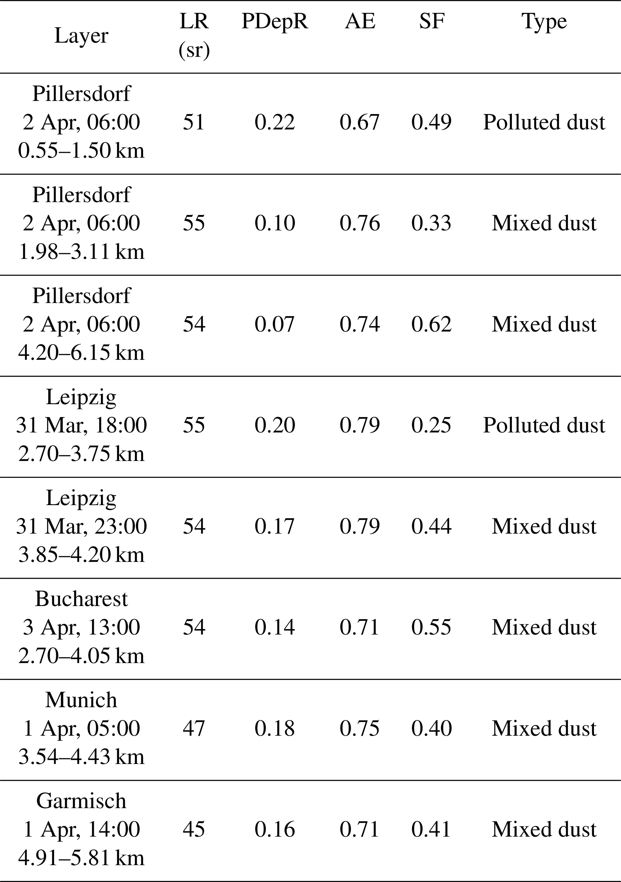
The optical properties, the sulfate fraction, and the aerosol types for the aerosol layers identified for Pillersdorf, 2 April, 06:00 and the associated layers at the lidar stations are given in Table 3. For Leipzig and Bucharest, the optical properties are computed from the lidar measurements; for Pillersdorf, Garmisch, and Munich they are computed using the NATALI model.

Table 3 Optical properties, sulfate fraction, and aerosol types for aerosol layers corresponding to Pillersdorf, 2 April 2014, 06:00.

The peak on 4 April was also analyzed similarly to the peak on 2 April. The corresponding vertical profiles of sulfate, dust, and total aerosol concentrations are shown in Fig. 13. From the backward- and forward-trajectory analyses, only one lidar station could be associated with a trajectory, for layer L2 at Pillersdorf at 12:00. The corresponding RCS at the lidar station is shown in Fig. 14. The SRS for the identified layers at Pillersdorf, 12:00, are presented in Fig. 15. Layers at Pillersdorf were associated with layers at the lidar stations; they are given in Table 4. The comparison of the aerosol concentrations at the overpassed lidar station is given in Table 5, and the optical properties are given in Table 6.

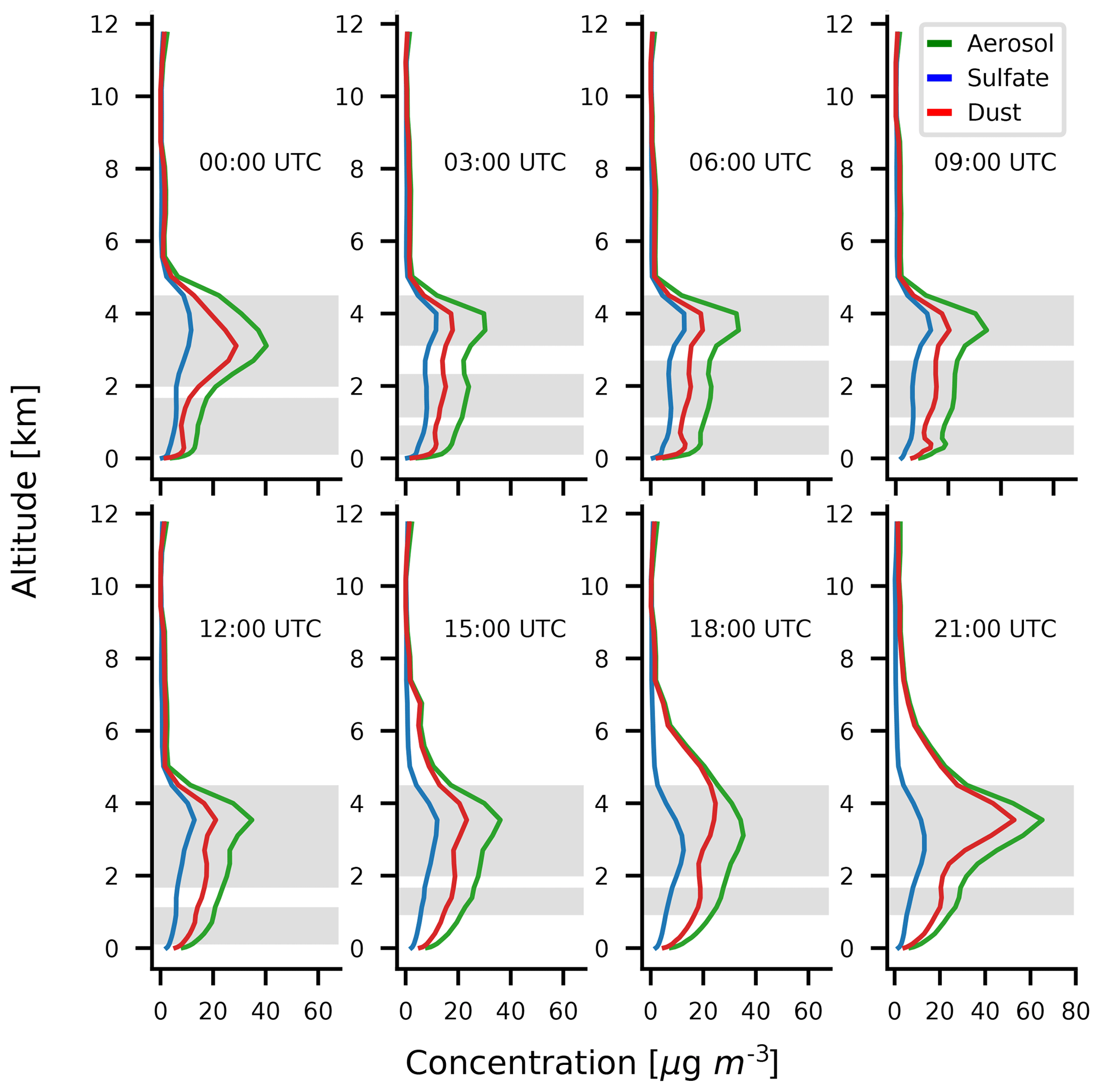
Figure 13 CAMS aerosol, sulfate, and dust profiles for 4 April 2014, Pillersdorf. The gray area represents the identified sulfate layers. Altitudes are given in kilometers above ground level.

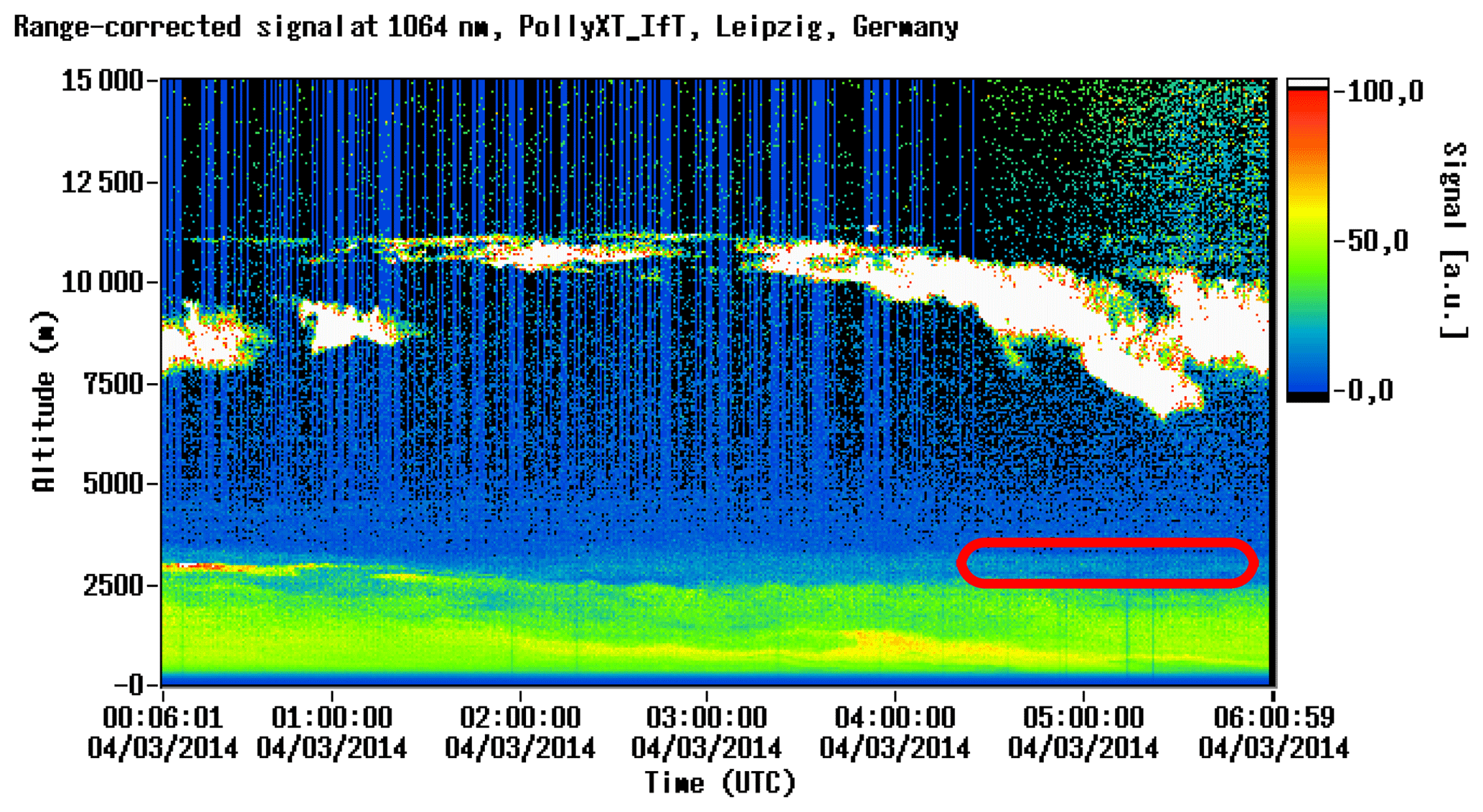
Figure 14 Range-corrected signal at 1064 nm for Leipzig station, 3 April 2014. The red box represents the identified layer.

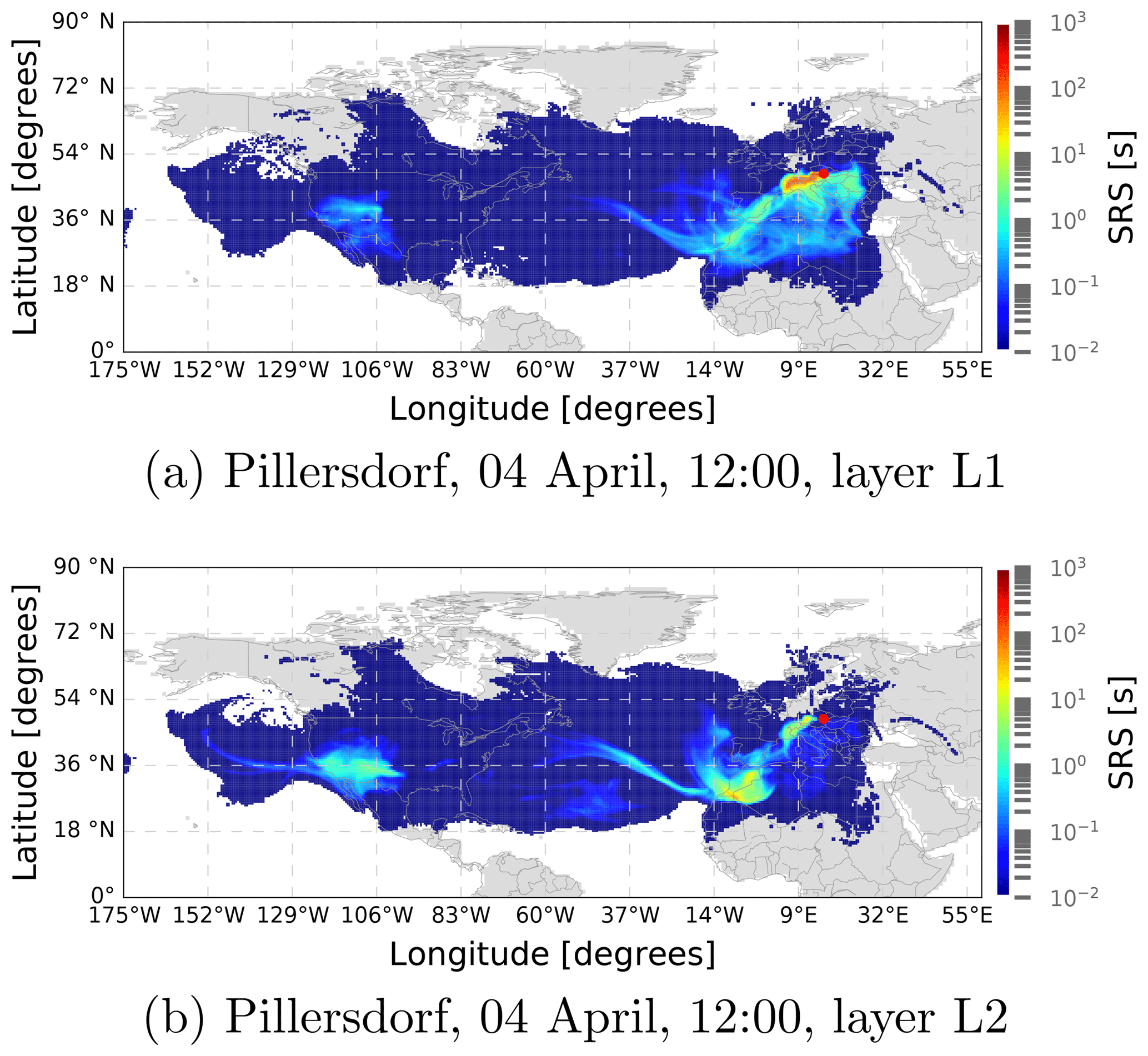
Figure 15 Source–receptor sensitivity for layers L1 (a) and L2 (b), Pillersdorf, 4 April, 12:00.

Table 4 Association of layers from lidar measurements with layers and trajectories computed for Pillersdorf, 4 April 2014, 12:00.

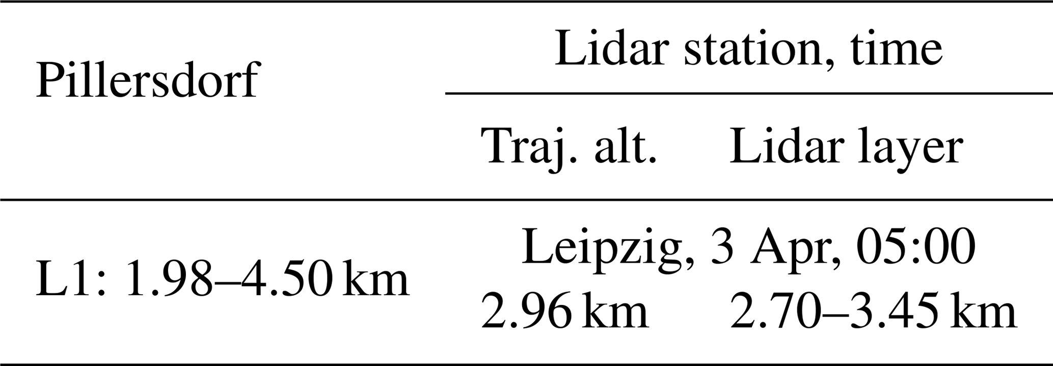
Table 5 Comparison of sulfate concentration computed from lidar measurements, CAMS data and FLEXPART for layers at lidar stations associated with layers from Pillersdorf, 4 April 2014, 12:00.

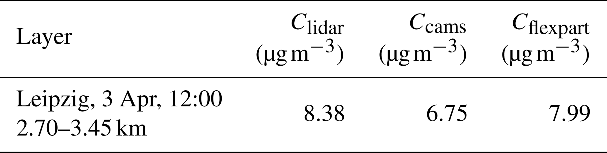
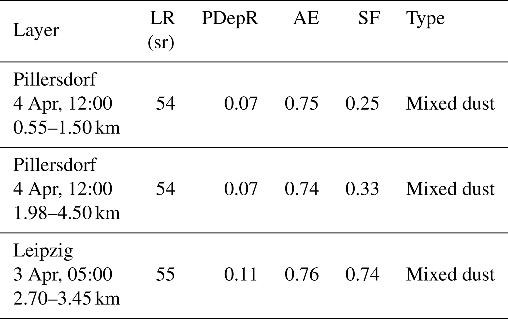
Table 6 Optical properties, sulfate fraction, and aerosol types for aerosol layers corresponding to Pillersdorf, 4 April 2014, 12:00.

3.2 Discussion of the results

The daily variations in the in situ measurements of SO₂, O₃, PM_2.5, and PM₁₀ concentrations depend on more factors, such as variations in source emissions, photochemical reactions, meteorological conditions, planetary boundary layer heights, and short-, medium-, and long-range transport of aerosols.

Figure 1 indicates a period between 27 March and 6 April in which in situ measurements of SO₂, O₃, PM_2.5, and PM₁₀ concentrations recorded at Pillersdorf exceed the averaged values for the period 15 March–14 April 2014. A significant load of aerosols in the atmosphere in this period is also confirmed by the AOD values between 0.07 and 0.73 for Pillersdorf, retrieved from CAMS products, which are above the AOD threshold of 0.06 for clear atmosphere (Kaskaoutis et al., 2012). For the period 27 to 31 March, no significant load of aerosols is observed at the lidar stations around Pillersdorf; therefore no medium- or long-range transport of aerosols is involved. The source–receptor sensitivity computed for 31 March (not shown) points to a short-range-transported event, of small duration and at low altitude, with sources in the southeast of Austria. This event is not described in this paper.

From a qualitative analysis of in situ concentrations for PM₁₀, PM_2.5, and SO₂ (Fig. 1) and the CAMS time series of mixing ratios for dust, sulfate, and total aerosol at Pillersdorf (Fig. 2) and the lidar stations around Pillersdorf (Fig. 3), the presence of an event of sulfate transport over Europe can be inferred, with two peaks, on 2 and 4 April.

On 2 April, one observes from the concentration profiles (Fig. 4) that in the morning the dust was dominant in the layer between 0.55 and 1.50 km and in the layer between 1.98 and 3.11 km, while sulfate was dominant in the higher-altitude layer, between 4.20 and 6.15 km. In the afternoon, the sulfate concentration increased gradually in the lower layers, mixing with the dust, while the upper layer became thinner (layer range from 4.0 to 5.0 km).

The back trajectories for 2 April (Fig. 5) show a consistent pattern. In the morning (00:00 and 06:00), the lower trajectories (below 2000 m) originate from the eastern and southern United States (US), traverse the North Atlantic Ocean, and pass over central Europe, spending ∼6 d in this region, arriving at Pillersdorf from the northwest direction. The middle-altitude trajectories (2000–5000 m) originate from the southern US, traverse the ocean, and pass over northwest Africa (spending ∼3 d in the region), arriving in the central Europe from the southwest, then arriving along the Alps at Pillersdorf. The high-altitude trajectories (above 5000 m) traverse the ocean, arriving at Pillersdorf from the west. In the afternoon (12:00 and 18:00), the lower trajectories originate from eastern Europe, while the middle-altitude and high-altitude trajectories originate from the eastern US, traverse the ocean and northwest Africa, and arriving at Pillersdorf from the west.

The SRS patterns, shown in Fig. 9, and the relative distributions of SO₂, shown in Figs. 10, 11, and 12, indicate the influence of five source regions for the transport of the sulfate event recorded on 2 April at Pillersdorf: the southern and eastern US, northwest Africa, central Europe, and eastern Europe.

For the lower layers, central Europe, including industrial centers from the “Black Triangle” (eastern Germany, southwest Poland, and Czech Republic), was the main source contributing to sulfate transported over northern Austria, where the Pillersdorf station is situated. Medium to smaller contributions come from sources in eastern Europe, northwest Africa, and the eastern US.

For the middle-altitude layers, sources from central Europe (northern Italy, Serbia, Hungary) contribute with similar emissions. Northwest Africa and the eastern US also have important contributions.

For the high-altitude layers, the main contributions come from northwest Africa, but sources from the southern and eastern US also contribute significantly. No contributions from Europe are seen for these layers.

For the peak on 4 April, having only one lidar station associated with aerosol trajectories, the analysis is more difficult. From the existing information, we can conclude that the pattern is similar to layers L2 and L3 from 2 April, with contributions from northern Italy, northwest Africa, and the southern US.

The AEs for the event have values between 0.67 and 0.79, which correspond to a mixture of fine and coarse particles, with size distribution centered on 0.75 µm. For this size distribution, the sulfate (Ding et al., 2017) and the dust (accumulation mode) are the dominant aerosols. The LR is comparable for all sites, having values between 45 and 55 sr, while the linear PDepR has values between 0.07 and 0.22. These values correspond to low- to medium-absorbing aerosol with a nonspherical shape (Nicolae et al., 2018).

The aerosol type is determined from the optical properties for the layers identified in this event, at the in situ station and the lidar stations. A consistent aerosol type was found between the in situ station and the lidar stations along the trajectories. The changes in the values of the aerosol LR, AE, and linear PDepR along the trajectories can be explained by

• the mixing of dust with secondary sulfate from anthropogenic sources during the transport paths to Leipzig, Munich, Garmisch-Partenkirchen, Pillersdorf, and Bucharest and

• the adsorption of the SO₂ on oxides contained in the mineral dust. The sulfate particles are expected to be formed by SO₂ oxidizing on dust surface due to mineral oxide compounds from dust (e.g., hematite).

4 Conclusions

The excess of SO₂, PM_2.5, PM₁₀, and O₃ observed in the period 1–6 April 2014 at the Austrian air quality background station Pillersdorf was analyzed using in situ data, lidar measurements at the closest EARLINET stations around the in situ site, CAMS near-real-time data, and aerosol and atmospheric transport modeling. This excess was associated with the transport of sulfate aerosols, mixed during the transport with dust. By correlating the local information with a trajectory analysis and an analysis of aerosol potential sources, a complex pattern of contributions to sulfate at the in situ station was found. The lower layers (below 2000 m) originated mainly from central Europe. Medium to smaller contributions came from sources in eastern Europe, northwest Africa, and the eastern US. For the middle-altitude layers (between 2000 and 5000 m), sources from central Europe (northern Italy, Serbia, Hungary) contributed with similar emissions. Northwest Africa and the eastern US also have important contributions. The high-altitude layers (above 5000 m) originated from sources from northwest Africa and from the southern and eastern US, as transported secondary sulfate mixed with dust. The effect of medium- and long-range transport of aerosol is significant, and can not be neglected when analyzing the air quality at an in situ station. For a quantitative analysis and modeling of aerosol deposition, more measurements are needed, including precise vertical aerosol profiles at the in situ station.

The spring period studied in this paper is characterized by low, if any, deep convection. For the summer period, one expects, however, to have strong convective activity over central Europe. A study of the summer periods for the years 2014–2017 for the same region was also performed; the results will be presented in a separate paper.

The methodology developed in this paper allows us to obtain a better understanding of the effects of aerosol transport on the in situ measurements. It can be used as a general tool to correlate measurements at in situ stations with ground-based remote-sensing stations located around these in situ stations. A dedicated paper for the methodology, extended to trace gases and other aerosols, with analysis of more case studies is under preparation.