the Creative Commons Attribution 4.0 License.
the Creative Commons Attribution 4.0 License.
 | 30 Apr 2019
Calibration of a multi-physics ensemble for estimating the uncertainty of a greenhouse gas atmospheric transport model
Liza I. Díaz-Isaac
Thomas Lauvaux
Marc Bocquet
Kenneth J. Davis
Atmospheric inversions have been used to assess biosphere–atmosphere CO2 surface exchanges at various scales, but variability among inverse flux estimates remains significant, especially at continental scales. Atmospheric transport errors are one of the main contributors to this variability. To characterize transport errors and their spatiotemporal structures, we present an objective method to generate a calibrated ensemble adjusted with meteorological measurements collected across a region, here the upper US Midwest in midsummer. Using multiple model configurations of the Weather Research and Forecasting (WRF) model, we show that a reduced number of simulations (less than 10 members) reproduces the transport error characteristics of a 45-member ensemble while minimizing the size of the ensemble. The large ensemble of 45 members was constructed using different physics parameterization (i.e., land surface models (LSMs), planetary boundary layer (PBL) schemes, cumulus parameterizations and microphysics parameterizations) and meteorological initial/boundary conditions. All the different models were coupled to CO2 fluxes and lateral boundary conditions from CarbonTracker to simulate CO2 mole fractions. Observed meteorological variables critical to inverse flux estimates, PBL wind speed, PBL wind direction and PBL height are used to calibrate our ensemble over the region. Two optimization techniques (i.e., simulated annealing and a genetic algorithm) are used for the selection of the optimal ensemble using the flatness of the rank histograms as the main criterion. We also choose model configurations that minimize the systematic errors (i.e., monthly biases) in the ensemble. We evaluate the impact of transport errors on atmospheric CO2 mole fraction to represent up to 40 % of the model–data mismatch (fraction of the total variance). We conclude that a carefully chosen subset of the physics ensemble can represent the uncertainties in the full ensemble, and that transport ensembles calibrated with relevant meteorological variables provide a promising path forward for improving the treatment of transport uncertainties in atmospheric inverse flux estimates.
- Article
(7924 KB) - Full-text XML
- BibTeX
- EndNote


Atmospheric inversions are used to assess the exchange of CO2 between the biosphere and the atmosphere (e.g., Gurney et al., 2002; Baker et al., 2006; Peylin et al., 2013). The atmospheric inversion or “top-down” method combines a prior distribution of surface fluxes with a transport model to simulate CO2 mole fractions and adjust the fluxes to be optimally consistent with the observations (Enting, 1993). Large uncertainty and variability often exist among inverse flux estimates (e.g., Gurney et al., 2002; Sarmiento et al., 2010; Peylin et al., 2013; Schuh et al., 2013). These posterior flux uncertainties arise from varying spatial resolution, limited atmospheric data density (Gurney et al., 2002), uncertain prior fluxes (Corbin et al., 2010; Gourdji et al., 2010; Huntzinger et al., 2012) and uncertainties in atmospheric transport (Stephens et al., 2007; Gerbig et al., 2008; Pickett-Heaps et al., 2011; Díaz Isaac et al., 2014; Lauvaux and Davis, 2014).
Atmospheric inversions based on Bayesian inference depend on the prior flux error covariance matrix and the observation error covariance matrix. The prior flux error covariance matrix represents the statistics of the mismatch between the true fluxes and the prior fluxes, but the limited density of flux observation limits our ability to characterize these errors (Hilton et al., 2013). The observation error covariance describes errors of both measurements and the atmospheric transport model. In atmospheric inversions, the model errors tend to be much greater than the measurement errors (e.g., Gerbig et al., 2003; Law et al., 2008). Additionally, atmospheric inversions assume that the atmospheric transport uncertainties are known and are unbiased; therefore, the method propagates uncertain and potentially biased atmospheric transport model errors to inverse fluxes limiting their optimality. Unfortunately, rigorous assessments of the transport uncertainties within current atmospheric inversions are limited. Estimation of the atmospheric transport errors and their impact on CO2 fluxes remains a challenge (Lauvaux et al., 2009).
A limited number of studies are dedicated to quantify the uncertainty in atmospheric transport models and even fewer attempted to translate this information into the impact on the CO2 mixing ratio and inverse fluxes. The atmospheric Tracer Transport Model Intercomparison Project (TransCom) has been dedicated to evaluate the impact of atmospheric transport models in atmospheric inversion systems (e.g., Gurney et al., 2002; Law et al., 2008; Peylin et al., 2013). These experiments have also shown the importance of the transport model resolution to avoid any misrepresentation of high-frequency atmospheric signals (Law et al., 2008). Diaz Isaac et al. (2014) showed how two transport models with two different resolutions and physics but using the same surface fluxes can lead to large model–data differences in the atmospheric CO2 mole fractions. These differences would yield significant errors on the inverse fluxes if propagated into the inverse problem. Errors in horizontal wind (Lin and Gerbig, 2005) and in vertical transport (Stephens et al., 2007; Gerbig et al., 2008; Kretschmer et al., 2012) have been shown to be important contributors to uncertainties in simulated atmospheric CO2. Lin and Gerbig (2005), for example, estimate the impact of horizontal wind error on CO2 mole fractions and conclude that uncertainties in CO2 due to advection errors can be as large as 6 ppm. Other studies have shown that errors in the simulation of vertical mixing have a large impact on simulated CO2 and inverse flux estimates (e.g., Denning et al., 1995; Stephens et al., 2007; Gerbig et al., 2008). Therefore, some studies have evaluated the effects that planetary boundary layer height (PBLH) has on CO2 mole fractions (Gerbig et al., 2008; Williams et al., 2011; Kretschmer et al., 2012). Approximately 3 ppm uncertainty in CO2 mole fractions has been attributed to PBLH errors over Europe during the summertime (Gerbig et al., 2008; Kretschmer et al., 2012). These studies have attributed the errors to the lack of sophisticated subgrid parameterization, especially PBL schemes and land surface models (LSMs). This led other studies (Kretschmer et al., 2012; Lauvaux and Davis, 2014; Feng et al., 2016) to evaluate the impact of different PBL parameterizations on simulated atmospheric CO2. These studies have found systematic errors of several ppm in atmospheric CO2 that can generate biased inverse flux estimates. While there is an agreement that errors in the vertical mixing and advection schemes can directly affect the inverse fluxes, other components of the model physics (e.g., convection, large-scale forcing) have not been carefully evaluated.
Atmospheric transport models have multiple sources of uncertainty including the boundary conditions, initial conditions, model physics parameterization schemes and parameter values. With errors inherited from all of these sources, ensembles have become a powerful tool for the quantification of atmospheric transport uncertainties. Different approaches have been evaluated in the carbon cycle community to represent the model uncertainty: (1) the multi-model ensembles that encompass models from different research institutions around the world (e.g., TransCom experiment; Gurney et al., 2002; Baker et al., 2006; Patra et al., 2008; Peylin et al., 2013; Houweling et al., 2010), (2) multi-physics ensembles that involve different model physics configurations generated by the variation of different parameterization schemes from the model (e.g., Kretschmer et al., 2012; Yver et al., 2013; Lauvaux and Davis, 2014; Angevine et al., 2014; Feng et al., 2016; Sarmiento et al., 2017) and (3) multi-analysis (i.e., forcing data) that consists of running a model over the same period using different analysis fields (where perturbations can be added) (e.g., Lauvaux et al., 2009; Miller et al., 2015; Angevine et al., 2014). These ensembles are informative (e.g., Peylin et al., 2013; Kretschmer et al., 2012; Lauvaux and Davis, 2014) but have some shortcomings. In some cases, the ensemble spread includes a mixture of transport model uncertainties and other errors such as the variation in prior fluxes or the observations used. Other studies have only varied the PBL scheme parameterizations. None of these studies have carefully assessed whether or not their ensemble spreads represent the actual transport uncertainties.
In the last two decades, the development of ensemble methods has improved the representation of transport uncertainty using the statistics of large ensembles to characterize the statistical spread of atmospheric forecasts (e.g., Evensen, 1994a, b). Single-physics ensemble-based statistics are highly susceptible to model error, leading to underdispersive ensembles (e.g., Lee, 2012). Large ensembles (> 50 members) remain computationally expensive and ill adapted to assimilation over longer timescales such as multi-year inversions of long-lived species (e.g., CO2). Smaller-size ensembles would be ideal, but most initial-condition-only perturbation methods produce unreliable and overconfident representations of the atmospheric state (Buizza et al., 2005). An ensemble used to explore and quantify atmospheric transport uncertainties requires a significant number of members to avoid sampling noise and the lack of dispersion of the ensemble members (Houtekamer and Mitchell, 2001). However, large ensembles are computationally expensive. Limitations in computational resources lead to restrictions, including the setup of the model (e.g., model resolution, nesting options, duration of the simulation) and the number of ensemble members. It is desirable to generate an ensemble that is capable of representing the transport uncertainties and which does not include any redundant members.
Various post-processing techniques can be used to calibrate or “down-select” from a transport ensemble of 50 or more members to a subset of ensemble members that represent the model transport uncertainties (e.g., Alhamed et al., 2002; Garaud and Mallet, 2011; Lee, 2012; Lee et al., 2016). Some of these techniques are principal component analysis (e.g., Lee, 2012), k-means cluster analysis (e.g., Lee et al., 2012) and hierarchical cluster analysis (e.g., Alhamed et al., 2002; Yussouf et al., 2004; Johnson et al., 2011; Lee et al., 2012, 2016). Riccio et al. (2012) applied the concept of “uncorrelation” to reduce the number of members without using any observations. Solazzo and Galmarini (2014) reduced the number of members by finding a subset of members that maximize a statistical performance skill such as the correlation coefficient, the root mean square error or the fractional bias. Other techniques applied less commonly to the calibration of the ensembles include simulated annealing and genetic algorithms (e.g., Garaud and Mallet, 2011). All these techniques are capable of eliminating those members that are redundant and generating an ensemble with a smaller number of members that represents the uncertainty of the atmospheric transport model more faithfully than the larger ensemble.
In this study, we start with a large multi-physics/multi-analysis ensemble of 45 members presented in Díaz-Isaac et al. (2018) and apply a calibration process similar to the one explained in Garaud and Mallet (2011). Two principal features characterize an ensemble: reliability and resolution. The reliability is the probability that a simulation has of matching the frequency of an observed event. The resolution is the ability of the system to predict a specific event. Both features are needed in order to represent model errors accurately. Our main goal is to down-select the large ensemble to generate a calibrated ensemble that will represent the uncertainty of the transport model with respect to meteorological variables of most importance in simulating atmospheric CO2. These variables are the horizontal mean PBL wind speed and wind direction, and the vertical mixing of surface fluxes, i.e., PBLH. We focus on the criterion that will measure the reliability of the ensemble, i.e., the probability of the ensemble in representing the frequency of events (i.e., the spatiotemporal variability of the atmospheric state). For the down-selection of the ensemble, we will use two different techniques: simulated annealing and a genetic algorithm (from now on referred to as calibration techniques/processes). In a final step, the ensemble with the optimal reliability will be selected by minimizing the biases in the ensemble mean. We will evaluate which physical parameterizations play important roles in balancing the ensembles and evaluate how well a pure physics ensemble can represent transport uncertainty.
2.1 Generation of the ensemble
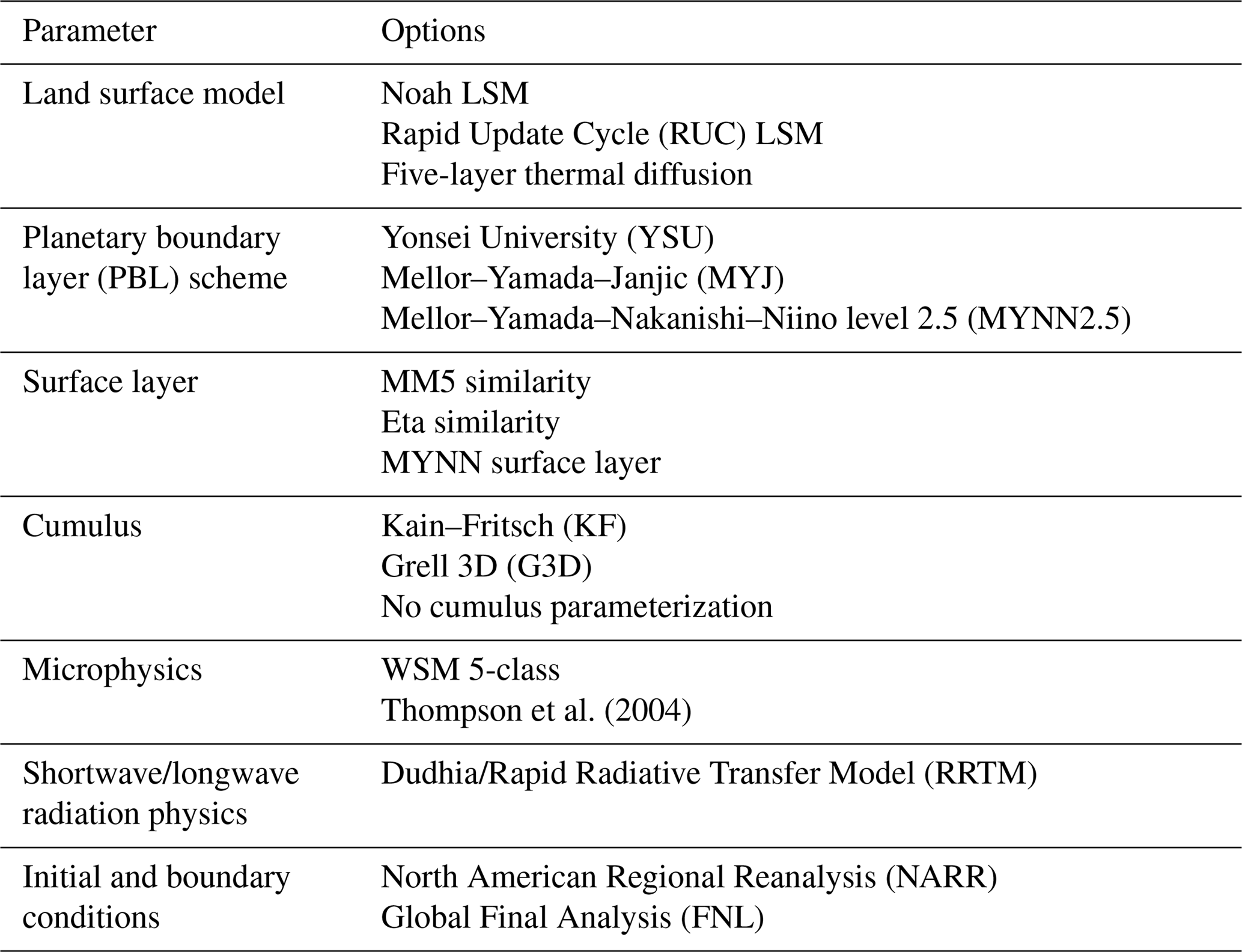
We generate an ensemble using the Weather Research and Forecasting (WRF) model version 3.5.1 (Skamarock et al., 2008), including the chemistry module modified in this study for CO2 (WRF-ChemCO2). The ensemble consists of 45 members that were generated by varying the different physics parameterization and meteorological data. The land surface models, surface layers, planetary boundary layer schemes, cumulus schemes, microphysics schemes and meteorological data (i.e., initial and boundary conditions) are alternated in the ensemble (see Table 1). All the simulations use the same radiation schemes, both long- and shortwave.
Table 1Physics schemes used in WRF for the sensitivity analysis.
The different simulations were run using the one-way nesting method, with two nested domains (Fig. 1). The coarse domain (d01) uses a horizontal grid spacing of 30 km and covers most of the United States and part of Canada. The inner domain (d02) uses a 10 km grid spacing, is centered in Iowa and covers the Midwest region of the United States. The vertical resolution of the model is described with 59 vertical levels, with 40 of them within the first 2 km of the atmosphere. This work focuses on the simulation with higher resolution; therefore, only the 10 km domain will be analyzed.
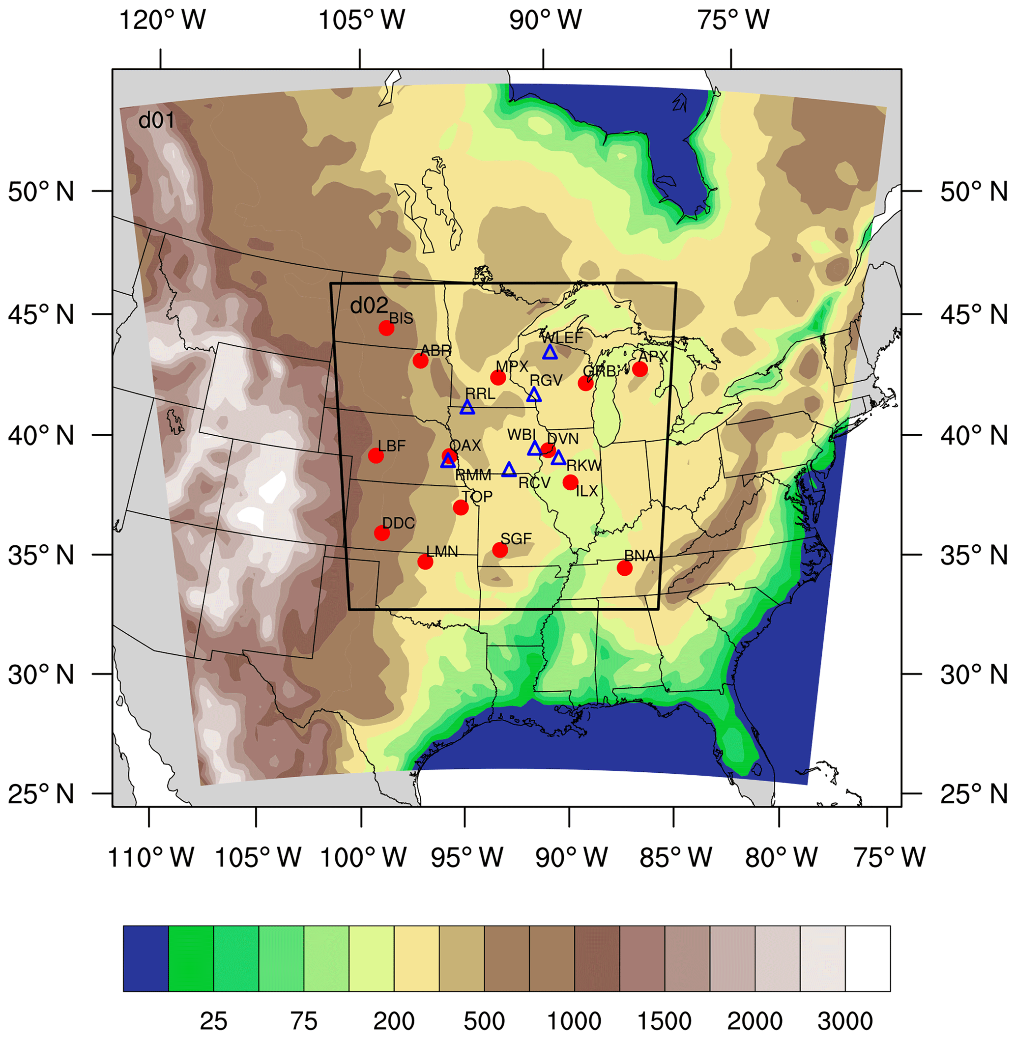
Figure 1Geographical domain used by WRF-ChemCO2 physics ensemble. The parent domain (d01) has a 30 km resolution, the inner domain (d02) has a 10 km resolution. Contours represent terrain height in meters. The inner domain covers the study region and includes the rawinsonde sites (red circles) and the CO2 towers (blue triangles) locations.
The CO2 fluxes for summer 2008 were obtained from NOAA Global Monitoring Division's CarbonTracker version 2009 (CT2009) data assimilation system (Peters et al., 2007; with updates documented at https://www.esrl.noaa.gov/gmd/ccgg/carbontracker/, last access: 17 January 2018). The different surface fluxes from CT2009 that we propagate into the WRF-ChemCO2 model are fossil fuel burning, terrestrial biosphere exchange and exchange with oceans. The CO2 lateral boundary conditions were obtained from CT2009 mole fractions. The CO2 fluxes and boundary conditions are identical for all ensemble members.
2.2 Dataset and data selection
Our interest is to calibrate the ensemble over the US Midwest using the meteorological observations available over this region. The calibration of the ensemble will be done only within the inner domain. To perform the calibration, we used balloon soundings collected over the Midwest region (Fig. 1). Meteorological data were obtained from the University of Wyoming's online data archive (http://weather.uwyo.edu/upperair/sounding.html, last access: 20 July 2018) for 14 rawinsonde stations over the US Midwest region (Fig. 1). To evaluate how the new calibrated ensemble impacts CO2 mole fractions, we will use in situ atmospheric CO2 mole fraction data provided by seven communication towers (Fig. 1). Five of these towers were part of a Penn State experimental network, deployed from 2007 to 2009 (Richardson et al., 2012; Miles et al., 2012, 2013; https://doi.org/10.3334/ORNLDAAC/1202). The other two towers (Park Falls – WLEF; West Branch – WBI) are part of the Earth System Research Laboratory/Global Monitoring Division (ESRL/GMD) tall tower network (Andrews et al., 2014), managed by NOAA. Each of these towers sampled air at multiple heights, ranging from 11 to 396 m above ground level (m a.g.l.).
The ensemble will be calibrated for three different meteorological variables: PBL wind speed, PBL wind direction and planetary boundary layer height (PBLH). We will calibrate the ensemble with the late afternoon data (i.e., 00:00 UTC) from the different rawinsondes. In this study, we use only daytime data, because we want to calibrate and evaluate the ensemble under the same well-mixed conditions that are used to perform atmospheric inversions. For each rawinsonde site, we will use wind speed and wind direction observations from approximately 300 m a.g.l. We choose this observational level because we want the observations to lie within the well-mixed layer, the layer into which surface fluxes are distributed, and the same air mass that is sampled and simulated for inversions based on tower CO2 measurements.
The PBLH was estimated using the virtual potential temperature gradient (θν). The method identifies the PBLH as the first point above the atmospheric surface layer, where (1) θν is greater than or equal to 0.2 K km−1, and (2) the difference between the surface and the threshold-level virtual potential temperature is greater than or equal to 3 K ( K).
WRF derives an estimated PBLH for each simulation; however, the technique used to estimate the PBLH varies according to the PBL scheme used to run the simulation. For example, the YSU PBL schemes estimate PBLH using the bulk Richardson number (Hong et al., 2006), the MYJ PBL scheme uses the turbulent kinetic energy (TKE) to estimate the PBLH (Janjic, 2002), and the MYNN PBL scheme uses twice the TKE to estimate the PBLH. To avoid any errors from the technique used to estimate the PBLH, we decided to estimate the PBLH from the model using the same method used for the observations. Simulated PBLH will be analyzed at the same time as the observations, 00:00 UTC, i.e., late afternoon in the study region.
We analyzed CO2 mole fractions collected from the sampling levels at or above 100 m a.g.l., which is the highest observation level across the Mid-Continent Intensive (MCI) network (Miles et al., 2012). This ensures that the observed mole fractions reflect regional CO2 fluxes and not near-surface gradients of CO2 in the atmospheric surface layer (ASL) or local CO2 fluxes (Wang et al., 2007). Both observed and simulated CO2 mole fractions are averaged from 18:00 to 22:00 UTC (12:00–16:00 LST), when the daytime period of the boundary layer should be convective and the CO2 profile well mixed (e.g., Davis et al., 2003; Stull, 1988). This averaged mole fraction will be referred to hereafter as daily daytime average (DDA).
2.3 Criteria
In this research, we want to test the performance of the transport ensemble and try to achieve a better representation of transport uncertainties, if possible using an ensemble with a smaller number of members. A series of statistical metrics are used as criteria to measure the representation of uncertainty by the ensemble for the period of 18 June to 21 July 2008. The criteria used for our down-selection process include rank histograms, rank-histogram scores and ensemble bias.
2.3.1 Talagrand diagram (or rank histogram) and rank-histogram score
The rank histogram and the rank-histogram scores are tools used to measure the spread and hence the reliability of the ensemble (see Fig. A1 in the Appendix). The rank histogram (Anderson, 1996; Hamill and Colucci, 1997; Talagrand et al., 1999) is computed by sorting the corresponding modeled variable of the ensemble in increasing order and then a rank among the sorted predicted variables from lowest to highest is given to the observation. The ensemble members are sorted to define “bins” of the modeled variable; if the ensemble contains N members, then there will be N+1 bins. If the rank is zero, then the observed variable value is lower than all the modeled variable values, and if it is N+1, then the observation is greater than all of the modeled values. If the ensemble is perfectly reliable, the rank histogram should be flat (i.e., flatness equal to 1). This happens when the probability of occurrence of the observation within each bin is equal. A rank histogram that deviates from the flat shape implies a biased, overdispersive or underdispersive ensemble. A “U-shaped” rank histogram indicates that the ensemble is underdispersive; normally, in this type of ensemble, the observations tend to fall outside of the envelope of the ensemble. This kind of histogram is associated with a lack of variability or an ensemble affected by biases (Hamill, 2001). A “central-dome” (or “A-shaped”) histogram indicates that the ensemble is overdispersive; this kind of ensemble has an excess of variability. If the rank histogram is overpopulated at either of the ends of the diagram, then this indicates that the ensemble is biased.
The rank-histogram score is used to measure the deviation from flatness of a rank histogram:
and should ideally be close to 1 (Talagrand et al., 1999; Candille and Talagrand, 2005). In Eq. (1), N is the number of members (i.e., models), M is the number of observations, rj the number of observations of rank j, and is the expectation of rj. In theory, the optimal ensemble has a score of 1 when enough members are available. A score lower than 1 would indicate overconfidence in the results, with an ensemble matching the observed variability better than statistically expected. Having a score smaller than 1 would not affect the selection process. Nevertheless, a flat rank histogram does not necessarily mean that the ensemble is reliable or has enough spread. For example, a flat histogram can still be generated from ensembles with different conditional biases (Hamill, 2001). The flat rank histogram can also be produced when covariances between samples are incorrectly represented. Therefore, additional verification analysis has to be introduced to certify that the calibrated ensemble has enough spread and is reliable. We introduce hereafter several additional metrics used to evaluate the ensemble.
2.3.2 Ensemble bias
Atmospheric inverse flux estimates are highly sensitive to biases. The bias, or the mean of the model–data mismatches, was used to assist the selection of the calibrated sub-ensemble. We identify a sub-ensemble that has minimal bias:
where pi is the difference between the modeled wind speed, direction or PBLH, and the observed value, M is the number of measurements and i sums over each of the rawinsonde measurements.
2.4 Verification methods
Different statistical tools were used to evaluate both the large (45-member) ensemble and calibrated ensemble; these statistics include Taylor diagrams, spread–skill relationship and ensemble root mean square deviation (RMSD). These statistical analyses will be used to describe the performance of each member (standard deviations and correlations), ensemble spread (root mean square deviation) and error structures in space (error covariance), which will allow us to evaluate all the important aspects of an ensemble.
We use Taylor diagrams to describe the performance of each of the models of the large ensemble (Taylor, 2001). The Taylor diagram relies on three nondimensional statistics: the ratio of the variance (model variance normalized by the observed variance), the correlation coefficient, and the normalized center root mean square (CRMS) difference (Taylor, 2001). The ratio of the variance or normalized standard deviation indicates the difference in amplitude between the model and the observation. The correlation coefficient measures the similarity in the temporal variation between the model and the observation. The CRMS is normalized by the observed standard deviation and quantifies the ratio of the amplitude of the variations between the model and the observations.
To verify that the ensemble captures the variability in the model performance across space and time, we computed the relationship between the spread of the ensemble and the skill of the ensemble over the entire dataset (i.e., spread–skill relationship). The linear fit between the two parameters measures the correlation between the ensemble spread and the ensemble mean error or skill (Whitaker and Lough, 1998). The ensemble spread is calculated by computing the standard deviation of the ensemble and the mean error by computing the absolute difference between the ensemble mean and the observations. Ideally, as the ensemble skill improves (the mean error gets smaller), the ensemble spread becomes smaller, and vice versa. Compared to the rank histograms, spread–skill diagrams represent the ability of the ensemble to represent the errors in time and space.
The spread of the ensemble is evaluated in time, using the RMSD. The RMSD does not consider the observations as we take the square root of the average difference between model configuration and the ensemble mean. Additionally, we use the mean and standard deviation of the error (model–data mismatch) to evaluate the performance of each of the members selected for the calibrated ensembles.
Transport model errors in atmospheric inversions are described in the observation error covariance matrix and hence in CO2 mole fractions (ppm2). Therefore, we evaluate the impact of the calibration on the variances of CO2 mole fractions. For the covariances, we compare the spatial extent of error structures between the full ensemble and the reduced-size ensembles by looking at spatial covariances from our measurement locations. The limited number of members is likely to introduce sampling noise in the diagnosed error covariances. We also know that the full ensemble is not a perfect reference, but we believe it is less noisy. The covariances were directly derived from the different ensembles to estimate the increase in sampling noise as a function of the ensemble size.
2.5 Calibration methods
In this study, we want to test the ability to reduce the ensemble from 45 members to an ensemble with a smaller number of members that is still capable of representing the transport uncertainties and does not include members with redundant information. The number of ideal ensemble members could have been decided by performing the calibration for all the different sizes of ensemble smaller than 45 members. However, we decided to use an objective approach to select the total number of members of the sub-ensemble. Therefore, we use the Garaud and Mallet (2011) technique to define the size of the calibrated sub-ensemble that each optimization technique will generate. The size of the sub-ensemble was determined by dividing the total number of observations by the maximum frequency in the large ensemble (45-member) rank histogram. We are going to generate sub-ensembles of three different sizes (number of members) to evaluate the impact that an ensemble size has on the representation of atmospheric transport uncertainties. Each of the ensembles will be calibrated for the period of 18 June to 21 July 2008.
Two optimization methods, simulated annealing (SA) and a genetic algorithm (GA), are used to select a sub-ensemble that minimizes the rank-histogram score (δ), which is the criterion that each algorithm will use to test the reliability of the ensemble. Each method will select a sub-ensemble that best represents the model uncertainties of PBL wind speed, PBL wind direction and PBLH.
In this study, SA and GA techniques will randomly search for the different combinations of members and compute the rank-histogram score. Both techniques generate a sub-ensemble (S) of size N. For the first test, we will use these algorithms to choose the combination of members that optimize the score of the reduced ensemble δ (S) (i.e., rank-histogram score) for each variable. With this evaluation, we determine if each optimization technique yields similar calibrated ensembles and if the calibrated ensembles are similar among the different meteorological variables. In the second test, we calibrate the ensemble for all three variables simultaneously, where we use the sum of the score squared: [δ(S)]2:
to control acceptance of the sub-ensembles. In Eq. (3), δwspd(S), δwdir(S) and δpblh(S) are the scores of the sub-ensemble for PBL wind speed, PBL wind direction and PBLH, respectively.
2.5.1 Simulated annealing
SA is a general probabilistic local search algorithm, described by Kirkpatrick et al. (1983) and Černý et al. (1985) as an optimization method inspired by the process of annealing in metal work. Based on the Monte Carlo iteration solving method, SA finds the global minimum using a cost function that gives to the algorithm the ability to jump or pass multiple local minima (see Fig. A2 in the Appendix). In this case, the optimal solution is a sub-ensemble with a rank-histogram score close to 1.
The SA starts with a randomly selected sub-ensemble. The current state (i.e., initial random sub-ensemble) has a lot of neighbor states (i.e., other randomly generated sub-ensembles) in which a unit (i.e., model) is changed, removed or replaced. Let S be the current sub-ensemble and S′ be the neighbor sub-ensemble. S′ is a new sub-ensemble (i.e., neighbor) that is randomly built from the current sub-ensemble with one model added, removed or replaced. To minimize the score δ, only two transitions to the neighbors are possible. In the first transition, if the score of the neighbor sub-ensembles δ(S′) is lower than the current sub-ensemble δ(S), then S′ becomes the current sub-ensemble and a new neighbor sub-ensemble is generated. In the second transition, if the score of the neighbor sub-ensemble δ(S′) is greater than the current sub-ensemble δ(S), moving to the neighbor S′ only occurs through an acceptance probability. This acceptance probability is equal to and it only allows the movement to the neighbor S′ if . For the acceptance probability, u is a random number uniformly drawn from [0,1] and T is called temperature, and it decreases after each iteration following a prescribed schedule. The acceptance probability is high at the beginning, and the probability of switching to a neighbor is less at the end of the algorithm. The possibility to select a less optimal state S′, i.e., with higher δ(S′), is meant to escape local minima where the algorithm could remain trapped.
When the algorithm reaches the predefined number of iterations, we collect only the accepted sub-ensemble S and their respective scores δ(S). When the algorithm finishes with the iterations, we choose the ensemble that has both the smallest rank-histogram score and lowest bias among the different sub-ensembles (see Sect. 2.7). The number of iterations was defined by sensitivity test and repetitivity of the experiments (see Sect. 2.6).
2.5.2 Genetic algorithm
GA is a stochastic optimization method that mimics the process of biological evolution, with the selection, crossover and mutation of a population (Fraser and Burnell, 1970; Crosby, 1973; Holland, 1975). Let Si be an individual, that is, a sub-ensemble, and let be a population of Npop individuals (see Fig. A3 in the Appendix). As a first step, in the GA, a random population is generated (denoted P0). Then this population will go through two out of the three steps of the genetic algorithm, (1) selection and (2) crossover. In the selection step, we select half of the best individuals with respect to the score (i.e., summation of the score of three variables δ(S)). For the second step, a crossover among the selected individuals occurs when two parents create two new children by exchanging some ensemble members. A new population is generated with Npop∕2 parents and Npop∕2 children.
This process is repeated until it reaches the specified number of iterations. This algorithm will provide at the end a population of individuals with a better rank-histogram score than the initial population. Out of all those individuals, we choose the sub-ensemble with the best score for the three variables (i.e., wind speed, wind direction and PBLH) and with a smaller bias than the large ensemble.
2.6 Parameterization of the selection algorithms
Various inputs are required to guide the selection algorithms. For example, we typically need to choose the initial and final temperature (T0 and Tf) for the SA and its schedule, the best population size (Npop) for the GA and the number of iterations for each algorithm. The temperature of the SA, the Npop of the GA and the number of iterations were chosen by running the algorithms multiple times and confirming that the system reached similar solutions with independent minimization runs. If similar solutions were not achieved within multiple SA or GA runs, the algorithm parameters were altered to increase the breadth of the search. For the SA, we found that 20 000 iterations yielded similar solutions after multiple runs of the algorithm. For the GA, 30 to 50 iterations were sufficient as long as the ensemble was smaller than eight members. For an ensemble of 10 members, we needed to increase to 100 iterations. Another factor that was important in the SA was the initial temperature used in the algorithm and the temperature decrease for each iteration. While the temperature is high, the algorithm will accept with more frequency the poorer solutions; as the temperature is reduced, the acceptance of poorer solutions is reduced. Therefore, we needed to provide an initial (T0) and final (Tf) temperature that allowed the system to reduce its acceptance condition gradually and to search more combinations of members to identify the best solution or sub-ensemble. We determine the optimal parameters for SA by the maximum number of ensemble solutions which indicates that the algorithm explored the largest space of solution with T0 equal to 20 and Tf equal to . For GA, the larger the population, the more we can explore the space to find an optimal solution. We found that a Npop of 280 individuals was the value that produced similar solutions (sub-ensembles) after multiple runs.
2.7 Selection of the optimal reduced-size ensembles
The selection process is performed in three distinct steps to ensure that the final calibrated ensembles will be the optimal combinations of model configurations (Fig. 2). First, the flatness of the rank histograms will control the acceptance of the calibrated sub-ensembles by the selection algorithms (see Fig. A1 in the Appendix). The flatness is defined by Eq. (1) for the single-variable calibration and Eq. (3) for the calibration of the three variables simultaneously. The algorithm selects multiple sub-ensembles with a rank-histogram score smaller than 6 for each individual meteorological variable, or smaller than the original ensemble score if higher than 6 (see Fig. 2 and Table 2). In general, the lowest scores are found for PBLH and the highest for wind speed, as shown in Fig. 3. As a second step, sub-ensembles accepted by SA and GA algorithms with a bias larger than the bias of the full ensemble are filtered out. This step is critical to avoid the selection of biased ensembles as discussed by Hamill et al. (2001). Finally, the remaining calibrated ensembles are compared among SA and GA techniques to identify if both algorithms provide a common solution. If multiple common solutions were identified, the final sub-ensemble was determined by the solution with the smallest score and bias. However, if no common solution was found by both techniques, the final sub-ensemble corresponds to the smallest score among the different solutions that share > 50 % of the same model configurations.
Table 2Rank-histogram score (δ), biases and standard deviation (σ) of the 45-member ensemble for wind speed, wind direction and PBLH computed across 14 rawinsonde sites using daily 00:00 UTC observations for 18 June to 21 July 2008 in the upper US Midwest.
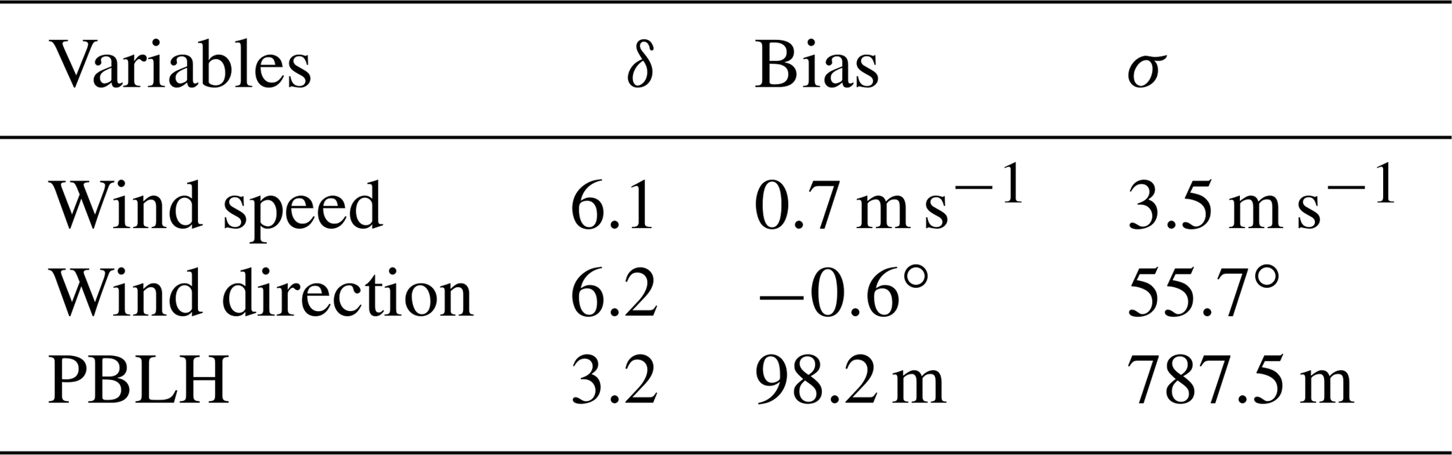
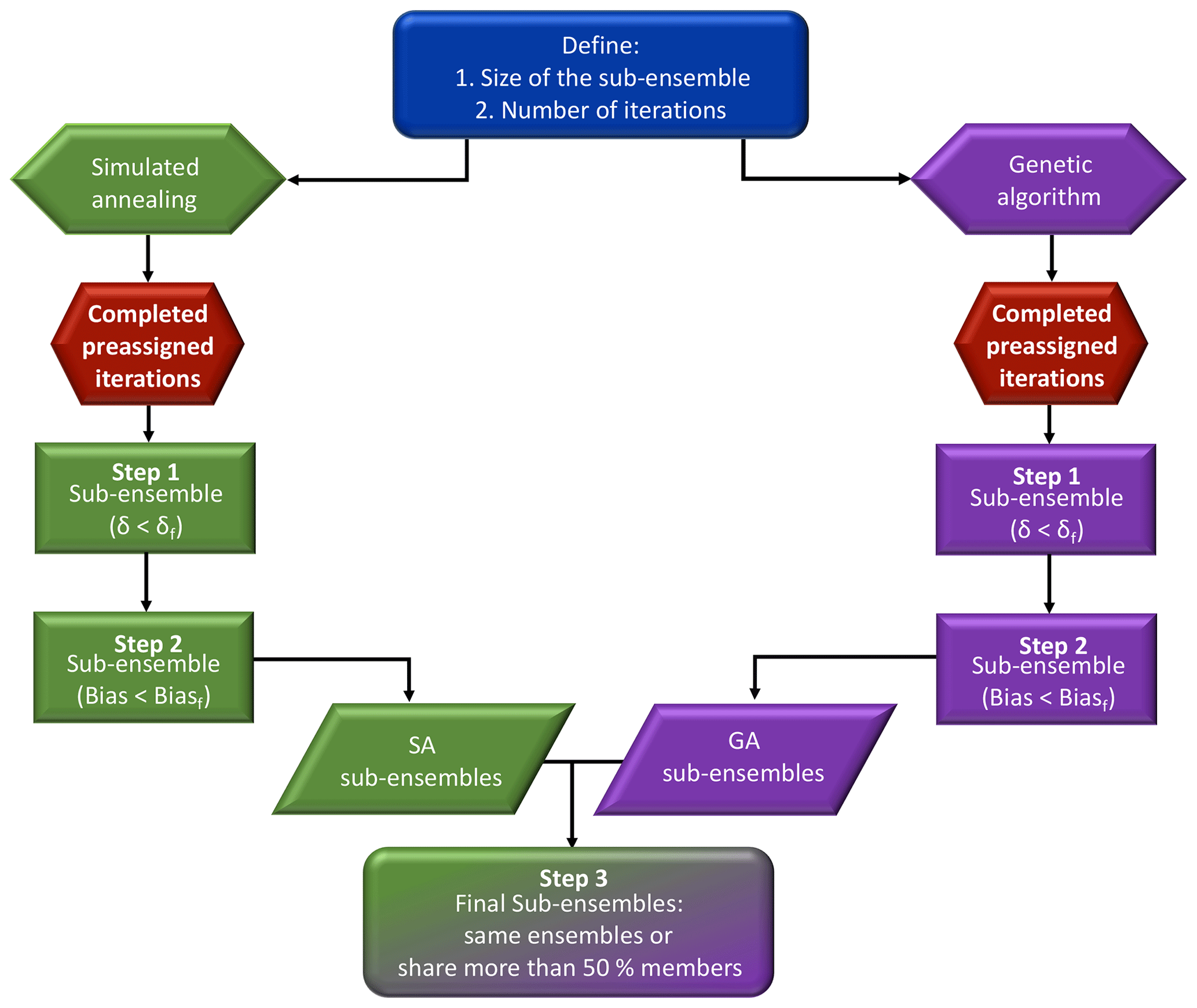
Figure 2Diagram of the process of selection of reduced-sized ensembles explained in Sect. 2.7. In this diagram, in the sub-ensemble, we show our two main thresholds after running each algorithm; the sub-ensemble score has to be smaller than the full ensemble (δ<δf) and the sub-ensemble bias is smaller than the full-ensemble bias (bias < biasf).

Figure 3Box plot of the rank-histogram scores of the different sub-ensembles of 10 (a), 8 (b) and 5 (c) members accepted by the SA. Each figure shows the rank-histograms scores for the different variables: PBL wind speed (WSPD), PBL wind direction (WDIR) and PBLH. The top of the box represents the 25th percentile, the bottom of the box is the 75th percentile, the red line in the middle is the median and the green “x” the mean. Outliers beyond the threshold values are plotted using the “+” symbol.
3.1 Evaluation of the large ensemble
In this section, we evaluate the performance of the large ensemble. Our goal is to test the ensemble skill (ability of the models to match the observations) and the spread (variability across model simulations to represent the uncertainty). We will evaluate the skill and the spread for PBLH, PBL wind speed and PBL wind direction across the region of study using afternoon (00:00 UTC) rawinsonde observations.
3.1.1 Model skill
We evaluate the performance of the different models of the 45-member ensemble by computing the normalized standard deviation, normalized center root mean square and correlation coefficient for wind speed (Fig. 4a), wind direction (Fig. 4b) and PBLH (Fig. 4c) (Taylor, 2001). The majority of the model configurations produce winds speeds and directions with higher standard deviations (more variability) than the observations, whereas the simulations over- and underestimate PBLH variability depending on the model configuration. The model–data correlations with wind speed and wind direction are between 0.4 and 0.7, whereas the PBLH shows a smaller correlation, between 0.3 and 0.6. The range of modeled PBL heights will provide a wide spectrum of alternatives to select the optimal calibrated sub-ensemble. However, wind speed and wind direction do not show much difference among the different models. This limited spread potentially reduces the selection of the model configurations to produce a sub-ensemble that matches the observed variability.
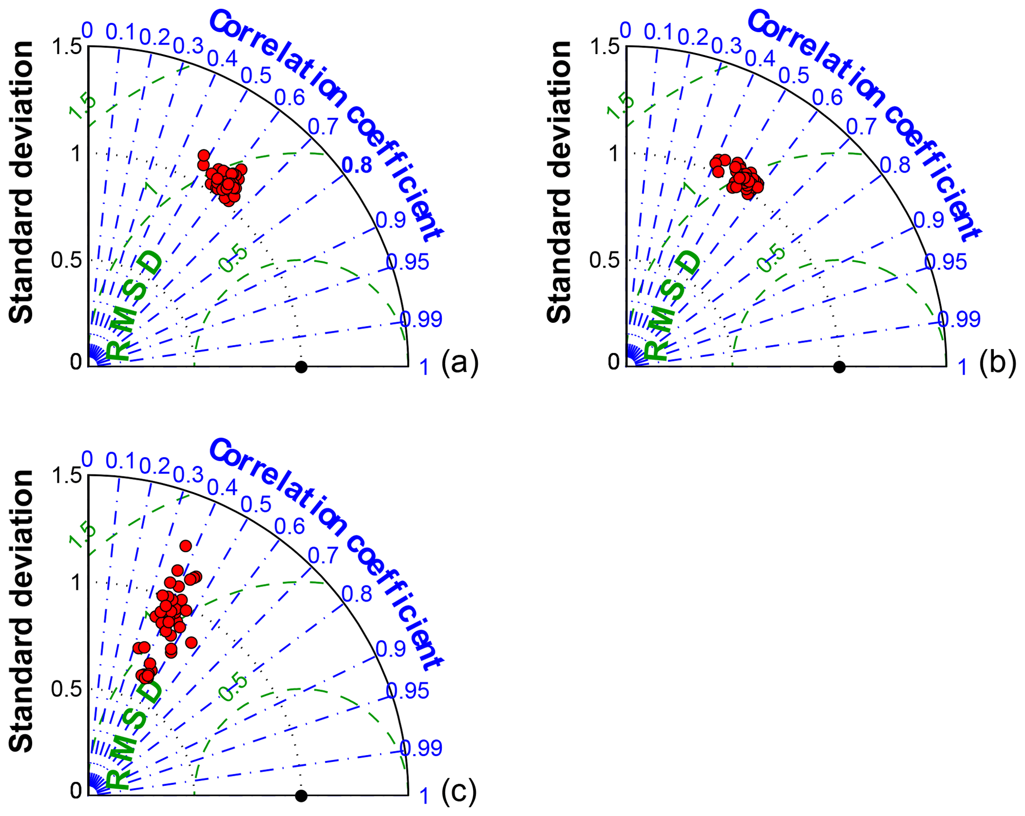
Figure 4Taylor diagram comparing the 00:00 UTC rawinsonde observations (300 m wind speed a, 300 m wind direction b and PBLH c) to the 45 model configurations (red circles).
3.1.2 Reliability and spread of the ensemble
We illustrate the ensemble spread and how well this ensemble encompasses the observations using the time series of the simulated and observed meteorological variables. Figure 5 shows the time series of the ensemble spread for wind speed, wind direction and PBLH at Green Bay (GRB; Fig. 5a, c, e) and Topeka (TOP; Fig. 5b, d, f) sites. The time series show qualitatively that simulated wind speed (Fig. 5a–b) and wind direction (Fig. 5c–d) have a smaller spread compared to PBLH (Fig. 5e–f). Figure 5 shows how the ensemble can have a small spread and still encompass the observations (i.e., DOY 183; Fig. 5c), and have a large spread and not encompass the observation (i.e., DOY 174; Fig. 5e). These time series suggest that the ensemble may struggle to encompass the observed wind speed and wind direction more than the PBLH.
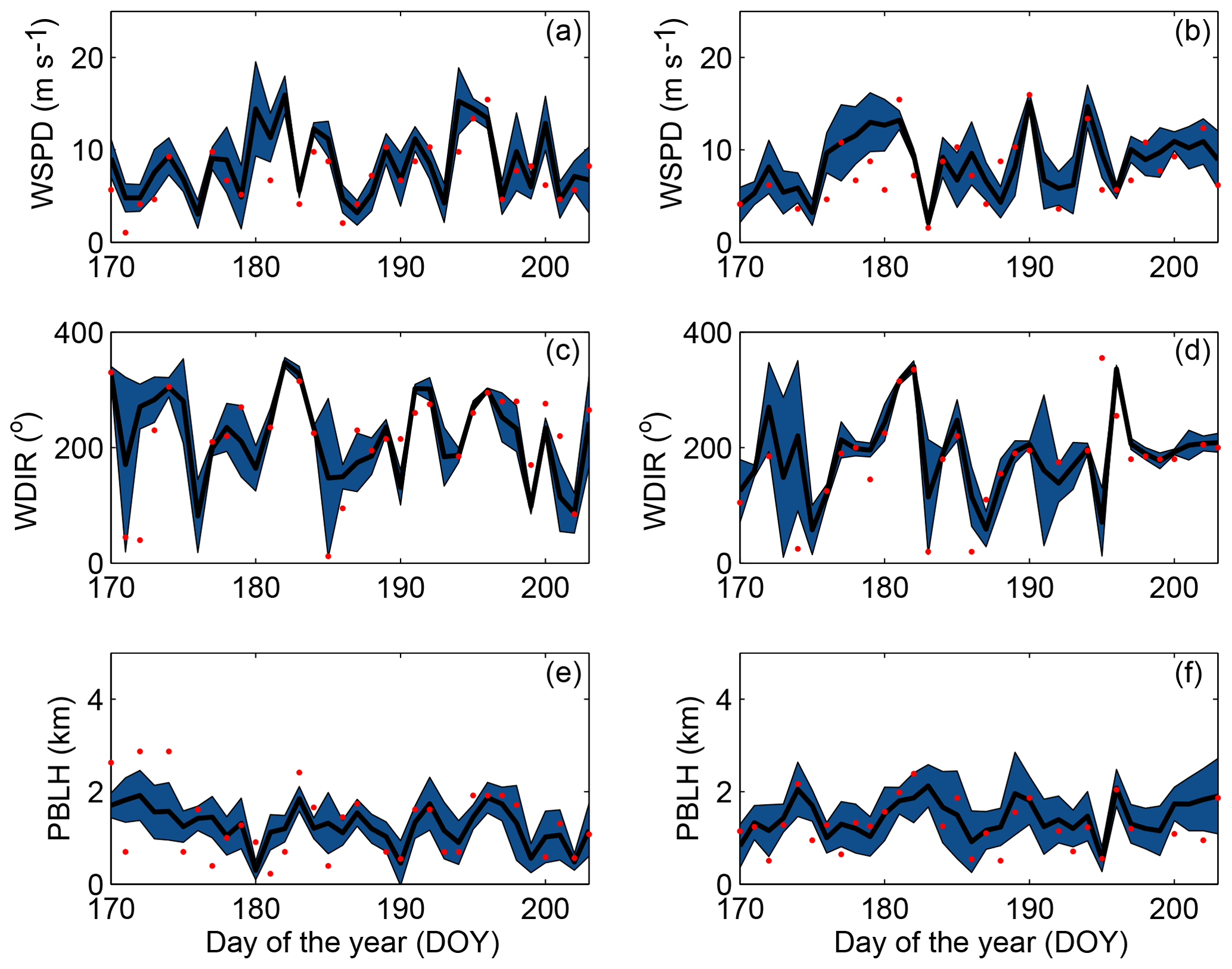
Figure 5Time series of the simulated and observed for 300 m wind speed (a, b), 300 m wind direction (c, d) and PBLH (e, f) at the GRB (a, c, e) and TOP (b, d, f) sites. The shaded blue area represents the spread (i.e., RMSD) of the full ensemble, the solid line is the ensemble mean, and the red dots are the observations at 00:00 UTC.
Figure 6 shows the rank histograms of the 45-member ensemble for each of the meteorological variables that we use to calibrate the ensemble (i.e., wind speed, wind direction and PBLH). In these rank histograms, we include all 14 rawinsonde sites. All the rank histograms have a U shape. U-shaped histograms mean the ensemble is underdispersive; that is, the model members are too often all greater than or less than the observed atmospheric values (e.g., DOY 178–181; Fig. 5b). Each rank histogram has the first rank as the highest frequency, indicating that observations are most frequently below the envelope of the ensemble (e.g., DOY 178–180; Fig. 5b). The rank-histogram score for each of the variables is greater than 1, confirming that we do not have optimal spread in our ensemble. Table 2 shows that both wind speed and wind direction have a higher rank-histogram score (i.e., ≥6) than the PBLH, which has a score of 3.2. The ensemble mean wind speed and PBLH show a small positive bias relative to the observations, averaged across the region, whereas wind direction has a very small negative bias.
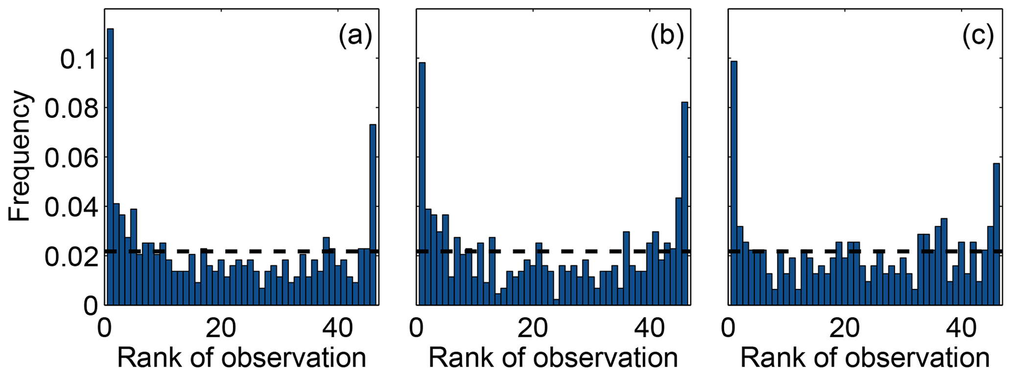
Figure 6Rank histogram of the 45-member ensemble for wind speed (a), wind direction (b) and PBLH (c) using 14 rawinsonde sites available over the region. The horizontal dashed line corresponds to the ideal value for a flat rank histogram with respect to the number of members.

Figure 7Spread–skill relationship for (a) wind speed, (b) wind direction and (c) PBLH using the 14 rawinsonde sites available over the region. Each point represents the model ensemble spread (standard deviation of the model–data difference) and skill (mean absolute error) for each observation. A one-to-one line is plotted in black and a line of best fit is plotted in red. Correlation (r) and slope (b) of the line of best fit of the spread–skill relationship are plotted as well.
Figure 7 shows the spread–skill relationship, another method that we use to examine the representation of errors of the ensemble. Wind direction (Fig. 7b) shows a higher correlation between the spread and the skill compared to the PBLH (Fig. 7c) and the wind speed (Fig. 7a). Therefore, the ensemble has a wider spread when the model–data differences are larger. The PBLH and wind speed show consistently poorer skill (a large mean absolute error) compared to their spread. This supports the conclusion that the large ensemble is underdispersive for these variables. None of these variables show a correlation equal to 1; this implies that our ensemble spread does not match exactly the atmospheric transport errors on a day-to-day basis. This feature is common among ensemble prediction systems (Wilks et al., 2011) and should not impair the ability to identify the optimal reduced-size ensembles.
3.2 Calibrated ensemble
In this section, we show the results of the calibrated ensembles generated with both SA and GA. Each calibration was performed for three different sub-ensemble sizes; the size of the ensembles is determined using the technique explained in Sect. 2.4. To compute the size of the sub-ensemble, we use the maximum frequency of the rank histogram using the large ensemble (Fig. 6). In this case, the maximum frequency is the left bar (r0) of every rank histogram. This technique yields the result that the calibrated ensemble should have about 8–10 members depending in the variable to be used. Therefore, for this study, we will generate 10-, 8- and 5-member ensembles using the two calibration techniques.
3.2.1 Individual variable calibration
Table 3 shows that both techniques (i.e., SA and GA) were able to find similar combinations of model configurations (i.e., an ensemble that shares more than half of the members) when each meteorological variable was used separately. The configurations chosen for each sub-ensemble vary significantly across the different variables, with the exception of the 10-member ensemble calibrated using wind speed and wind direction. The majority of the ensembles include model configuration 14. This model configuration, as shown in Díaz-Isaac et al. (2018), introduces large errors for both wind speed and wind direction, and is selected to allow for sufficient spread of these variables in the sub-ensembles. The final scores of the calibrated ensembles for each variable show that finding a calibrated sub-ensemble that reaches a score of 1 is not possible for wind speed and wind direction. A sub-ensemble with a score less than or equal to 1 can be found for PBLH. Figure 8 shows the rank histograms of the different calibrated ensembles (i.e., 10, 8 and 5 members) for each meteorological variable shown in Table 3. The calibrated ensembles of PBLH (Fig. 8c, f, i) are nearly flat for all ensemble sizes, whereas the 10- and 8-member sub-ensembles keep a slight U shape for wind speed and wind direction but are significantly flatter than the original ensemble. The ratio between the expected and observed frequency of the end members is reduced from 5 (original expected frequency of 0.02 with 0.1 frequency observed) to less than 2 (calibrated expected frequency of 0.1 with 0.15 frequency observed). The smallest rank-histogram scores for wind speed and wind direction are obtained with a five-member ensemble (Fig. 8g–h). The biases for all sub-ensembles (Table 3) are similar to or less than the bias of the large ensemble (Table 2).
Table 3Calibrated ensembles generated by both SA and GA and their rank-histogram scores and bias for each variable.
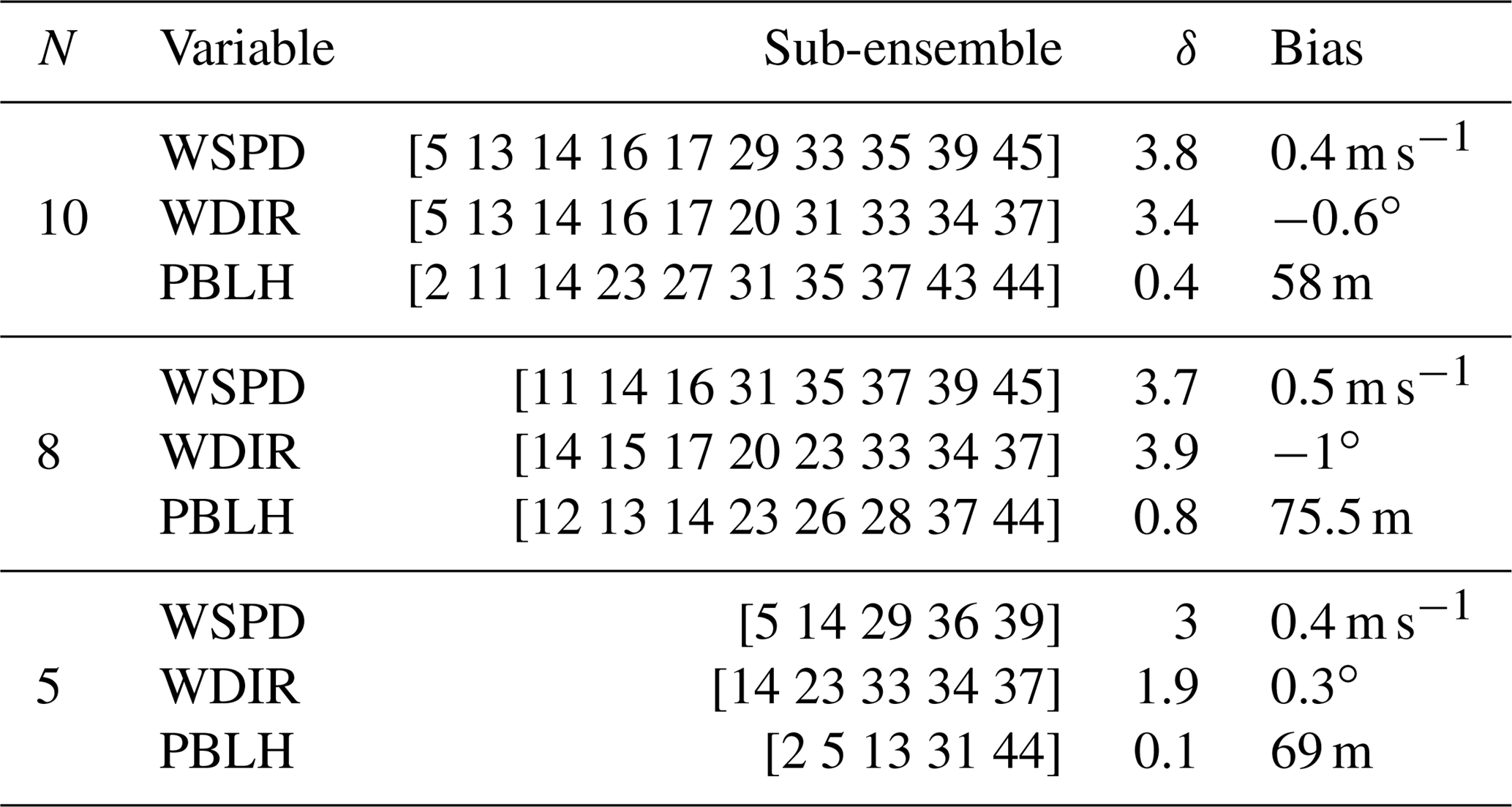
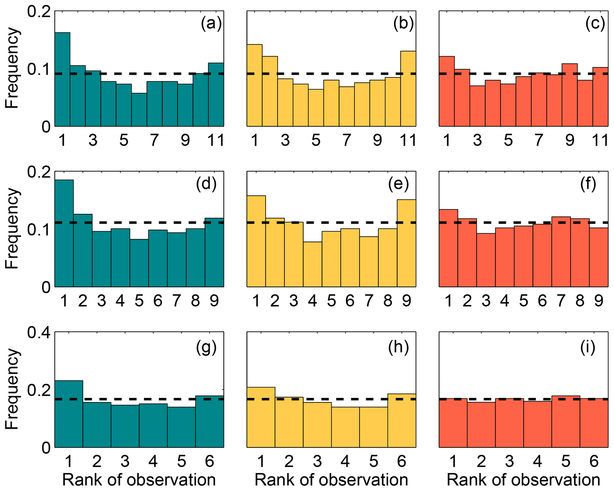
Figure 8Rank histograms of the calibrated ensembles found for wind speed (a, d, g), wind direction (b, e, h) and PBLH (c, f, i) for each of the ensemble size. The upper, middle and lower panels correspond to the ensembles with 10, 8 and 5 members, respectively. The horizontal dashed line corresponds to the ideal value for a flat rank histogram with respect to the number of members.
3.2.2 Multiple-variable calibration
Table 4 shows the sub-ensembles selected by SA. Each of the sub-ensembles has two simulations in common (i.e., 17 and 33), implying that these models are crucial to build an ensemble that best represents the transport errors for the three variables. Figure 9 shows the rank histograms of the sub-ensembles shown in Table 4. These rank histograms show that we were able to flatten the histogram relative to the 45-member ensemble for all three meteorological variables. Similar to the individual variable calibration, the rank histograms for wind speed (Fig. 9a, d) and wind direction (Fig. 9b, e) still show a U shape which is minimized for the smallest (i.e., five-member) sub-ensemble (Fig. 9g–h). The rank histograms are flatter for the PBLH (Fig. 9c, f, i) and the histogram score is closer to 1 (Table 4) compared to wind speed and wind direction. The rank-histogram scores for all variables are greater than those for one-variable optimization (see Table 4). The high rank-histogram scores are associated with the equal weight given to the three variables for this simultaneous calibration, where wind speed controlled the calibration process. For the calibration of the three variables together, we were not able to produce an ensemble for wind speed with a score smaller than 4; this ends up limiting the selection of the calibrated ensemble for the rest of the variables (see Fig. A4 in the Appendix). In addition, all these calibrated sub-ensembles have biases smaller in magnitude than the 45-member ensemble. Both wind speed and PBLH retain an overall positive bias, and wind direction a negative bias. The standard deviations of these three calibrated ensembles are larger than those of the large ensemble, consistent with the effort to increase the ensemble spread.
Table 4Ensemble members, rank-histogram scores (δ), bias and standard deviation (σ) for wind speed, wind direction and PBLH for the calibrated sub-ensembles generated with SA.
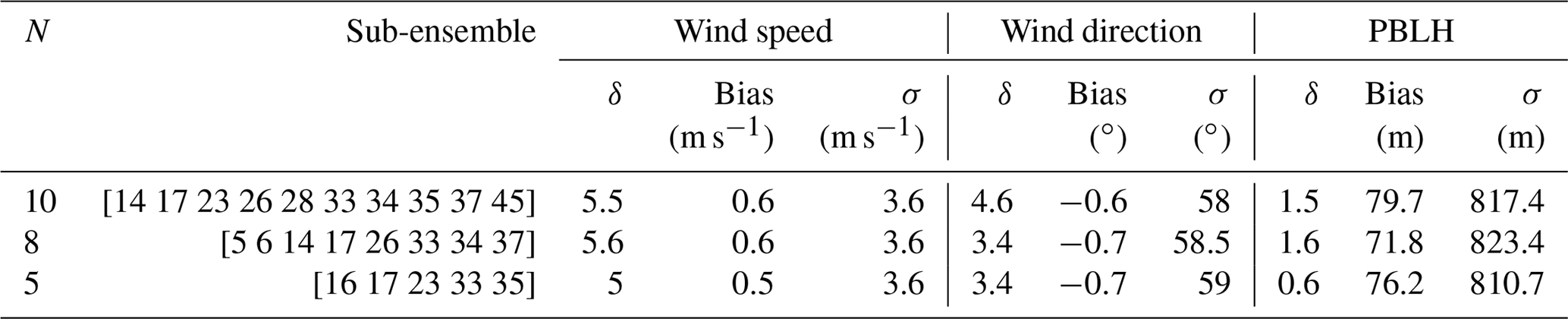
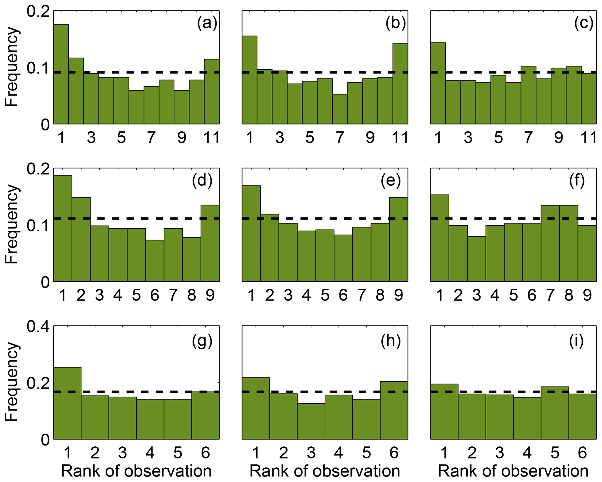
Figure 9Rank histograms of wind speed (a, d, g), wind direction (b, e, h) and PBLH (c, f, i) using the calibrated ensembles found with SA. The upper, middle and upper lower panels correspond to the ensembles with 10, 8 and 5 members, respectively. The horizontal dashed line corresponds to the ideal value for a flat rank histogram with respect to the number of members.
Using SA and GA techniques and the selection criteria detailed in Sect. 2.7 (i.e., low mean error of the entire ensemble), we defined an optimal five-member sub-ensemble (the optimal solution using both techniques) and nearly identical combinations of members for 10-and 8-member sub-ensembles, with only two model configurations not being shared by both algorithms. We also find that configuration 14 remains important for the multi-variable calibrated ensembles, as it was for the single-variable calibrated ensembles.
3.2.3 Evaluation of the multiple-variable calibrated ensemble
Both optimization techniques were able to generate sub-ensembles that reduce the U shape of the rank histograms, while significantly decreasing the number of members in the ensemble. A flatter histogram indicates that the ensemble is more reliable (unbiased) and has a more appropriate (greater) spread. The correlation between spread and skill for the wind direction increased, while wind speed and PBLH remain similar. Therefore, we conclude that the calibrated sub-ensembles are equivalent to or even better than the full ensemble to represent the daily model errors.
Figure 10Time series of simulated and observed 300 m wind speed (a–c), 300 m wind direction (d–f) and PBLH (g–i) using the 5-, 8- and 10-member calibrated ensembles (first, second and third columns, respectively) at the TOP rawinsonde site. The green shaded area represents the spread (i.e., root mean square deviation) of the ensemble, the black line is the mean of the ensemble, and the red dots are the observations at 00:00 UTC.
Figure 10 shows the time series of the different calibrated ensembles generated by the SA algorithm at the TOP site. In general, there are no major differences among 5- (Fig. 10a, d, g), 8- (Fig. 10e, h) and 10-member (Fig. 10c, f, i) ensembles. Figure 12 shows how the calibration can increase the spread of the ensemble to the extent of encompassing the observations (e.g., DOY 179; Fig. 10b–c) compared to the full ensemble (Fig. 5b). The ensemble spread was reduced after calibration at a few specific points in space and time.
Insight into the physics parameterizations can be gained by evaluating the calibrated ensembles. The LSM, PBL, CP and MP schemes, and reanalysis choice vary across all of the sub-ensemble members; no single parameterization is retained for all members in any of these categories. However, we also find that the calibrated ensembles rely upon certain physics parameterizations more than others. Figure 11 shows that most of the simulations in the calibrated ensemble use the RUC and thermal diffusion (T-D) LSMs in preference to the Noah LSM. In addition, more simulations use the MYJ PBL scheme than the other PBL schemes. The physics parameterizations shown with a higher percentage in Fig. 11 appear to contribute more to the spread of the ensemble than the other parameterizations.
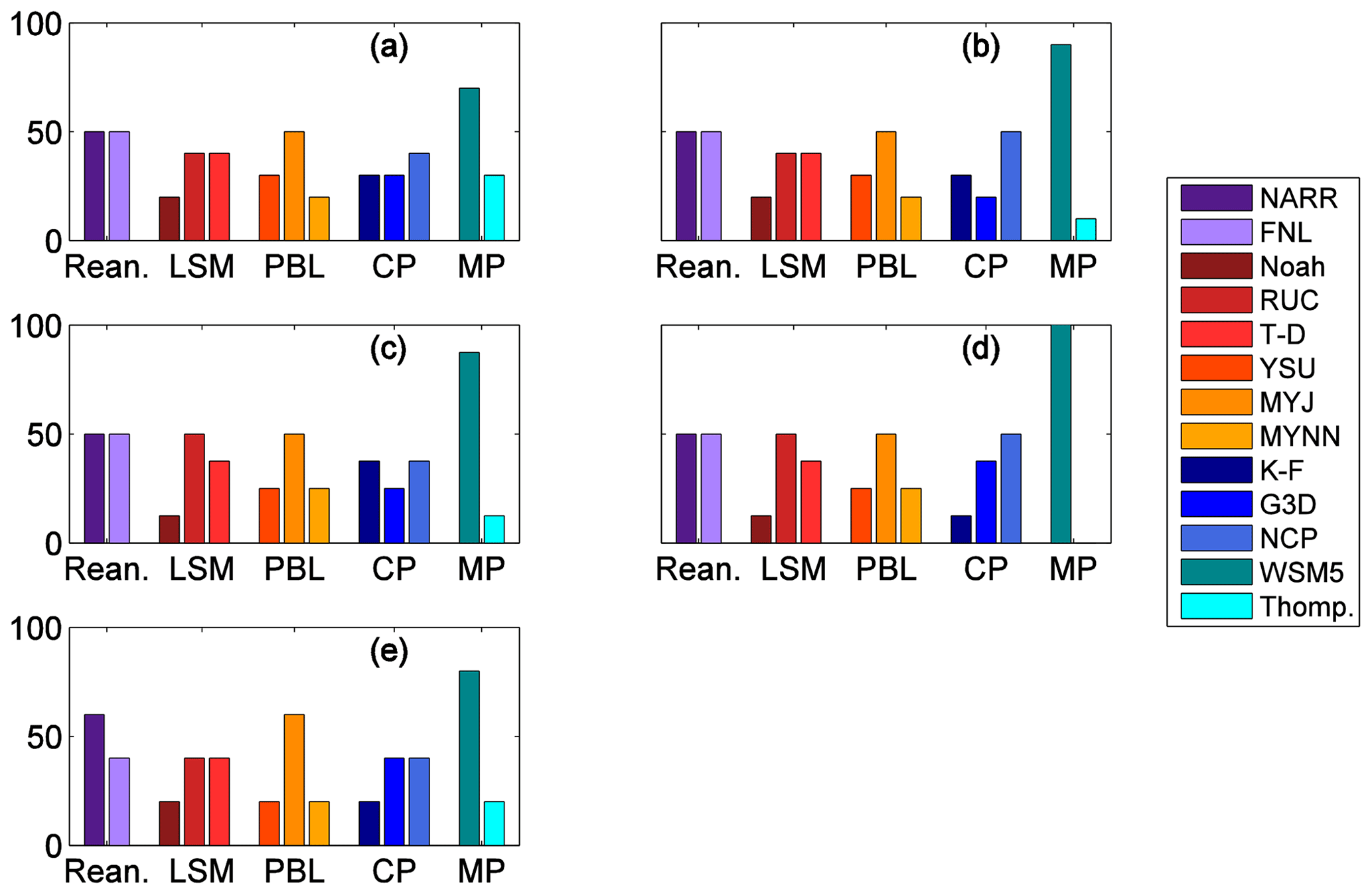
Figure 11Frequency with which the physics schemes are used for the SA (a, c, e) and GA (b, d, e) calibrated ensembles of 10 members (a, b), 8 members (c, d) and 5 members (e).
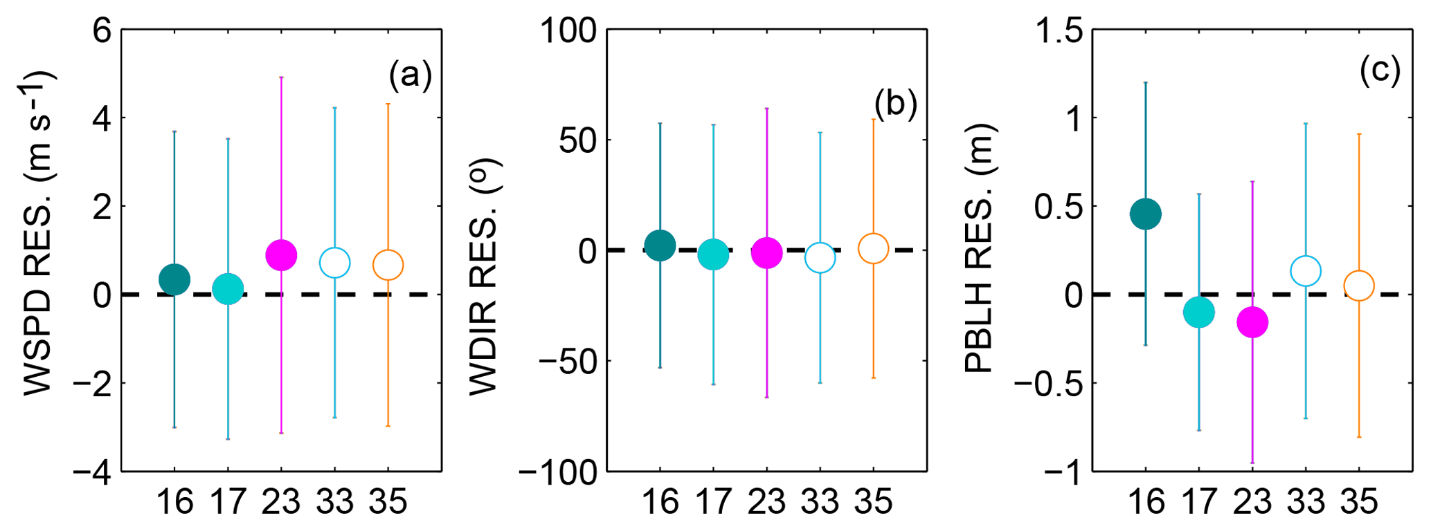
Figure 12Residual (model–data mismatch) mean and standard deviation of individual members for wind speed (a), wind direction (b) and PBLH (c) using the SA- and GA-calibrated sub-ensemble of five members.
We next explore the characteristics of the individual ensemble members that are retained in an effort to understand what member characteristics are important to increase the spread of the ensemble. Figure 12 shows the mean and standard deviation of the residuals for each simulation included in the five-member ensemble of SA and GA. Ensembles appear to need at least one member with a larger standard deviation to improve the spread for wind speed and wind directions (see member 23; Fig. 12a–b). Additionally, a member that has a large PBLH bias (see member 16; Fig. 12c) appears to be selected, highlighting the need for end members among the model configurations in order to reproduce the observed variability in PBLH. We note here that model configuration 14 was not selected when calibrating three variables together.
3.3 Propagation of transport uncertainties into CO2 concentrations
The calibrated ensembles found in this study were chosen based on the meteorological variables and not on the CO2 mole fractions to avoid the propagation of CO2 flux biases into the solution. We can now propagate these uncertainties, represented by the ensemble spread, into the CO2 concentration space. This straightforward calculation is possible because every model simulation uses identical CO2 fluxes. We present here the transport errors in both time and space with the spread in CO2 mole fractions, comparing the initial (uncalibrated) 45-member ensemble to the calibrated sub-ensembles.
3.3.1 CO2 error variances
Figure 13 shows the spread of daily daytime average CO2 mole fractions across the different sub-ensemble sizes at Mead (Fig. 13a, d, g, j), West Branch (Fig. 13b, e, h, k) and WLEF (Fig. 13c, f, i, l). The spread of the DDA CO2 mole fractions of the large ensemble (Fig. 13a–c) does not appear to differ in a systematic fashion from the spread of the calibrated small-size ensembles (Fig. 13d–l). While the calibration has increased the average ensemble spread, none of the ensembles consistently encompass the observations, either in terms of meteorological variables (Fig. 12) or CO2 (Fig. 15). The CO2 differences between the models and the observations may be caused by CO2 flux or boundary condition errors, the two components impacting the modeled CO2 mole fractions in addition to atmospheric transport. The cause of the total difference cannot be determined from the CO2 data alone. The increased daily variance in CO2 resulting from the ensemble calibration process is shown in Fig. 14. The eight-member ensemble often has the maximum CO2 variance. Table 5 shows the spread (model–ensemble mean) and RMSE (model–data) ratio of the CO2 mole fraction for the full and calibrated 10-member ensembles at each in situ CO2 observation tower. The ratio of the variances is an estimate of the contribution of the transport uncertainties to the CO2 model–data mismatch for the summer of 2008. This table shows that the transport uncertainties represent about 20 % to 40 % of the CO2 model–data mismatch. We found that values after calibration show a slight increase compared to the full ensemble.
Table 5Spread (model–ensemble mean), RMSE (model–data) and ratio (spread2/RMSE2) at each of the in situ CO2 mixing ratio towers, for the 45-member ensemble and 10-member ensemble calibrated with SA and GA.
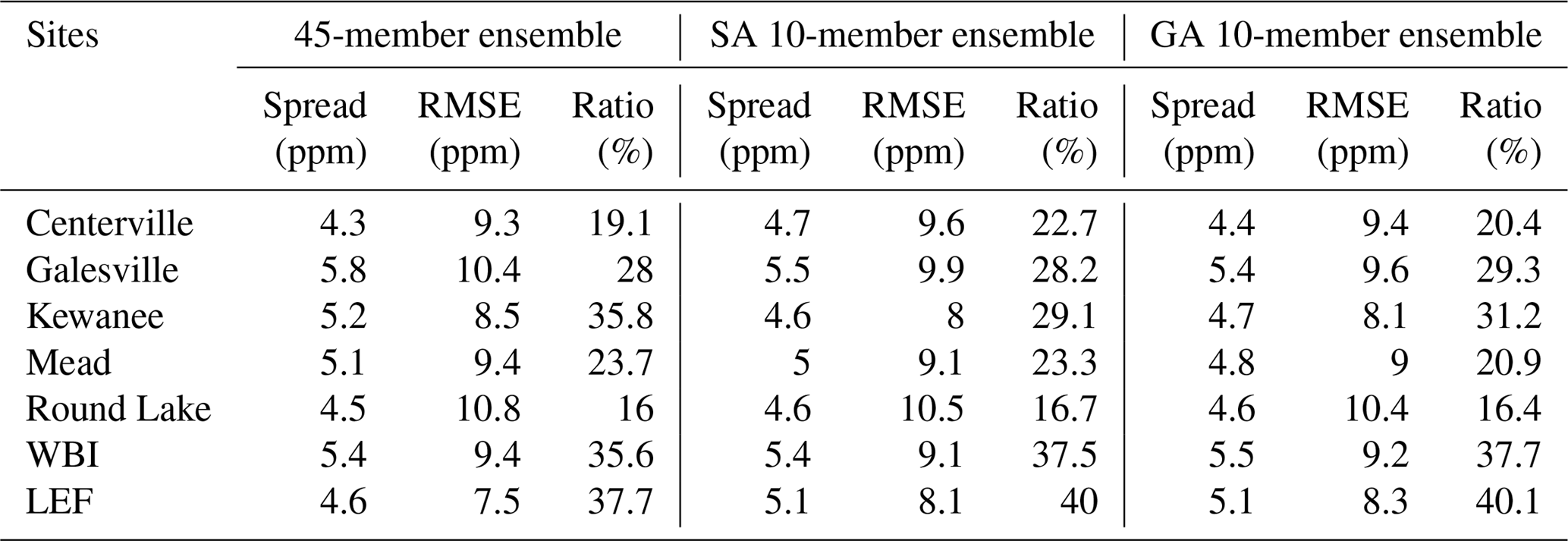
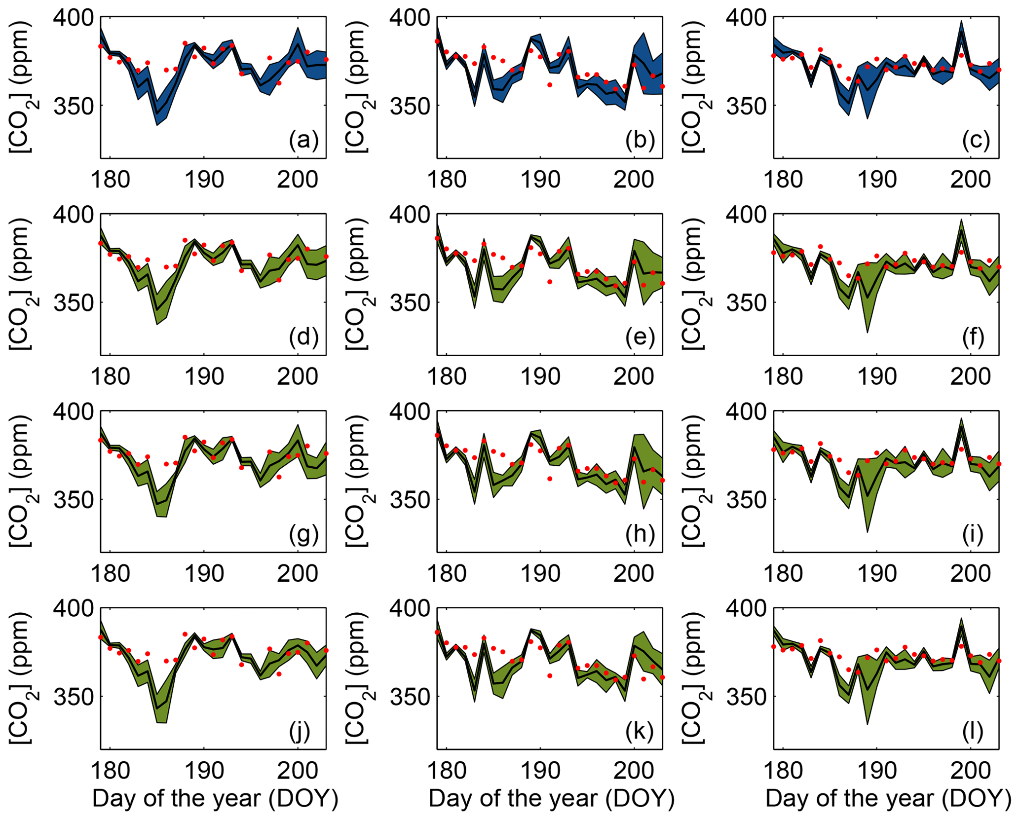
Figure 13Ensemble mean and spread (i.e., RMSD) of the DDA at approximately 100 m CO2 concentrations at Mead (first column; a, d, g, j), WBI (middle column; b, e, h, k) and WLEF (last column; c, f, i, l) towers using SA-calibrated ensembles. Rows from top to bottom are 45-, 10-, 8- and 5-member ensembles. The blue area is the spread of the 45-member ensemble, the green area is the spread is the spread of the calibrated (10-, 8- and 5-member) ensembles, the black line is the mean of the ensemble, and the red dots are the observations.
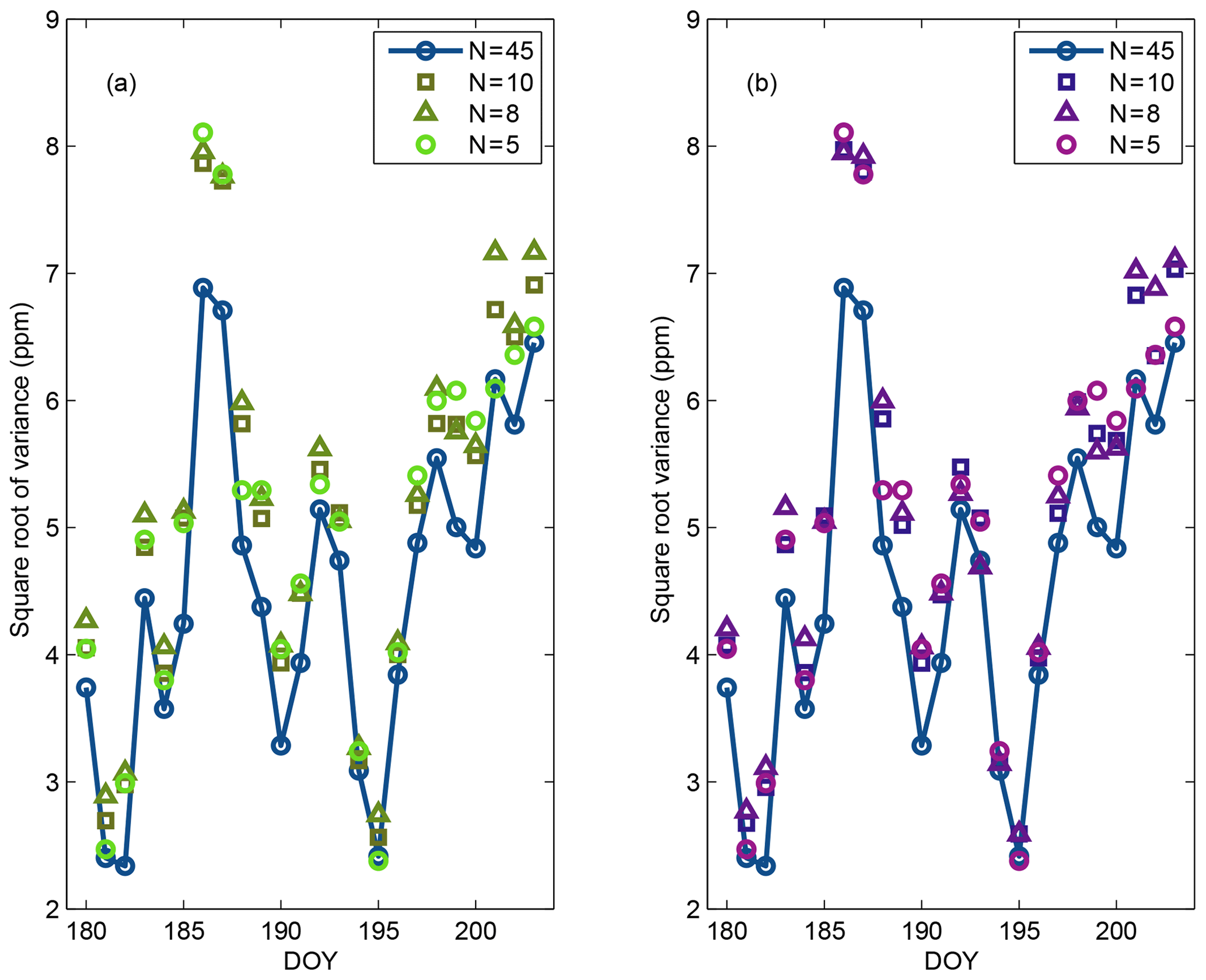
Figure 14Sum of the CO2 mixing ratio variance of the large (45-member) ensemble and the different sub-ensembles selected with the SA (a) and GA (b) down-selection techniques.
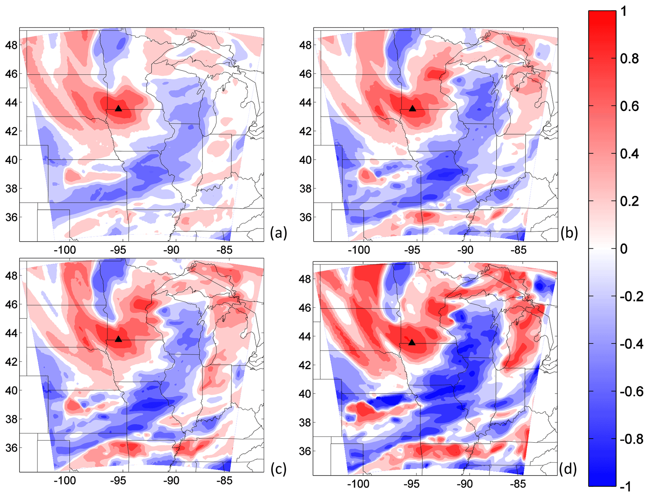
Figure 15Spatial correlation of CO2 for the 45- (a), 10-(b), 8- (c) and 5-member (d) ensembles with respect to the location of the Round Lake tower for DOY 180. This figure uses the calibrated ensembles of 10, 8 and 5 members found by the SA technique.
4.1 Impact of calibration on ensemble statistics
The calibration of the multi-physics/multi-analysis ensemble using SA and GA optimization techniques generated 10-, 8- and 5-member ensembles with a better representation of the error statistics of the transport model than the initial 45-member ensemble. One of our goals was to find sub-ensembles that fulfil the criteria of Sect. 2.7, independent of the selection algorithm and for multiple meteorological variables. Wind speed and wind direction statistics only improve by a modest amount in the calibrated ensembles as compared to the 45-member ensemble, while PBLH statistics, namely the flatness of the rank histogram, show a significant improvement in the calibrated ensembles. The variance in the calibrated ensembles increased relative to the 45-member ensemble but the potential for improvement was limited by the spread in the initial ensemble. Stochastic perturbations (e.g., Berner et al., 2009) could increase the spread of the initial ensemble, which, combined with the suite of model configurations, could better represent the model errors. Here, we limited the 45-member ensemble to mass-conserved, continuous flow (i.e., unperturbed) members that can be used in a regional inversion. Future work should address the problem of using an underdispersive ensemble before the calibration of the ensemble.
4.2 Single-variable and multiple-variable ensembles
We first attempted to calibrate the ensemble for each meteorological variable (i.e., wind speed, wind direction and PBLH). Table 3 shows that the different sub-ensembles were able to follow the criteria presented in Sect. 2.7, but the calibration of the single-variable ensembles did not allow us to find a unique sub-ensemble that can be used to represent the errors of the three variables. Therefore, the joint optimization of the three variables was required to identify an ensemble that best represents model errors across the three variables. By minimizing the sum of the squared rank-histogram scores of the three variables, the selection algorithm found common solutions at the expense of less satisfactory rank-histogram scores than were obtained for single-variable ensembles (see Table 4). We assumed that each variable was equally important to the problem, an assumption that has not been rigorously evaluated. Future work on the relative importance of meteorological variables on CO2 concentration errors would help weigh the scores in the selection algorithms.
4.3 Resolution and reliability
The calibrated ensembles show the rank-histogram score closer to 1 (Table 4), that is, flatter rank histograms (Fig. 9) compared to the 45-member ensemble (Table 2 and Fig. 6). The sub-ensembles do have a greater variance than the large ensemble (i.e., improved reliability) (Fig. 14). However, the spread–skill relationship (i.e., resolution) of the calibrated ensembles do not show any major improvement compared to the 45-member ensemble, implying that the spread of the ensemble does not represent the day-to-day transport errors well. While the rank histogram suggests that the different calibrated ensembles have enough spread, the spread–skill relationship indicates that our ensemble does not systematically encompass the observations. The disagreement between the rank histogram and the spread–skill relationship can be associated with the metric used for the calibration (i.e., rank histogram) and the biases included in the calibrated ensemble. Using the score of the rank histogram alone may not be sufficient to measure the reliability of the ensemble (Hamill, 2001); therefore, future down-selection studies should incorporate the resolution as part of the calibration process (skill score optimization). The biases in the model are a complex problem because there are many sources systematic errors within an atmospheric model (e.g., physical parameterizations and meteorological forcing). Future studies should consider data assimilation or improvement of the physics parameterizations to reduce or remove these systematic errors. To improve the representation of daily model errors, additional metrics should be introduced and the initial ensemble should offer a sufficient spread, possibly with additional physics parameterizations, additional random perturbations, or modifications of the error distribution of the ensemble (Roulston and Smith, 2003).
4.4 Error correlations
Rank histograms, as explained in Sect. 2.3.1, evaluate the ensemble by ranking individual observations in a relative sense. The ensembles calibrated using the rank histograms may be representing the variances over the region correctly but not the spatial and temporal structures of the errors (Hamill, 2001). These parameters are critical to inform regional inversions of correlations in model errors, directly impacting flux corrections (Lauvaux et al., 2009). In this study, the calibrated ensembles show an improvement in the meteorological variances and an increase in the CO2 variances relative to the uncalibrated ensemble. However, spatial structures of the errors were not evaluated and may be impacted by sampling noise. Few members will produce a statistically limited representation of the model error structures. For example, ensemble model prediction systems use at least 50 members to avoid sampling noise and correctly represent time and space correlations. Figure 15 shows the spatial correlation of 300 m DDA CO2 errors with respect to the Round Lake site on DOY 180. Error correlations increase significantly as our ensemble size decreases. With fewer members, spurious correlations increase, resulting in high correlations at long distances. Assuming we sample only a few times the distribution of errors, our ensemble is very likely to be affected by spurious correlations with a variance on the order of 1∕N. We conclude here that our reduced-size ensembles are impacted by sampling noise which would require additional filtering. Previous studies have suggested objective methods to filter the noise in small-size ensembles (i.e., Ménétrier et al., 2015) or modeling the error structures using the diffusion equation (e.g., Lauvaux et al., 2009). Future work should address the impact of the calibration on the error structures as this information is critical in the observation error covariance to assess the inverse fluxes. Concerning the magnitudes of the error correlation, the calibrated sub-ensembles exhibit a larger contrast in correlation values compared to the 45-member error correlations. Overall, the different ensembles show similar flow-dependent spatial patterns which demonstrates that the calibration process, even if generating sampling noise, preserves the dominant spatial patterns in the error structures. Therefore, the calibrated ensemble is likely to provide a better representation of the variances and a similar spatial error structure for the construction of error covariance matrices in regional inversions.
We applied a calibration (or down-selection) process to a multi-physics/multi-analysis ensemble of 45 members. In this calibration process, two optimization techniques were used to extract a subset of members from the initial ensemble to improve the representation of transport model uncertainties in CO2 inversion modeling. We used purely meteorological criteria to calibrate the ensemble and avoid contaminating the calibration with CO2 flux errors. The calibrated ensembles were optimized using criteria based on the flatness of the rank histogram. We generated different calibrated ensembles for three meteorological variables; PBL wind speed, PBL wind direction and PBLH. With these techniques, we identified sub-ensembles by calibrating the three variables jointly. Both techniques show that calibrated small-size ensembles can reduce the score of the rank-histogram flatness and therefore improve the representation of the model error variances with few members (between 5 and 10 members).
The calibration techniques improved the spread (flatness of the rank histogram) of the ensembles and slightly improved the biases, which were already small in the larger ensemble, but the calibration did not improve daily atmospheric transport errors as shown by the spread–skill relationship. We assessed how the calibrated ensemble errors propagate into the CO2 mole fractions simulated with identical CO2 fluxes (i.e., independent of the atmospheric conditions). The spread from the calibrated ensembles represented from 20 % to 40 % (Table 5) of the model–data 300 m DDA CO2 mismatches for summer 2008. These results suggest that additional errors in CO2 fluxes and/or large-scale boundary conditions represent a large fraction of the differences between modeled and observed CO2. Error correlations of the calibrated ensembles were compared to the large ensemble to identify any impact of the calibration. Compared to the initial error structures, the calibrated ensembles are most likely affected by sampling noise across the region, which suggests that additional filtering or modeling of the errors would be required in order to construct the error covariance matrix for regional CO2 inversion.
The code is accessible upon request by contacting the corresponding author (lzd120@psu.edu).
Meteorological data were obtained from the University of Wyoming's online data archive (http://weather.uwyo.edu/upperair/sounding.html, last access: 20 July 2018) for the 14 rawinsonde stations. The tower atmospheric CO2 concentration dataset is available online (https://doi.org/10.3334/ORNLDAAC/1202, Miles et al., 2013) from the Oak Ridge National Laboratory Distributed Active Archive Center, Oak Ridge, Tennessee, USA https://doi.org/10.3334/ORNLDAAC/1202 (Miles et al., 2013). The other two towers (Park Falls – WLEF; West Branch – WBI) are part of the Earth System Research Laboratory/Global Monitoring Division (ESRL/GMD) tall tower network (Andrews et al., 2014; https://www.esrl.noaa.gov/gmd/ccgg/insitu/, last access: 20 July 2018). The WRF model results are accessible upon request by contacting the corresponding author (lzd120@psu.edu).
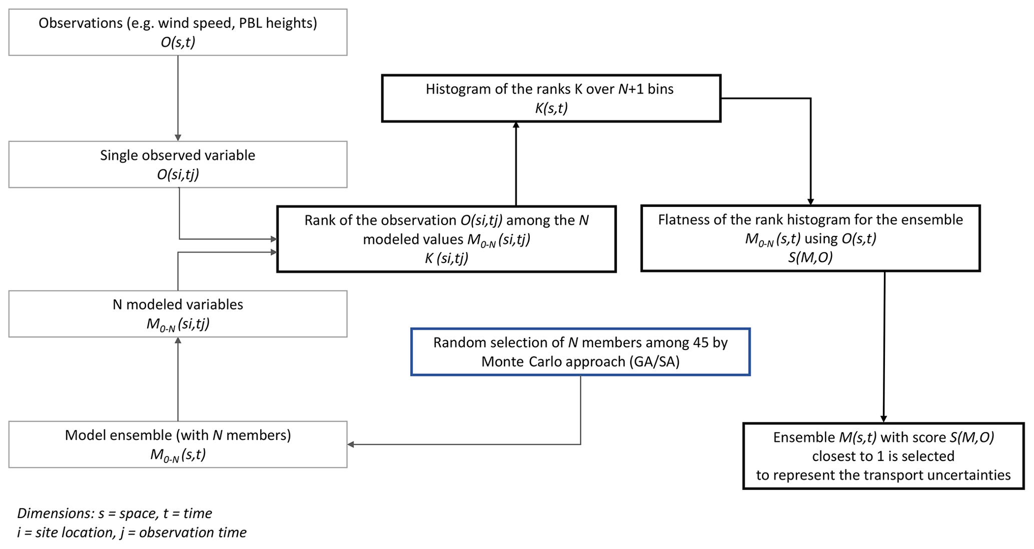
Figure A1Diagram of the rank-histogram process and selection of sub-ensembles based on the rank-histogram score.
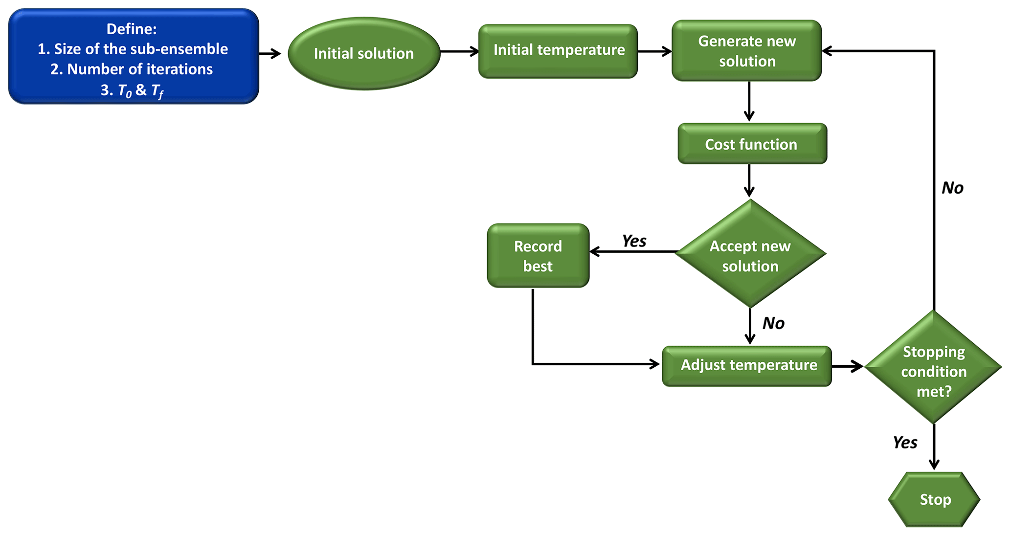

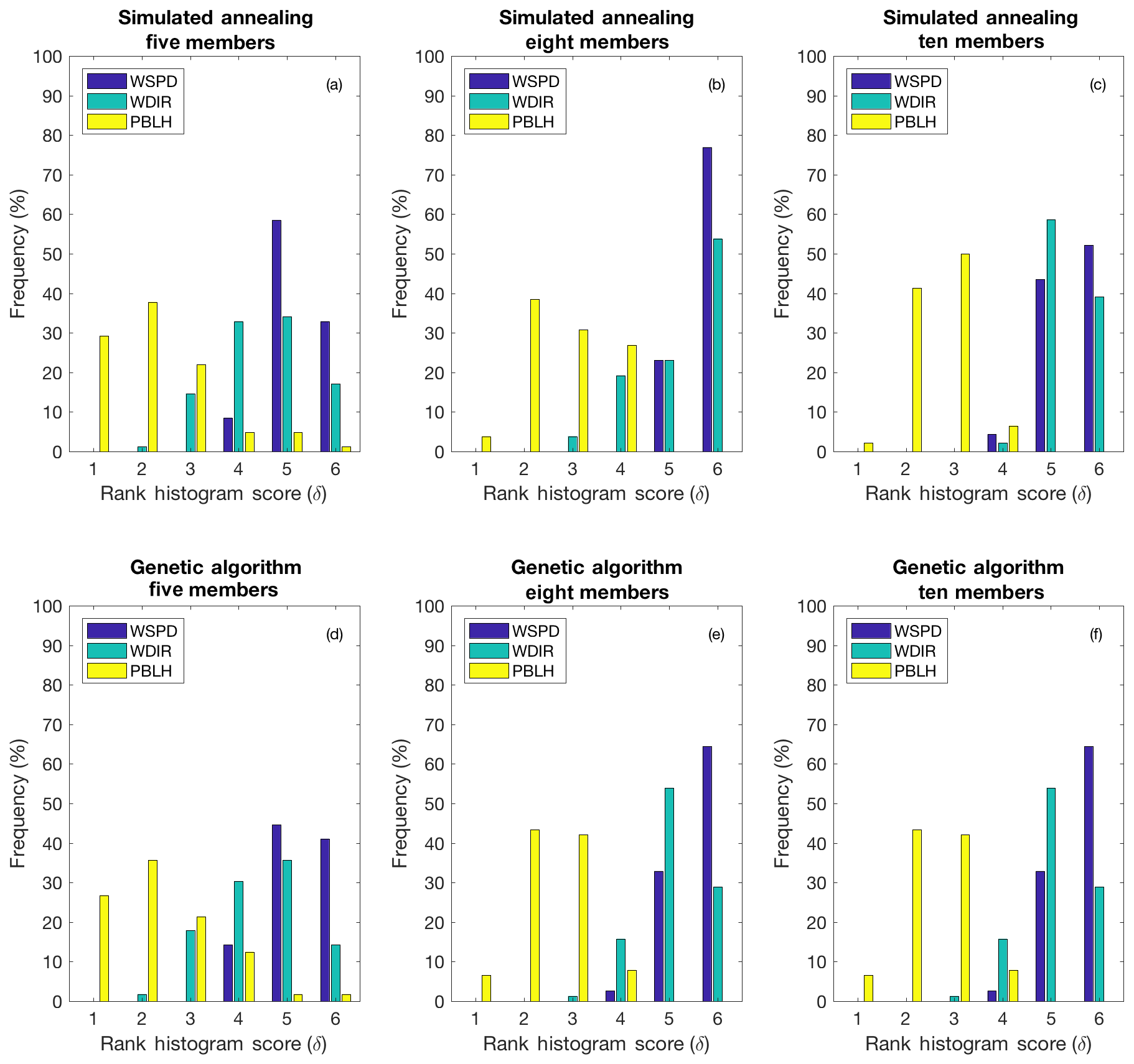
Figure A4Rank-histogram score of calibrated sub-ensembles of different size generated by simulated annealing (a–c) and the genetic algorithm (d–f). Each bar represents the frequency of that score for the three different variables: wind speed (WSPD), wind direction (WDIR) and PBL height (PBLH).
LDI performed the model simulations, calibration and the model–data analysis. The calibration technique was coded by MB, LDI and TL based on the work of Garaud and Mallet (2011). TL, MB and KJD provided guidance with the calibration and model–data analysis. All authors contributed to the design of the study and the preparation the paper.
The authors declare that they have no conflict of interest.
This research was supported by NASA's Terrestrial Ecosystem and Carbon Cycle Program (grant NNX14AJ17G), NASA's Earth System Science Pathfinder Program Office, Earth Venture Suborbital Program (grant NNX15AG76), NASA Carbon Monitoring System (grant NNX13AP34G) and an Alfred P. Sloan Graduate Fellowship. We thank Natasha Miles, Chris E. Forest and Andrew Carleton for fruitful discussions. Meteorological data used in this work were provided by University of Wyoming's online data archive (http://weather.uwyo.edu/upperair/sounding.html, last access: 12 July 2018). Observed atmospheric CO2 mole fraction was provided by the NOAA Earth System Research Laboratory (cited in the text) and PSU in situ measurement group (Miles et al., 2013).
This paper was edited by Marc von Hobe and reviewed by Lori Bruhwiler and Ian Enting.
Alhamed, A., Lakshmivarahan S., and Stensrud, D. J.: Cluster analysis of multimodel ensemble data from SAMEX, Mon. Weather Rev., 130, 226–256, https://doi.org/10.1175/1520-0493 (2002)130,0226:CAOMED.2.0.CO;2, 2002.
Anderson, J. L.: A method for producing and evaluating probabilistic forecasts from ensemble model integrations, J. Climate, 9, 1518–1530, https://doi.org/10.1175/1520-0442(1996)009<1518:AMFPAE>2.0.CO;2, 1996.
Andrews, A. E., Kofler, J. D., Trudeau, M. E., Williams, J. C., Neff, D. H., Masarie, K. A., Chao, D. Y., Kitzis, D. R., Novelli, P. C., Zhao, C. L., Dlugokencky, E. J., Lang, P. M., Crotwell, M. J., Fischer, M. L., Parker, M. J., Lee, J. T., Baumann, D. D., Desai, A. R., Stanier, C. O., De Wekker, S. F. J., Wolfe, D. E., Munger, J. W., and Tans, P. P.: CO2, CO, and CH4 measurements from tall towers in the NOAA Earth System Research Laboratory's Global Greenhouse Gas Reference Network: instrumentation, uncertainty analysis, and recommendations for future high-accuracy greenhouse gas monitoring efforts, Atmos. Meas. Tech., 7, 647–687, https://doi.org/10.5194/amt-7-647-2014, 2014.
Angevine, W. M., Brioude, J., McKeen, S., and Holloway, J. S.: Uncertainty in Lagrangian pollutant transport simulations due to meteorological uncertainty from a mesoscale WRF ensemble, Geosci. Model Dev., 7, 2817–2829, https://doi.org/10.5194/gmd-7-2817-2014, 2014.
Baker, D. F., Law, R. M., Gurney, K. R., Rayner, P., Peylin, P., Denning, A. S., Bousquet, P., Bruhwiler, L., Chen, Y. H., Ciais, P., Fung, I. Y., Heimann, M., John, J., Maki, T., Maksyutov, S., Masarie, K., Prather, M., Pak, B., Taguchi, S., and Zhu, Z.: TransCom 3 inversion intercomparison: Impact of transport model errors on the interannual variability of regional CO2 fluxes, 1988–2003, Global Biogeochem. Cy., 20, GB1002, https://doi.org/10.1029/2004GB002439, 2006.
Berner, J., Shutts, G. J., Leutbecher, M., and Palmer, T. N.: A Spectral Stochastic Kinetic Energy Backscatter Scheme and Its Impact on Flow-Dependent Predictability in the ECMWF Ensemble Prediction System, J. Atmos. Sci., 66, 603–626, https://doi.org/10.1175/2008JAS2677.1, 2009.
Buizza, R., Houtekamer, P. L., Pellerin, G., Toth, Z., Zhu, Y., and Wei, M.: A Comparison of the ECMWF, MSC, and NCEP Global Ensemble Prediction Systems, Mon. Weather Rev., 133, 1076–1097, https://doi.org/10.1175/MWR2905.1, 2005.
Candille, G. and Talagrand, O.: Evaluation of probabilistic prediction systems for a scalar variable, Q. J. Roy. Meteor. Soc., 131, 2131–2150, https://doi.org/10.1256/qj.04.71, 2005.
Černý, V.: Thermodynamical approach to the traveling salesman problem: An efficient simulation algorithm, J. Optim. Theory Appl., 45, 41–51, https://doi.org/10.1007/BF00940812, 1985.
Corbin, K. D., Denning, A. S., Lokupitiya, E. Y., Schuh, A. E., Miles, N. L., Davis, K. J., Richardson, S., and Baker, I. T.: Assessing the impact of crops on regional CO2 fluxes and atmospheric concentrations, Tellus B, 62, 521–532, https://doi.org/10.1111/j.1600-0889.2010.00485.x, 2010.
Crosby, J. L.: Computer Simulation in Genetics, John Wiley, Hoboken, N. J., 1973.
Davis, K. J., Bakwin, P. S., Yi, C., Berger, B. W., Zhao, C., Teclaw, R. M., and Isebrands, J. G.: The annual cycles of CO2 and H2O exchange over a northern mixed forest as observed from a very tall tower, Glob. Change Biol., 9, 1278–1293, https://doi.org/10.1046/j.1365-2486.2003.00672.x, 2003.
Denning, A. S., Fung, I. Y., and Randall, D.: Latitudinal gradient of atmospheric CO2 due to seasonal exchange with land biota, Nature, 376, 240–243, https://doi.org/10.1038/376240a0, 1995.
Díaz-Isaac, L. I., Lauvaux, T., Davis, K. J., Miles, N. L., Richardson, S. J., Jacobson, A. R., and Andrews, A. E.: Model-data comparison of MCI field campaign atmospheric CO2 mole fractions, J. Geophys. Res.-Atmos., 119, 10536–10551, https://doi.org/10.1002/2014JD021593, 2014.
Díaz-Isaac, L. I., Lauvaux, T., and Davis, K. J.: Impact of physical parameterizations and initial conditions on simulated atmospheric transport and CO2 mole fractions in the US Midwest, Atmos. Chem. Phys., 18, 14813–14835, https://doi.org/10.5194/acp-18-14813-2018, 2018.
Enting, I. G.: Inverse problems in atmospheric constituent studies: III, Estimating errors in surface sources, Inverse Probl., 9, 649–665, https://doi.org/10.1088/0266-5611/9/6/004, 1993.
Evensen, G.: Inverse Methods and Data Assimilation in Nonlinear Ocean Models, Phys. D Nonlinear Phenom., 77, 108–129, https://doi.org/10.1016/0167-2789(94)90130-9, 1994a.
Evensen, G.: Sequential data assimilation with a nonlinear quasi- geostrophic model using Monte Carlo methods to forecast error statistics, J. Geophys. Res., 99, 10143–10162, 1994b.
Feng, S., Lauvaux, T., Newman, S., Rao, P., Ahmadov, R., Deng, A., Díaz-Isaac, L. I., Duren, R. M., Fischer, M. L., Gerbig, C., Gurney, K. R., Huang, J., Jeong, S., Li, Z., Miller, C. E., O'Keeffe, D., Patarasuk, R., Sander, S. P., Song, Y., Wong, K. W., and Yung, Y. L.: Los Angeles megacity: a high-resolution land-atmosphere modelling system for urban CO2 emissions, Atmos. Chem. Phys., 16, 9019–9045, https://doi.org/10.5194/acp-16-9019-2016, 2016.
Fraser, A. and Burnell, D.: Computer Models in Genetics, McGraw-Hill, New York, 1970.
Garaud, D. and Mallet, V.: Automatic calibration of an ensemble for uncertainty estimation and probabilistic forecast: Application to air quality, J. Geophys. Res., 116, D19304, https://doi.org/10.1029/2011JD015780, 2011.
Gerbig, C., Lin, J. C, Wofsy, S. C., Daube, B. C., Andrews, A. E., Stephens, B. B., Bakwin, P. S., and Grainger, C. A.: Towards constraining regional-scale fluxes of CO2 with atmospheric observations over a continent: 1. Observed spatial variability from airborne platforms, J. Geophys. Res., 108, 4756, https://doi.org/10.1029/2002JD003018, 2003.
Gerbig, C., Körner, S., and Lin, J. C.: Vertical mixing in atmospheric tracer transport models: error characterization and propagation, Atmos. Chem. Phys., 8, 591–602, https://doi.org/10.5194/acp-8-591-2008, 2008.
Gourdji, S. M., Hirsch, A. I., Mueller, K. L., Yadav, V., Andrews, A. E., and Michalak, A. M.: Regional-scale geostatistical inverse modeling of North American CO2 fluxes: a synthetic data study, Atmos. Chem. Phys., 10, 6151–6167, https://doi.org/10.5194/acp-10-6151-2010, 2010.
Gurney, K. R., Law, R. M., Denning, A.S., Rayner, P. J., Baker, D., Bousquet, P., Bruhwiler, L., Chen, Y.-H., Ciais, P., Fan, S., Fung, I. Y., Gloor, M., Heimann, M., Higuchi, K., John, J., Maki, T., Maksyutov, S., Masarie, K., Peylin, P., Prather, M., Pak, B. C., Randerson, J., Sarmiento, J., Taguchi, S., Takahashi, T., and Yuen, C.-W.: Towards robust regional estimates of CO2 sources and sinks using atmospheric transport models, Nature, 415, 626–630, https://doi.org/10.1038/415626a, 2002.
Hamill, T. M.: Interpretation of rank histograms for verifying ensemble forecasts, Mon. Weather Rev., 129, 550–560, 2001.
Hamill, T. M. and Colucci, S. J.: Verification of Eta–RSM Short-Range Ensemble Forecasts, Mon. Weather Rev., 125, 1312–1327, https://doi.org/10.1175/1520-0493(1997)125<1312:VOERSR>2.0.CO;2, 1997.
Hilton, T. W., Davis, K. J., Keller, K., and Urban, N. M.: Improving North American terrestrial CO2 flux diagnosis using spatial structure in land surface model residuals, Biogeosciences, 10, 4607–4625, https://doi.org/10.5194/bg-10-4607-2013, 2013.
Holland J. H.: Adaptation in Natural and Artificial Systems, University of Michigan Press, Ann Arbor, 236 pp., 1975.
Hong, S.-Y., Noh, Y., and Dudhia, J.: A new vertical dif- fusion package with an explicit treatment of entrain- ment processes., Mon. Weather Rev., 134, 2318–2341, https://doi.org/10.1175/MWR3199.1, 2006.
Houtekamer, P. L. and Mitchell, H. L.: A Sequential Ensemble Kalman Filter for Atmospheric Data Assimilation, Mon. Weather Rev., 129, 123–137, https://doi.org/10.1175/1520-0493(2001)129<0123:ASEKFF>2.0.CO;2, 2001.
Houweling, S., Aben, I., Breon, F.-M., Chevallier, F., Deutscher, N., Engelen, R., Gerbig, C., Griffith, D., Hungershoefer, K., Macatangay, R., Marshall, J., Notholt, J., Peters, W., and Serrar, S.: The importance of transport model uncertainties for the estimation of CO2 sources and sinks using satellite measurements, Atmos. Chem. Phys., 10, 9981–9992, https://doi.org/10.5194/acp-10-9981-2010, 2010.
Huntzinger, D. N., Post, W. M., Wei, Y., Michalak, A. M., West, T. O., Jacobson, A. R., Baker, I. T., Chen, J. M., Davis, K. J., Hayes, D. J., Hoffman, F. M., Jain, A. K., Liu, S., McGuire, A. D., Neilson, R. P., Potter, C., Poulter, B., Price, D., Raczka, B. M., Tian, H. Q., Thornton, P., Tomelleri, E., Viovy, N., Xiao, J., Yuan, W., Zeng, N., Zhao, M., and Cook, R.: North American Carbon Program (NACP) regional interim synthesis: Terrestrial biospheric model intercomparison, Ecol. Model., 232, 144–157, https://doi.org/10.1016/J.Ecolmodel.2012.02.004, 2012.
Janjic, Z.: Nonsingular implementation of the Mellor-Yamada level 2.5 scheme in the NCEP Meso model, National Centers for En- vironmental Prediction, USA, Office Note No. 437, 2002.
Johnson, A., Wang, X., Xue, M., and Kong, F.: Hierarchical Cluster Analysis of a Convection-Allowing Ensemble during the Hazardous Weather Testbed 2009 Spring Experiment, Part II: Ensemble Clustering over the Whole Experiment Period, Mon. Weather Rev., 139, 3694–3710, https://doi.org/10.1175/MWR-D-11-00016.1, 2011.
Kirkpatrick, S., Gelatt, C. D., and Vecchi, M. P.: Optimization by Simulated Annealing, Science, 220, 671–680, https://doi.org/10.1126/science.220.4598.671, 1983.
Kretschmer, R., Gerbig, C., Karstens, U., and Koch, F.-T.: Error characterization of CO2 vertical mixing in the atmospheric transport model WRF-VPRM, Atmos. Chem. Phys., 12, 2441–2458, https://doi.org/10.5194/acp-12-2441-2012, 2012.
Lauvaux, T. and Davis, K. J.: Planetary boundary layer errors in mesoscale inversions of column-integrated CO2 measurements, J. Geophys. Res.-Atmos., 119, 490–508, https://doi.org/10.1002/2013JD020175, 2014.
Lauvaux, T., Pannekoucke, O., Sarrat, C., Chevallier, F., Ciais, P., Noilhan, J., and Rayner, P. J.: Structure of the transport uncertainty in mesoscale inversions of CO2 sources and sinks using ensemble model simulations, Biogeosciences, 6, 1089–1102, https://doi.org/10.5194/bg-6-1089-2009, 2009.
Law, R. M., Peters, W., Rödenbeck, C., Aulagnier, C., Baker, I., Bergmann, D. J., Bousquet, P., Brandt, J., Bruhwiler, L., Cameron-Smith, P. J., Christensen, J. H., Delage, F., Denning, A. S., Fan, S., Geels, C., Houweling, S., Imasu, R., Karstens, U., Kawa, S. R., Kleist, J., Krol, M. C., Lin, S. J., Lokupitiya, R., Maki, T., Maksyutov, S., Niwa, Y., Onishi, R., Parazoo, N., Patra, P. K., Pieterse, G., Rivier, L., Satoh, M., Serrar, S., Taguchi, S., Takigawa, M., Vautard, R., Vermeulen, A. T., and Zhu, Z.: TransCom model simulations of hourly atmospheric CO2: Experimental overview and diurnal cycle results for 2002, Global Biogeochem. Cy., 22, GB3009, https://doi.org/10.1029/2007GB003050, 2008.
Lee, J.: Techniques for Down-Selecting Numerical Weather Prediction Ensembles, Ph.D. Dissertation, The Pennsylvania State University, University Park, 131 pp., 2012.
Lee, J. A., Kolczynski, W. C., McCandless, T. C., and Haupt, S. E.: An Objective Methodology for Configuring and Down-Selecting an NWP Ensemble for Low-Level Wind Prediction, Mon. Weather Rev., 140, 2270–2286, https://doi.org/10.1175/MWR-D-11-00065.1, 2012.
Lee, J. A., Haupt, S. E. H. and Young, G. S.: Down-Selecting Numerical Weather Prediction Multi-Physics Ensembles with Hierarchical Cluster Analysis, J. Climatol. Weather Forecast., 4, 1–16, https://doi.org/10.4172/2332-2594.1000156, 2016.
Lin, J. C. and Gerbig, C.: Accounting for the effect of transport errors on tracer inversions, Geophys. Res. Lett., 32, 1–5, https://doi.org/10.1029/2004GL021127, 2005.
Ménétrier, B., Montmerle, T., Michel, Y., and Berre, L.: Linear Filtering of Sample Covariances for Ensemble-Based Data Assimilation, Part I: Optimality Criteria and Application to Variance Filtering and Covariance Localization, Mon. Weather Rev., 143, 1622–1643, https://doi.org/10.1175/MWR-D-14-00157.1, 2015.
Miles, N. L., Richardson, S. J., Davis, K. J., Lauvaux, T., Andrews, A. E., West, T. O., Bandaru, V., and Crosson, E. R.: Large amplitude spatial and temporal gradients in atmospheric boundary layer CO2 mole fractions detected with a tower-based network in the U.S. upper Midwest, J. Geophys. Res.-Biogeo., 117, 01019, https://doi.org/10.1029/2011JG001781, 2012.
Miles, N. L., Richardson, S. J., Davis, K. J., Andrews, A. E., Griffis, T. J., Bandaru, V., and Hosman, K. P.: NACP MCI: Tower Atmospheric CO2 Concentrations, Upper Midwest Region, USA, 2007–2009, Oak Ridge National Laboratory Distributed Active Archive Center, Oak Ridge, Tennessee, USA, https://doi.org/10.3334/ORNLDAAC/1202, 2013.
Miller, S. M., Hayek, M. N., Andrews, A. E., Fung, I., and Liu, J.: Biases in atmospheric CO2 estimates from correlated meteorology modeling errors, Atmos. Chem. Phys., 15, 2903–2914, https://doi.org/10.5194/acp-15-2903-2015, 2015.
Nakanishi, M. and Niino, H.: An improved Mellor-Yamada Level-3 model with condensation physics: Its design and verification, Bound.-Lay. Meteorol., 112, 1–31, https://doi.org/10.1023/B:BOUN.0000020164.04146.98, 2004.
Patra, P. K., Law, R. M., Peters, W., Rödenbeck, C., Takigawa, M., Aulagnier, C., Baker, I., Bergmann, D. J., Bousquet, P., Brandt, J., Bruhwiler, L., Cameron-Smith, P. J., Christensen, J. H., Delage, F., Denning, A. S., Fan, S., Geels, C., Houweling, S., Imasu, R., Karstens, U., Kawa, S. R., Kleist, J., Krol, M. C., Lin, S. J., Lokupitiya, R., Maki, T., Maksyutov, S., Niwa, Y., Onishi, R., Parazoo, N., Pieterse, G., Rivier, L., Satoh, M., Serrar, S., Taguchi, S., Vautard, R., Vermeulen, A. T., and Zhu, Z.: TransCom model simulations of hourly atmospheric CO2: Analysis of synoptic-scale variations for the period 2002-2003, Global Biogeochem. Cy., 22, GB4013, https://doi.org/10.1029/2007GB003081, 2008.
Peters, W., Jacobson, A. R., Sweeney, C., Andrews, A. E., Conway, T. J., Masarie, K., Miller, J. B., Bruhwiler, L. M. P., Pétron, G., Hirsch, A. I., Worthy, D. E. J., van der Werf, G. R., Randerson, J. T., Wennberg, P. O., Krol, M. C., and Tans, P. P.: An atmospheric perspective on North American carbon dioxide exchange: CarbonTracker, P. Natl. Acad. Sci. USA, 104, 18925–18930, https://doi.org/10.1073/pnas.0708986104, 2007.
Peylin, P., Law, R. M., Gurney, K. R., Chevallier, F., Jacobson, A. R., Maki, T., Niwa, Y., Patra, P. K., Peters, W., Rayner, P. J., Rödenbeck, C., van der Laan-Luijkx, I. T., and Zhang, X.: Global atmospheric carbon budget: results from an ensemble of atmospheric CO2 inversions, Biogeosciences, 10, 6699–6720, https://doi.org/10.5194/bg-10-6699-2013, 2013.
Pickett-Heaps, C. A., Rayner, P. J., Law, R. M., Ciais, P., Patra, P. K., Bousquet, P., Peylin, P., Maksyutov, S., Marshall, J., Rödenbeck, C., Langenfelds, R. L., Steele, L. P., Francey, R. J., Tans, P., and Sweeney, C.: Atmospheric CO2 inversion validation using vertical profile measurements: Analysis of four independent inversion models, J. Geophys. Res.-Atmos., 116, 3773–3779, https://doi.org/10.1029/2010JD014887, 2011.
Riccio, A., Ciaramella, A., Giunta, G., Galmarini, S., Solazzo, E., and Potempski, S.: On the systematic reduction of data complexity in multimodel atmospheric dispersion ensemble modeling, J. Geophys. Res.-Atmos., 117, D05314, https://doi.org/10.1029/2011JD016503, 2012.
Richardson, S. J., Miles, N. L., Davis, K. J., Crosson, E. R., Rella, C. W., and Andrews, A. E.: Field testing of cavity ring-down spectroscopy analyzers measuring carbon dioxide and water vapor, J. Atmos. Ocean. Tech., 29, 397–406, https://doi.org/10.1175/JTECH-D-11-00063.1, 2012.
Roulston, M. S. and Smith, L. A.: Combining dynamical and statistical ensembles, Tellus A, 55, 16–30, https://doi.org/10.1034/j.1600-0870.2003.201378.x, 2003.
Sarmiento, D. P., Davis, K. J., Deng, A., Lauvaux, T., Brewer, A., and Hardesty, M.: A comprehensive assessment of land surface-atmosphere interactions in a WRF/Urban modeling system for Indianapolis, Elementa, 5, https://doi.org/10.1525/elementa.132, 2017.
Sarmiento, J. L., Gloor, M., Gruber, N., Beaulieu, C., Jacobson, A. R., Mikaloff Fletcher, S. E., Pacala, S., and Rodgers, K.: Trends and regional distributions of land and ocean carbon sinks, Biogeosciences, 7, 2351–2367, https://doi.org/10.5194/bg-7-2351-2010, 2010.
Schuh, A. E., Lauvaux, T., West, T. O., Denning, A. S., Davis, K. J., Miles, N., Richardson, S., Uliasz, M., Lokupitiya, E., Cooley, D., Andrews, A., and Ogle, S.: Evaluating atmospheric CO2 inversions at multiple scales over a highly inventoried agricultural landscape, Glob. Change Biol., 19, 1424–1439, https://doi.org/10.1111/gcb.12141, 2013.
Skamarock, W. C., Klemp, J. B., Dudhia, J., Gill, D. O., Barker, D. M., Duda, M., Huang, X. Y., Wang, W., and Powers, J. G.: A description of the advanced research WRF version 3, NCAR, Tech. Note, Mesoscale and Microscale Meteorology Division, National Center for Atmospheric Research, Boulder, Colorado, USA, 2008.
Solazzo, E. and Galmarini, S.: The Fukushima-137Cs deposition case study: Properties of the multi-model ensemble, J. Environ. Radioact., 139, 226–233, https://doi.org/10.1016/j.jenvrad.2014.02.017, 2014.
Stephens, B. B., Gurney, K. R., Tans, P. P., Sweeney, C., Peters, W., Bruhwiler, L., Ciais, P., Ramonet, M., Bousquet, P., Nakazawa, T., Aoki, S., Machida, T., Inoue, G., Vinnichenko, N., Lloyd, J., Jordan, A., Heimann, M., Shibistova, O., Langenfelds, R. L., Steele, L. P., Francey, R. J., and Denning, A. S.: Weak northern and strong tropical land carbon uptake from vertical profiles of atmospheric CO2, Science, 316, 1732–1735, https://doi.org/10.1126/science.1137004, 2007.
Stull, R. B.: An Introduction to Boundary Layer Meteorology, Kluwer Academic, Dordrecht, 666 pp., 1988.
Talagrand, O., Vautard, R., and Strauss, B.: Evaluation of Probabilistic Prediction System, in: Workshop on Predictability, ECMWF, Reading, U. K., 1999.
Taylor, K. E.: Summarizing multiple aspects of model performance in a single diagram, J. Geophys. Res., 106, 7183–7192, https://doi.org/10.1029/2000JD900719, 2001.
Thompson, G., Rasmussen, R. M., and Manning, K.: Explicit Forecasts of Winter Precipitation Using an Improved Bulk Micro- physics Scheme, Part I: Description and Sensitivity Analysis, Mon. Weather Rev., 132, 519–542, 2004.
Wang, W., Davis, K. J., Yi, C., Patton, E. G., Butler, M. P., Ricciuto, D. M., and Bakwin, P. S.: A note on top-down and bottom-up gradient functions over a forested site, Bound.-Lay. Meteorol., 124, 305–314, https://doi.org/10.1007/s10546-007-9162-0, 2007.
Whitaker, J. S. and Loughe, A. F.: The Relationship between Ensemble Spread and Ensemble Mean Skill, Mon. Weather Rev., 126, 3292–3302, https://doi.org/10.1175/1520-0493(1998)126<3292:TRBESA>2.0.CO;2, 1998.
Wilks, D. S.: Statistical Methods in the Atmospheric Sciences, 3rd edn., Academic Press, Oxford, Waltham, MA, 2011.
Williams, I. N., Riley, W. J., Torn, M. S., Berry, J. A., and Biraud, S. C.: Using boundary layer equilibrium to reduce uncertainties in transport models and CO2 flux inversions, Atmos. Chem. Phys., 11, 9631–9641, https://doi.org/10.5194/acp-11-9631-2011, 2011.
Yussouf, N., Stensrud, D. J., and Lakshmivarahan, S.: Cluster analysis of multimodel ensemble data over New England, Mon. Weather Rev., 132, 2452–2462, https://doi.org/10.1175/1520-0493(2004)132<2452:CAOMED>2.0.CO;2, 2004.
Yver, C. E., Graven, H. D., Lucas, D. D., Cameron-Smith, P. J., Keeling, R. F., and Weiss, R. F.: Evaluating transport in the WRF model along the California coast, Atmos. Chem. Phys., 13, 1837–1852, https://doi.org/10.5194/acp-13-1837-2013, 2013.