the Creative Commons Attribution 4.0 License.
the Creative Commons Attribution 4.0 License.
 | 08 Feb 2019
Retrieving the age of air spectrum from tracers: principle and method
Aurélien Podglajen
Felix Ploeger
Surface-emitted tracers with different dependencies on transit time (e.g., due to chemical loss or time-dependent boundary conditions) carry independent pieces of information on the age of air spectrum (the distribution of transit times from the surface). This paper investigates how and to what extent knowledge of tracer concentrations can be used to retrieve the age spectrum. Since the mixing ratios of the tracers considered depend linearly on the transit time distribution, the question posed can be formulated as a linear inverse problem of small dimension. An inversion methodology is introduced, which does not assume a prescribed shape for the spectrum. The performance of the approach is first evaluated on a constructed set of artificial radioactive tracers derived from idealized spectra. Hereafter, the inversion method is applied to outputs of a chemistry–transport model. The latter experiment highlights the limits of inversions using only parent radioactive tracers: they are unable to retrieve fine-scale structures such as the annual cycle. Improvements can be achieved by including daughter decaying tracers and tracers with an annual cycle at the surface. This study demonstrates the feasibility of retrieving the age spectrum from tracers and has implications for transport diagnosis in models and observations.
- Article
(4360 KB) - Full-text XML
- BibTeX
- EndNote


The transport of surface-emitted tracers strongly influences the composition and chemistry of the atmosphere, as well as the global radiative balance (Riese et al., 2012). In turn, radiatively active species affect the diabatic budget, eventually reshaping the circulation and thus the transport itself. For instance, climate models predict a strengthening of the stratospheric Brewer–Dobson circulation caused by increasing anthropogenic greenhouse gas emissions at the surface (Butchart et al., 2010).
To characterize transport from the surface to a given region of the atmosphere, a number of observational (e.g., Engel et al., 2009) and modeling studies have focused on the average transit time, the mean age of air. However, it has long been acknowledged that the description of transport provided by the mean age is incomplete (e.g., Hall and Plumb, 1994). Large- and small-scale turbulent motions lead to mixing, so that a given air parcel is a mixture of air masses with different paths and transit time from the surface (Waugh and Hall, 2002). Strictly, there is a frequency distribution of transit timescales for each air parcel, which is known in the stratospheric literature as the age spectrum (Hall and Plumb, 1994; Waugh and Hall, 2002), while the tropospheric literature more frequently uses the abbreviation TTD for transit time distribution (Holzer et al., 2003).
Considering the full age spectrum rather than the mean age allows one to separate among different transit times related to different pathways of transport and to disentangle their potentially contrasted evolutions with climate change (see Ploeger and Birner, 2016, and references therein). It also enables an improved understanding of the air composition in a number of species without restricting to inert, linearly increasing tracers (Schoeberl et al., 2000).
Until now, the stratospheric age spectrum has mainly been estimated in models, using either Lagrangian trajectories (e.g Reithmeier et al., 2008; Diallo et al., 2012) or a set of artificial pulse tracers initialized in the lowest model layer (Li et al., 2012; Ploeger and Birner, 2016). Only a handful of studies (Andrews et al., 1999; Johnson et al., 1999; Schoeberl et al., 2005) have attempted to infer the age spectrum from observed tracers, and all assumed either a given shape for the distribution or steadiness of the flow. Many tracers, however, bear the imprint of specific regions of the age spectrum (e.g., Waugh et al., 2003, 2013; Orbe et al., 2016) and, combined together, may provide information on the entire transit time distribution.
In this study, we propose a general methodology for retrieving the age spectrum from the concentrations of (non-pulse) tracers, which may undergo chemistry and have time-dependent sources. The basic idea is to consider the tracer contents as images of the age spectrum through a known forward model and to pose the retrieval of the age spectrum as an inverse problem. We demonstrate the feasibility of the method in a well-defined model environment and investigate its opportunities and limitations for different types of input tracers.
The article is organized as follows. Section 2 recalls the fundamentals of the theory behind the age spectrum, makes explicit its relation to tracer concentrations and reviews previous approaches used to infer the age spectrum from tracers. Then, Sect. 3 presents the proposed inversion methodology and evaluates it based on idealized age spectra and a set of artificial decaying tracers. In Sect. 4, the method is used on realistic age spectra from a chemistry–transport model, which motivates a discussion of its limitations and applicability to observable tracers. Finally, Sect. 5 provides the conclusions.
2.1 Lagrangian path distribution
In the Lagrangian view of atmospheric transport (large-scale advection and mixing), each air parcel can be conceptually1 decomposed into “an infinitude of infinitesimal and irreducible `fluid elements' that maintain their integrity against mixing for all timescales” (Waugh and Hall, 2002). To each fluid element corresponds one Lagrangian path connecting a source (located at a given position on a surface) and the air parcel. Note that for any given source and emission time there might be a number of Lagrangian paths and hence of fluid elements. Each fluid element then explains a fraction mk of the mass of the air parcel, so that the partition of fluid elements fulfills
Such a decomposition enables us to understand the properties of the air parcel by disentangling the relative contribution of air masses of different origins. For instance, let us consider the age τ of the air parcel (average transit time since leaving the surface Ω). This age of air can be broken down into the transit times τk of each of the fluid elements, with the relation
Similarly, for a tracer of mixing ratio χ, one formally may write
It should be noted here that the decomposition used in Eq. (3) is not meaningful for all tracers. Actually, Eq. (3) makes sense only if the evolution of χ due to chemistry (or any process other than transport) can also be decomposed as
where is the rate of change of χk within each of the k fluid elements, if they were separated (unmixed). In other words, does not depend on whether the fluid elements are mixed or remain isolated from one another. For instance, reactive chemical species involved in bimolecular reactions do not meet that requirement because their rate of change is, in general, affected by mixing (if the different fluid elements have different tracer concentrations). A simple example of tracers fulfilling the condition expressed by Eq. (4) is conserved tracers, for which . Another example is that of tracers whose loss or growth rate is a linear function of their concentration (Schoeberl et al., 2000), such as radioactive tracers or tracers subject to photochemical loss. Their mixing ratio verifies
with r and t representing an eventual dependency of the growth or decay coefficient λ on position and time (for photochemical loss). For a pool of n tracers, Eq. (5) can be generalized into
with χ the vector of trace species' mixing ratios and M(r,t) the matrix of growth–decay coefficients. In addition to the “parent” radioactive tracers of Eq. (5), Eq. (6) also encompasses the products of their decay (“daughter” tracers).
Being the frequency distribution of transit times τk for all fluid elements constitutive of the air parcel, the age spectrum can be viewed as a specific regrouping of Lagrangian paths according to transit time. It is also a boundary propagator of the continuity equation of conserved tracers from the surface Ω into the atmosphere (e.g., Holzer and Hall, 2000): in other words, the age spectrum relates the concentration of an inert tracer within the atmosphere to its uniform boundary condition on Ω. This result can be extended to include tracers undergoing radioactive or chemical loss, as shown by a number of studies (e.g., Schoeberl et al., 2000, 2005; Waugh et al., 2003). In the next subsection, we recall the analytical relations between age spectra and tracer content. This formal description will enable the reader to clearly apprehend the suitability of a given set of trace gas species to probe the age spectrum.
2.2 Relation between age spectrum and tracer content
2.2.1 From age spectrum to tracer content: the forward model
Assuming it has a uniform boundary condition in the surface region Ω and a constant decay rate λ, the mixing ratio ξ of a tracer may be expressed as (e.g., Waugh et al., 2003)
where τ is the transit time from Ω to (r,t) and ξΩ is the tracer concentration at the surface. Here, represents the distribution of transit times, i.e., the age spectrum, at time t and position r. In the following we will drop the explicit reference to r in order to simplify the notations. Equation (7) can be generalized to a vector equation for n different tracers (similar to our argument regarding Eq. 6):
where ξ is a vector of species mixing ratios, M is the matrix of growth–decay coefficients and eMτ is the matrix exponential of Mτ. Equation (8) may encompass parent radioactive tracers as well as the whole associated decay chain (primary, secondary, … decay products), as explained in more detail in Sect. 4.2. It should be mentioned here that the derivation of Eqs. (7) and (8) is based on the assumption of a constant lifetime 1∕λ. Although this assumption holds for radioactive tracers, the direct applicability of Eqs. (7) and (8) for the case of chemically active tracers is more questionable. This critical issue is discussed further in Sect. 4.3.
With the constant-lifetime assumption, Eqs. (7) and (8) show that the mixing ratio of any conserved or exponentially decaying (or growing) tracer may be expressed as the convolution of a generic function (involving time dependency of the source and chemistry) and the age spectrum G. The tracer content can hence be seen as a weighted average of the age spectrum, and the functions eMτ ξΩ(t−τ) as weighting functions (note that this perspective is reversed with respect to the general view that the age spectrum is a weighting function of the tracer boundary condition history modulated by the sink terms). However, although information on the age spectrum is contained in the tracer concentrations, it is far from being directly accessible because of this convolution with the tracer-dependent weighting functions. This limitation is evident in the case of linearly decaying tracers with a constant boundary condition at the surface and constant lifetimes . For those, Eq. (8) simplifies as
where, as noted by Schoeberl et al. (2000), is the Laplace transform of the age spectrum.2 The corresponding exponential weighting functions are represented in Fig. 1 for a pool of such tracers. They all peak for short transit times, so that the information provided by the different tracers is partly redundant and needs to be deconvolved. In general, this deconvolution may be achieved using different approaches, which will depend on the type of tracer considered and its associated weighting functions.
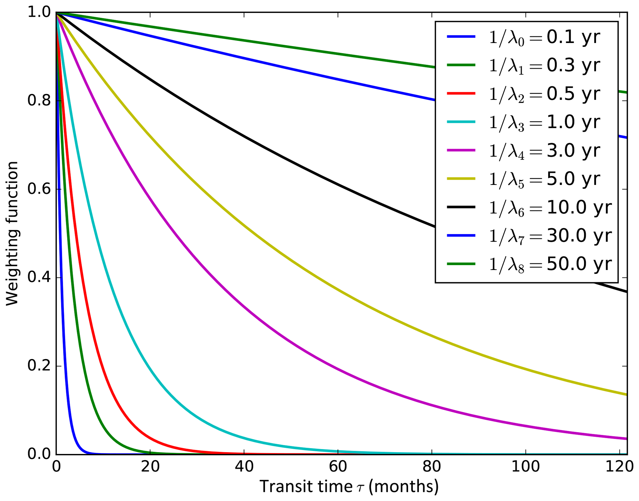
Figure 1Shape of the weighting function () to the age spectrum for exponentially decaying tracers with different lifetimes ranging from 0.1 to 50 years.
2.2.2 Diagnosing the age spectrum from the tracers: review of previous approaches
There have been a few attempts to characterize the age spectrum from the knowledge of tracer concentrations. Andrews et al. (1999) used time series of CO2 and N2O to diagnose the transit time distribution, assumed to be a superposition of two inverse Gaussian distributions. Johnson et al. (1999) used water vapor time series from which they deconvolved the age spectrum by the mean of Fourier transform. However, both studies heavily relied on the assumed stationarity of the atmospheric flow. In general, stratospheric transport and the associated stratospheric age spectrum are nonstationary, as is evident from observations (e.g., Stiller et al., 2012; Haenel et al., 2015) and model simulations (e.g., Li et al., 2012; Diallo et al., 2012; Ray et al., 2014; Ploeger and Birner, 2016). In particular, the age spectrum exhibits seasonal and interannual variability. A few techniques have been proposed to estimate the age spectrum from tracer mixing ratios without relying on the stationarity assumption. They are briefly reviewed in the following.
A first approach, which might be referred to as the moment-estimate approach, is exposed for instance in Waugh et al. (2003). It is based on the relation between the moments of the age spectrum ℳn,
and the concentration χ of a passive tracer (λ=0 in Eq. 7) with a boundary condition χΩ(t) evolving as a polynomial function of time t of order N, so that one may write
where the αn values are the coefficients of the polynomial. The relation is
Linearly increasing tracers constitute a particular case of Eq. (11) with N=1 and α1<0, such that . For those, Eq. (12) implies that the delay time is also the first moment of the age spectrum, called the mean age (e.g., Waugh and Hall, 2002):
This last relation has been extensively used to derive the mean age of air from linearly increasing conserved tracers, such as SF6 and CO2 (e.g., Engel et al., 2009). More generally, the moment-estimate approach builds on Eq. (12) to constrain specific moments of the age spectrum from tracers with different time dependency (linear, quadratic, etc.). Knowledge of given moments (e.g., the first two moments) then enables us to characterize the full age spectrum, assuming that the distribution has a given shape (such as an inverse Gaussian distribution, age spectrum of the 1-D advection–diffusion process with constant advective speed and diffusivity, as performed by Hall et al., 2002). This reasoning is however limited by the fact that real age spectra may exhibit a variety of shapes and are not necessarily inverse Gaussian distributions.
A second approach is the boundary impulse response (BIR) method (Li et al., 2012). This method is based on a set of conserved pulse tracers, i.e., tracers which satisfy the boundary condition:
In that case, the relation between the pulse tracer mixing ratio and the age spectrum reads
Thus, a set of N such tracers initialized following Eq. (14) with different, regular time intervals (i.e., tk=kδt) provides a resolved (though discretized) description of the age spectrum for transit times up to Nδt. The BIR method has recently been employed in atmospheric chemistry–transport models (Li et al., 2012; Ploeger and Birner, 2016) in order to gain knowledge on the model age spectrum. Though a useful diagnostic in models, the BIR method requires this specific pool of artificial pulse tracers and cannot in general be applied to standard tracers that might be available from observations.
A third approach consists in optimizing the parameters of a given function representing the age spectrum so that it best fits the observed tracer concentrations (e.g., through least-square regression). We will call that approach the parametric approach (Hall et al., 2002). Like the moment-estimate approach, it is based on the assumption that G has a given shape (e.g., an inverse Gaussian distribution; Hall and Plumb, 1994). The technique can easily be applied to observed tracers and was employed by Schoeberl et al. (2005). Although it provides reasonable results, the parametric approach suffers from the same caveat mentioned above that the shape needs to be assumed a priori. Very recent results show that it can be substantially improved for the stratosphere by including information about the seasonality in transport (Hauck et al., 2018).
As emphasized by the review of the literature in the previous section, retrieving the age spectrum without assuming either stationarity of the flow or an a priori shape has never been attempted to our knowledge, although it has been suggested by some authors, including Schoeberl et al. (2000). Below, we describe a methodology to perform such retrievals and investigate its relevance for estimating the age spectrum.
3.1 Statement of the problem and solution approach
3.1.1 Formulation of the discretized problem
Following Schoeberl et al. (2000), we discretize the convolution integral in Eq. (8) in transit time intervals
with the k subscript indicating the kth component of the tracer species vector and the “weighting function matrix” elements Lk j and age spectrum vector Gj given by
To obtain the second equality in Eq. (16), we have assumed that G is piecewise constant over the intervals . We have also truncated the transit time axis at some tn, for practical computation reasons. In order to simplify the notation, we drop the explicit reference to t in G in the remainder of the paper, but it is implicit that the age spectrum depends on both time and location. Considering the full vector of mixing ratios, ξ, Eq. (16) can be written in matrix form:
For the special case of a suite of linearly decaying (radioactive) tracers with the unit mixing ratio at the surface, as described by Eq. (9), the elements of the weighting function matrix L are simply
A piecewise constant representation of the weighting function (eM τξΩ(t−τ) ) could also have been used if no analytical expression had been available.
In order to gain information on G from the radioactive tracers, Schoeberl et al. (2000) suggested using Eq. (18) and constructing a square matrix L from which one could estimate G as . This method is not applicable in practice, however, because the problem is ill-posed and sensitive to small perturbation of ξobs and because the matrix L is nearly singular (as demonstrated in Appendix A).
3.1.2 Inversion approach
Rather than directly inverting L, it is more appropriate to consider the determination of G from the observed trace gas mixing ratios ξobs as an inverse problem, in which Eq. (18) is the forward model. In this formulation, the tracer content provides information on the convolution of the age spectrum with given functions. In that respect, it is similar to atmospheric soundings, for which the radiances measured at different wavelengths provide information on temperature and tracer profiles. Appropriate approaches to deal with such inverse problems are described in textbooks such as Rodgers (2000). In the following, we summarize the relevant pieces of information for the specific case considered here.
A solution to the discretized problem may be obtained through the minimization of a cost function J(G), here expressed as
The first term is the inverse covariance matrix of the observed (or modeled) tracers. It quantifies the departure from observations and may correspond to instrumental noise or model error as well as uncertainties in the estimation of L (as, for example, uncertainties in the decay coefficients or in the boundary condition or even numerical errors). In our context, the second term involving the a priori Ga and its inverse error covariance matrix is introduced for regularization purposes (to avoid unphysical oscillations and large negative values of the retrieved G), in order to penalize solutions far from the a priori value.
Since the problem is already linear, the optimal G=Gest (which minimizes J) can be readily estimated as
Contrary to most practical inverse problems, ours is of sufficiently small dimension (100 tracers and a few hundred points along the transit time axis at the most) so that a direct inversion of the matrix may be attempted without running into computational and memory limitations. However, similarly to most inverse problems, it is not obvious how to obtain values for the matrices Sϵ (which represents different sources of errors) and Sa (which may only be estimated from models) nor to get obtain a value for Ga. We will follow an empirical approach here for the regularization, which belongs to the class of Tikhonov regularization schemes. Specifically, we set Ga=0 and take Sϵ as and Sa as , where I is the identity matrix, a rough estimate of the variance of the observation (or model) error ϵ, a rough estimate of the variance of Ga and α a positive scalar. Then the cost function can be rewritten,
and the optimal estimate is
In practice, different values of α can be tested until a reasonable retrieval is obtained. Within a certain range of values, the retrievals are only marginally sensitive to the exact value of α. The range of values yielding reasonable retrievals encompasses the ratio of variance of the observation's error to the one of the a priori.
At this point, three further remarks should be made. First, there is no guarantee that the estimated age spectra Gest are positive for all transit times. As they are a result of optimal estimation, negative values should not be discarded, but taken into account in order to obtain the most accurate average and reduce the bias. A second point is that setting Ga=0 implicitly includes a priori information regarding G, albeit limited compared to the parametric approach described above. The effect of setting Ga=0 is to favor smooth functions and implicitly penalize unphysical oscillatory solutions which would deviate significantly from the characteristics expected for a distribution (i.e., G>0 and ). Finally, the structures of Sϵ and Sa are merely chosen here because of their simplicity in the absence of rationale to do otherwise. One advantage is that then a unique α value needs to be tuned to perform the inversion. More complicated forms of Sϵ and Sa may be required in practical applications, especially if the error in tracer measurements exhibits covariance structures.
3.2 Feasibility and performance of the inversion
In order to test the feasibility of retrieving age spectra from a set of tracers, the sensitivity of the retrieval to noise in particular, preliminary checks with known, idealized spectra should be performed. In this subsection we propose a standard procedure to ensure the feasibility of the retrieval for a given tracer set and apply it to the particular case of the set of radioactive tracers presented in Fig. 1.
3.2.1 Idealized age spectrum and tracer set
The first step is to construct an age spectrum and the associated tracer composition as a test bed for the retrieval method. It is straightforward to estimate the decaying tracers from the perfect knowledge of the age spectrum, either analytically or through numerical integration of Eq. (18) with a fine resolution along the transit time axis. For the idealized age spectrum, we use the canonical expression for 1-D advective–diffusive systems given by (e.g., Waugh and Hall, 2002)
where Γ is the mean age and Δ the age spectrum width. This functional form for the age spectrum is known as an inverse Gaussian function and has been extensively compared with model spectra (e.g., Schoeberl et al., 2005). The pseudo-observed (or modeled) mixing ratios of the tracers are derived as
Here, with tj=jδt and δt=1 day. The error ϵ represents the uncertainty associated with the observation or modeling of the tracer. Here, we take ϵ proportional to the actual tracer mixing ratio, i.e.,
where ϵbase is a vector of random numbers from independent uniform distributions over . The formulation in Eq. (26) is motivated by the fact that, for the tracers selected to perform the inversion, the accuracy of the measurements should be significantly smaller than their actual value; furthermore, the accuracy of trace gas mixing ratios from in situ measurements or models is in some cases proportional to their content.
3.2.2 Setting up the retrieval
Typically, two parameters need to be chosen to set up a retrieval: the resolution along the transit time axis and the strength of the regularization, i.e., the value of α. It is actually advantageous to start with a high resolution along the transit time axis (e.g., 1 month) to pinpoint the value of α before determining the effective resolution of the retrieval and adjusting the inversion to that resolution.

Figure 2Average L curve for the 1-month-resolution setup. Each point of this curve corresponds to a pair vs. with Gest calculated using Eq. (23) with the corresponding value of α, and and . The displayed curve is the average misfit vs. the average constraint for 100 retrievals from 100 sets of pseudo-observations with different realizations of the noise (different ϵ in Eq. 25).
If the uncertainties associated with the observations or the a priori spectrum are not precisely known, there is some freedom in the choice of the optimal α. One procedure is to empirically test different values of α and choose the best fit through visual inspection of the retrieved spectrum (i.e., until complete removal of the noise oscillations). However, this leaves room for a large subjectivity; a more objective approach is the L-curve optimality criterion (e.g., Hansen, 1992; Ungermann et al., 2011). This approach consists in plotting the residual against the constraint for different estimates Gest obtained assuming different values of α in Eq. (23). For many inverse problems and a wide range of α values, this yields an L-shaped curve, of which the corner (point of largest curvature) stands as a compromise between fidelity to the tracers and proximity to the a priori spectrum.
In order to construct the L-shaped curve and to determine an appropriate value for α, we generate a set of 100 pseudo-observations ξobs by varying ϵ in Eq. (25), with the “true spectrum” Ghr taken as an inverse Gaussian distribution with Γ=2 years and Δ=1 year. For each of the 100 realizations of ξobs, a retrieval Gest is then performed using a given α in Eq. (23). This procedure is carried out for different values of α, resulting in 100 L-shaped curves (for each of the 100 realizations ξobs). The average (for representativeness) of the resulting 100 L-shaped curves (i.e., vs. ) is shown in Fig. 2. It exhibits the expected L shape and shows that turns out to be a good choice for our problem.
Figure 3 shows the retrieved spectra obtained using , for two typical cases, a “young-age spectrum” (Γ=2 years and Δ=1 year, and σϵ and σa set to and ) and an “old-age spectrum” (Γ=5 years and Δ=3 years). The thin black lines are individual retrieval results for 100 retrievals from the 100 sets of pseudo-observations including noise, while the thick black lines are the averages (shaded area: ±1 standard deviation). For both idealized spectra, the averages agree reasonably well with the input (red lines). In particular, the location of the mode is found in both cases and the general shape and magnitude of the spectrum are reproduced. However, unrealistic negative values arise for small and large transit times (where the actual spectrum is close to 0), and the exact magnitude of the mode is not captured, with a ∼25 % underestimation. Furthermore, there is a significant dispersion of individual retrievals around the average. This dispersion can be reduced by increasing the strength of the regularization α, but at the price of a deteriorated agreement of the multi retrieval average with the true spectrum. Conversely, a better agreement of the average spectrum with the input can be achieved by decreasing α, at the price of an increased dispersion in individual retrievals. As described above, the choice of α is a compromise between the reliability of individual retrievals and the accuracy of multi-retrieval averages.
We would like to emphasize that a different value of α may suit better when the relative strength of the noise is modified. However, as the problem is ill-posed, regularization is required even in the absence of noise (see Appendix A).
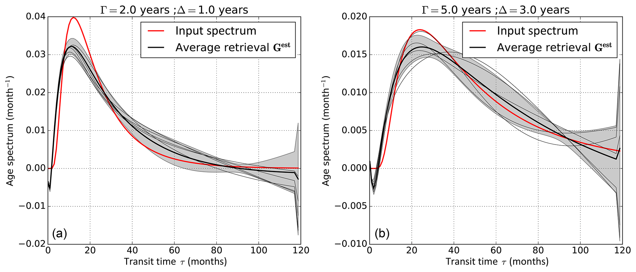
Figure 3Input age spectra (red) and average retrieved age spectra (black), for an input idealized age spectrum with Γ=2 years, Δ=1 year (a) and Γ=5 years, Δ=3 years (b). The average retrieved age spectra are averages of 100 retrievals from 100 sets of pseudo-tracer observations χobs (i.e., 100 different realizations of the noise in Eq. 25). The gray shading corresponds to ± the standard deviation of the hundred retrievals and shows the dispersion-noise-induced uncertainty. The thin gray curves are individual retrievals.
3.2.3 Resolution
To perform the retrieval presented above, only nine tracers were used, whereas there were the 119 components of the spectrum to invert (monthly bins on a 10-year-long transit time axis). It then comes without surprise that the retrieval is strongly under-constrained and requires regularization, especially since the weighting functions all peak at τ=0. The effective resolution in transit time of the inverted spectrum can be investigated from the averaging kernel matrix A defined by Eq. (23) as
The matrix A quantifies the contribution of the value of G at different transit times to the retrieved age spectrum Gest at a specific transit time, and thus the resolution and ability to distinguish specific features. Averaging kernels peaking at one single transit time would provide the best resolution.
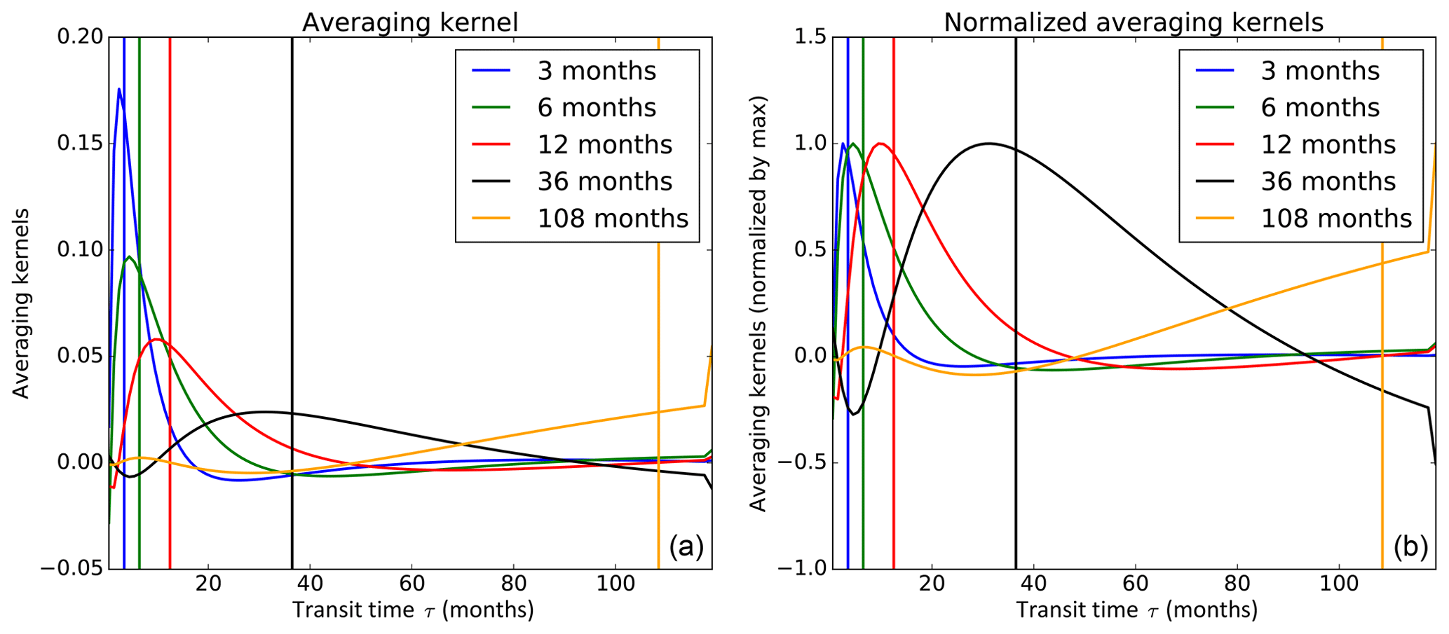
Figure 4Averaging kernels to the age spectrum for different retrieved transit times with the high-resolution (1 month) retrieval. (a) Actual averaging kernels. (b) Averaging kernels normalized by their respective maximum value. Note that the averaging kernel at a particular transit time is the respective row of the averaging kernel matrix.
For our setup, the averaging kernels are displayed in Fig. 4. As expected from the shape of the weighting function (Fig. 1), the resolution is better for short transit times, although even for those the effective resolution does not reach the 1-month-transit-time bin size chosen for the retrieval, as can be seen from the overlap of the averaging kernels. The averaging kernels also exhibit negative lobes, which are responsible for the negative values seen in the retrieval at transit times characterized by low values of G. The amplitude of the negative values may be decreased by strengthening the regularization, but this reduces the sharpness of the peak of the averaging kernels and hence degrades the resolution.
Given the redundancy visible in the averaging kernels, it is possible to use a sparser-resolution grid in transit time, which would better reflect the information available from the tracers. Although there is some freedom in the choice of the grid, we keep the linear grid spacing in the following because of its simplicity and the demonstrated feasibility of the retrievals in that setup.
3.2.4 Tail correction and renormalization
As emphasized above, there is no guarantee that the retrieved age spectrum is positive for all transit times. Although negative values should not be discarded in averaging procedures, some practical applications (such as using the retrieved age spectrum to, for example, compute mean age or estimate the mixing ratio of any tracer) may impose that the retrieved spectrum fulfills the requirements of distribution functions, i.e., to have only positive values and integrate to unity. Renormalization is necessary to enforce those requirements. We propose a simple three-step procedure to obtain a normalized spectrum Gnorm from Gest.
-
Set all negative values to 0.
-
Fit the tail of the age spectrum to an exponential, as was suggested by Li et al. (2012) and employed by Diallo et al. (2012) and Ploeger and Birner (2016). By default, we apply the tail fitting to all transit times larger than half the maximum retrieved transit time; if the fit leads to a positive exponential parameter (exponential growth instead of decay), then a second attempt for a fit is made for transit times from the resolved modal transit time to the end of the transit time axis. If this again leads to an exponential growth, the normalization is considered to have failed and only Step 1 is carried out.
-
Normalize the whole spectrum (including the tail) so that it integrates to 1. In other words, we ensure that
tn is the maximum transit time considered; it is arbitrarily set to 100 years in our case; the only requirement is that tn should be sufficiently large to cover all significantly non-zero values of G. This step is only performed if Step 2 was successful.
4.1 Application to model data
A first application of the inversion method is to retrieve age spectra from tracers in model simulations. To demonstrate this, we use a transport simulation performed with the 3-D version of the Chemical Lagrangian Model of the Stratosphere (CLaMS; McKenna et al., 2002; Konopka et al., 2004). The general setup of the model is described by Pommrich et al. (2014). The model simulation was started on 1 January 1979 and includes a pulse tracer set to estimate the age spectrum using the BIR method similar to the one used by Ploeger and Birner (2016). From the pulse tracer mixing ratios the true model age spectra have been calculated independently using the BIR method, to validate the new age spectrum retrieval. In addition to the pulse tracers, 28 artificial radioactive tracers with boundary conditions at the surface and linear decay rate in the free atmosphere have been introduced. They consist in one tracer with a decay time of 15 days, 17 with decay times ranging from 30 to 510 days with a 30-day step, and 10 with decay times from 570 to 1380 days with a 90-day step. In Fig. 5, the age spectra retrieved from these exponentially decaying tracers using the new method introduced in Sect. 3 are compared to age spectra estimated with the BIR method (Ploeger and Birner, 2016) for different altitude–latitude ranges on 31 December 1983.

Figure 5Age spectra retrieved from artificial decaying radioactive tracers, with (blue) and without (black) renormalization, versus spectra estimated using the BIR method (red). The spectra on the different panels correspond to the same CLaMS model simulation on 31 December 1983, in different altitude–latitude regions (equatorial upper troposphere a, equatorial lower stratosphere b, equatorial middle stratosphere c, midlatitude middle stratosphere d). The resolution along the transit time axis is 1 month (the transit times retrieved a span of 0 to 4 years) and the chosen regularization strength is .
Figure 5 illustrates the unequal performance of the inversion in the different cases. For short transit times, seen in the tropical upper troposphere (Fig. 5a), the shape of the age spectrum is very well captured, despite the sharpness of the modal peak. At higher altitudes in the tropical pipe (Fig. 5b), the transit time distribution exhibits two peaks, with the first mode corresponding to the (most recent) “direct ascension” from the surface while the second is a remainder from the increased entry of air in the stratosphere during the previous winter compared to the subsequent spring (see Ploeger and Birner, 2016, for further discussion of age spectrum seasonality). This bimodal behavior is smoothed out in the retrieval so that the two modes cannot be distinguished from one another in the retrieved spectrum, but the tail and general shape of the spectrum are well represented. Only the mode from the previous winter has reached higher up (Fig. 5c), which results in a translated spectrum with a larger tail compared to the ones displayed in panels (a) and (b). The full magnitude of the main peak is not reproduced in the retrieval, although its location is correct. The multipeak structure resulting from the seasonal cycle in the Northern Hemisphere stratosphere is completely smoothed out (Fig. 5d).
The different examples above show that the (radioactively) decaying-tracer setup effectively enables the retrieval of the general shape of the age spectrum. However, high-resolution features, such as the magnitude of individual peaks or the seasonal cycle in the age spectrum, are either underestimated or not retrieved at all, in particular fine-scale structures at large transit times. The comparison of the quality of the retrievals for different input spectra in panels (a) and (c) emphasizes the better resolution for short transit times. This is an immediate consequence of the shape of the averaging kernels, which are wider for large transit times (Fig. 4), due to the shape of the weighting functions for the radioactive tracers (Fig. 1).
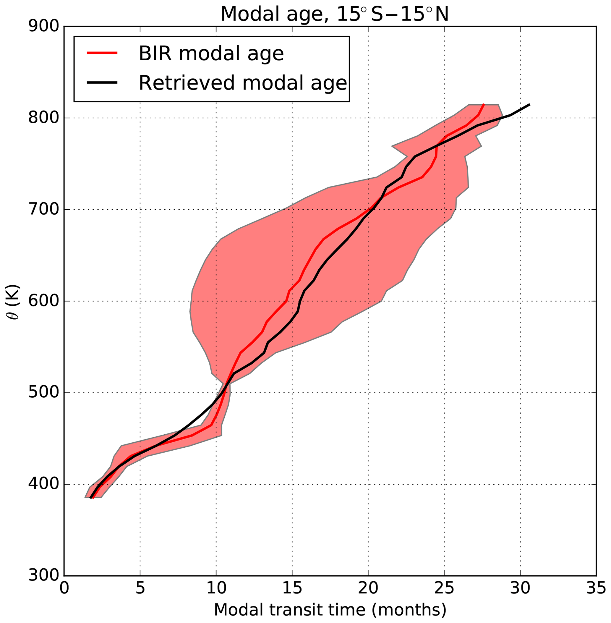
Figure 6Profile of tropical (15∘ S–15∘ N) modal age on 31 December 1983 in the CLaMS simulation, determined using the BIR method (red) or retrieved using the procedure highlighted in Sect. 3 (black). The red shading corresponds to ± the standard deviation of the mode of the BIR spectrum in the 15∘ S–15∘ N region and is introduced to guide the eye regarding the range of variability.
The better quality of the retrievals for short transit times makes them most useful in the “ventilated” regions, i.e., the tropical pipe and the midlatitude surf zone. This is illustrated in Fig. 6, which contrasts the actual modal age of air determined with the BIR method with that derived using the retrieval procedure within the tropical pipe. As shown by Ploeger and Birner (2016), in the tropical pipe (as well as in the wintertime stratospheric surf zone) the modal age is a useful indicator of the residual circulation transit time. Figure 6 shows that the retrieved tropical modal age agrees reasonably well with the BIR modal age (consistent with Fig. 5a, b). This is also the case for the young-age spectra of the midlatitude lower stratosphere (Fig. 5c).
Thanks to the sensitivity of the retrievals to young ages, the normalized retrieved spectra can provide a realistic view of the content in young air masses (younger than a few months) and its variability. The mass fraction of air younger than 6 months (F6) from the retrieval method is compared to the respective fraction from the pulse method in Fig. 7, exemplarily for 31 December 1983. In the lower stratosphere (here 400 K), the young air mass fractions from both methods agree very well, even for details such as the regions of youngest air above the Indian Ocean and west Pacific or the wavelike structures in the subtropics. Hence, the retrieval method can be used to infer quantitative characteristics on rapid transport in the upper troposphere–lower stratosphere. However, for age spectra with long tails towards large transit times and a number of distinct peaks corresponding to the seasonal cycle, such as encountered in the midlatitude polar mid-stratosphere (Fig. 5d), large errors occur. These errors partly originate from the coarser description of the spectrum at large transit times and partly from the inability of the inversion to capture the annual cycle. Introducing other tracers in the retrieval might allow improvement on this aspect, as investigated in the following section.
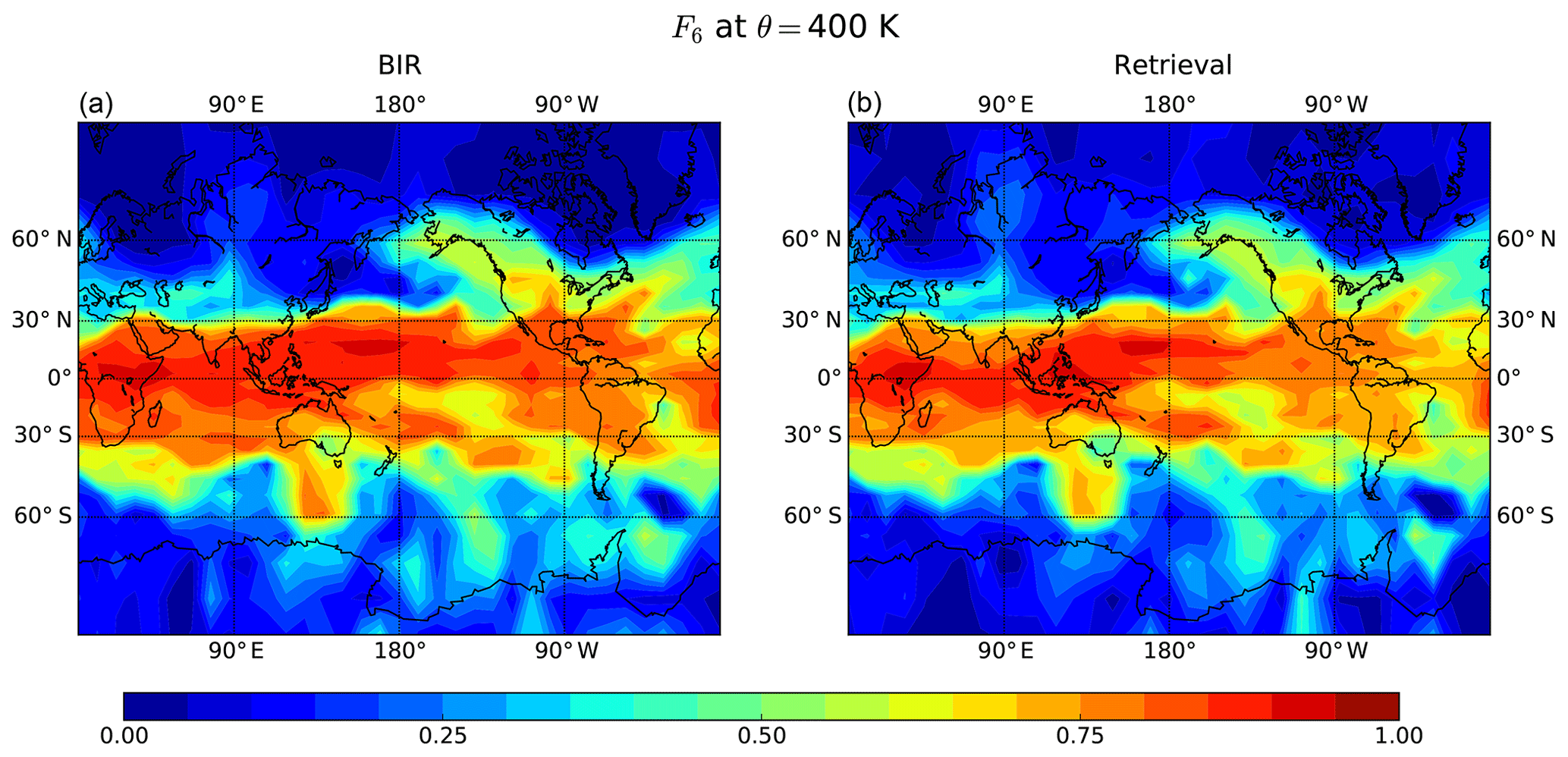
Figure 7Young (τ<6 months) air mass fraction F6 at θ=400 K on 31 December 1983, as estimated from the BIR method (a) and the retrieval (b).
4.2 Use of additional tracers to retrieve realistic age spectra
In addition to parent radioactive tracers, Eq. (8) also encompasses daughter radioactive tracers, which are for instance the products of the decay of a surface emitted tracer, following the decay chain:
The rate of change of the mixing ratio ξB of the daughter tracer is given by
Let us now consider a set of parent and daughter tracers, with ξA and ξB the vectors of their mixing ratios. If the boundary condition at the surface for the parent tracers is and for the daughter tracers , and if the decay times are equal for each couple (), then for each k the daughter tracer mixing ratio is given by the following relation:
The weighting functions of transit times, as shown in Fig. 8, peak at different times corresponding to 1∕λk and hence allow a better resolution of the age spectrum. However, they still have the disadvantage of an increasing width of the weighting functions for increasing transit time of the peak. The line of the transfer matrix L corresponding to the lth daughter tracer (i.e., such that ) is
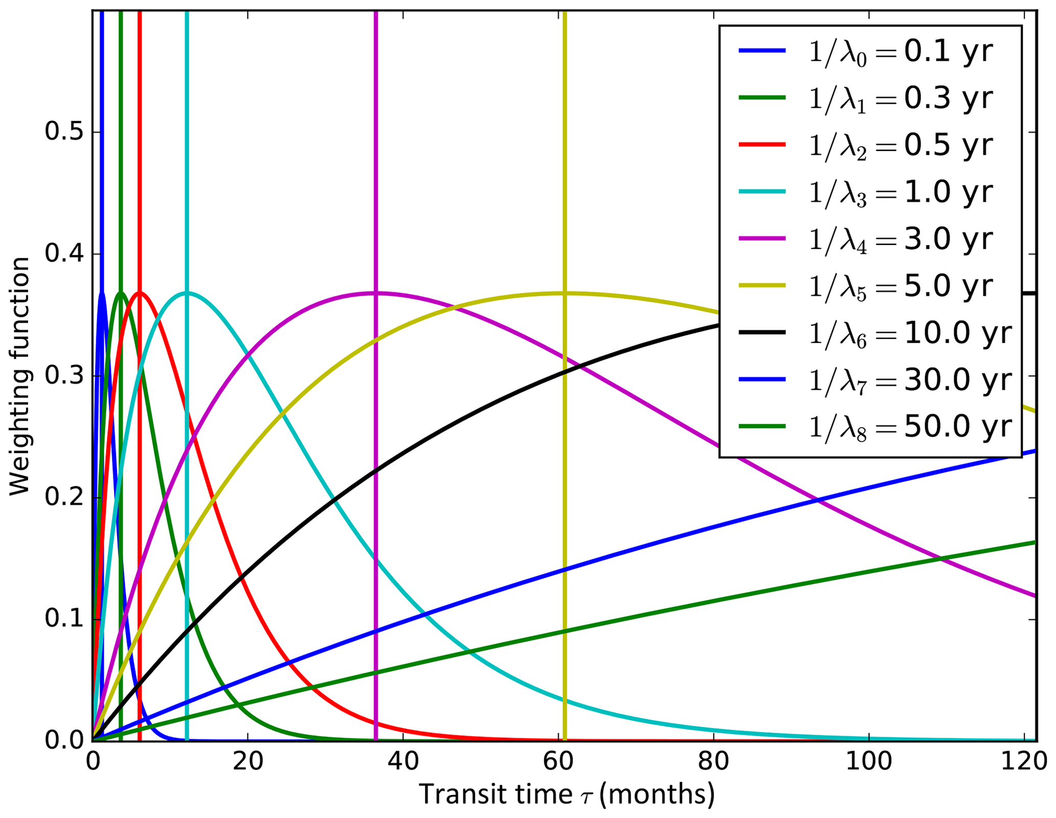
Figure 8Shape of the weighting function to the age spectrum for radioactive or chemical product tracers with lifetimes 1∕λk equal to that of the parent species. The vertical lines show the location of the maxima of the weighting functions, reached at transit times .
We added a set of such daughter tracers to the parent radioactive tracers used in Sect. 3.2. The method employed to initialize the tracers and set up the retrievals is the same as the one presented in Sect. 3.2, except that the basic spectrum is now given by
where ω=2π yr−1 is the angular frequency, A the amplitude and ϕ the phase of the annual cycle, and is a normalization constant. This functional form, introduced by Hauck et al. (2018), is an adjustment of Eq. (24) allowing the inclusion of the seasonal cycle. Note that with this form, Γ and Δ now slightly differ from the mean age and the age spectrum width.
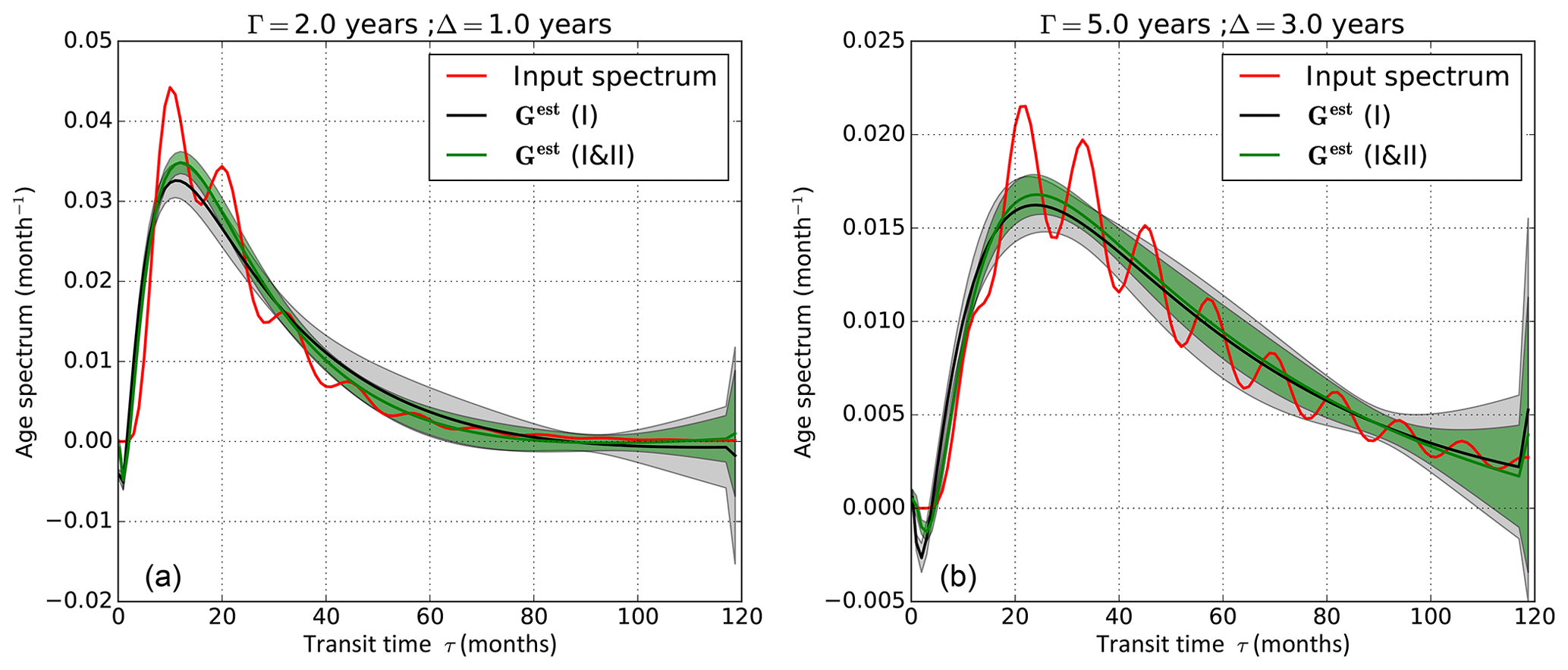
Figure 9Input age spectra (red), defined using Eq. (33) with A=0.3, (for left and right panels), Γ=2 years and Δ=1 year (a) and Γ=5 years, Δ=3 years (b). Retrieved age spectra using (black) parent decaying tracers only or (green) both parent and daughter tracers. The full lines are average retrieved age spectra over 100 retrievals from 100 sets of pseudo-tracer observations. The gray and green shadings correspond to ± the standard deviation of the 100 retrievals and show the dispersion-noise-induced uncertainty.
Figure 9 shows the results of the retrieval experiment. The input spectra (red curves) bear resemblance with the realistic spectra in Fig. 5c, d. In particular, they exhibit a clear annual cycle, evident from the annually repeating peaks. The default retrieval using only parent tracers (black curves) does not fit this pattern and has essentially the same shape as for an input without seasonal variability (as in Fig. 3). With both parent and daughter tracers (green curves), the fit to the input spectrum is improved. In particular, the uncertainty is clearly reduced. However, the seasonal variability is still absent from the retrieval.
To retrieve the seasonal variability in the age spectrum, we include another type of tracers. These are pairs of conserved tracers subject to periodic boundary conditions, such as sinusoidal tracers varying as
where ωm is the angular frequency of the oscillations. Such a pair of tracers in phase quadrature will provide additional information on periodic variations in the spectrum, like the seasonal cycle. The transfer matrix coefficients for those tracers are (calculated from Eq. 17)

Figure 10Input age spectra (red), defined using Eq. (33) with A=0.3, (for left and right panels), Γ=2 years and Δ=1 year (a) and Γ=5 years, Δ=3 years (b). Retrieved age spectra using (black) parent decaying tracers only or (green) daughter and parent tracers and two sets of periodic tracers with periods of 1 and 2 years. The full lines are average retrieved age spectra over 100 retrievals from 100 sets of pseudo-tracer observations. The gray and green shadings correspond to ± the standard deviation of the 100 retrievals and show the dispersion-noise-induced uncertainty.
We added a set of sinusoidal tracers with periods of 1 and 2 years in addition to the set of parent radioactive tracers used in Sect. 3.2 and the daughter tracers discussed above to further improve the retrieval. The retrieval results are shown in Fig. 10. The addition of the periodic tracers (red curve) enables us to retrieve the seasonality in the spectrum without deteriorating the representation of the general shape of the spectrum. Hence, it appears that with an adequate pool of time-varying tracers, high-frequency features in the spectrum, such as the seasonal cycle, can be retrieved.
4.3 Application to observable tracers
Although it is beyond the scope of our study to retrieve atmospheric age spectra from actual tracer measurements, a few further points should be mentioned regarding the practical applicability of our method. First, a major limitation resides in the uncertainties associated with the forward model (Eqs. 7 and 8) for chemically active tracers, in particular regarding the constant-lifetime assumption. Indeed, in the real atmosphere, the actual path taken by the fluid element strongly influences the lifetime of the species (through changes in the photochemical exposure for instance). Schoeberl et al. (2000, 2005) have argued that the path-dependent lifetime may be reduced to a position-dependent average lifetime, but the validity of this approximation remains to be assessed. The difficulty of having a variable lifetime may also be partly circumvented by including age-dependent decay rates λ(τ). This nevertheless assumes that the path dependence of the lifetime may be condensed in the age information and depends on an estimation of the lifetime as a function of age. Application of the method to chemically active tracers will hence require a careful examination of their lifetime variability, which can only be determined using chemistry–transport models.
The practical feasibility of our methodology is more obvious in the case of inert-tracer measurements for which Eq. (7) also holds (with λ=0), as stated already in Sect. 2.2.1. For those, we expect that it can be applied straightforwardly to in situ or remote-sensing measurements, as long as
-
the time-dependent boundary condition (and its spatial variability) are known and
-
the different sources of errors (uncertainties in the boundary conditions and the measurements themselves) are appropriately considered and included in the definition of the error covariance matrix Sϵ (Eq. 23).
Tests with idealized distributions, as shown in Sect. 3.2, enable us to find out which properties of the transit time distribution can be inferred from a given set of tracers. The experiments presented above already provide some general insight into this problem.
In general, our experiments show that short-lived species with exponential decay or conserved tracers increasing exponentially at the surface can provide detailed information on the transit time distribution for rapid transport, as suggested by Fig. 5. They might be sufficient to retrieve the age spectrum in the free troposphere resulting from convective transport from the boundary layer. For the stratosphere, with longer transport timescales involved and delayed arrivals of air masses, the parent radioactive tracers still carry some information on the transit time distribution, but their usefulness is more limited. In particular, they alone cannot be used to retrieve the annual cycle in age of air. However, they might be combined with long-lived tracers that exhibit an annual cycle (such as CO2) to better constrain the age spectrum. The potential of the method in practical use will depend on the measured tracer set and can be estimated following the steps outlined in Sect. 3.
The concentrations in chemical tracers with different dependencies on transit time carry information on the age of air spectrum, the transit time distribution from the surface to a given location in the atmosphere. In this paper, we propose a method to retrieve the age of air spectrum from different trace gas species' mixing ratios. Formulating the question as an inverse problem, its dimension and complexity are by far more manageable than those of the inversions routinely performed for satellite retrievals of temperature and tracer profiles. In particular, the forward model (a mere convolution) is linear and, depending on the tracer considered, the uncertainties can be fairly well known compared to those of radiative transfer 3. A simple Tikhonov regularization appears sufficient to constrain the problem and retrieve the atmospheric transit time distribution.
Using prescribed age of air spectra and a set of artificial decaying radioactive tracers, we demonstrated the feasibility of the approach: even in the presence of forward model uncertainties and noise, the retrieved distributions are in reasonable agreement with the input age spectra. Furthermore, we applied the method to atmospheric transport simulations with the reanalysis-driven CLaMS model; the age spectra retrieved from a set of parent decaying tracers compared relatively well with spectra derived using the boundary impulse response method, especially regarding the general shape of the distribution. However, fine-scale features, such as the seasonal cycle in transit-time frequency, could not be captured with only-decaying tracers due to the large width of the averaging kernels. We show that the caveat may be circumvented by including trace gas species with seasonally varying concentrations at the surface and daughter decaying species in the retrieval.
The methodology introduced in this work can be applied in a number of situations. First, it might prove useful for the estimation of age spectra in models. Indeed, the most commonly used method, the boundary impulse response method (Li et al., 2012; Ploeger and Birner, 2016), requires an increasing number of tracers with increasing maximum resolved transit time, which is cumbersome and computationally expensive, especially in Eulerian models (Li et al., 2012). It has, in particular, the disadvantage of a constant resolution as a function of transit time, which leads to unnecessarily high resolution to describe the tail at long transit times. With a refined set of artificial tracers (combining pulse and non-pulse tracers), the inversion approach may enable an accurate and resolved description of the age spectrum at a reasonable computational cost.
However, the age spectrum retrieval approach might be most useful when trying to estimate transit time distributions from observations. An important number of tracers with different lifetimes and surface tendencies can today be measured by AirCore suspended from balloons (Membrive et al., 2017; Engel et al., 2017) and whole air samplers onboard aircraft (as was carried out in some recent campaigns; e.g., Pan et al., 2017; Jensen et al., 2017). Although more limited in resolution, some remote-sensing instruments, such as GLORIA (Riese et al., 2014), MIPAS (Stiller et al., 2012; Kellmann et al., 2012; Haenel et al., 2015) or ACE-FTS (Bernath et al., 2005), can also retrieve an important number of relevant atmospheric species to which this approach could be applied. We hope that our methodology will pave the way for a more precise and global characterization of transit time spectra from observations in the future.
This research does not rely directly on any data. The CLaMS model outputs can be obtained from the first author upon request.
Here, we illustrate the ill-posed nature of the direct inversion of the age spectrum from tracer concentrations. This approach is written as (Schoeberl et al., 2000)
We use a similar setup as in Sect. 3, except that the number of transit time bins is now equal to the number of radioactive tracers with distinct decay times. The matrix L is then square and can be directly inverted, as suggested by Schoeberl et al. (2000). The spectrum estimated using that approach is shown in Fig. A1. It exhibits large oscillations associated with the ill-posed, underconstrained problem. These oscillations are also present for a regression (Eq. 23 with α2=0) without the regularization terms (not shown), demonstrating the necessity of the regularization.
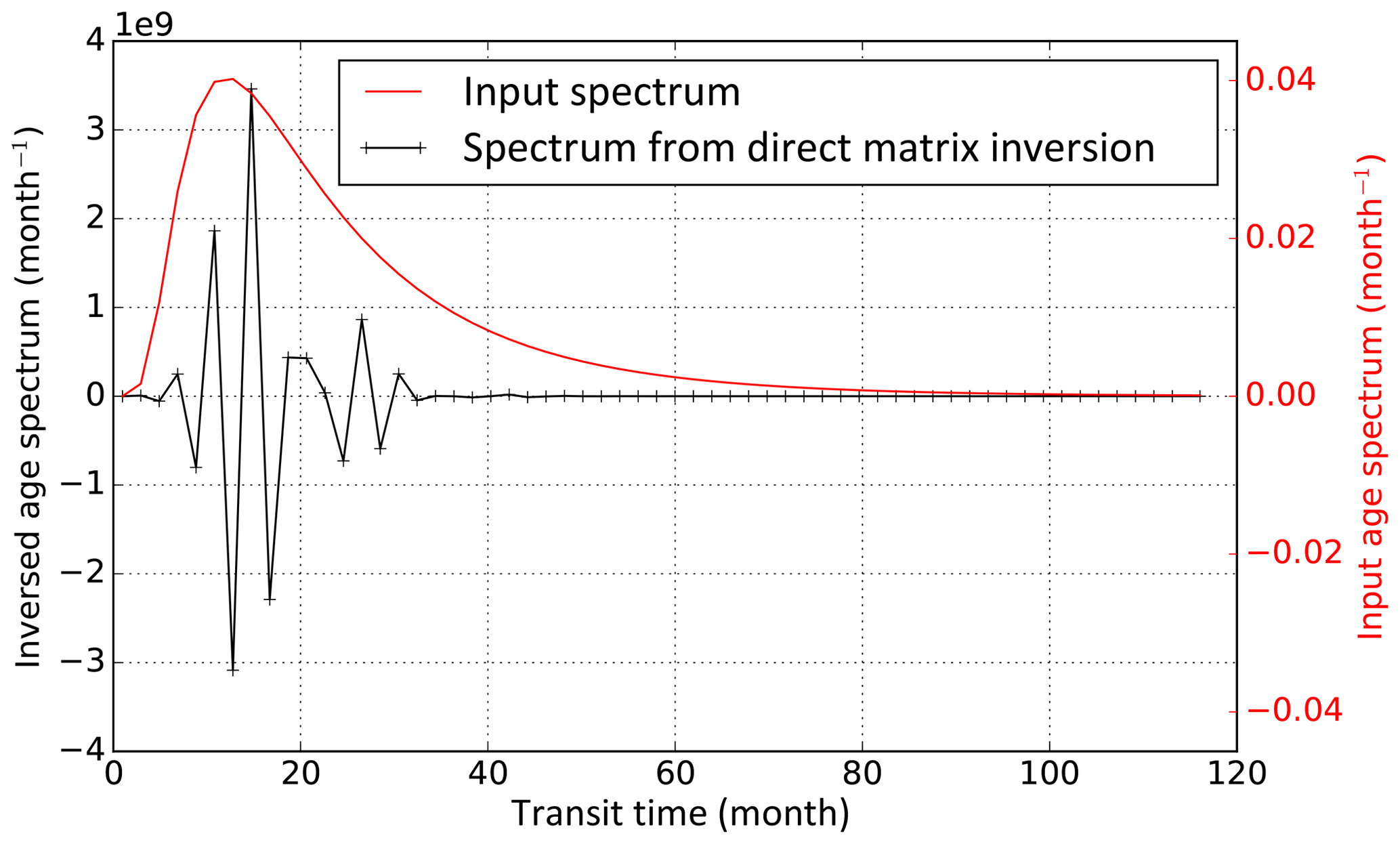
Figure A1Age spectrum from a direct inversion (Eq. A1) using a set of radioactive tracers (black) vs. input age spectrum (red). Note that due to the huge amplitude of the characteristic oscillations associated with the ill-posed, underconstrained problem, different y axes are used for the inversed and input age spectra.
AP had the original idea and designed the study with suggestions from FP. AP performed the CLaMS simulations using the age spectrum and BIR tracer setup implemented by FP. AP carried out the analysis and wrote the paper, with contributions from FP.
The authors declare that they have no conflict of interest.
The authors thank Lukas Krasauskas, Isabell Krisch and Jörn Ungermann for their advice regarding the inversion methodology
and Marius Hauck, Frauke Fritsch and Hella Garny for useful discussions. We are especially grateful to Lukas Krasauskas for his
comments on an earlier version of the paper. Insightful comments by the two anonymous referees are gratefully acknowledged.
This study was funded by the Helmholtz Association under grant VH-NG-1128 (Helmholtz Young Investigators Group A–SPECi).
The article processing charges for this open-access
publication were covered by a Research
Centre of the Helmholtz Association.
Edited by: Federico Fierli
Reviewed by: two anonymous referees
Andrews, A. E., Boering, K. A., Daube, B. C., Wofsy, S. C., Hintsa, E. J., Weinstock, E. M., and Bui, T. P.: Empirical age spectra for the lower tropical stratosphere from in situ observations of CO2: Implications for stratospheric transport, J. Geophys. Res.-Atmos., 104, 26581–26595, https://doi.org/10.1029/1999JD900150, 1999. a, b
Bernath, P. F., McElroy, C. T., Abrams, M. C., Boone, C. D., Butler, M., Camy-Peyret, C., Carleer, M., Clerbaux, C., Coheur, P.-F., Colin, R., DeCola, P., DeMazière, M., Drummond, J. R., Dufour, D., Evans, W. F. J., Fast, H., Fussen, D., Gilbert, K., Jennings, D. E., Llewellyn, E. J., Lowe, R. P., Mahieu, E., McConnell, J. C., McHugh, M., McLeod, S. D., Michaud, R., Midwinter, C., Nassar, R., Nichitiu, F., Nowlan, C., Rinsland, C. P., Rochon, Y. J., Rowlands, N., Semeniuk, K., Simon, P., Skelton, R., Sloan, J. J., Soucy, M.-A., Strong, K., Tremblay, P., Turnbull, D., Walker, K. A., Walkty, I., Wardle, D. A., Wehrle, V., Zander, R., and Zou, J.: Atmospheric Chemistry Experiment (ACE) Mission overview, Geophys. Res. Lett., 32, L15S01, https://doi.org/10.1029/2005GL022386, 2005. a
Butchart, N., Cionni, I., Eyring, V., Shepherd, T. G., Waugh, D. W., Akiyoshi, H., Austin, J., Brühl, C., Chipperfield, M. P., Cordero, E., Dameris, M., Deckert, R., Dhomse, S., Frith, S. M., Garcia, R. R., Gettelman, A., Giorgetta, M. A., Kinnison, D. E., Li, F., Mancini, E., McLandress, C., Pawson, S., Pitari, G., Plummer, D. A., Rozanov, E., Sassi, F., Scinocca, J. F., Shibata, K., Steil, B., and Tian, W.: Chemistry–Climate Model Simulations of Twenty-First Century Stratospheric Climate and Circulation Changes, J. Climate, 23, 5349–5374, https://doi.org/10.1175/2010JCLI3404.1, 2010. a
Diallo, M., Legras, B., and Chédin, A.: Age of stratospheric air in the ERA-Interim, Atmos. Chem. Phys., 12, 12133–12154, https://doi.org/10.5194/acp-12-12133-2012, 2012. a, b, c
Engel, A., Möbius, T., Bönisch, H., Schmidt, U., Heinz, R., Levin, I., Atlas, E., Aoki, S., Nakazawa, T., Sugawara, S., Moore, F., Hurst, D., Elkins, J., Schauffler, S., Andrews, A., and Boering, K.: Age of stratospheric air unchanged within uncertainties over the past 30 years, Nat. Geosci., 2, 28–31, https://doi.org/10.1038/ngeo388, 2009. a, b
Engel, A., Bönisch, H., Ullrich, M., Sitals, R., Membrive, O., Danis, F., and Crevoisier, C.: Mean age of stratospheric air derived from AirCore observations, Atmos. Chem. Phys., 17, 6825–6838, https://doi.org/10.5194/acp-17-6825-2017, 2017. a
Haenel, F. J., Stiller, G. P., von Clarmann, T., Funke, B., Eckert, E., Glatthor, N., Grabowski, U., Kellmann, S., Kiefer, M., Linden, A., and Reddmann, T.: Reassessment of MIPAS age of air trends and variability, Atmos. Chem. Phys., 15, 13161–13176, https://doi.org/10.5194/acp-15-13161-2015, 2015. a, b
Hall, T. M. and Plumb, A. R.: Age as a diagnostic of stratospheric transport, J. Geophys. Res., 99, 1059–1070, https://doi.org/10.1029/93JD03192, 1994. a, b, c
Hall, T. M., Haine, T. W. N., and Waugh, D. W.: Inferring the concentration of anthropogenic carbon in the ocean from tracers, Global Biogeochem. Cy., 16, 78-1–78-15, https://doi.org/10.1029/2001GB001835, 2002. a, b
Hansen, P.: Analysis of Discrete Ill-Posed Problems by Means of the L-Curve, SIAM Rev., 34, 561–580, https://doi.org/10.1137/1034115, 1992. a
Hauck, M., Fritsch, F., Garny, H., and Engel, A.: Deriving stratospheric age of air spectra using chemically active trace gases, Atmos. Chem. Phys. Discuss., https://doi.org/10.5194/acp-2018-991, in review, 2018. a, b
Holzer, M. and Hall, T. M.: Transit-Time and Tracer-Age Distributions in Geophysical Flows, J. Atmos. Sci., 57, 3539–3558, https://doi.org/10.1175/1520-0469(2000)057<3539:TTATAD>2.0.CO;2, 2000. a
Holzer, M., McKendry, I. G., and Jaffe, D. A.: Springtime trans-Pacific atmospheric transport from east Asia: A transit-time probability density function approach, J. Geophys. Res.-Atmos., 108, 4708, https://doi.org/10.1029/2003JD003558, 2003. a
Jensen, E. J., Pfister, L., Jordan, D. E., Bui, T. V., Ueyama, R., Singh, H. B., Thornberry, T. D., Rollins, A. W., Gao, R.-S., Fahey, D. W., Rosenlof, K. H., Elkins, J. W., Diskin, G. S., DiGangi, J. P., Lawson, R. P., Woods, S., Atlas, E. L., Rodriguez, M. A. N., Wofsy, S. C., Pittman, J., Bardeen, C. G., Toon, O. B., Kindel, B. C., Newman, P. A., McGill, M. J., Hlavka, D. L., Lait, L. R., Schoeberl, M. R., Bergman, J. W., Selkirk, H. B., Alexander, M. J., Kim, J.-E., Lim, B. H., Stutz, J., and Pfeilsticker, K.: The NASA Airborne Tropical Tropopause Experiment: High-Altitude Aircraft Measurements in the Tropical Western Pacific, B. Am. Meteorol. Soc., 98, 129–143, https://doi.org/10.1175/BAMS-D-14-00263.1, 2017. a
Johnson, D. G., Jucks, K. W., Traub, W. A., Chance, K. V., Toon, G. C., Russell, J. M., and McCormick, M. P.: Stratospheric age spectra derived from observations of water vapor and methane, J. Geophys. Res.-Atmos., 104, 21595–21602, https://doi.org/10.1029/1999JD900363, 1999. a, b
Kellmann, S., von Clarmann, T., Stiller, G. P., Eckert, E., Glatthor, N., Höpfner, M., Kiefer, M., Orphal, J., Funke, B., Grabowski, U., Linden, A., Dutton, G. S., and Elkins, J. W.: Global CFC-11 (CCl3F) and CFC-12 (CCl2F2) measurements with the Michelson Interferometer for Passive Atmospheric Sounding (MIPAS): retrieval, climatologies and trends, Atmos. Chem. Phys., 12, 11857–11875, https://doi.org/10.5194/acp-12-11857-2012, 2012. a
Konopka, P., Steinhorst, H.-M., Grooß, J.-U., Günther, G., Müller, R., Elkins, J. W., Jost, H.-J., Richard, E., Schmidt, U., Toon, G., and McKenna, D. S.: Mixing and ozone loss in the 1999–2000 Arctic vortex: Simulations with the three-dimensional Chemical Lagrangian Model of the Stratosphere (CLaMS), J. Geophys. Res.-Atmos., 109, D02315, https://doi.org/10.1029/2003JD003792, 2004. a
Li, F., Waugh, D. W., Douglass, A. R., Newman, P. A., Pawson, S., Stolarski, R. S., Strahan, S. E., and Nielsen, J. E.: Seasonal variations of stratospheric age spectra in the Goddard Earth Observing System Chemistry Climate Model (GEOSCCM), J. Geophys. Res.-Atmos., 117, D05134, https://doi.org/10.1029/2011JD016877, 2012. a, b, c, d, e, f, g
McKenna, D. S., Konopka, P., Grooß, J.-U., Günther, G., Müller, R., Spang, R., Offermann, D., and Orsolini, Y.: A new Chemical Lagrangian Model of the Stratosphere (CLaMS) 1. Formulation of advection and mixing, J. Geophys. Res.-Atmos., 107, ACH 15-1–ACH 15-15, https://doi.org/10.1029/2000JD000114, 2002. a
Membrive, O., Crevoisier, C., Sweeney, C., Danis, F., Hertzog, A., Engel, A., Bönisch, H., and Picon, L.: AirCore-HR: a high-resolution column sampling to enhance the vertical description of CH4 and CO2, Atmos. Meas. Tech., 10, 2163–2181, https://doi.org/10.5194/amt-10-2163-2017, 2017. a
Orbe, C., Waugh, D. W., Newman, P. A., and Steenrod, S.: The Transit-Time Distribution from the Northern Hemisphere Midlatitude Surface, J. Atmos. Sci., 73, 3785–3802, 2016. a
Pan, L. L., Atlas, E. L., Salawitch, R. J., Honomichl, S. B., Bresch, J. F., Randel, W. J., Apel, E. C., Hornbrook, R. S., Weinheimer, A. J., Anderson, D. C., Andrews, S. J., Baidar, S., Beaton, S. P., Campos, T. L., Carpenter, L. J., Chen, D., Dix, B., Donets, V., Hall, S. R., Hanisco, T. F., Homeyer, C. R., Huey, L. G., Jensen, J. B., Kaser, L., Kinnison, D. E., Koenig, T. K., Lamarque, J.-F., Liu, C., Luo, J., Luo, Z. J., Montzka, D. D., Nicely, J. M., Pierce, R. B., Riemer, D. D., Robinson, T., Romashkin, P., Saiz-Lopez, A., Schauffler, S., Shieh, O., Stell, M. H., Ullmann, K., Vaughan, G., Volkamer, R., and Wolfe, G.: The Convective Transport of Active Species in the Tropics (CONTRAST) Experiment, B. Am. Meteorol. Soc., 98, 106–128, https://doi.org/10.1175/BAMS-D-14-00272.1, 2017. a
Ploeger, F. and Birner, T.: Seasonal and inter-annual variability of lower stratospheric age of air spectra, Atmos. Chem. Phys., 16, 10195–10213, https://doi.org/10.5194/acp-16-10195-2016, 2016. a, b, c, d, e, f, g, h, i, j
Pommrich, R., Müller, R., Grooß, J.-U., Konopka, P., Ploeger, F., Vogel, B., Tao, M., Hoppe, C. M., Günther, G., Spelten, N., Hoffmann, L., Pumphrey, H.-C., Viciani, S., D'Amato, F., Volk, C. M., Hoor, P., Schlager, H., and Riese, M.: Tropical troposphere to stratosphere transport of carbon monoxide and long-lived trace species in the Chemical Lagrangian Model of the Stratosphere (CLaMS), Geosci. Model Dev., 7, 2895–2916, https://doi.org/10.5194/gmd-7-2895-2014, 2014. a
Ray, E. A., Moore, F. L., Rosenlof, K. H., Davis, S. M., Sweeney, C., Tans, P., Wang, T., Elkins, J. W., Boenisch, H., Engel, A., Sugawara, S., Nakazawa, T., and Aoki, S.: Improving stratospheric transport trend analysis based on SF6 and CO2 measurements, J. Geophys. Res., 119, 14110–14128, 2014. a
Reithmeier, C., Sausen, R., and Grewe, V.: Investigating lower stratospheric model transport: Lagrangian calculations of mean age and age spectra in the GCM ECHAM4, Clim. Dynam., 30, 225–238, https://doi.org/10.1007/s00382-007-0294-1, 2008. a
Riese, M., Ploeger, F., Rap, A., Vogel, B., Konopka, P., Dameris, M., and Forster, P.: Impact of uncertainties in atmospheric mixing on simulated UTLS composition and related radiative effects, J. Geophys. Res.-Atmos., 117, D16305, https://doi.org/10.1029/2012JD017751, 2012. a
Riese, M., Oelhaf, H., Preusse, P., Blank, J., Ern, M., Friedl-Vallon, F., Fischer, H., Guggenmoser, T., Höpfner, M., Hoor, P., Kaufmann, M., Orphal, J., Plöger, F., Spang, R., Suminska-Ebersoldt, O., Ungermann, J., Vogel, B., and Woiwode, W.: Gimballed Limb Observer for Radiance Imaging of the Atmosphere (GLORIA) scientific objectives, Atmos. Meas. Tech., 7, 1915–1928, https://doi.org/10.5194/amt-7-1915-2014, 2014. a
Rodgers, C. D.: Inverse methods for atmospheric sounding: theory and practice, World Scientific Publishing, 2000. a
Schoeberl, M. R., Sparling, L. C., Jackman, C. H., and Fleming, E. L.: A Lagrangian view of stratospheric trace gas distributions, J. Geophys. Res.-Atmos., 105, 1537–1552, https://doi.org/10.1029/1999JD900787, 2000. a, b, c, d, e, f, g, h, i, j
Schoeberl, M. R., Douglass, A. R., Polansky, B., Boone, C., Walker, K. A., and Bernath, P.: Estimation of stratospheric age spectrum from chemical tracers, J. Geophys. Res.-Atmos., 110, D21303, https://doi.org/10.1029/2005JD006125, 2005. a, b, c, d, e
Stiller, G. P., von Clarmann, T., Haenel, F., Funke, B., Glatthor, N., Grabowski, U., Kellmann, S., Kiefer, M., Linden, A., Lossow, S., and López-Puertas, M.: Observed temporal evolution of global mean age of stratospheric air for the 2002 to 2010 period, Atmos. Chem. Phys., 12, 3311–3331, https://doi.org/10.5194/acp-12-3311-2012, 2012. a, b
Ungermann, J., Blank, J., Lotz, J., Leppkes, K., Hoffmann, L., Guggenmoser, T., Kaufmann, M., Preusse, P., Naumann, U., and Riese, M.: A 3-D tomographic retrieval approach with advection compensation for the air-borne limb-imager GLORIA, Atmos. Meas. Tech., 4, 2509–2529, https://doi.org/10.5194/amt-4-2509-2011, 2011. a
Waugh, D. W. and Hall, T. M.: Age of stratospheric air: Theory, observations, and models, Rev. Geophys., 40, 1010, https://doi.org/10.1029/2000RG000101, 2002. a, b, c, d, e
Waugh, D. W., Hall, T. M., and Haine, T. W. N.: Relationships among tracer ages, J. Geophys. Res.-Oceans, 108, https://doi.org/10.1029/2002JC001325, 2003. a, b, c, d
Waugh, D. W., Crotwell, A. M., Dlugokencky, E. J., Dutton, G. S., Elkins, J. W., Hall, B. D., Hintsa, E. J., Hurst, D. F., Montzka, S. A., Mondeel, D. J., Moore, F. L., Nance, J. D., Ray, E. A., Steenrod, S. D., Strahan, S. E., and Sweeney, C.: Tropospheric SF6: Age of air from the Northern Hemisphere midlatitude surface, J. Geophys. Res., 118, 11429–11441, 2013. a
We write “conceptually” because it is clear that physically an air parcel cannot be decomposed into an “infinity of infinitesimal...”. This physical restriction, however, is not a conceptual restriction because at scales considered here this issue has no bearing.
Note that with the normalization of ξk(t) by its time-dependent surface value , Eq. (9) also applies to inert tracers exponentially increasing at the surface with growth rates λk, thus avoiding the constant-lifetime assumption.
This is at least the case for inert tracers; for chemically active tracers the sources of uncertainties are many and more difficult to quantify.
- Abstract
- Introduction
- Theoretical background: relationship between age spectrum and tracers
- Inversion of the age spectrum from (non-pulse) tracers
- Applications and discussion
- Conclusions
- Data availability
- Appendix A: Direct inversion using radioactive tracer concentrations
- Author contributions
- Competing interests
- Acknowledgements
- References