Characterization of transport regimes and the polar dome during Arctic spring and summer using in situ aircraft measurements

The springtime composition of the Arctic lower troposphere is to a large extent controlled by the transport of midlatitude air masses into the Arctic. In contrast, precipitation and natural sources play the most important role during summer. Within the Arctic region sloping isentropes create a barrier to horizontal transport, known as the polar dome. The polar dome varies in space and time and exhibits a strong influence on the transport of air masses from midlatitudes, enhancing transport during winter and inhibiting transport during summer.

We analyzed aircraft-based trace gas measurements in the Arctic from two NETCARE airborne field campaigns (July 2014 and April 2015) with the Alfred Wegener Institute Polar 6 aircraft, covering an area from Spitsbergen to Alaska (134 to 17^∘ W and 68 to 83^∘ N). Using these data we characterized the transport regimes of midlatitude air masses traveling to the high Arctic based on CO and CO₂ measurements as well as kinematic 10 d back trajectories. We found that dynamical isolation of the high Arctic lower troposphere leads to gradients of chemical tracers reflecting different local chemical lifetimes, sources, and sinks. In particular, gradients of CO and CO₂ allowed for a trace-gas-based definition of the polar dome boundary for the two measurement periods, which showed pronounced seasonal differences. Rather than a sharp boundary, we derived a transition zone from both campaigns. In July 2014 the polar dome boundary was at 73.5^∘ N latitude and 299–303.5 K potential temperature. During April 2015 the polar dome boundary was on average located at 66–68.5^∘ N and 283.5–287.5 K. Tracer–tracer scatter plots confirm different air mass properties inside and outside the polar dome in both spring and summer.

Further, we explored the processes controlling the recent transport history of air masses within and outside the polar dome. Air masses within the springtime polar dome mainly experienced diabatic cooling while traveling over cold surfaces. In contrast, air masses in the summertime polar dome were diabatically heated due to insolation. During both seasons air masses outside the polar dome slowly descended into the Arctic lower troposphere from above through radiative cooling. Ascent to the middle and upper troposphere mainly took place outside the Arctic, followed by a northward motion. Air masses inside and outside the polar dome were also distinguished by different chemical compositions of both trace gases and aerosol particles. We found that the fraction of amine-containing particles, originating from Arctic marine biogenic sources, is enhanced inside the polar dome. In contrast, concentrations of refractory black carbon are highest outside the polar dome, indicating remote pollution sources.

Synoptic-scale weather systems frequently disturb the transport barrier formed by the polar dome and foster exchange between air masses from midlatitudes and polar regions. During the second phase of the NETCARE 2014 measurements a pronounced low-pressure system south of Resolute Bay brought inflow from southern latitudes, which pushed the polar dome northward and significantly affected trace gas mixing ratios in the measurement region. Mean CO mixing ratios increased from 77.9±2.5 to 84.9±4.7 ppbv between these two regimes. At the same time CO₂ mixing ratios significantly decreased from 398.16 ± 1.01 to 393.81 ± 2.25 ppmv. Our results demonstrate the utility of applying a tracer-based diagnostic to determine the polar dome boundary for interpreting observations of atmospheric composition in the context of transport history.

1 Introduction

In recent decades the Arctic has undergone dramatic changes affecting sea ice, snow, permafrost, surface temperature, land, and atmospheric circulation (IPCC, 2013). Rising temperatures, increasing twice as fast as in the rest of the world, have led to a significant retreat of Arctic sea ice (Stroeve et al., 2012; Jeffries et al., 2013). In addition to reduced extent, the thickness of sea ice has continuously decreased (Lindsay and Schweiger, 2015).

Midlatitude emissions in the Northern Hemisphere are still the main source region of atmospheric pollutants in the Arctic (Barrie, 1986; Koch and Hansen, 2005; Stohl, 2006; Sharma et al., 2013; Arnold et al., 2016). Several studies based on either in situ measurements or modeling have reported enhanced pollution throughout the Arctic troposphere that is dominated by northern Eurasian sources in the lower troposphere and midlatitude North America and Asia above (Sharma et al., 2006; Shindell et al., 2008; Fisher et al., 2010; Hirdman et al., 2010; Hecobian et al., 2011; Brock et al., 2011; Schmale et al., 2011; Sodemann et al., 2011; Stohl et al., 2013; Law et al., 2014; Monks et al., 2015; Willis et al., 2018). Roiger et al. (2011) even found Asian pollution in the lowermost stratosphere. However, local emissions in specific regions within the Arctic are already important (Stohl et al., 2013; Law et al., 2014; Schmale et al., 2018) and might gain influence in the near future. Continuing retreat of Arctic sea ice will increase the accessibility of the Arctic, thus leading to a potential increase in emissions from local sources of pollutants like shipping (Eckhardt et al., 2013; Corbett et al., 2010; Melia et al., 2016) and oil and gas extraction (Peters et al., 2011). Resulting atmospheric pollutants, such as aerosol and tropospheric ozone, contribute to Arctic warming (Shindell and Faluvegi, 2009; AMAP, 2015).

Compared to other regions of the Northern Hemisphere, the faster pace of the rising surface and lower tropospheric temperatures in the Arctic is commonly known as Arctic amplification (Holland and Bitz, 2003; Screen and Simmonds, 2010). The interplay between different processes fosters feedback mechanisms that further amplify changes in the environment. The decrease in sea ice reduces the surface albedo and increases latent and sensible heat fluxes into the atmosphere, which in turn results in warmer surface temperatures relative to midlatitudes (Robock, 1983; Hall, 2004; Winton, 2006). Furthermore, Pithan and Mauritsen (2014) reported that temperature feedbacks also play an important role for Arctic amplification. Arctic amplification could further cause important changes in the midlatitude circulation (Cohen et al., 2014; Pithan et al., 2018). Zonal winds might weaken and the Rossby wave amplitude is expected to increase, especially during the fall and winter months (Francis and Vavrus, 2012; Francis et al., 2017). Unusually warm sea surface temperatures and low sea ice concentrations in the Arctic have already caused atmospheric circulation anomalies in winter (Lee et al., 2015). As a result, transport pathways for aerosol and pollution into the Arctic will change due to the changing circulation pattern in association with Arctic amplification.

Transport into the Arctic and especially into the Arctic lower troposphere is possible along different pathways, depending on the source area of air masses and the time of the year (Klonecki, 2003; Stohl, 2006; Law and Stohl, 2007; AMAP, 2015). Stohl (2006) identified three major pathways that significantly contribute to transport from major pollution sources into the Arctic lower troposphere. In the following paragraphs we discuss these pathways in turn.

(1) Rapid low-level transport occurs, followed by an uplift at the Arctic front at the location and time when the Arctic front is located far north. For this transport route uplift and potential precipitation occur mostly north of 70^∘ N, which allows for the significant deposition of aerosol and water-soluble pollutants in the Arctic. Stohl (2006) estimated a transport time of 4 d or less. Significant emissions only from densely populated regions in Europe can be transported into the high Arctic lower troposphere via this route because major emission regions in North America and Asia are located south of the polar front. Note that the Arctic front and the polar front are geographically two distinct features. The Arctic front, which is most well defined during the summer months, is thought to develop due to strong differential heating between the cold Arctic ocean and adjacent ice- and snow-free land (Serreze et al., 2001; Crawford and Serreze, 2015). The Arctic front marks the southern boundary of the cold Arctic air mass that is separated from the less cold polar air mass further south. The polar front, in contrast, is the well-known frontal zone separating warm midlatitude and subtropical air masses from colder polar air masses. It is in general located further south compared to the Arctic front and displaced equatorward in summer and poleward in winter. In this baroclinic region characterized by strong horizontal temperature gradients, cyclones develop from an initial disturbance at the front. During the winter months the Arctic front can extend far south over the continents and can eventually be colocated or merge with the polar front.

(2) The low-level transport of already cold air masses into the polar dome occurs, which is associated with further diabatic cooling during the transport timescale of 10–15 d. This pathway from European and high-latitude Asian sources mainly occurs during winter, since transport over snow-covered regions (e.g., Siberia) is involved. Thus, strongly polluted air masses could be transported into the high Arctic lower troposphere. This transport pathway is negligible during the summer months when the surface in Eurasia is a net source of heat (Klonecki, 2003).

(3) Fast uplift occurs, mainly due to convection or warm conveyor belts in southern midlatitudes, followed by high-altitude transport in northerly directions. Radiative cooling eventually leads to a slow descent into the polar dome area after air masses have arrived in the high Arctic. Being less frequent from Europe, this transport pathway is most prevalent from North America and East Asia. In contrast to the other two transport pathways, scavenging processes can occur during the strong ascent in midlatitudes, which can lead to a significant washout of aerosol and soluble pollutants outside the Arctic.

The high Arctic lower troposphere is in general quite well isolated from the rest of the Arctic due to the very cold air masses located in this region. This region is referred to as the polar dome and is characterized by strong temperature contrasts at or near the surface (Arctic front) and sloping isentropes Θ as a result of radiative cooling in the high Arctic, especially during the winter months without sunlight (Barrie, 1986; Klonecki, 2003; Stohl, 2006). In this study we regard the polar dome as the three-dimensional volume of cold air above the Arctic and the Arctic front as its boundary. For instance, if temperature is regarded on a constant pressure level, the Arctic front would separate cold from even colder air masses and would be located in a region of an increased horizontal temperature gradient. This is then similar to the polar front separating subtropical from midlatitude air masses. Air masses preferably maintain near-constant potential temperatures during transport, since atmospheric circulation can be well described by adiabatic motions in the absence of diabatic processes related to clouds, radiation, and turbulence. The potential temperature is low within the polar dome area, and thus only air masses that have experienced diabatic cooling are able to enter the polar dome through the pathways discussed above (Stohl, 2006). As a consequence, the “Arctic haze” phenomenon is mainly fed by northern Eurasian pollution sources when the Arctic front moves southwards since these air masses can drop to temperatures as cold as those in the high Arctic lower troposphere and thus become part of the polar dome (Carlson, 1981, Rahn, 1981, Raatz, 1985, Iversen, 1984, Barrie, 1986, Brock et al., 1990, Dreiling and Friederich, 1997). Already known for decades, Arctic haze has again gained attention at the beginning of the 21st century, triggered by the role of black carbon (BC) in Arctic climate change (Flanner et al., 2007; Hansen and Nazarenko, 2004; Law and Stohl, 2007; McConnell et al., 2007; Quinn et al., 2008; Shindell and Faluvegi, 2009). Pollution originating from outside the Arctic is transported into the high Arctic lower troposphere during the winter months, and the lack of sunlight allows for a build-up of aerosol particles and gaseous pollutants. When temperatures during the winter months become extremely low near the surface, the Arctic lower troposphere is thermally very stably stratified with surface-based inversions that can persist for several days (Bradley et al., 1992). Turbulent exchange and hence dry deposition are reduced under these conditions. Furthermore, the lower troposphere is extremely dry, preventing scavenging of aerosol and gaseous pollutants by wet deposition. At the springtime peak, Arctic haze is often visible as layers of brownish haze affecting the radiation budget of the Arctic lower troposphere and also contributing to the contamination of the Arctic environment. During the transition to pristine summer conditions Arctic haze declines due to efficient aerosol scavenging in midlatitudes during uplift. Anthropogenic aerosol is further reduced by frequent precipitation of low intensity within the Arctic lower troposphere (Barrie, 1986; Browse et al., 2012; Garrett et al., 2010).

In general, the polar dome boundary, acting as a transport barrier for warmer midlatitude air masses, is variable in time and space. Synoptic disturbances can lead to a shift of the polar dome boundary or perturb the transport barrier and foster exchange with midlatitude air that can alter the composition of the lower Arctic troposphere. A distinct definition of the polar dome boundary location is crucial to understand and quantify effects on atmospheric composition. Although the polar dome has been known for decades, only very few specific definitions of the polar dome boundary have been described in the literature. In early studies of Arctic haze, Carlson (1981) or Raatz (1985) identified the polar front as a transport barrier decoupling the Arctic from the influence of midlatitude air masses. More recent studies used the location of the more northern Arctic front as a marker for the polar dome as a transport barrier (Klonecki, 2003; Stohl, 2006). Jiao and Flanner (2016) used the maximum zonal mean latitudinal gradient of 500 hPa geopotential height in the Northern Hemisphere. One of the drawbacks of the latter approach is the missing definition at lower altitudes.

The polar dome is well isolated from the surrounding troposphere, which leads to long residence times of air masses within the polar dome. Anthropogenic tracers like CO and CO₂ show temporal changes within days to weeks due to changes in emissions and the source strength of these species. Furthermore, the distribution of sources and sinks as well as the efficiency of removal processes for both species is different within the Arctic and at midlatitudes, leading to latitudinal gradients for both species. Given the isolation created by the polar dome, we expect measurable gradients in tracer species across its boundary. In this study we use gradients of CO and CO₂ to derive a tracer-based diagnostic to identify the polar dome boundary location. The basis for this analysis is two airborne field campaigns: NETCARE 2014 in July and NETCARE 2015 in April, covering late spring to summer. Despite focusing on only these specific time periods, this study is the first attempt to define the polar dome boundary based on airborne trace gas gradients. We use our trace-gas-based definition of the polar dome boundary to analyze transport history and atmospheric composition within and outside the polar dome.

2 The NETCARE project

The NETCARE project (Network on Climate and Aerosols: Addressing Key Uncertainties in Remote Canadian Environments; http://www.netcare-project.ca, last access: 2 November 2019) is configured around four research activities addressing key uncertainties in the field of Arctic aerosol research (Abbatt et al., 2019). Within this framework two aircraft-based measurement campaigns were performed in the high Arctic. The main objectives of both campaigns were to study aerosol–cloud interactions as well as to characterize local and remote sources for pollution within the high Arctic lower troposphere in summer 2014 (July) and spring 2015 (April). Figure 1 shows a compilation of flight tracks for the two airborne research activities named NETCARE 2014 and NETCARE 2015.

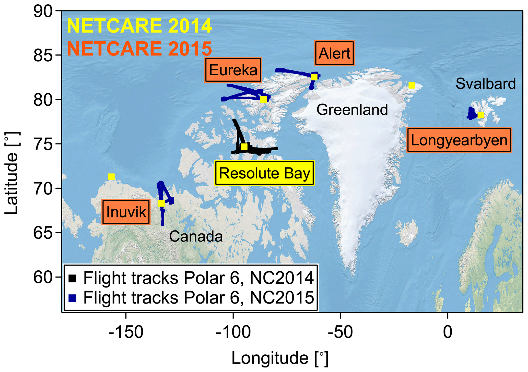
Figure 1 Compilation of research flight tracks during two NETCARE airborne field campaigns in July 2014 and April 2015.

Table 1 Locations and coordinates for the different stations from which measurement flights were performed during the two NETCARE airborne projects in July 2014 and April 2015. Additionally, the time at the station and the number of research flights are given.

The first project was performed from 4 to 21 July 2014 with the Polar 6 aircraft based in Resolute Bay, Nunavut, Canada (e.g., Aliabadi et al., 2016; Leaitch et al., 2016; Willis et al., 2016, 2017; Burkart et al., 2017; Köllner et al., 2017). In total 11 research flights, each 4–6 h long, covered two main areas: Lancaster Sound east of Resolute Bay and north of Resolute Bay where two polynyas (areas of persistent open water) were located. During the last part of the campaign, 19 to 21 July, a special research focus was on ship emission measurements (Aliabadi et al., 2016).

The second aircraft project took place in April 2015. We performed pan-Arctic measurements throughout the European and Canadian Arctic (see Fig. 1). This campaign was a joint NETCARE and PAMARCMiP (Polar Airborne Measurements and Arctic Regional Climate Model Simulation Project; https://www.awi.de/en/focus/sea-ice/in-the-arctic-sea-ices-kindergarten.html, last access: 2 November 2019) project, which will be referred to as “NETCARE 2015” throughout this paper (e.g., Libois et al., 2016; Willis et al., 2019; Schulz et al., 2019). During 10 research flights, each 4–6 h long, we specifically focused on a better understanding of aerosol transport into the Arctic in early spring and its influence on ice cloud formation. More details on the different base stations can be found in Table 1. Multiple vertical profiles from the lowest possible altitude of 60 up to 6000 m were performed to study the vertical distribution of aerosol particles and trace gases.

3 Methodology

3.1 Measurement platform

Airborne measurements were performed using the Polar 6 aircraft of the Alfred Wegener Institute Helmholtz Center for Polar and Marine Research, Bremerhaven, Germany. Polar 6 is a DC 3 aircraft converted to a Basler BT67 (Herber et al., 2008) and modified for operation in cold and harsh environments. The aircraft has a nonpressurized cabin; however, flights up to an altitude of 6 km were regularly performed during the 2014 and 2015 campaigns. The typical survey speed of the aircraft is 120 kts ($\cong \mathrm{60}\mathrm{m}{\mathrm{s}}^{-\mathrm{1}}$) with ascent and descent rates of 150–300 m min⁻¹ during vertical profiles.

3.2 Instrumentation

Meteorological and aircraft altitude data for Polar 6 are provided by the AIMMS-20 instrument. The instrument was designed and manufactured by Aventech Research Inc., Barrie, Ontario, Canada. It includes an air data probe (ADP) that reports the three-dimensional, aircraft-relative flow vector consisting of true air speed, angle of attack, and sideslip. Temperature and relative humidity sensors provide data with an accuracy of 0.30 ^∘C for temperature measurements and 2.0 % for humidity measurements, respectively. A GPS module provided the aircraft 3-D position and inertial velocity. Horizontal and vertical wind speeds were measured with accuracies of 0.50 and 0.75 m s⁻¹, respectively. All data were internally sampled with 200 Hz resolution and for further analysis averaged to 1 Hz resolution. The instrumentation for aerosol and cloud droplets as well as upwelling radiance measurements is described in detail in Leaitch et al. (2016), Willis et al. (2016), Burkart et al. (2017), Aliabadi et al. (2016), Libois et al. (2016), and Schulz et al. (2019).

CO was measured with an Aerolaser ultrafast carbon monoxide (CO) monitor model AL 5002 based on vacuum ultraviolet (VUV) fluorimetry using the excitation of CO at 150 nm. Details on the measurement principle can be found in Gerbig et al. (1999) or Scharffe et al. (2012). The instrument was modified for applying in situ calibrations during in-flight operations. We performed these regular in situ calibrations on a 15 to 30 min time interval during measurement flights using a NIST (National Institute of Standards and Technology) traceable calibration gas with a known CO concentration at atmospheric levels as well as zero measurements. Calibrations and zero measurements account for instrument drifts. CO data achieved a precision (1σ, 1 Hz) of 2.2 ppbv during NETCARE 2014 and 1.5 ppbv during NETCARE 2015. We calculated the stability of the instrument to 4.1 and 1.7 ppbv, respectively, before applying the post-flight data correction. Stability is a measure of reproducibility and based on the mean drift between two subsequent calibrations, which were performed during flights. Stability is mainly affected by temperature variations. These instrumental drifts are corrected after the flights assuming linear drift. The total uncertainty of 4.7 ppbv relative to the working standard for NETCARE 2014 and 2.3 ppbv for NETCARE 2015 can be regarded as an upper limit.

CO₂ was measured with a LI-7200 closed CO₂∕H₂O analyzer from LI-COR Biosciences GmbH. The instrument simultaneously also measures water vapor, which is used for CO₂–H₂O interference corrections. The measurement principle is based on an optical source emitting infrared light through a chopper filter wheel and the enclosed sample path to a temperature-controlled lead selenide detector. By using the ratio of absorption by carbon dioxide in the sample path to a reference, the density of the gases and thus the mixing ratio can be calculated. As for the CO measurements, we performed calibrations at a regular time interval of 15 to 30 min using a NIST traceable calibration gas with a known CO₂ concentration at atmospheric levels and a water vapor concentration close to zero. CO₂ data during NETCARE 2014 achieved a precision (1σ, 1 Hz) of 0.02 and 0.05 ppmv during NETCARE 2015. Using the same methodology as for CO, we calculated the stability of the instrument to 0.76 ppmv for NETCARE 2014 and 1.72 ppmv for NETCARE 2015, before applying the post-flight data correction. The total uncertainty relative to the working standard thus amounts to 0.76 ppmv for NETCARE 2014 and 1.72 ppmv for NETCARE 2015. The uncertainty for the measurement of H₂O is 18.5 ppmv or 2.5 %, whichever is greater.

3.3 LAGRANTO backward trajectories

We used the Lagrangian analysis tool (LAGRANTO) (Wernli and Davies, 1997; Sprenger and Wernli, 2015) to determine the origin of air masses that were sampled. LAGRANTO trajectories were calculated based on operational analysis data from the European Centre for Medium-Range Weather Forecasts (ECMWF). These data have a horizontal grid spacing of 0.5^∘ with 137 hybrid sigma-pressure levels in the vertical from the surface up to 0.01 hPa. Trajectories were initialized every 10 s from coordinates along individual research flights and calculated 10 d back in time. The location of the individual trajectory is available at a 1 h time interval. Different variables of atmospheric state were simulated along the trajectory (temperature, potential temperature, potential vorticity, specific humidity, cloud water and cloud ice water content, gradient Richardson number, and equivalent potential temperature).

To account for the latitudinal transport history of the air parcels we calculated the median latitude along the trajectories. We used this as a proxy for the most representative position during the last 10 d associated with the respective values of CO and CO₂. To account for diabatic descent occurring during transport we calculated the maximum potential temperature. Both parameters are used in Sect. 5.2 for the analysis of the polar dome boundary. As a measure for the uncertainty of the temperature along the trajectory we calculated the median difference between temperatures measured in situ on the aircraft and the corresponding temperatures interpolated to the initialization point of the trajectory along the flight track based on analysis data. For the measurements in July 2014 the median difference is 0.31 ^∘C (interquartile range: −0.71–1.72 ^∘C). For the April 2015 measurements, the respective median difference is 1.50 ^∘C (interquartile range: 0.69–2.14 ^∘C).

4 Meteorological overview

4.1 NETCARE 2014

The meteorological situation can be separated into two different meteorological regimes (see Fig. 2). During the first phase (4 to 12 July) the boundary layer was capped at low altitudes by a distinct temperature inversion, leading to a stable stratification of the lower troposphere. The prevailing influence of a high-pressure system provided ideal conditions for aircraft-based measurements with mainly clear sky, only few or scattered clouds, and low wind speed. Beginning on 13 July Resolute Bay was influenced by a low-pressure system located to the west above the Beaufort Sea. This system eventually passed Resolute Bay 2 d later. Increased humidity, precipitation, and fog characterized the local weather and prevented Polar 6 from flying until 17 July. The last flights of the campaign were performed between 19 and 21 July when a pronounced low-pressure system south of Resolute Bay and centered around King William Island influenced the measurement region (see Fig. 2b). Increased wind speeds, with mostly mid- to high-level clouds and precipitation, resulted from the inflow of warm air from more southern latitudes. Furthermore, this situation was favorable for midlatitude air masses to be advected to the measurement region, potentially affecting concentrations of trace gases and aerosol particles.

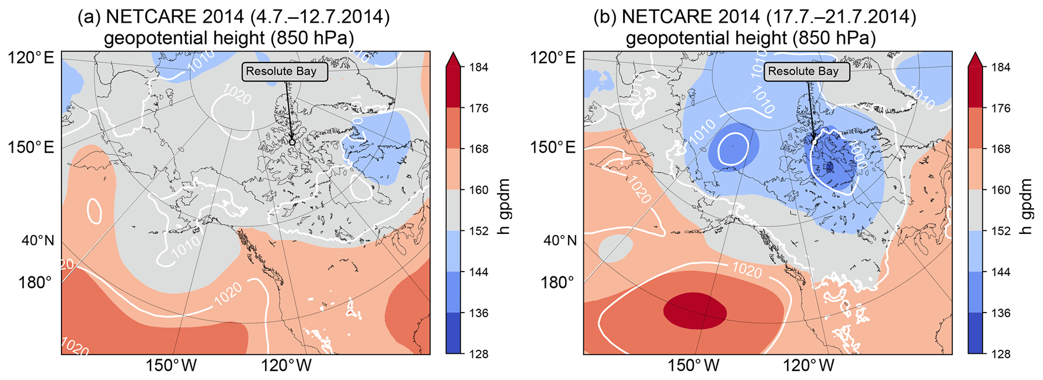
Figure 2 Mean geopotential height at 850 hPa in geopotential decameters (gpdm) for the period from 4 to 12 July 2014 (a) and for the period from 17 to 21 July 2014 (b).

4.2 NETCARE 2015

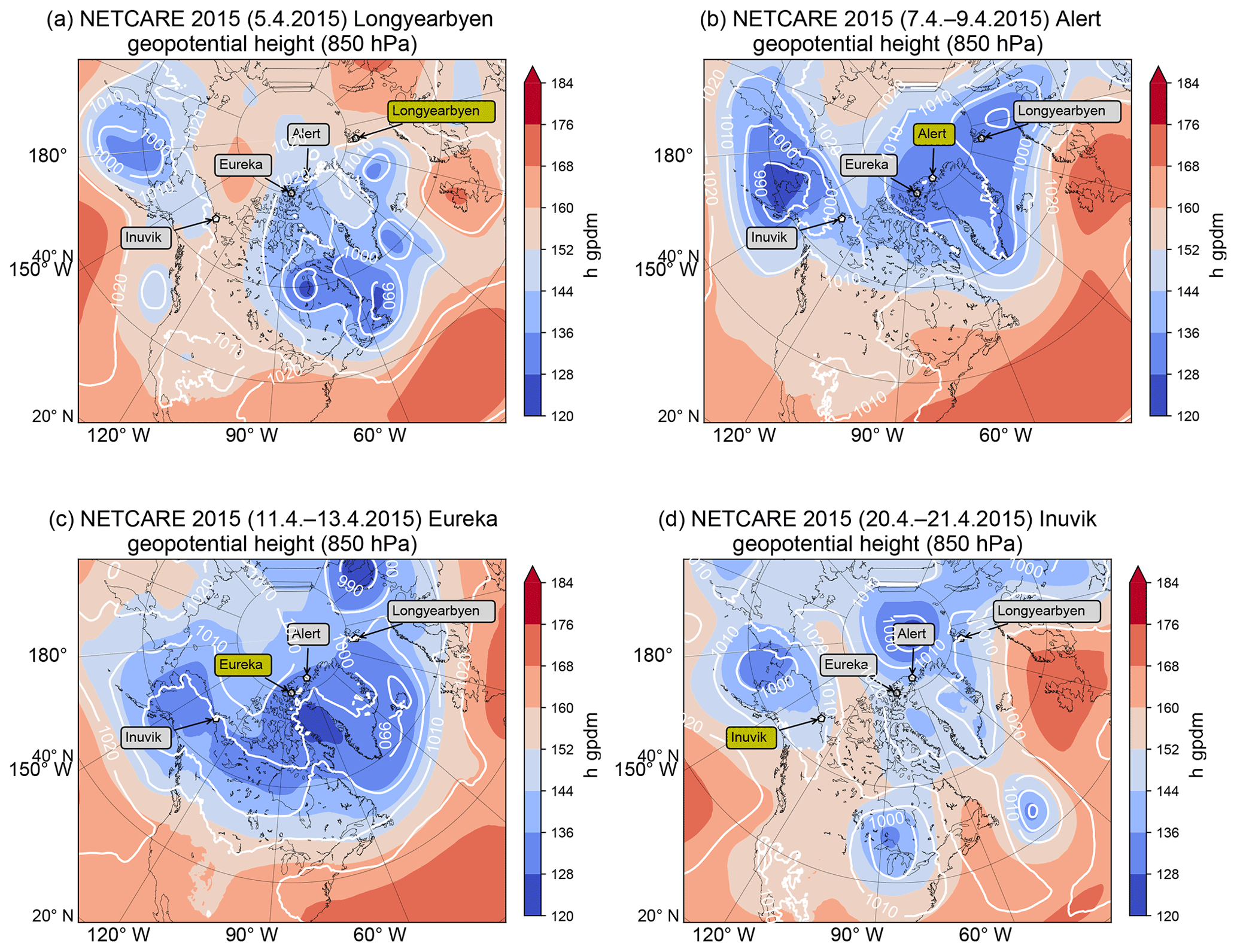
Figure 3 Mean geopotential height at 850 hPa in geopotential decameters (gpdm) from 5 April 2015 (a), from 7 to 9 April 2015 (b), from 11 to 13 April 2015 (c), and from 20 to 21 April 2015 (d). Our flight location for each time period is marked in yellow.

The aircraft were based at four different locations, namely Longyearbyen (Norway), Alert, Eureka (both Nunavut, Canada), and Inuvik (Northwest Territories, Canada), allowing for wider coverage of the entire Arctic. Figure 3 shows mean geopotential height at 850 hPa over the time interval of the measurements in the respective region. At the time of the first flight of the campaign in Longyearbyen (5 April; see Fig. 3a), Spitsbergen was under a quite stable high-pressure influence with almost no clouds and only weak winds. During the measurements in Alert the meteorological situation was dominated by a pool of cold air centered above Ellesmere Island to the southwest of Alert. A cyclonic flow was established around this cold air, guiding low-pressure systems around the cold pool and thus preventing midlatitude air masses from influencing the high Arctic lower troposphere. Stable conditions with almost clear sky facilitated airborne measurements on four research flights between 7 and 9 April during this period (see Fig. 3b). After the transfer to Eureka on 10 April two research flights were performed in almost the same meteorological conditions as in Alert. When the surface low started moving south over Baffin Bay from 13 April onward (see Fig. 3c) strong northerly and northeasterly winds in the lower troposphere influenced the measurement regions. The warmer flow was guided from southern areas over open water around the low-pressure center and was associated with moisture transport to the land, leading to cloud formation and fog, which impeded research flights out of Eureka. In the following days a low-pressure system started intensifying north of Greenland and maintained the low-level moist northerly flow. The last flights of the campaign were conducted in Inuvik between 20 and 21 April. After the ferry from Eureka to Inuvik on 17 and 18 April high-pressure influence was prevalent in Inuvik. At the time of the research flights a low-pressure system located over Alaska fostered a southerly and south easterly flow into the Inuvik area, favorable for midlatitude air masses to enter the measurement region (see Fig. 3d). A detailed description of the air mass history corresponding to the meteorological situation is given in the Supplement (Figs. S1 and S2).

5 Results

5.1 Trace gas observations

Based on the meteorological situation and transport regimes discussed above, we expect a significant influence of air mass history on the mixing ratios of CO and CO₂. Both species show latitudinal and vertical gradients (see Fig. 4), and both are affected by anthropogenic pollution, making them ideally suited for the identification of pollution events affecting the Arctic background. Our aircraft-based measurements of CO and CO₂ are in very good agreement with ground-based observations (see Fig. 4). In April 2015 trace gas levels are in general higher compared to July 2014. The observed change in trace gas levels between spring and summer reflects the typical seasonal cycle of these two species in the Arctic.

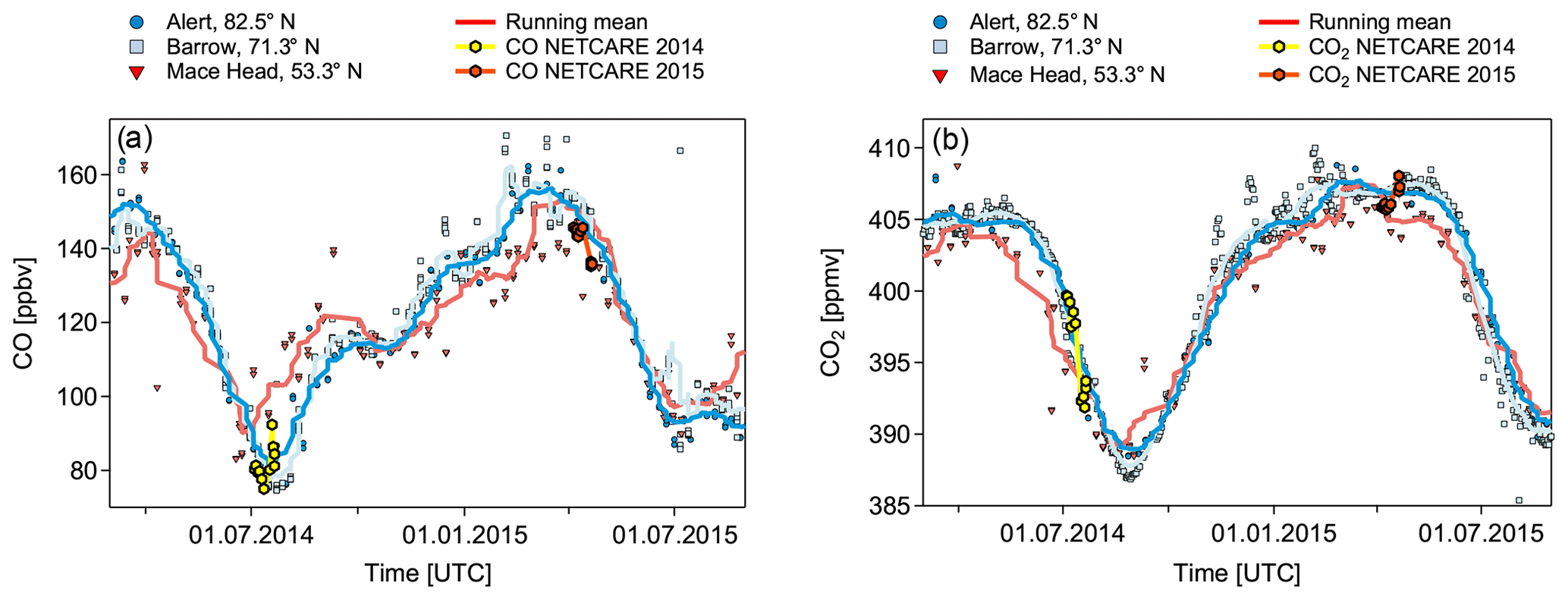
Figure 4 CO (Dlugokencky et al., 2018) (a) and CO₂ (Petron et al., 2018) (b) seasonal cycle based on NOAA ground-based measurements in Alert (Canada), Barrow (Alaska), and Mace Head (Ireland) for the years 2014 and 2015. Running means (10 points) are shown for the respective station data (symbols). Mean aircraft data for altitudes lower than 200 m for individual flights are overlaid. Error bars (yellow and orange shading) for the aircraft data are too small to be visible. NETCARE 2014 data are in yellow and NETCARE 2015 data are in orange.

The high Arctic CO seasonal cycle shows a maximum in late winter–early spring and a minimum during late summer. This seasonal maximum reflects the transport of anthropogenic pollutants – mainly from fossil fuel burning – from northern Europe and Siberia into the high Arctic lower troposphere during winter (Klonecki, 2003; Stohl, 2006). Since photochemically produced OH is absent during wintertime due to the lack of sunlight, CO in the high Arctic has no significant sink, which results in a longer chemical lifetime on the order of months. Hence, CO increases over the course of the winter, in particular within the polar dome that furthermore expands over potential emission regions in more southern latitudes (Novelli et al., 1998; Engvall et al., 2008). As soon as sunlight returns during late February and early March there is a sharp transition between 24 h polar night and 24 h polar day. The increasing concentration of OH leads to increased oxidation of CO and a shorter lifetime on the order of weeks (Dianov-Klokov and Yurganov, 1989; Holloway et al., 2000). During the transition from spring to summer (April to June) photochemical activity in the Arctic and smaller midlatitude emissions of CO directly into the polar dome lead to decreasing CO in the Arctic until a minimum is reached at the end of the summer (Barrie, 1986; Klonecki, 2003; Engvall et al., 2008).

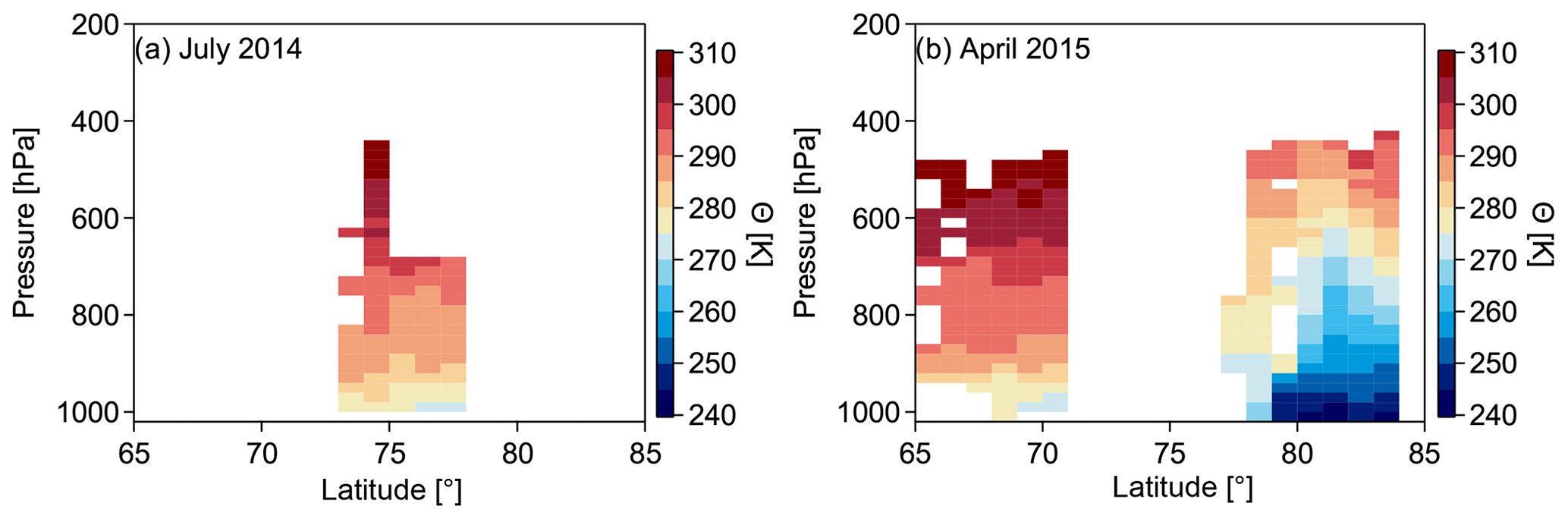
Figure 5 Potential temperature Θ as a function of latitude and pressure binned in steps of 1^∘ latitude and 20 hPa pressure for July 2014 (a) and April 2015 (b). Note the dome-like structure during April 2015 (NETCARE 2015), which is virtually absent for the Resolute Bay data during July 2014 (NETCARE 2014).

The CO₂ seasonal cycle in the Northern Hemisphere is mainly controlled by carbon uptake and release processes of the biosphere (Keeling et al., 1996; Forkel et al., 2016). Whereas during the summer months the CO₂ seasonal cycle reaches its minimum due to photosynthetic carbon uptake by vegetation, respiration of the biosphere is prevalent during wintertime. Particularly in Arctic winter, the absence of sunlight allows for a build-up of CO₂ concentrations. However, meridional CO₂ transport into the high Arctic by synoptic weather disturbances plays a critical role for the seasonal cycle and dominates over local atmosphere–biosphere fluxes (Fung et al., 1983; Parazoo et al., 2011; Barnes et al., 2016). As a result, the synoptic-eddy-driven meridional transport reduces the seasonal cycle in midlatitudes and amplifies it in polar regions, leading to a meridional CO₂ gradient (Parazoo et al., 2011).

5.2 The polar dome location

The polar dome can be conceptualized vertically as the region below upward-sloping isentropes and horizontally as the region north of where isentropes intersect with the surface. Figure 5 shows the observed potential temperature (Θ) distribution as a zonal mean for the respective campaigns. Potential temperature was calculated from temperature and pressure measurements onboard the Polar 6 aircraft. A dome-like structure of the isentropes is visible for April 2015 (NETCARE 2015). Minimum potential temperatures lower than 275 K were only present in the high Arctic lower troposphere north of 70^∘ N. In contrast, a dome-like structure is hardly visible for July 2014 (NETCARE 2014). Only below 950 hPa and north of 75^∘ N were Θ values of 275 K observed. Our observations are in agreement with previous studies showing that during the summer months the extent of the polar dome is much smaller compared to the wintertime (Klonecki, 2003; Stohl, 2006; Jiao and Flanner, 2016).

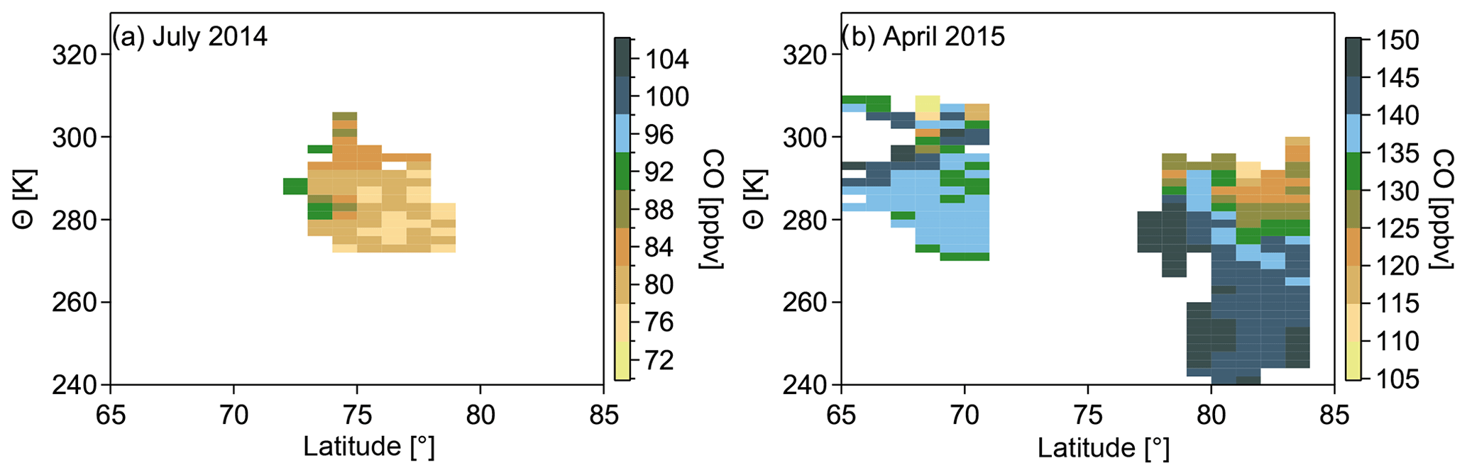
Figure 6 CO distribution binned by latitude and potential temperature for July 2014 (a) and April 2015 (b). The color code represents the average CO mixing ratio calculated from all data points in the respective 1^∘ latitude and 2 K bin interval. Note that only background mixing ratios are shown now. Polluted air masses are identified and filtered when the average background distribution is exceeded by 2σ.

If we now use potential temperature as the vertical coordinate, air masses within the polar dome associated with the coldest potential temperatures should separate from other regions. This separation is evident in Fig. 6, particularly for the April 2015 measurements (b). The color code in Fig. 6a and b represents the average CO background mixing ratio calculated from all data points within the respective bin interval. In our analysis of the polar dome we only use background trace gas mixing ratios. We exclude polluted air masses if the mean background CO mixing ratio is exceeded by 2 standard deviations. In April 2015 (Fig. 6b) the northernmost latitudes exhibited the largest CO values of 140–150 ppbv for potential temperatures lower than 275 K. At higher isentropes typical CO values range from 100 to 135 ppbv. At these higher potential temperatures, the larger variability of CO mixing ratios indicates different source regions contributing to the observations, which is in particular observed for the lower latitudes. In the distribution for the summer campaign (Fig. 6a) a region of rather uniform low CO is evident north of 75^∘ N and below 290 K. Mixing ratios south of 75^∘ N and above 290 K tended to be more variable and in general larger than within the more northern region. Again, the increased variability results from different air mass origins associated with different levels of CO. In both measurement campaigns, we observed a distinct transition between the northernmost lower troposphere and regions with lower latitudes and larger potential temperatures. This transition indicates a transport barrier for air masses to reach the high Arctic lower troposphere. We hypothesize that those regions north of 75^∘ N showing the lowest CO mixing ratios during July 2014, as well as the largest during April 2015, represent the polar dome, whereas the rest of the measurements were collected outside the polar dome.

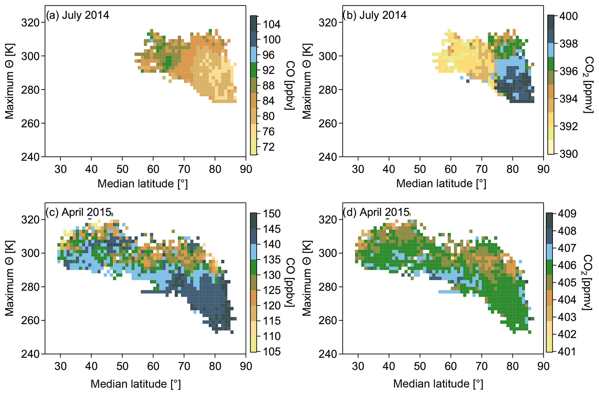
Figure 7 Panels (a)–(d) show trace gas distributions in the maximum potential temperature and median latitude coordinate system. The median and maximum values were derived from every 10 d trajectory calculated along the flight track. The color code is representative for the average CO (CO₂) value calculated from all data points within one bin interval. The trace gas mixing ratio is the measured value that is assumed to stay constant along the respective trajectory for each measured data point every 10 s.

The trace gas distribution in Fig. 6 only shows a snapshot of the actual situation at the time and the location of the measurement. We used 10 d backward trajectories to take into account different transport pathways to the Arctic and the residence times of air masses inside the polar dome area, which is likely higher than residence times in areas outside the polar dome. We display the CO and CO₂ distribution in a maximum potential temperature versus median latitude coordinate system. Maximum potential temperature and median latitude were derived along every individual trajectory. Median latitude allows for a separation between high Arctic air masses and air masses from midlatitudes. Air parcels isolated in the polar dome region should stay at high median latitudes, whereas air masses extending over a larger meridional distance show a more southern median latitude. Maximum potential temperature further allows us to account for the diabatic descent of air masses during transport. In the maximum potential temperature vs. median latitude coordinate system those air masses inside the polar dome region exhibit the lowest maximum potential temperatures and at the same time the largest median latitudes, and they are thus separate from air masses outside the polar dome. Furthermore, the polar dome is dynamically well isolated from the surrounding troposphere as discussed earlier. Hence, air parcels inside the polar dome are in general not affected by strong midlatitude CO sources and should show a relatively small CO variability. Therefore, we remapped the CO data to the median latitude and maximum potential temperature along the trajectory to identify transport regimes and the effect of the transport barrier at the polar dome (see Fig. 7a and c). The majority of trajectories with relatively low CO mixing ratios are confined by the 305 K isentrope and 70^∘ N as evident in Fig. 7a for July 2014. For April 2015 (Fig. 7c) an area with relatively higher CO is located north of a latitude of 65^∘ N and below a potential temperature of around 280 K. These findings are supported by the CO₂ distribution in the same coordinate system displayed in Fig. 7b and d, which show similar boundaries. Hence, gradients of CO and CO₂ establish at these boundaries. In this study these chemical gradients are used to derive a tracer-based definition of the polar dome boundary for the two NETCARE measurement campaigns during July 2014 and April 2015. Next, we determine the location of the polar dome boundary based on trace gas gradients.

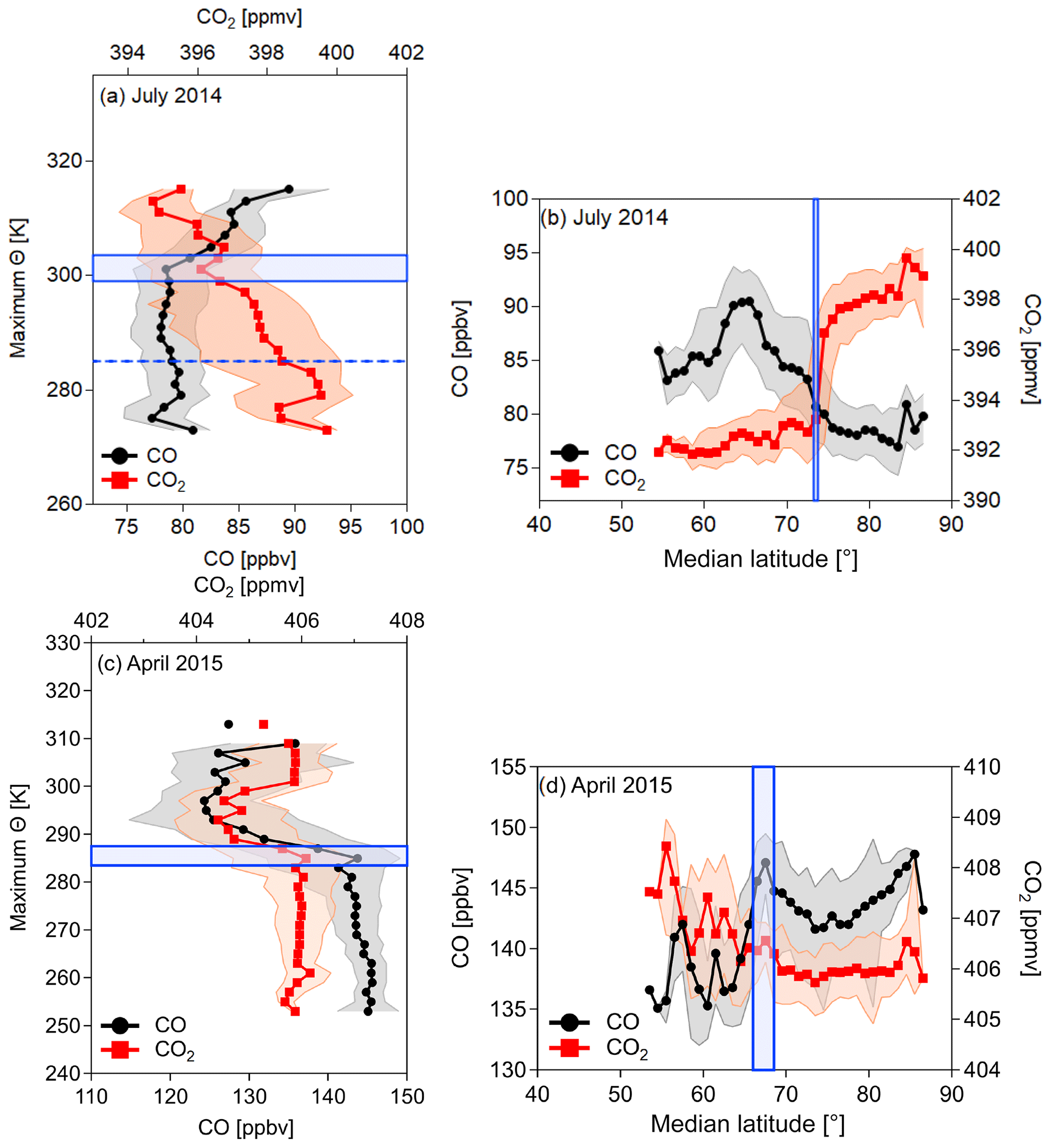
Figure 8 Medians of CO and CO₂ as a function of median trajectory latitude and maximum trajectory potential temperature (for details, see the text). Median values for the vertical profiles were only calculated north of 75^∘ N for July 2014 (a) and north of 65^∘ N for April 2015 (c) because latitudinal gradients indicate a dome boundary north of these median latitudes. At lower latitudes transport and mixing homogenize these gradients (see Fig. 7). For both NETCARE campaigns the median horizontal values were derived only below 300 K (b and d). The blue bar marks the latitude and the potential temperature interval of the strongest change in the tracer mixing ratio, which is interpreted as the transition zone of the polar dome boundary. The shaded area in all figures represents the 1σ standard deviation.

Trace gas gradients

In July 2014 both CO and CO₂ show a latitudinal gradient across the isentropes for maximum potential temperature levels of Θ<305 K (see Fig. 7a and b). In particular, CO₂ shows a strong increase from values around 393 to 398 ppmv toward high latitudes in the median latitude range of 70 to 75^∘ N. For CO, a decrease from about 83 to 78 ppbv in this latitude range is also evident. In contrast to CO₂ the large variability of CO at lower median latitudes reflects a larger variability of potential source regions, which in turn partly masks the CO gradient. Above 305 K trace gas gradients are weak or absent, indicating rapid isentropic mixing from lower latitudes. We calculate isentropic trace gas gradients in layers of 2 K for the maximum potential temperature as the vertical coordinate in Fig. 7 to derive the horizontal polar dome boundary. For every 2 K altitude interval we determine the latitude of the strongest trace gas gradient. Below 305 K isentropic trace gas gradients maximize around 73^∘ N. We finally use the median of these maximum gradient latitudes to define the polar dome boundary. If we derive a different median value for the maximum gradient for each of the two tracer species, we consider this difference to be the range of the polar dome boundary, which can be interpreted as a transition zone rather than a sharp boundary. For July 2014 the average horizontal polar dome boundary is a sharp transition at 73.5^∘ N (blue bar in Fig. 8b). The interquartile range denotes to 72.5–77^∘ N.

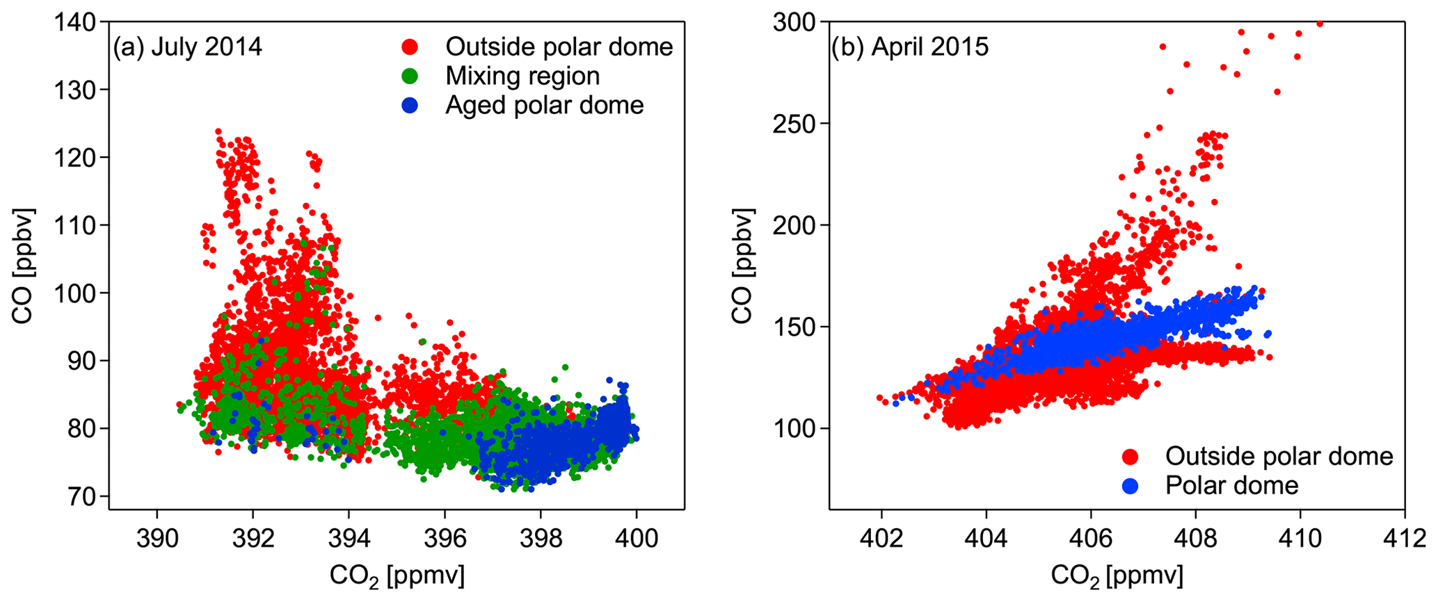
Figure 9 (a) Tracer–tracer scatter plot of all data points (background + pollution plumes) within the aged polar dome (blue), the mixing region (green), and outside the polar dome (red) for July 2014. (b) Tracer–tracer scatter plot of all data points (background + pollution plumes) within (blue) and outside (red) the polar dome for April 2015. To separate the different regions the tracer-derived polar dome boundaries are used. Boundary values for each region are summarized in Table 2.

The strongest vertical gradients of CO and CO₂ were determined at maximum potential temperature values of 299–303.5 K (blue bar in Fig. 8a; interquartile range: 297 to 304.5 K). These values for the upper polar dome boundary are relatively high given a surface value of potential temperature of typically 280 K in summer. A close inspection of the CO₂ distribution north of 73.5^∘ N (Fig. 7b) reveals two layers in the high Arctic separated at approximately 285 K. The vertical profile of CO₂ clearly shows the two layers (Fig. 8a). The fact that the vertical profile of CO does not show a clear separation indicates that rather pristine air masses dominate both layers, which have not experienced a strong pollution impact but rather a biogenic impact mainly affecting CO₂. If we additionally use this information, we can separate three distinct air masses. The region with the lowest potential temperatures (Θ<285 K) has small (large) mixing ratios of CO (CO₂) and is mostly isolated from midlatitude influence. These air masses are most likely remnants of the springtime polar dome, and we refer to this as the aged polar dome. Between 285 and 299 K the air masses still show signatures of the polar dome, while the influence from midlatitudes also increases, indicated by lower CO₂ mixing ratios. This region is capped in the vertical by the polar dome boundary between 299 and 303.5 K. Above and thus outside the polar dome, mixing ratios of both species clearly show characteristics of midlatitude influence. Similar values to those observed outside the polar dome were also found in the midlatitude lower troposphere, for example at the Mace Head observatory in Ireland (see Fig. 4). A summary of the values for the polar dome boundary and the boundaries of the three different regions for July 2014 can be found in Table 2.

The threefold structure of the high Arctic lower troposphere, based on the derived boundary values for each region summarized in Table 2, is further evident in the CO–CO₂ tracer–tracer correlation in Fig. 9a. More precisely, the aged polar dome (blue dots) seems to be a subset of the mixing region (green dots) indicated by a narrow group of data points at the end of the highest CO₂ and lowest CO mixing ratios. The aged polar dome region is furthermore clearly separated from the region outside (red dots). The green dots indicate the influence of mixing between dome air and extra-dome air and correspond to the mixing region in the high Arctic between 285 and 299 K (compare Fig. 7b).

The tracer-derived polar dome boundary for the April 2015 measurements was on average determined between 66.0 and 68.5^∘ N (blue bar in Fig. 8d; interquartile range: 65.0–69.5^∘ N) for the latitudinal value and between potential temperatures of 283.5 and 287.5 K (blue bar in Fig. 8c; interquartile range: 280.5 and 291.5 K). Values for the polar dome boundary are also summarized in Table 2 for April 2015. During spring the CO–CO₂ tracer–tracer correlation in Fig. 9b indicates at least three distinct branches. The separation of air masses between inside the polar dome and outside is based on the tracer-derived polar dome boundary (see Table 2). The red branch with the highest CO and CO₂ mixing ratios can be associated with pollution events observed during flights in Inuvik. In contrast, the red branch with the highest CO₂ but relatively low CO values corresponds to observations in the unpolluted lower troposphere in the Inuvik region. Both branches are clearly associated with air masses outside the polar dome, since measurements around Inuvik were mostly performed outside the determined polar dome boundary. In contrast, the blue branch represents the measurements inside the polar dome. These data points show different slopes, indicating different air mass properties. Within the polar dome region we observe a mixture of air masses, which is evident from the relatively broad range of CO₂ and CO values forming a mixing line in Fig. 9b. The lowest CO and CO₂ values inside the polar dome (blue) can be associated with the lowest maximum potential temperatures and thus the highest residence time within the dome area. Air masses with the highest CO and CO₂ mixing ratios but still inside the polar dome (blue) originate at lower latitudes. In fact, ground stations in the potential source region 2 weeks before the time of the measurement campaign show enhanced CO and CO₂ values in the range of the upper branch of the scatter plot of those data points inside the polar dome. The observed mixture of air masses is also reported by Willis et al. (2019), who observed an altitude-dependent composition and degree of processing of aerosol in the springtime polar dome. In their study, FLEXPART simulations suggest more southern source regions for those air masses with the highest potential temperatures within the polar dome. Furthermore, Schulz et al. (2019) determined an increase in refractive black carbon (rBC) and a decrease in the rBC mass mean diameter with potential temperature inside the springtime polar dome, which was also associated with different source regions contributing to the observations.

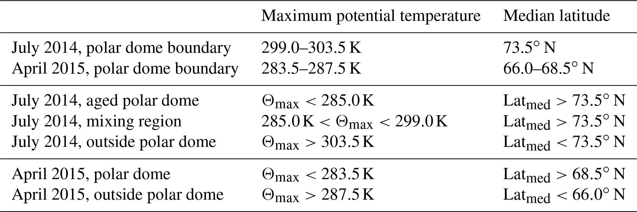
Table 2 Maximum potential temperature and median latitude values for the polar dome boundary. The boundary values used for separating the different regions identified for further analysis are also included.

5.3 Transport regimes

In order to analyze the processes dominating the recent transport history of observed air masses, we apply the phase-space diagram introduced by Binder et al. (2017). In this analysis, we determine the maximum change in potential temperature (ΔΘ) as the difference between the potential temperature at the time of the measurement (Θ₀) and the previous potential temperature minimum or maximum (Θ_min, Θ_max) along the trajectory. Depending on which absolute difference is larger, the air mass has either experienced diabatic heating ($\mathrm{\Delta }\mathrm{\Theta }=({\mathrm{\Theta }}_{\mathrm{0}}-{\mathrm{\Theta }}_{\min })>\mathrm{0}$) or cooling ($\mathrm{\Delta }\mathrm{\Theta }=({\mathrm{\Theta }}_{\mathrm{0}}-{\mathrm{\Theta }}_{\max })<\mathrm{0}$). An analogous analysis is made for the absolute temperature to determine if an air parcel predominantly gained or lost temperature before the measurement. This analysis allows us to cluster the data into the four categories shown in Figs. 10a–d and 11a–c. The changes in potential temperature and temperature along the trajectories, indicated by the clusters, can be associated with processes affecting the respective air mass. Sector 1 (ΔΘ<0, ΔT<0) mainly contains air masses that experienced diabatic cooling, which indicates thermal radiation, evaporation, or low-level transport over snow- or ice-covered regions (i.e., cold surfaces). In sector 2 (ΔΘ>0, ΔT<0) air masses gained potential temperature, which indicates an ascending air mass that is diabatically heated by, for example, solar radiation or condensation processes. Sector 3 (ΔΘ>0, ΔT>0) includes those air masses that experienced both an increase in temperature and potential temperature, probably due to solar insolation. Finally, sector 4 (ΔΘ<0, ΔT>0) combines air masses that lost potential temperature and gained temperature during transport. These air masses are diabatically cooled and thus experienced a descent. We apply this clustering approach to identify differences between observations in the different regions (polar dome, outside polar dome, etc.) and to study whether we can connect trace gas mixing ratios to the dominant process in a specific region. The different regions were separated based on the tracer-derived polar dome boundary (see Table 2) .

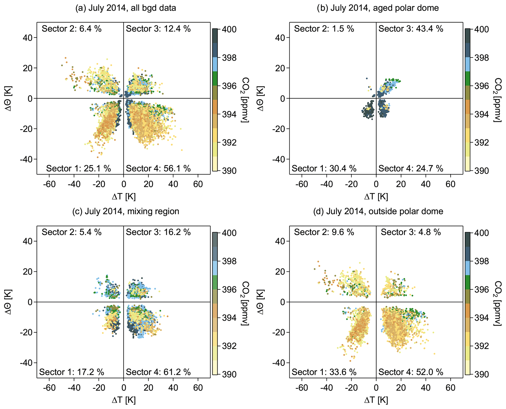
Figure 10 Phase-space diagram illustrating the maximum absolute change in temperature (ΔT) and potential temperature (ΔΘ) relative to the time of the measurement for July 2014. The color code denotes the CO₂ mixing ratio at the time of the measurement. Panel (a) shows all background data, panel (b) shows only those data corresponding to the aged polar dome, and panel (c) shows the data points within the mixing region, whereas panel (d) includes all data points outside the polar dome. To separate the different regions the tracer-derived polar dome boundaries are used (see Table 2).

Figure 11 Phase-space diagram illustrating the maximum absolute change in temperature (ΔT) and potential temperature (ΔΘ) relative to the time of the measurement for April 2015. The color code denotes the CO mixing ratio at the time of the measurement. Panel (a) shows all background data, panel (b) only shows those data corresponding to the polar dome, and panel (c) includes all data points outside the polar dome. To separate the different regions the tracer-derived polar dome boundaries are used (see Table 2).

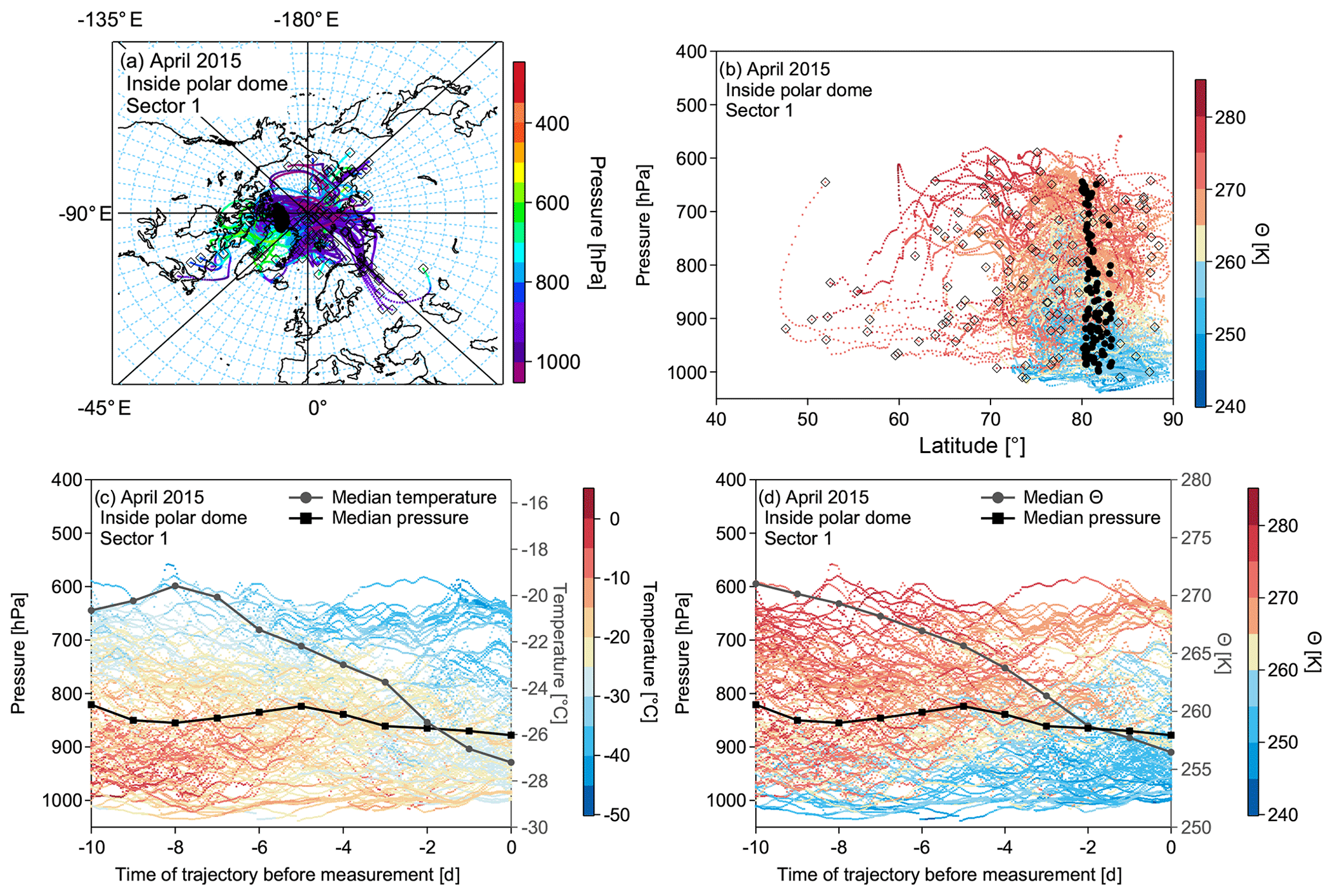
Figure 12 (a) Trajectories of the most dominant sector 1 for air masses inside the polar dome. The color code represents the pressure along the trajectories. (b) The same trajectories as in (a) as a function of pressure and latitude, color coded by potential temperature. In both (a) and (b) black circles denote the initialization point of the trajectory along the flight track. The black open squares show the position of the trajectory 10 d back in time. Panels (c) and (d) show height–time cross sections with pressure representing the altitude of the trajectories (left axis) for the trajectory evolution over the 10 d of travel, with the color code denoting the temperature (c) and potential temperature (d). The black line marks the median pressure of the trajectory cluster at the individual time steps, and the grey line indicates the median temperature and median potential temperature, respectively. Note that only every 20th trajectory is plotted for figure clarity.

For July 2014, three regions are of particular interest: (1) the aged polar dome, (2) the mixing region, and (3) the region outside the polar dome (see Fig. 10a–d). Within the aged polar dome sector 3 dominates, and thus solar insolation is important for heating the lowest levels. Air masses residing at the lowest altitude experienced diabatic heating, potentially resulting in a slow and shallow convective lift of the air masses prior to the time of the measurement. Equal contributions come from sectors 1 and 4, dominated by diabatic cooling through descent, low-level transport over cold surfaces, or evaporation. Almost none of the air masses are in sector 2, and thus a significant ascent of air masses within the aged polar dome hardly occurs. In contrast, outside the polar dome area sector 4 dominates and generally diabatic cooling occurs (sector 1 and 4). Thus, within the polar dome local near-surface diabatic processes seem to mostly affect the air masses; this effect is also evident in air mass composition. Observed CO₂ mixing ratios are highest in the aged polar dome associated with aged Arctic air and negligible midlatitude influence. Outside the polar dome, air masses have been transported into the Arctic and descended due to radiative cooling. The associated CO₂ mixing ratios of these air masses are significantly lower and can be attributed to more midlatitude regions. Air masses associated with sector 4 experience descent once they have reached the high Arctic at higher altitudes. This can be regarded as a typical transport pathway during the summer with a fast uplift of air masses at midlatitudes within convective and frontal systems, followed by a northward movement and finally a descent into the high Arctic lower troposphere. Air masses in the mixing region are even more dominated by sector 4. Within this mixing region, trace gas concentrations still show dome-like characteristics, and low-level processes seem to dominate over episodes of midlatitude transport associated with air masses with lower CO₂ concentrations. Results for CO confirm the derived transport history for July 2014. A more detailed analysis of the physical processes along the air mass trajectories can be found in the Supplement (Figs. S3, S4, and S5) to this paper.

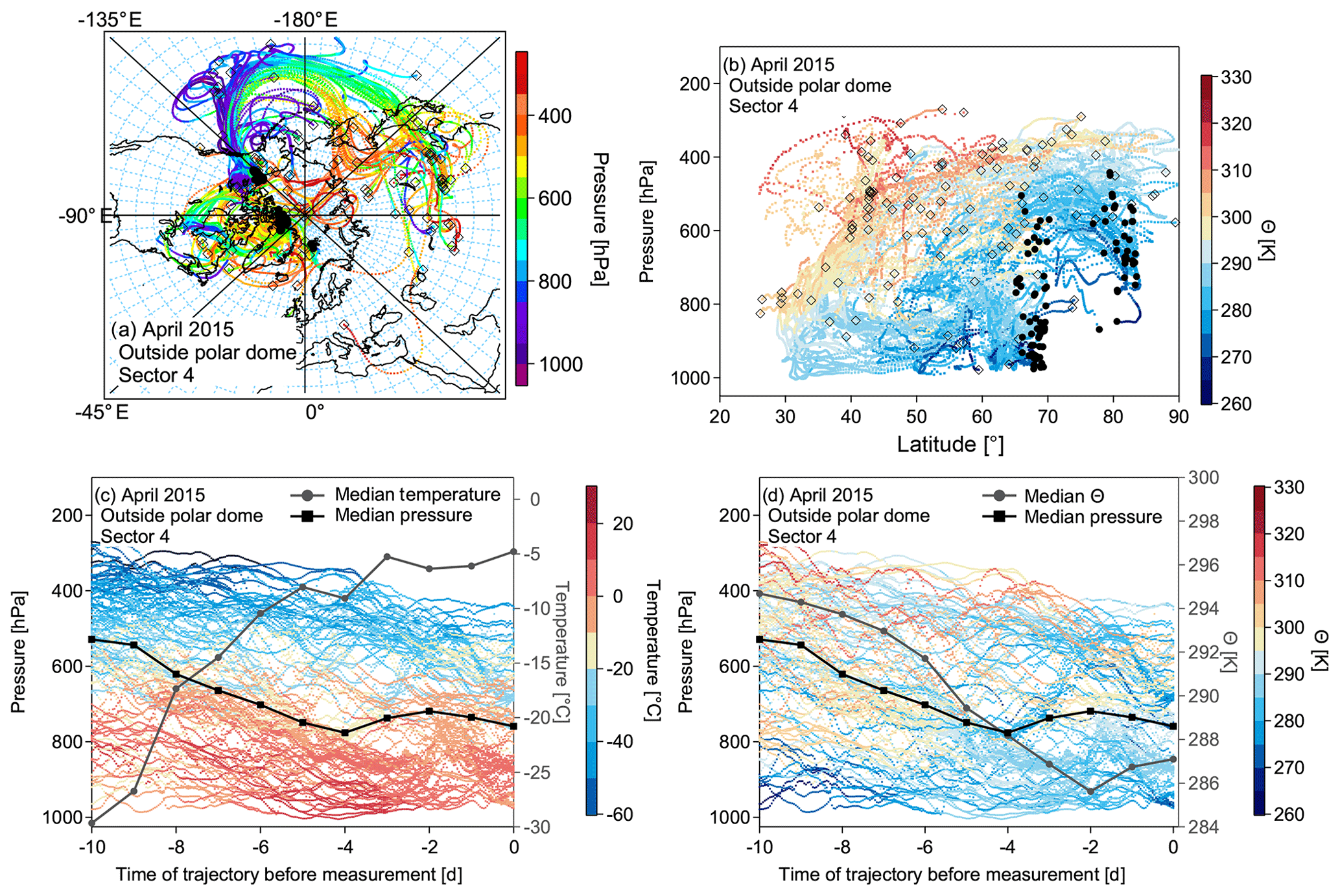
Figure 13 (a) Trajectories of the most dominant sector 4 for air masses outside the polar dome. The color code represents the pressure along the trajectories. (b) The same trajectories as in (a) as a function of pressure and latitude, color coded by potential temperature. In both (a) and (b) black circles denote the initialization point of the trajectory along the flight track. The black open squares show the position of the trajectory 10 d back in time. Panels (c) and (d) show height–time cross sections with pressure representing the altitude of the trajectories (left axis) for the trajectory evolution over the 10 d of travel, with the color code denoting the temperature (c) and potential temperature (d). The black line marks the median pressure of the trajectory cluster at the individual time steps, and the grey line indicates the median temperature and median potential temperature, respectively. Note that only every 20th trajectory is plotted for figure clarity.

In April 2015 the picture is quite different (see Fig. 11a–c). Inside the polar dome diabatic cooling dominates, in particular in sector 1. This is caused by diabatic descent due to radiative cooling in the absence of sunlight. In addition, low-level transport over cold surfaces significantly contributes to transport into the high Arctic. The associated mixing ratios of CO show rather large values that can be explained by the accumulation of anthropogenic pollution from inner Arctic and high northern midlatitude sources during the winter months. In the absence of sunlight chemical loss is reduced, leading to an increase in the CO atmospheric lifetime. Air masses within the polar dome are quite efficiently isolated from any significant southern midlatitude influence. In contrast, outside the polar dome the picture is more diverse. Sector 4 dominates, and thus diabatically cooled air masses potentially associated with the tendency to descend are observed. Input from various remote sources leads to stronger variations in the CO mixing ratio. However, all sectors contribute with more than 10 % to the observed distribution. Our interpretation of air mass transport history is confirmed by the results from CO₂.

Based on results from the phase-space diagrams, we further analyzed the trajectories of the individual clusters. This allows for a more detailed analysis of the physical processes along the trajectory. We compare the two most dominant sectors for the April 2015 measurements in Figs.12a–d and 13a–d for air masses inside and outside the polar dome, respectively. Sector 1 is mostly dominated by air masses confined to the central Arctic at all altitude levels (see Fig. 12a and b). The air masses show a weak descent during the 10 d period before the measurements but experience a very pronounced decrease in temperature and potential temperature (see Fig. 12c and d; median trajectory cluster temperature). In contrast, air masses outside the polar dome, dominated by sector 4, contain contributions from different airstreams. Air masses originate at different altitudes in the central Arctic, at low levels over the Pacific Ocean, and from the upper troposphere over Asia. Air masses in this cluster are characterized by a significant increase in median temperature and decrease in median potential temperature, indicating a descending trend, which is confirmed by decreasing median pressure over the time of travel. Low-level transport over the Pacific is associated with a low-pressure system over Alaska. Those air masses arrive at the polar dome boundary in the measurement region after experiencing a weak net cooling over Alaska.

We conclude that air masses within the aged summertime polar dome are mostly confined to the boundary layer, while they experienced a weak diabatic warming due to insolation in July 2014 during NETCARE. In the mixing region and outside the polar dome, diabatic cooling and a continuous descent are observed. Within the polar dome in April 2015 during NETCARE mostly near-surface processes (diabatic cooling due to the flow over cold surfaces) dominate the recent transport history of air masses in the lower polar dome. Air masses in the upper polar dome experience a very slow descent induced by radiative cooling. Outside the polar dome, air masses mostly arrive at higher potential temperatures in the Arctic and experience a continuous slow descent with increasing temperatures but only weak diabatic cooling.

5.4 Chemical properties of the transport regimes

5.4.1 Trace gases

Using the tracer-derived polar dome boundary we compare the composition of air masses within the polar dome region and the surrounding region (Table 2). We make this comparison based on the probability density functions (PDFs) of measured trace gases CO and CO₂ for July 2014 (see Fig. 14a and b) and April 2015 (see Fig. 14c and d).

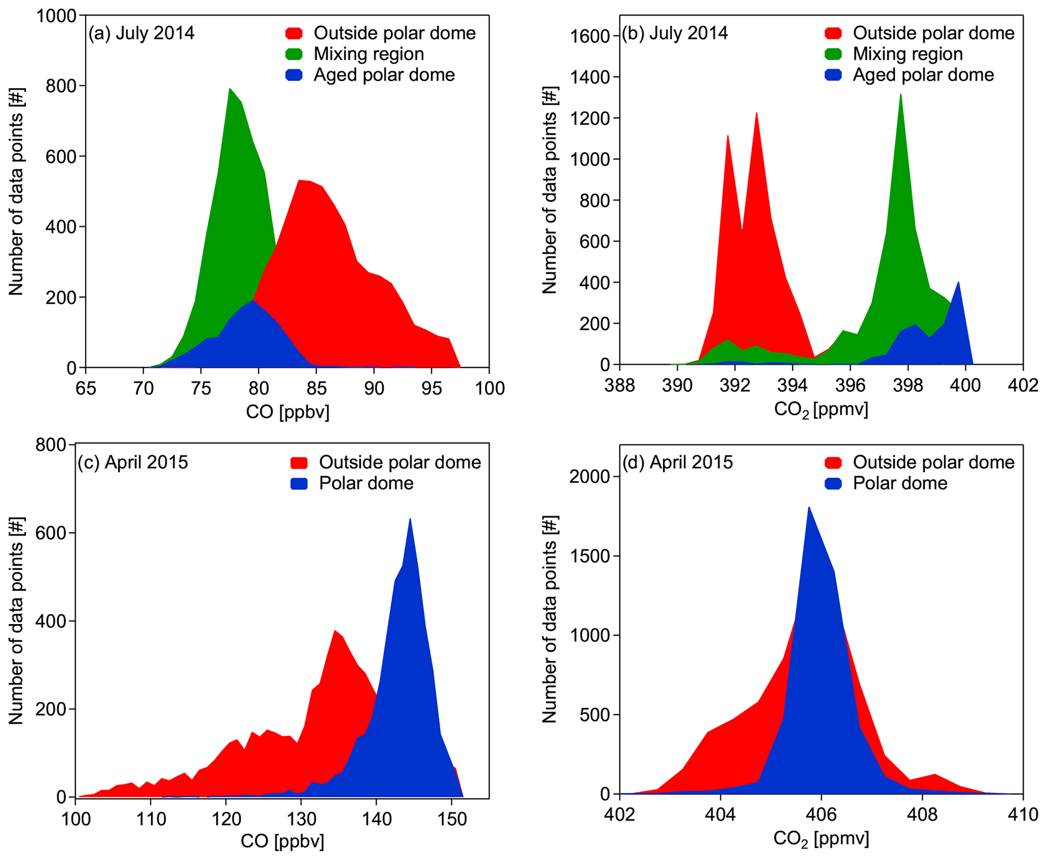
Figure 14 Probability density functions (PDFs) of all CO (a, c) and CO₂ (b, d) background measurements during July 2014 (a, b) and April 2015 (c, d). The median latitude and maximum potential temperature coordinates along the 10 d back trajectories were used for the separation between inside and outside the polar dome using the tracer-derived polar dome boundaries (see Table 2).

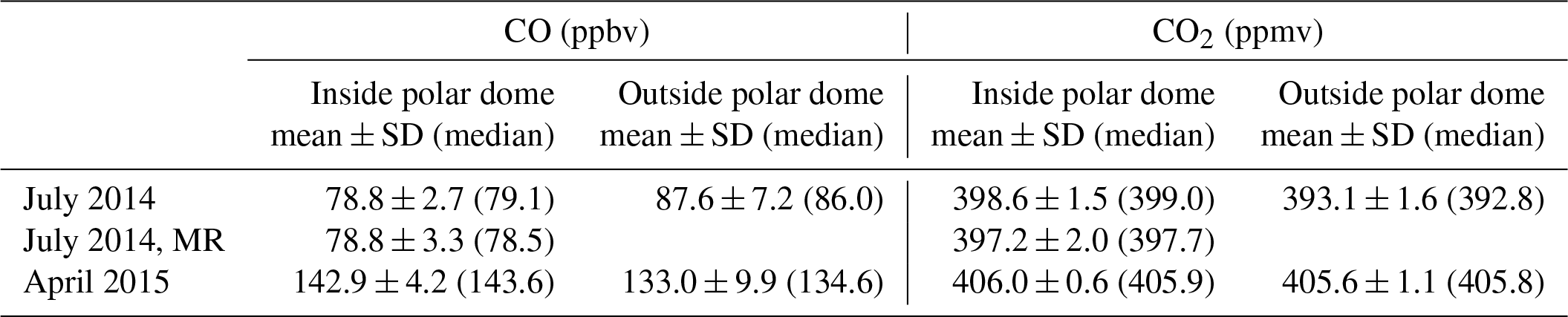
For July 2014 the three different regions identified in Sect. 5.2.1 are confirmed by the respective PDFs for both species. The aged polar dome and the mixing region show a quite similar distribution for both species, except differences in the mode of the PDF, and are well separated from data outside the polar dome area. Whereas the absolute CO value inside the aged polar dome and the mixing region is lower compared to the area outside the polar dome, the CO₂ average mixing ratio within the polar dome is higher compared to the surroundings, as summarized in Table 3. This finding can be explained by the seasonal cycle of these two species and their zonal gradients (see data from NOAA ground-based measurements in Fig. 4b). The minimum of the seasonal cycle of CO₂ in the Arctic and the midlatitudes is reached at the end of the summer, typically during September. However, the onset of carbon uptake by vegetation in the midlatitudes starts earlier compared to the high Arctic where less vegetation is present. At the same time the overall burden of CO₂ in the Arctic lower troposphere is to a large extent controlled by transport processes (Fung et al., 1983; Parazoo et al., 2011; Barnes et al., 2016). Midlatitude air with relatively low CO₂ mixing ratios is transported to the high Arctic, in particular during the second phase of the campaign. But, as the polar dome acts as a transport barrier for those air masses, exchange of high Arctic lower tropospheric air with midlatitude air is reduced, leading to the observed PDF for CO₂. Under 24 h daylight conditions and with only a few inner Arctic sources of pollution, CO concentrations reach their minimum in the high Arctic in late summer. Air masses transported into the high Arctic from more southern regions are expected to have relatively high CO mixing ratios due to the seasonal cycle of CO that has a stronger amplitude in the Arctic compared to midlatitudes (see Fig. 4a). The increased midlatitude influence in the second half of the campaign enhanced the CO burden in the Arctic troposphere, whereas the inner Arctic air masses observed in the first half of the campaign were dominated by photochemically aged low CO air.

Table 3 Mean and median mixing ratios of CO and CO₂ inside and outside the polar dome area using the tracer-derived polar dome boundaries. The respective mixing ratios were calculated based on the minimum latitude and maximum potential temperature coordinates. Note that for the July 2014 dataset the mixing ratios of the mixing region (MR) are also included in the table.

We observed a strong link between trace gas distributions and the observed change in the synoptic situation from a more high-pressure-controlled regime to a synoptically active regime. Based on the trajectory simulations, an increased midlatitude influence was observed, which in turn influenced the general concentration level of the trace gases CO and CO₂ (see Supplement Fig. S6). CO increased from 77.9±2.5 to 84.9±4.7 ppbv. At the same time CO₂ decreased from 398.2 ± 1.0 to 393.8 ± 2.3 ppmv. Furthermore, increased variability in CO and CO₂ was observed, indicating enhanced entrainment of polluted midlatitude air masses into the high Arctic. Some of the trajectories originating from outside the polar dome area pass the Northwest Territories at low altitude, potentially within the boundary layer, where extensive biomass burning occurred during the time of the measurements and before. Accordingly, increased aerosol concentrations during the second half of the campaign were reported by Burkart et al. (2017).

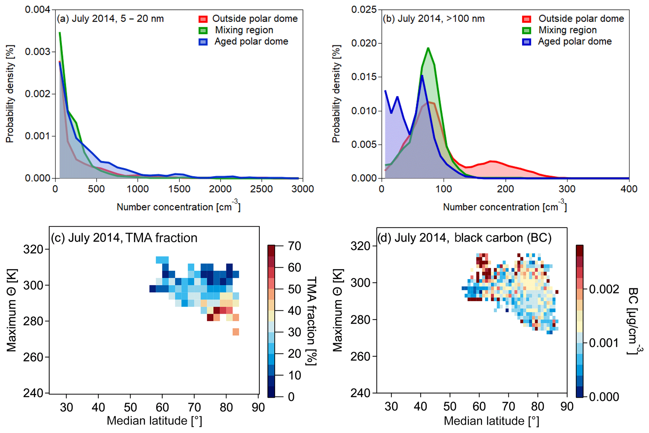
Figure 15 Normalized probability density functions for particles with diameters between 5 and 20 nm (a) and larger than 100 nm for July 2014 (b). The color code represents the three different regions identified during the polar dome analysis. Panel (c) shows the distribution of the fraction of particles containing trimethylamine with respect to the total amount of particles measured by single-particle mass spectrometry (Köllner et al., 2017) in the maximum potential temperature and median latitude coordinate system. Note that due to particle spectra statistics the resolution of the median latitude and maximum potential temperature interval is reduced compared to the refractory black carbon distribution (BC) shown in panel (d). There is a slight enhancement in BC south of (80^∘ N) within the polar dome, which is most probably due to fresh local pollution.

Using the polar dome boundary values listed in Table 2, Fig. 14 shows probability density functions for all CO (c) and CO₂ (d) background measurements during April 2015. Based on the PDFs, the difference in tropospheric trace gas composition within and outside the polar dome region is clearly visible for CO but less distinct for CO₂. Average values for both species in the respective regions are also summarized in Table 3. In general, the distributions of CO and CO₂ are much narrower within the polar dome region, and CO mixing ratios tend to be higher within the polar dome. For CO₂ the mean mixing ratio is quite similar within and outside the polar dome. However, a difference in the general distribution is observed. The reason for a less distinct separation between inside and outside the polar dome area is indicated by the seasonal cycles shown in Fig. 4a and b. CO₂ concentrations are on a plateau in spring, with reduced concentration changes with time and reduced latitudinal gradients. The CO mixing ratio has already started to decrease at the time of our measurements. However, the extent of the polar dome is much larger during the winter months and spring compared to the summer months. Hence, more influence from northern midlatitudes and more midlatitude pollution sources are expected inside the dome area. CO-rich air masses originate in cold regions of Eurasia and are able to reach the high Arctic lower troposphere where they are trapped during winter and early spring (Klonecki, 2003; Stohl, 2006; Jiao and Flanner, 2016). This leads to relatively large CO levels inside the polar dome compared to the region outside. In contrast, air masses from more southern midlatitudes that are transported above the polar dome have already experienced the photochemical loss of CO near their source region.

5.4.2 Aerosol

Having defined the polar dome based on trace gas gradients allows for a more detailed study of aerosol associated with the different air masses. Efficient wet removal and less efficient transport from lower latitudes lead to generally low aerosol concentrations (Stohl, 2006; Engvall et al., 2008) in the Arctic lower troposphere during summer. This is consistent with results in Fig. 15a and b. Observations of elevated levels of accumulation-mode particles (N_>100) can be associated with regions outside the polar dome and subsequent transport to the measurement region. In parallel, regions within the polar dome were characterized by N_>100 smaller than 100 cm⁻³. In contrast, number concentrations of ultrafine particles (N₅₋₂₀) occasionally showed larger values within the polar dome compared to outside (Fig. 15a), indicating the formation of ultrafine particles that occurred within the polar dome region (Burkart et al., 2017). Exemplary for aerosol composition, particulate trimethylamine (measured by single-particle mass spectrometry) can be associated with sources within the polar dome (Fig. 15c), consistent with results in Köllner et al. (2017) and Willis et al. (2017). In contrast, the abundance of refractory black carbon can be linked to pollution sources outside the polar dome and subsequent transport to the measurement region (Fig. 15d) (Schulz et al., 2019). To conclude, the method introduced in this study is a useful tool to interpret Arctic aerosol observations in the context of transport processes and sources within and outside the polar dome region.

6 Discussion

Jiao and Flanner (2016) used the maximum zonal mean latitudinal gradient of 500 hPa geopotential height in the Northern Hemisphere to assess the impact of changes in atmospheric transport and removal processes due to climate change on the aerosol distribution in the Arctic. They deduced the polar dome boundary between 40 and 50^∘ N during January, which is further south compared to our tracer-derived values. However, their method does not account for the lower troposphere, which is essential for the diabatic processes affecting transport into the Arctic. For January, Klonecki (2003) determined a mixing barrier in the lower troposphere at 60^∘ N at longitudes between 60 and 105^∘ W for a short-lived artificial tracer (7 d atmospheric lifetime) emitted in North America and Europe. During summer they reported that the strong mixing barrier moves north following the location of the Arctic front. This is in the range of our horizontal polar dome boundary for the respective spring (66.0 to 68.5^∘ N) and summer (73.5^∘ N) season. In comparison to the location of the Arctic front determined in Klonecki (2003), our analysis seems to give a more northern boundary for both July 2014 and April 2015. Furthermore, Klonecki (2003) reported an increasing midlatitude influence with increasing altitude, in particular above 4 km of altitude, which supports our findings of the potential temperature boundary being below 300 K for both seasons (corresponding to an altitude below 4 km). An increasing midlatitude influence with altitude is also in line with the results from Stohl (2006), who also used the Arctic front as a marker for the polar dome boundary.

The most isolated regions of the polar dome, where air masses experience the longest residence times, span a bigger area during late spring (April 2015) compared to summer (July 2014). This is in good agreement with previous studies, since it is already known that the polar dome extent is much smaller during summer compared to the winter months, and processes and transport pathways controlling the composition of the high Arctic lower troposphere differ between the two seasons (Klonecki, 2003; Stohl, 2006; Law and Stohl, 2007; Engvall et al., 2008; Garrett et al., 2010; Fuelberg et al., 2010). Our measurements during spring confirm a larger extent of the dome compared to summer and rather represent winter conditions.

Stohl (2006) further defined an Arctic age of air and concluded that this age increased with decreasing altitude from 3 d between 5 and 8 km to around 1 week near the surface during the winter season (maximum 10 d in the North America region). During the summer season the air in the lowest 100 m of the troposphere is even older, with values of 13–17 d north of 75^∘ N. For a rough estimate of the upper limit of a transport timescale for midlatitude air traveling into the summer polar dome during NETCARE, we can estimate the time at which the average mixing ratio within the polar dome was last observed at midlatitude ground-based observatories (for example, Mace Head, Ireland). For CO₂, this suggests a transport time of around 3 weeks, which is of the order of magnitude of the summertime Arctic age of air in the lowermost troposphere reported by Stohl (2006). This estimate assumes a transport-controlled mixing ratio in the Arctic lower troposphere, which is justified by studies from Fung et al. (1983), Parazoo et al. (2011), and Barnes et al. (2016). Stohl (2006) further report that the Arctic troposphere is flushed on the timescales of 1–2 weeks in winter, whereas in summer the corresponding timescale is twice as long. Assuming a similarly short Arctic age during the spring season, this implies that above the polar dome air masses can be transported within days from midlatitude regions to the Arctic troposphere. Tracer concentrations will be further homogenized along isentropic surfaces when diabatic processes are slow compared to transport timescales (Klonecki, 2003). This is evident in a layer of similar CO mixing ratios above the polar dome observed in April 2015 (see Fig. 7c). During July 2014, increased diabatic heating due to convective and boundary layer heating in midlatitudes can lead to an uplift of air masses in midlatitudes and further transport into the Arctic, which prevents an isentropic distribution during summer (Fig. 7a and b). Several studies have analyzed the transport of midlatitude air masses into the Arctic troposphere above the polar dome along those pathways mentioned above, without explicit knowledge of the extent of the polar dome (Fuelberg et al., 2010; Roiger et al., 2011; Sodemann et al., 2011; Schmale et al., 2011; Brock et al., 2011; Ancellet et al., 2014, and references therein).

7 Summary and conclusion

In this study we defined the polar dome boundary based on tracer gradients. In July 2014, our results indicate that the horizontal polar dome boundary was located at a latitude of 73.5^∘ N. In the vertical a threefold structure established, with the strongest trace gas gradient observed in a potential temperature range between 299 and 303.5 K, separating air masses within the polar dome from those outside. A second weaker gradient was found at a potential temperature of 285 K. We identified the region below 285 K as the aged polar dome, with the highest degree of isolation and thus the longest residence time of air masses. Between 285 and 299 K a mixing region established. The mixing region shows significant characteristics of the polar dome region and is clearly separate from outside the polar dome (see Fig. 9a). In April 2015 the tracer-derived polar dome boundary was between 66.0 and 68.5^∘ N and in a potential temperature range of 283.5 to 287.5 K.

The processes dominating recent (10 d) transport history were analyzed using a phase-space diagram based on Binder et al. (2017). For air masses outside the polar dome, diabatic cooling and a temperature increase were prevalent in both spring and summer (see Figs. 10d and 11c). The associated transport pathway starts at midlatitudes where air masses are lifted in convective or frontal systems, followed by further northward motion towards the high Arctic, and finally descent into the lower Arctic troposphere. Previous studies have predominantly identified North America and Europe as the major source region associated with this pathway (Klonecki, 2003; Stohl, 2006). These source regions are also indicated from our observations (Figs. S1 and S2); however, a more comprehensive study of the source regions is beyond the scope of this paper. Furthermore, air masses within the polar dome can be identified based on their transport history. During spring, air masses experience predominantly diabatic cooling and lose temperature, which can be associated with low-level transport over cold surfaces. During summer an efficient cooling mechanism is missing. In fact, already cold air masses within the polar dome potentially experience a weak heating, thus leading to a conditionally unstable lower troposphere and potentially weak lifting. Diabatic cooling rates determined from the trajectories are in good agreement with the range of 1 K per day (radiative cooling) to several degrees per day (contact with cold and mostly snow-covered surface) reported for diabatic processes by Klonecki (2003).

Using our tracer-derived polar dome boundaries, PDFs of CO and CO₂ concentrations inside and outside the polar dome clearly show a difference in the distribution and also in the absolute value of the distribution maximum. Tracer–tracer scatter plots indicate that the polar dome is separate from the surrounding regions, with a different slope (April 2015) or a narrow group of data points at the end of the highest CO₂ and lowest CO mixing ratios (July 2014). The PDFs and the scatter plots confirm different air mass properties inside and outside the polar dome. For aerosol chemical composition, particles containing trimethylamine were enhanced inside the polar dome, indicating the influence of inner Arctic sources, whereas enhanced refractory black carbon concentrations outside the polar dome indicate remote sources of pollution.

We conclude that the differing chemical composition within and outside the polar dome allows for a trace-gas-gradient-based definition of the polar dome boundary. Phase-space diagrams helped to cluster the air masses based on differing heating and cooling rates. This gives further insight into the processes that control the recent transport history of the air masses within and outside the polar dome. The polar dome boundary derived in this study has already been used to study the source regions and chemical composition of aerosol within the polar dome (Schulz et al., 2019; Willis et al., 2019). Additionally, mixing and exchange processes along the polar dome boundary triggered by synoptic disturbances can be studied to shed light on additional pathways of midlatitude pollution that reaches the Arctic lower troposphere. A polar dome boundary derived from gradients of chemical tracers can be further used for a quantification of the influence of inner Arctic and remote sources of pollution affecting the Arctic lower troposphere in a changing climate.