Variability in a four-network composite of atmospheric CO₂ differences between three primary baseline sites

Spatial differences in the monthly baseline CO₂ since 1992 from Mauna Loa (mlo, 19.5^∘ N, 155.6^∘ W, 3379 m), Cape Grim (cgo, 40.7^∘ S, 144.7^∘ E, 94 m), and South Pole (spo, 90^∘ S, 2810 m) are examined for consistency between four monitoring networks. For each site pair, a composite based on the average of NOAA, CSIRO, and two independent Scripps Institution of Oceanography (SIO) analysis methods is presented. Averages of the monthly standard deviations are 0.25, 0.23, and 0.16 ppm for mlo–cgo, mlo–spo, and cgo–spo respectively. This high degree of consistency and near-monthly temporal differentiation (compared to CO₂ growth rates) provide an opportunity to use the composite differences for verification of global carbon cycle model simulations.

Interhemispheric CO₂ variation is predominantly imparted by the mlo data. The peaks and dips of the seasonal variation in interhemispheric difference act largely independently. The peaks mainly occur in May, near the peak of Northern Hemisphere (NH) terrestrial photosynthesis/respiration cycle. February–April is when interhemispheric exchange via eddy processes dominates, with increasing contributions from mean transport via the Hadley circulation into boreal summer (May–July). The dips occur in September, when the CO₂ partial pressure difference is near zero. The cross-equatorial flux variation is large and sufficient to significantly influence short-term Northern Hemisphere growth rate variations. However, surface–air terrestrial flux anomalies would need to be up to an order of magnitude larger than found to explain the peak and dip CO₂ difference variations.

Features throughout the composite CO₂ difference records are inconsistent in timing and amplitude with air–surface fluxes but are largely consistent with interhemispheric transport variations. These include greater variability prior to 2010 compared to the remarkable stability in annual CO₂ interhemispheric difference in the 5-year relatively El Niño-quiet period 2010–2014 (despite a strong La Niña in 2011), and the 2017 recovery in the CO₂ interhemispheric gradient from the unprecedented El Niño event in 2015–2016.

1 Introduction

Atmospheric CO₂ measurements are normally introduced into global carbon budgets as a “global growth rate … based on the average of multiple stations selected from the marine boundary layer sites with well-mixed background air …, after fitting each station with a smoothed curve as a function of time, and averaging by latitude band …” (Le Quéré et al., 2018). This approach encourages sampling at multiple locations to seek atmospheric confirmation of national/continental emission changes. Particularly in the Northern Hemisphere (NH), with more complicated geography and atmospheric circulation, the influence of continental emissions on marine boundary layer air can vary widely between sites.

A clearer indication of the global impact of regional emissions comes from sites demonstrating maximum spatial representation. In this case, global significance of biogeochemical CO₂ exchanges between the surface will be informed by their impact on validated baseline data with the least continental influence. Such baseline data are more directly relevant to changes in global ocean acidification and climate change, but places heightened demands on sampling criteria and calibration.

Sites selected to maximize spatial representation in their respective hemispheres, Mauna Loa (mlo, 19.5^∘ N, 155.6^∘ W, 3379 m) and South Pole (spo, 90^∘ S, 2810 m), also have the longest-term (multi-decadal) coherent trace gas monitoring data, based on flask sampling (Supplement S1). At these sites, and at Cape Grim (cgo, 40.7^∘ S, 144.7^∘ E, 94 m) since 1991, co-sampled baseline air has been analysed at three different laboratories, using four different methodologies summarized in Sect. 2.

To account for any persisting artefacts in the co-sampled data, we examine, for each method, inter-site differences in the published monthly baseline data from the three sites. The standard deviation in the average of the co-sampled differences provides a practical uncertainty estimate. A key advantage compared to the growth rate approach is that assumptions inherent in the growth rate smoothing (where for example 22-month smoothing is used to separate interannual and seasonal variations) are avoided so that in this study near-monthly effective time resolution is achieved.

The inter-site difference approach was used by Francey and Frederiksen (2016; FF16) to conclude that the suppression of the normal eddy component of interhemispheric (IH) CO₂ exchange in February–April 2010 contributed to the unprecedented 0.8 ppm step in the IH difference between 2009 and 2010. The dynamical anomaly was associated with a moderately strong El Niño leading to a NH build-up of CO₂ in 2010. FF16 supplementary information demonstrated a failure of atmospheric transport models of the carbon cycle to simulate the step.

The 2015–2016 El Niño was stronger and has also been associated with unprecedented behaviour in the global carbon cycle (elsewhere attributed to the terrestrial biosphere anomalies, e.g. Yue et al., 2017). However, Frederiksen and Francey (2018; FF18), argued that the unprecedented strength in the Hadley circulation increased IH exchange (reduced IH CO₂ difference) late in 2016, overwhelming the earlier reduced eddy exchange linked to the strong 2015–2016 El Niño. They also indicated dynamical contributions to IH CO₂ during both El Niño and La Niña periods (e.g. FF16 Fig. 5, and FF18 Sect. 6.2, on multi-species IH differences). While El Niño–Southern Oscillation (ENSO) events are expected to impact on surface biology, it is also clear that they also influence atmospheric IH CO₂ fluxes. The timing of the dynamical events suggests an alternate explanation for the CO₂ behaviour discussed by Yue et al., if it can be demonstrated that IH CO₂ fluxes at the time exceed their postulated air–surface terrestrial fluxes.

The scope of this paper includes (a) reduction of measurement uncertainties in IH CO₂ difference using a three decade composite of published CO₂ measurement results (distinguished by maximum spatial representation and by well-documented sampling and measurement quality), and (b) demonstration of the potential uses of the composite CO₂ record by comparing anomalies in the magnitude and phasing of composite IH CO₂ variations with those in air–surface exchange model outputs, as well as in dynamics indices representing atmospheric IH exchange.

2 Background information on flask networks

A historic overview of CO₂ IH difference data is provided in Supplement S1.

By 1958 Charles David Keeling had identified mlo and spo as optimum sites to obtain background CO₂ in the respective hemispheres and by the 1970s was obtaining a regular monthly supply of air admitted to 5 L evacuated glass flasks from both sites (SIO1: Keeling et al., 2001). Since 1992, there have been CO₂ measurements as a by-product of a global network focussed on O₂∕N₂ ratios in baseline air (SIO2: Keeling and Schertz, 1992); this program uses 5 L glass flasks flushed and filled to ambient pressure, with cryogenically dried air. While there is commonality regarding calibration, in the context of spatial differences the Scripps Institution of Oceanography (SIO) networks can be considered independent.

NOAA began sampling from all three sites, mlo, spo, and cgo (as part of a much larger network), from 1984, using a variety of flask and filling methods. From around 1992 the current system of Peltier-dried air in pressurized 2.5 L flasks (Tans et al., 1992; Conway et al., 1994; Dlugokencky et al., 2014) was phased in. NOAA has maintained the World Meteorological Organization (WMO) Central CO₂ Calibration Laboratory since 1996 (a role previously carried out by SIO). The NOAA atmospheric sampling is generally more frequent (typically 8–10 flasks per month) than is the case for the SIO or CSIRO programs (except for the CSIRO cgo program); however, the size and sampling frequency in the NOAA network amplifies calibration challenges due to shorter lifetimes of reference and calibration standards.

Both NOAA and SIO use non-dispersive infrared analysers (NDIR) for CO₂ measurement (CSIRO flask sampling at cgo, spo, and mlo in the early 1980s used NDIR for analysis of chemically dried air, pressurized into 5 L glass flasks). However, analyses here are restricted to CSIRO's measurements from 1992 using chemically dried, pressurized air in 0.5 L glass flasks, but with retention of 5 L flasks at spo (Francey et al., 1996). Gas chromatography with flame ionization detection (GC/FID) was introduced to measure CO₂ in flasks, a technique providing a more linear response than NDIR (Supplement S2). Hourly radon measurements at Cape Grim (Chambers et al. 2016) were introduced around this time. Air mass history is further informed by a decade of vertical profiling (Langenfelds et al., 2003; Pak et al., 1996), back trajectory analysis, and other tracers (e.g. Dunse et al., 2001), demonstrating that selected cgo data can achieve a degree of spatial representation matching, or sometime exceeding, that at the more remote high-altitude sites at mlo and spo.

Apart from longevity, the flask records offer other advantages over in situ monitoring, but are more susceptible to some unfavourable factors as are discussed in Supplement S3. The challenges of maintaining high quality over decades in any one monitoring program are many. They include external factors, acknowledged but not pursued here, such as high turnover of skilled staff particularly at remote air sampling sites or changes in institutional strategic and economic priorities. The latter are well described by Keeling (1998), with CSIRO sharing similar institutional experiences.

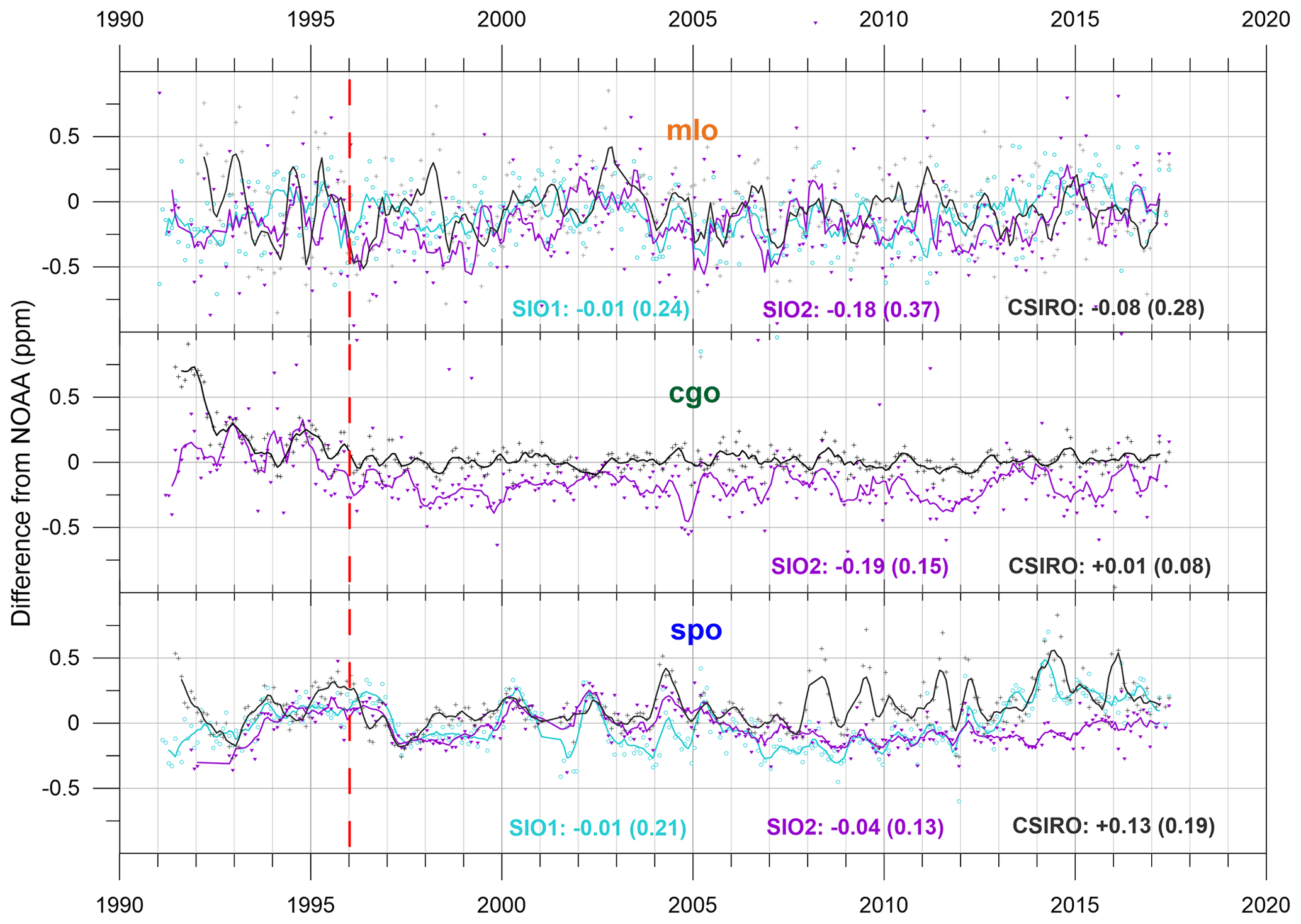
Figure 1 Monthly CO₂ differences (in ppm) from NOAA for sites mlo, cgo, and spo and networks SIO1, SIO2, and CSIRO. Five-month running means are highlighted. 1996–2016 mean and standard deviation (bracketed) values are included.

3 Network intercomparison

NOAA, which has the most extensive global network (and since 1996 has also operated the WMO CO₂ Central Calibration Laboratory) is selected as the reference for an initial inter-network comparison. For each of the three baseline sites, Fig. 1 shows systematic behaviour in the SIO1, SIO2, and CSIRO monthly CO₂ differences from NOAA. Five-month running means aid discussion. The CO₂ mixing ratios used here are referred to in the commonly used units of parts per million (ppm) rather than the more strictly correct term of μ mole of CO₂ per mole of dry air. Note that data independently flagged for sampling or measurement anomalies are rejected by individual laboratories prior to publication as monthly averages. Typically, a small number of gross outliers in individual flask data (e.g. in flask-pair differences) are also rejected prior to publication.

In Fig. 1, there is clear evidence of systematic differences in mean offsets, seasonality, and between sites within one network. In the context of interhemispheric exchange, the typical 0.5 ppm range of variation remains relatively small compared to the 7–10 ppm maximum CO₂ interhemispheric difference (IH ΔCO₂). Net IH exchange is proportional to IH partial pressure difference.

Between 1991 and 1993, there is a marked inconsistency between NOAA mlo–spo and mlo–cgo, particularly in seasonal amplitude; CSIRO has comparable measurements that are more consistent (Supplement S4). This is a reason for caution when interpreting the data in this period.

In the post-1996 statistics the SIO1 offsets from NOAA behave similarly for mlo and spo. This is not the case for SIO2, which has similar offsets at mlo (−0.18 ppm) and cgo (−0.19 ppm), but not at spo (−0.04 ppm), or for CSIRO (mlo: −0.08, cgo: +0.01, spo: +0.13 ppm).

CSIRO records at cgo exhibit the smallest offset and scatter relative to NOAA (±0.08 ppm) while SIO2 mlo data exhibit the largest scatter (±0.37 ppm).

Remnant seasonality is still evident in the CSIRO cgo differences from NOAA. While a small effect, the CSIRO GC/FID near-linear response for CO₂ means results are not so sensitive to differences between sample and reference CO₂. This advantage is reinforced in the CSIRO SH data since reference gases use recent SH baseline air. This is generally not the case for non-linear NDIR measurement and particularly in the NH if relatively short-lived reference gases sourced in the NH have a less-than-optimum match with ambient CO₂ from a site.

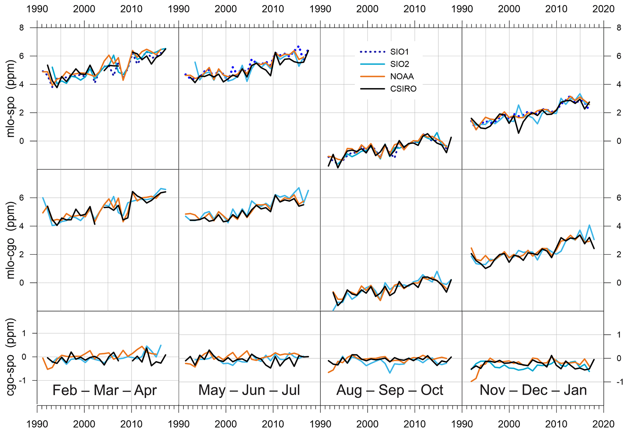
Figure 2 Three-month averaged CO₂ differences between sites for each of the four sampling networks: for years spanning 1990 to 2020.

While Fig. 1 reveals some un-resolved systematic differences between data sets, Fig. 2 emphasizes that they are generally small compared to the IH partial pressure differences that are a pre-requisite for IH net exchange. Data from each method are presented as 3-month seasonal averages in order to minimize potential influences related to network sample frequency (by ensuring an adequate number of individual flask samples per period). In addition, the particular 3-month seasonal selection distinguishes periods of distinct relatively stable partial pressure differences between hemispheres and the selected seasons also distinguish eddy and mean IH transport mechanisms (FF18).

Figure 2 demonstrates the considerable coherence between data sets.

• For the most part, and particularly in the August–October season when IH CO₂ difference (IH ΔCO₂) is at a minimum, there is a high level of consistency in the year-to-year variation in seasonal spatial differences from each network.

• There are relatively few examples of one record differing markedly from the others; when it occurs, it is often for reasons evident in Fig. 1. For example, in Fig. 2 NOAA cgo–spo appears low in 1992–1993; CSIRO mlo–spo shows negative outliers in May–July 2009 and November–January 2002, but not for mlo–cgo. SIO2 outliers in 2002 and 2006 exhibit similar characteristics; positive outliers, e.g. SIO2 from November to January 2016, suggest a cgo problem. In February–April 2005 NOAA data indicate a possible mlo problem; however, this is also when the “volatility” of the records (and in IH transport) is large, so it is conceivable that different flask sampling numbers and times could contribute to lower values by both SIO and CSIRO.

• The largest IH ΔCO₂ variability is recorded in February–April and in May–July, both seasons having near-equally large IH differences. The large seasonality in NH CO₂ is widely linked to the photosynthesis/respiration in NH forests. February–April is also when IH exchange by eddy processes is most influential (FF16), whereas mean transport via the Hadley circulation is the main dynamical influence in May–July (FF18).

Systematic differences due to sampling and measurement methodology can possibly arise from factors such as the linearity of instrument response, flask storage effects or undetected entrainment of laboratory air. Records with the sparsest sample density (e.g. at spo and particularly in CSIRO spo data) may be more susceptible to undetected anomalies. Closer inspection of individual flask metadata, or of the less extensive in situ monitoring, may resolve some of these infrequent anomalies, but for the present, composite averaging of the flask data is relied on to moderate their influence.

4 Composite records of baseline station spatial differences

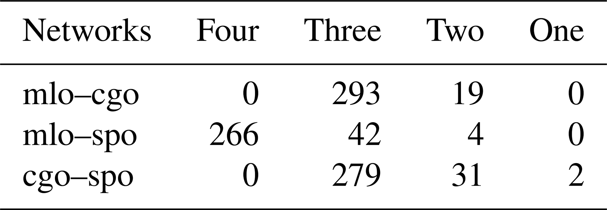
For each of mlo–cgo, mlo–spo, and cgo–spo monthly CO₂ differences, Table 1 shows the number of months between 1992 and 2017 contributing to a composite value, arranged in columns indicating the number of contributing networks; e.g. 266 of 31 months have four networks contributing to mlo–spo, while 279 months have three contributing networks at mlo–cgo.

The percentage of missing months for each network, and scatter in the composite differences for different historic periods, are tabulated in Supplement S1.

Table 1 Number of months of data available for composite differences at the baseline sites.

The monthly composite CO₂ differences are shown in Fig. 3 (and tabulated in Supplement S5). The small error bars represent the ensemble standard deviation (the one exception is for cgo–spo in February 2009, with only the NOAA network contributing. It is arbitrarily assigned 100 % uncertainty and appears as an outlier in Fig. 3c). The seasonality at mlo, generally attributed to the NH forest photosynthesis/respiration cycle, is the dominant variation in IH ΔCO₂. The composite uncertainties are small compared to seasonal amplitudes, especially for the IH differences. Average standard deviations of mlo–cgo, mlo–spo, and cgo–spo are 0.25, 0.23, and 0.16 ppm respectively. Systematic year-to-year variability is well defined and is reflected similarly in both IH records and is consistent with mlo driving most of the seasonal variation.

Variations that exceed the ensemble monthly standard deviations include the following.

• The overall increase in IH difference, generally attributed mainly to increasing NH fossil fuel CO₂ emissions, is indicated by a linear regression through the mlo–cgo values (with slope 0.056±0.021 ppm yr⁻¹; mlo–spo gives 0.062±0.021 ppm yr⁻¹). The slope of such regressions is much higher for the April–May data (0.087±0.011 ppm yr⁻¹) than for September–October data (0.049±0.011 ppm yr⁻¹).

• From 1992 to 2017, most minima occur in September; of 26 minima, 24 occur in September and 2 in October (1992 and 1995). Of the 26 maxima, 20 are in May, and 6 in April (1997, 1999, 2000, 2004, 2005, and 2016).

• Scatter in the amplitude of seasonal maxima (boreal winter/spring) is smaller before 1999. The step-like behaviour in April–May from 2009 to 2010 remains the major anomaly.

• In contrast, the minima (in boreal summer/autumn) exhibit greater scatter before 2011, replaced afterwards by a smooth decline to a marked 2016 minimum, then sudden reset in 2017.

• Unusually low boreal summer/autumn IH minima also occur in 1993–1994. Apart from being a period when measurement and calibration methods were consolidating (as discussed in the next section) the most significant volcanic influence (Pinatubo) is potentially an influence at this time.

A question arises as to how well mlo data represents the NH. Of more relevance to this study is how well the mlo samples represent air that is transferred into the Southern Hemisphere. Flask samples are collected at mlo above 3 km altitude in downslope winds, close to the upper troposphere regions where the IH transfer processes defined in FF18 occur (see Fig. 5 below), circumstances not shared by other NH surface monitoring sites.

Unlike in typical growth rate analyses, the peak and dip values are largely independent. This is visually explored in Fig. 3 using plotting software, with spline polylines linking peaks (solid) and dips (dashed) months of IH ΔCO₂. Trace gas mixing within extratropical (ET) hemispheres is typically estimated at 1–2 months or less, and interhemispheric exchange times are estimated at 6–12 months or more (e.g. Bowman and Cowan, 1997; Jacob, 1999). Monthly changes in the peak and dip IH ΔCO₂ largely reflect flux changes in or out of the extratropical northern troposphere close to that month. The following sections seek similarities with possible causal forcing processes.

5 Processes influencing CO₂ IH difference variations

Global carbon cycle models generally attribute short-term variations in atmospheric CO₂ to exchanges with the terrestrial biosphere (Le Quéré et al., 2018; Rödenbeck et al., 2018; Yue et al., 2017) and implicitly assume model atmospheric transport is correct on all time frames. While the models have demonstrated an impressive ability to predict mid-to-high-latitude CO₂ variations influenced by weather, it is less clear that short-term variations in IH exchange (of a magnitude sufficient to influence hemispheric growth rates) have been adequately captured.

5.1 Air–surface fluxes influencing IH ΔCO₂

The relative magnitude and timing of monthly variations of IH ΔCO₂ are compared to those in the terrestrial biosphere, wildfires, and fossil fuel (possible contributions from air–sea exchange are discussed below in relation to Fig. 8.)

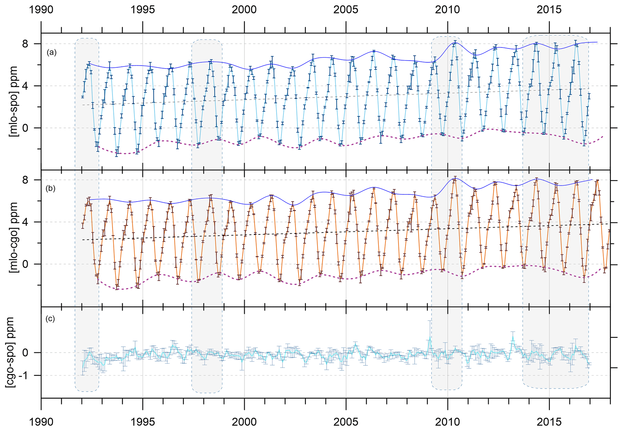
Figure 3 Composite station difference data showing the network ensemble average and standard deviation of monthly CO₂ for (a) mlo–spo, (b) mlo–cgo, and (c) cgo–spo (on a doubly expanded scale). Linear regressions through the IH records are black-dotted lines. Spline polylines visually link peaks (blue, solid) and dips (red, dotted) of the seasonal IH differences. Grey-shaded and rounded panels indicate El Niño periods with strongly anomalous equatorial zonal winds.

The primary determinant of the well-defined seasonality in IH ΔCO₂ in Fig. 3 is widely attributed to the temperature-moderated photosynthesis/respiration cycle of NH forests. Monthly dynamic vegetation model (DVM) estimates of terrestrial net biosphere production (NBP) in three latitude bands 90 to 30^∘ N, 30^∘ N to 30^∘ S, and 30 to 90^∘ S, over the 1992–2016 period are obtained using the Community Atmosphere Biosphere Land Exchange (CABLE) model (Kowalczyk et al., 2006; Haverd et al., 2018). In addition, ET NBP from an ensemble of 16 land surface models (shown in Fig. 2 of Bastos et al., 2018) are considered. Because of the small SH contribution, the ensemble ET values are most comparable to CABLE NH NBP. Note: We do not discuss air–surface fluxes derived from CO₂ data that are less spatially representative and/or rely on atmospheric transport modelling. The latter introduce additional model degrees of freedom and potentially overestimate terrestrial variability if the variability in atmospheric IH transport is not adequately captured.

NBP signs are reversed and are described as terrestrial-to-air carbon fluxes. Global wildfire emissions from the Global Fire Emissions Database (Randerson et al., 2018, GFED4.1) from 1997 to 2015 are classified as NH, EQ and EQ/SH. Seasonal anthropogenic emission anomalies are calculated as differences from the detrended 2000 to 2016 monthly data of Oda et al. (2018). For each data set, anomalies (in PgC month⁻¹) in seasonal behaviour for each latitude band were determined by subtracting the mean seasonality from the monthly values.

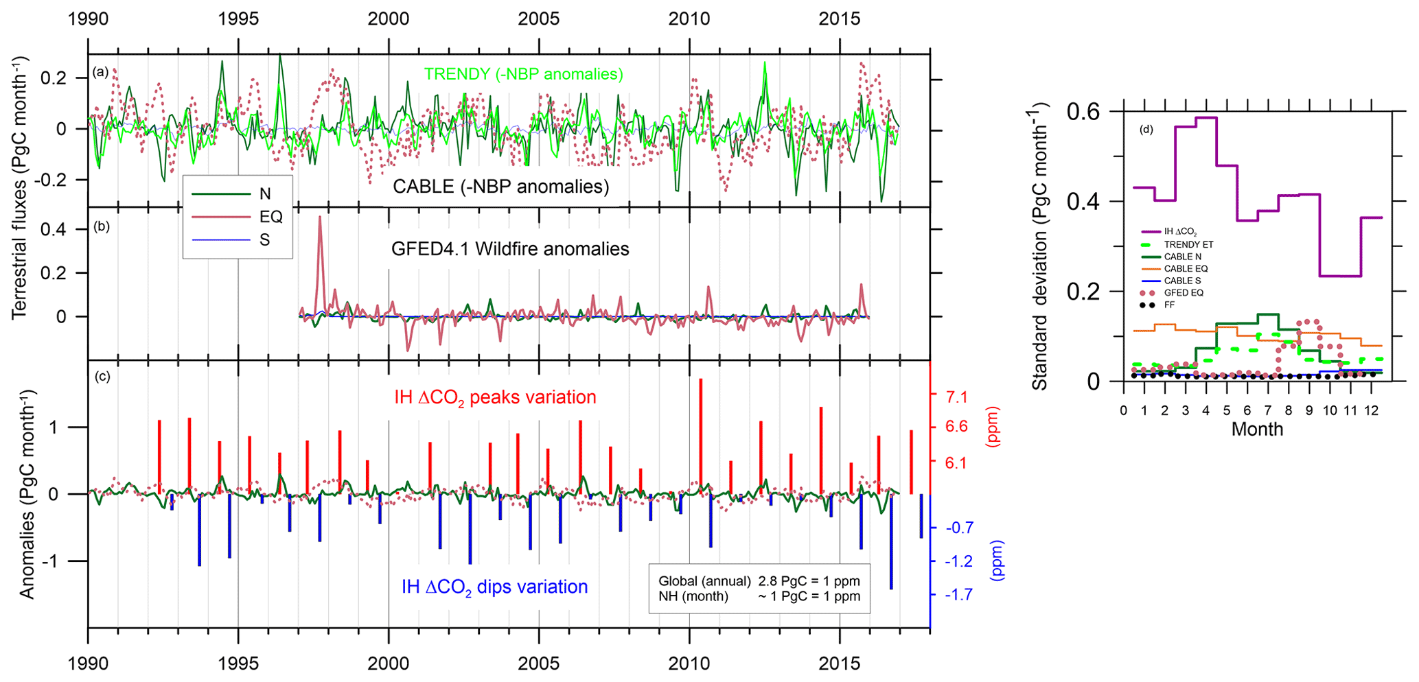
Figure 4 Comparison of the timing and amplitude of terrestrial emission anomalies (i.e. mean seasonality subtracted) with variations of the peaks and dips in Fig. 3. (a) shows seasonal anomalies in CABLE emissions (dark green) and in 16-DGVM TRENDY ET emissions (Bastos et al., 2018; light green) and (b) shows GFED4.1 wildfire seasonal anomalies, for NH (green), EQ (pink), and SH (blue, SH/EQ for GFED4.1). In (c) the largest anomalies (CABLE NH, CABLE EQ, and GFED4.1 EQ) on the left axis are compared to the ppm variation in peaks (red) and dips (blue) on separate right axes. The axes scaling equates 1 PgC with 1 ppm (see text). To highlight seasonal differences, (d) shows the standard deviation in the seasonal anomalies for each month, including those in anthropogenic emissions (Oda et al., 2018).

The major seasonal anomalies in NBP and wildfire emissions that potentially influence IH ΔCO₂ are shown in Fig. 4a and b. The largest anomalous surface-to-air flux is the extreme equatorial emission anomaly from equatorial wildfire in late 1997 (∼0.9 PgC over 3 months); it is not associated with unusual behaviour in the IH ΔCO₂ records.

Despite mixing of CO₂ within the ET Northern Hemisphere being as rapid as 1–2 weeks (Jacob, 1999) compared to IH exchange times of greater than 6 months (Bowman and Cowan, 1997), we see strong correlations with transport for unlagged 3-month averages. And since IH ΔCO₂ peaks re-occur within 1 month of the same time each year, close correspondence in timing of terrestrial anomalies and the IH ΔCO₂ peaks would be expected if NH terrestrial exchange was the main determinant. This is not evident in Fig. 4. More importantly, the amplitude range of terrestrial anomalies appears to be far too small to account for the magnitude of the changes in the peaks and dips of IH ΔCO₂.

Over the last 25 years the annual relationship between global (mainly NH) fossil fuel combustion emissions and IH ΔCO₂ has been 2.8 PgC ppm⁻¹ (equivalent to the 0.36 ppm (PgC)⁻¹ used by FF18). This is applicable when northern fossil fuel emissions effectively mix globally. The volume of the troposphere north of Mauna Loa is around 33 % of the global troposphere, so that on the shorter time frame of within-hemisphere mixing, only ∼0.92 PgC is required to change the NH background CO₂ by 1 ppm. In Fig. 4c we round this to 1 PgC =1 ppm for simplicity.

The variability in the air–surface fluxes, relative to that in IH ΔCO₂, is displayed in Fig. 4d, which plots the standard deviations of residuals from the mean seasonality, for each month over the available record. As for the peaks and dips, we assume a 1:1 relationship between ppm and PgC month⁻¹ in IH ΔCO₂. The main variation in IH ΔCO₂ occurs in March–April, when variability in surface–air fluxes is small but variability in eddy IH exchange is large (see below). A second peak in IH ΔCO₂ standard deviation occurs August–September, around the time of the dips (but also when equatorial wildfires are more active suggesting a possible contribution from the equatorial emissions at this time).

Accepting the precision and near-hemispheric spatial representation of the composite IH ΔCO₂ records, these inconsistences with surface emissions in both timing and magnitude suggest that there are other short-term influences on IH ΔCO₂ of greater magnitude than air–surface exchange.

5.2 Wind indices reflecting CO₂ IH transport

In contrast to the case for air–surface exchanges, there are a number of prominent features in the composite IH ΔCO₂ records that are shared with behaviour in the dynamical indices of FF18. Interhemispheric exchange of CO₂ occurs mainly by eddy processes in the boreal winter–spring and by mean convection and advection associated with the Hadley circulation in the boreal summer–autumn (FF18 and references therein). FF18 developed wind indices that characterize both types of IH transport based on reanalysis data sets focussing on the National Center for Environmental Prediction (NCEP) and National Center for Atmospheric Research (NCAR) reanalysis (NRR) data (Kalnay et al., 1996). Eddy transport is described by u_duct, the average 300 hPa zonal velocity in the Pacific westerly duct region (Frederiksen and Webster, 1988) of 5^∘ N to 5^∘ S, 140 to 170^∘ W (FF16, FF18). Here we use that index and two of the four indices for mean transport introduced in FF18. These are ω_P, the average 300 hPa vertical velocity in pressure coordinates in the region 10 to 15^∘ N, 120 to 240^∘ E, and v_P the average 200 hPa meridional velocity in the region 5 to 10^∘ N, 120 to 240^∘ E. Figure 5 provides a schematic of the geographical location of regions used by FF18, and time series of the monthly values of wind indices are shown in Fig. 6.

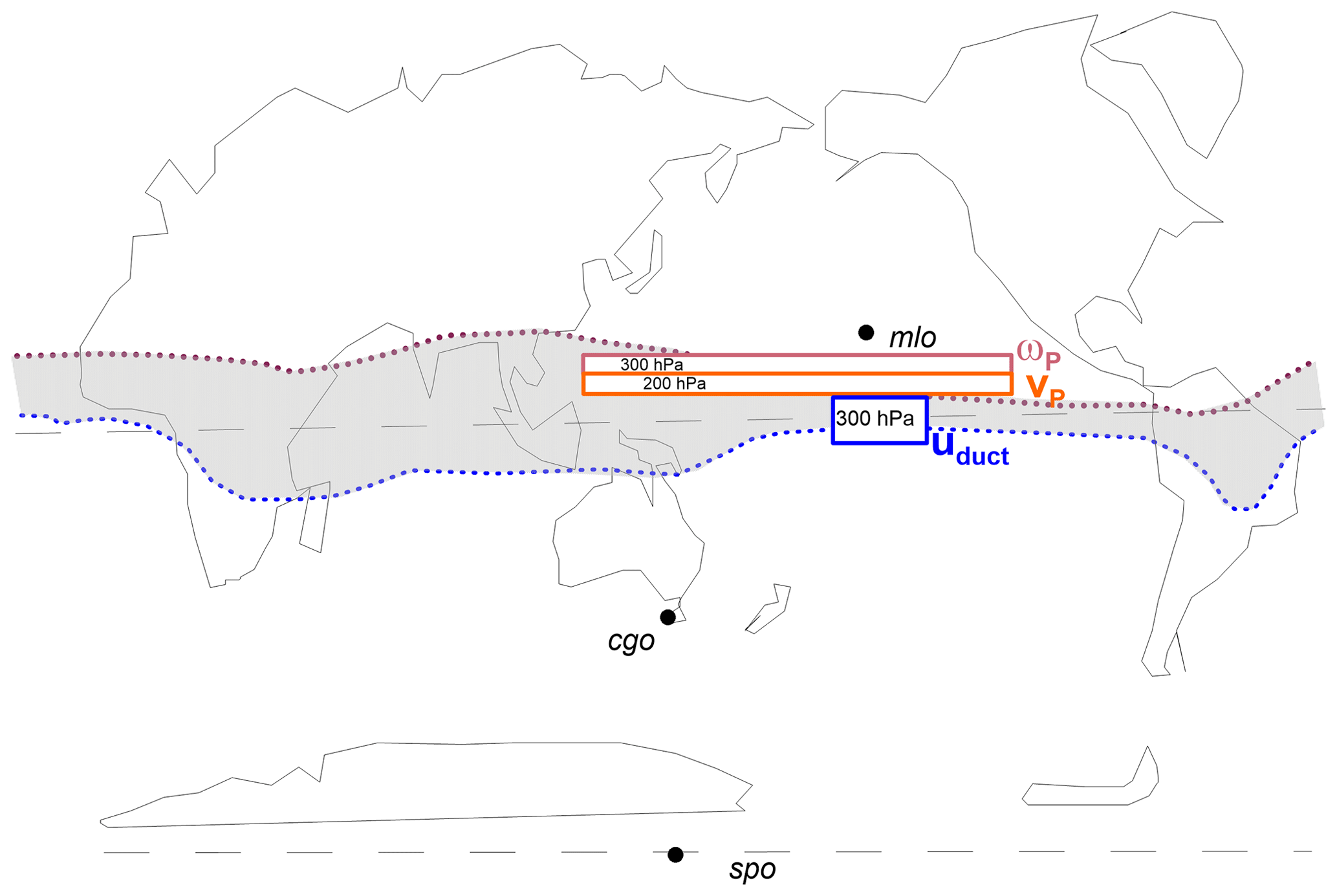
Figure 5 Schematic of the boundaries and altitudes of regions used in FF18 to define wind indices that describe eddy IH transfer (u_duct, westerlies positive) and mean transfer (uplift, negative ω_P) and north-to-south transfer (negative v_P). The shaded area brackets the austral summer extent of the Intertropical Convergence Zone in the south (blue dash) and boreal summer extent in the north (red dash).

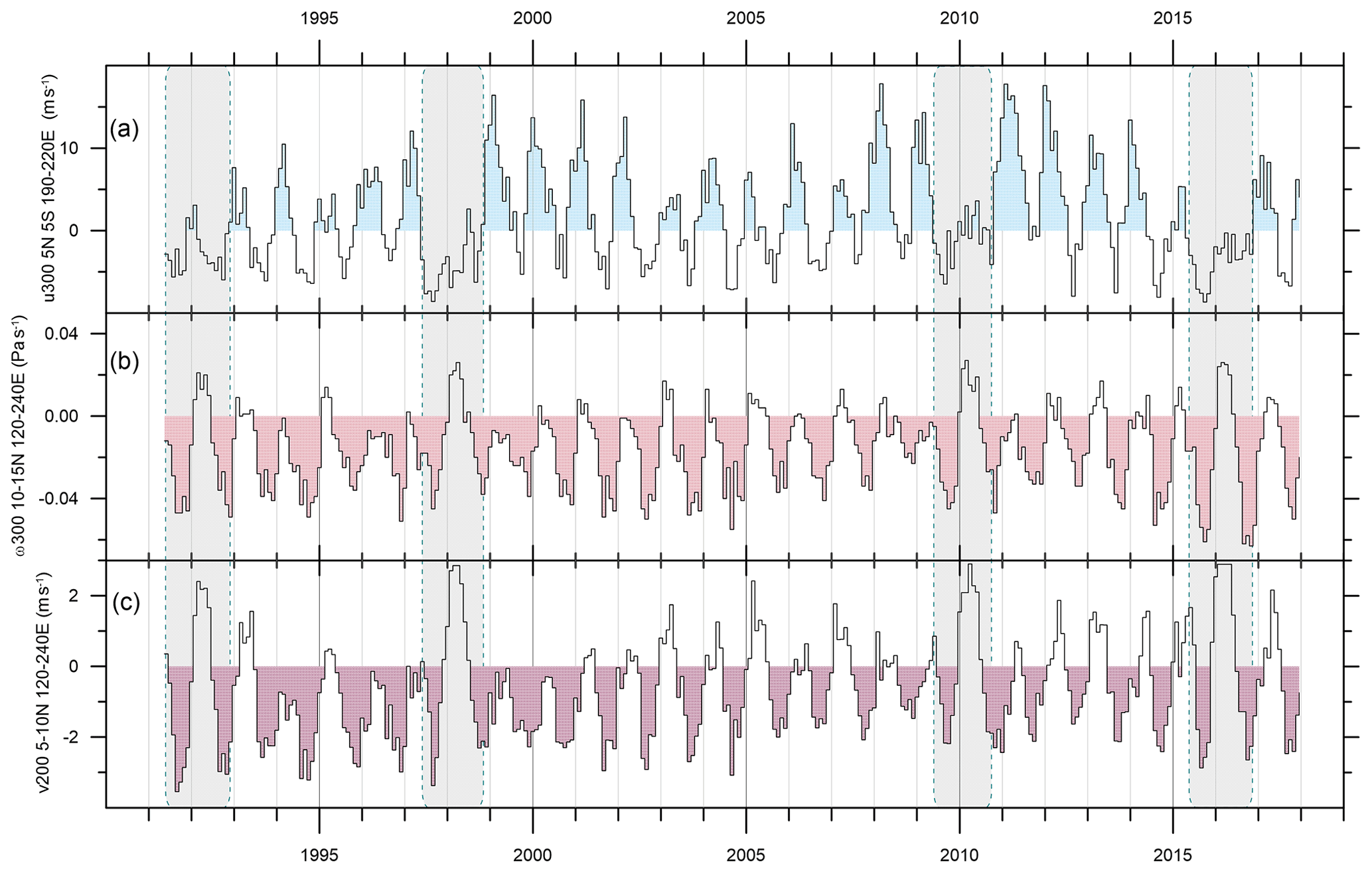
Figure 6 Monthly values of (a) u_duct, (b) ω_P, and (c) v_P. The shading to zero indicates months of enhanced transport which act to reduce the IH ΔCO₂. Anomalous dynamical periods are highlighted with grey-shaded rectangles.

The top panel in Fig. 6a shows a 3-decade time series of the u_duct index which characterizes cross-equatorial Rossby wave dispersion, Rossby wave breaking, and corresponding increases in transient kinetic energy and eddy transport in the near-equatorial upper troposphere (Webster and Holton, 1982, Frederiksen and Webster, 1988, Ortega et al., 2018). The large-scale Rossby waves are generated by thermal anomalies and topographic features including the Himalayan mountains from which they propagate south-eastward and are able to penetrate into the SH when u_duct is positive, corresponding to an open Pacific westerly duct.

The ω_P and v_P indices in Fig. 6b and c describe the strength of the mean transport by the Hadley cell in the Pacific region with negative ω_P corresponding to uplift and negative v_P to north-to-south transport.

Net interhemispheric trace gas exchange requires a partial pressure difference between hemispheres. For CO₂ the average seasonal cycle of a 25-year mean partial pressure difference, represented here by monthly baseline mlo–cgo, is shown in Fig. 7a (mlo–spo is not shown here since, reflecting on data quality, it is effectively identical).

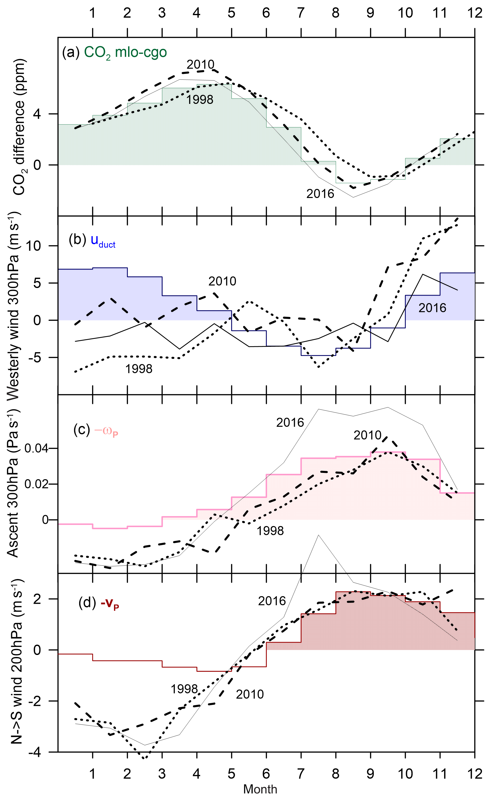
Figure 7 The monthly averages of dynamical factors governing CO₂ IH exchange over the last 25 years. (a) Detrended CO₂ partial pressure differences mlo–cgo (green), (b) Pacific eddy transport index u_duct (dark blue), (c) Pacific Hadley transport indicated by uplift at 10–15^∘ N (-ω_P, light red), and (d) north-to-south transport (-v_P, dark red). On average, coincidence of shading in wind indices and shaded months of IH ΔCO₂ is a precondition for increased IH mixing (reduced IH gradient). The more anomalous transport years, 1998 (dots), 2010 (dashes), and 2016 (black line) are shown for each wind index, and for mlo–cgo IH ΔCO₂.

The positive mean IH ΔCO₂ is largely due to fossil fuel emissions. Months of positive (north–south) IH difference are shaded green and only in September–October is there a small reverse gradient. Transport of CO₂ from the Northern to the Southern Hemisphere occurs when green-shaded areas in Fig. 7a coincide (on average) with blue-shaded areas (Fig. 7b, via eddy transfer with index u_duct) or with red-shaded areas (Fig. 7c and d, via mean transport with indices ω_P and v_P).

Figure 7 also demonstrates that differences from the long-term mean in transport indices (average for each month) vary between the significant El Niño events in 1998, 2010, and 2016:

• In 2010, the IH ΔCO₂ exceeds the average between February and July (Fig. 7a) with reduced eddy transfer between February and April, associated with lower that average u_duct (Fig. 7b). Further, between June and September, there is weaker ascent (Fig. 7c) and north-to-south upper tropospheric wind (Fig. 7d) in the key regions defining ω_P and v_P. As noted in FF18, the IH ΔCO₂ eddy and mean transports reinforce to contribute to the unprecedented 2009–2010 step in IH ΔCO₂.

• In 2016, the IH ΔCO₂ is larger than average between February and June and smaller than average between July and October (Fig. 7a). These results are again consistent with the behaviour of the dynamical indices. There is reduced IH ΔCO₂ eddy transfer in the first half of the year (Fig. 7b) but very strong mean transport in the second half of the year (Fig. 7c and d) that accounts for the annual IH ΔCO₂, as noted in FF18.

• In 1998, the IH ΔCO₂ exceeds the average from May to December and is close to the mean annual cycle for the rest of the year. We note from Fig. 7 that the annual increase in IH ΔCO₂, also shown in Fig. 2 of FF18, is largely induced by the June–August mean Hadley circulation.

• It is suggestive that the relative variation in IH ΔCO₂ February–May for the three big El Niño years matches that in u_duct, however it is puzzling that the largest u_duct anomaly, in 1998, is when IH ΔCO₂ is closest to the mean behaviour. The fact that the mean transport indices at this time of year are also consistently well below their long-term average is also of note, since with u_duct close to zero and -ω_P, -v_P indicating descent and south-to-north meridional winds, there is no obvious mechanism for IH exchange in this season. Yet, over the 25 years, correlation of the April–May IH ΔCO₂ peaks with -ω_P-v_P is significant, r≈ 0.4. One possible explanation for these behaviours in the early part of the boreal winter/austral summer may be found in changes in the volume of the well-mixed portion of the Northern Hemisphere (see Discussion, Sect. 7).

Different responses of IH ΔCO₂ to wind indices at different ENSO events, and from non-ENSO periods, are discussed in Sect. 7.

As an aside, we also include a similar plot for the average SH cgo–spo differences in Fig. 8. Despite some concerns about artefacts in spo data (e.g. due to long flask-air storage times), all networks indicate that on average spo baseline CO₂ exceeds that at cgo in the austral summer months. The minimum cgo–spo appears to precede inversion estimates of Southern Ocean CO₂ uptake south of 30^∘ S (Lenton et al., 2013). High-precision continuous CO₂ monitoring across the Southern Ocean (Stavert et al., 2019; Ann Stavert, personal communication, 2018) confirm small and relatively smooth seasonal variation. The earlier November–December minimum in the CO₂ difference coincides with a seasonal dip in fossil fuel emissions (Oda et al., 2018) perhaps indicating an alternative explanation.

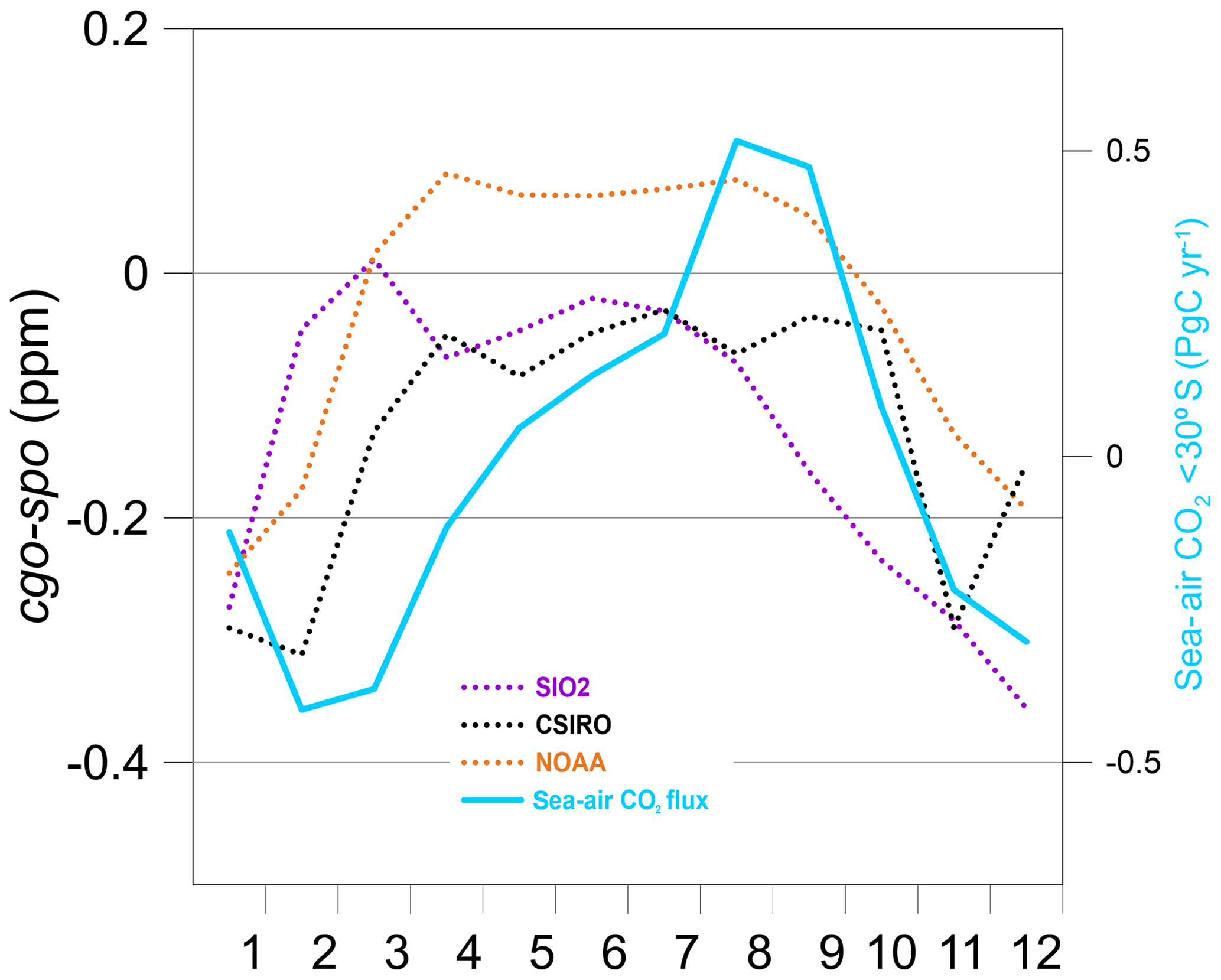
Figure 8 Composite 25-year average of monthly baseline cgo–spo CO₂ (dark blue). Individual network values are shown in orange (NOAA), dark blue (SIO2), and CSIRO (black). Estimates of sea–air CO₂ flux seasonality are shown in light blue.

6 Year-to-year variation in the composite records

The annual net impacts of the various potential influences on site IH ΔCO₂ (when typical terrestrial biosphere seasonal variations are balanced) appear in Fig. 9. Uncertainty in annual values obtained from combining composite standard deviations of normalized monthly values for the cgo case, averaging ±0.08 ppm, compares to $\sim \pm \mathrm{0.3}$ ppm variation in the detrended annual record.

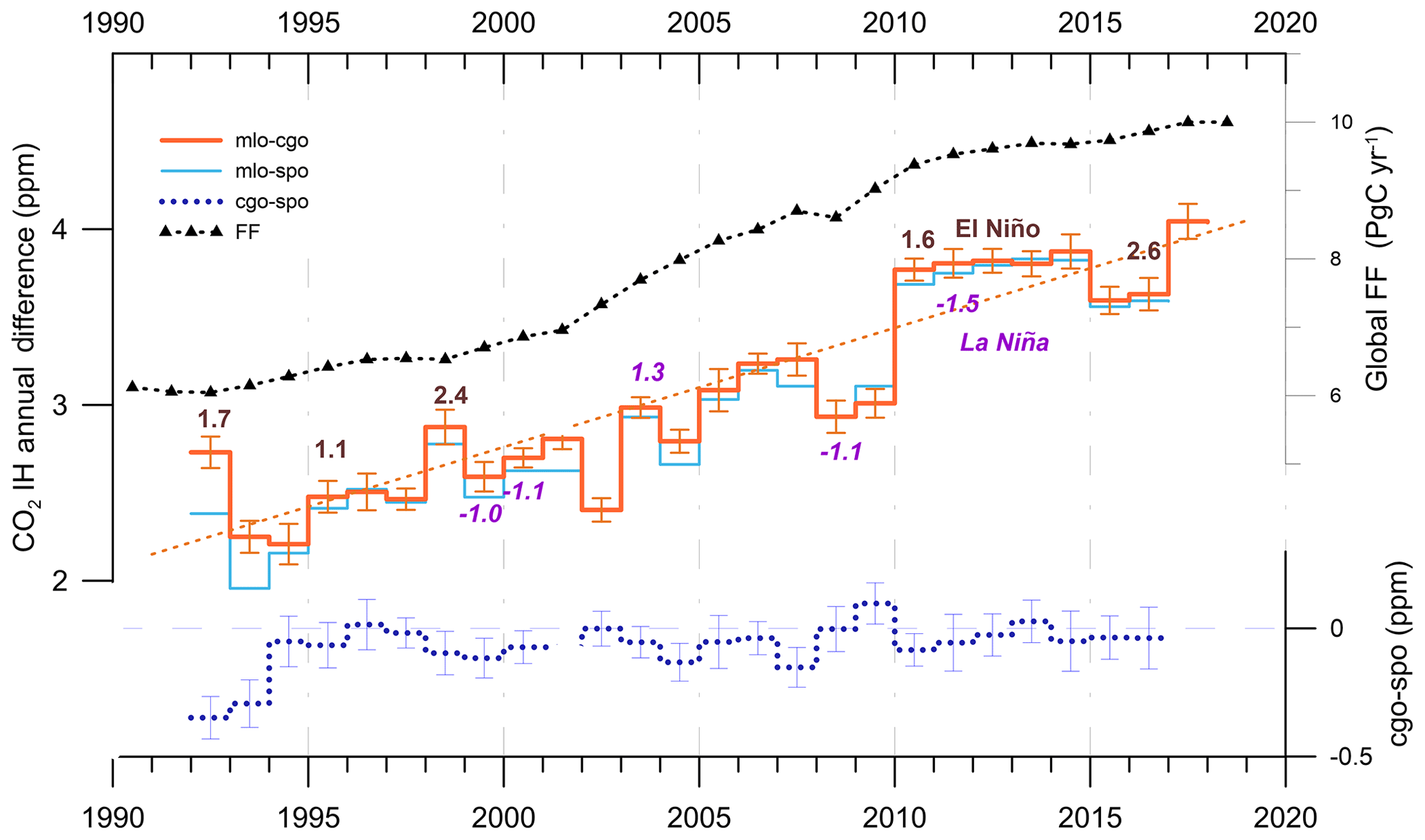
Figure 9 Annual changes in the baseline CO₂ difference between sites. Interhemispheric differences mlo–cgo (orange, with dashed linear regression) and mlo–spo (light blue) are plotted on the left axis. The peak magnitudes of strong El Niños (brown, ONI index > 1) and strong La Niñas (purple, ONI index < −1) are indicated. The cgo–spo annual differences are plotted on a doubled right-hand scale. Annual fossil fuel emissions from FF18, are shown on the top right axis.

Working through Fig. 9 from the left in order to highlight other systematic features:

• Except for 2016, every major El Niño event (as indicated by the magnitude of the peak Oceanic Niño Index, when ONI > 1) corresponds to a transition from a low to high IH difference. The ONI is a 3-month running mean of the Nino3.4 index; similar treatment of Nino3 yields correlation coefficients with Nino3.4 of 0.94 for both the annual maxima and minima from 1992 to 2018. However, the CO₂ response is not proportional to ONI, e.g. when comparing 2009–2010 to 1997–1998, or most noticeably to 2015–2016 (the strongest ONI but the smallest IH ΔCO₂ step).

• There is remarkable stability in IH ΔCO₂ from 2010 to 2014 (despite the strong La Niña in 2011). After 2010, there are no significantly positive ONI anomalies (El Niños), and the 5-year increase of ∼0.1 ppm is lower than that generally attributed to the increasing mean fossil fuel emissions (the 2010–2014 change in FF is 0.73 ppm yr⁻¹, which at 0.36 ppm (PgC)⁻¹ would result in a 0.26 ppm increase). The FF with this scaling is shown at the top. There is markedly less variability (the composite standard deviation of de-trended annual means is 0.04 ppm) than any equivalent period over the previous 16 years (0.31 ppm).

• The 2009–2010 year-to-year change of ∼0.8 ppm (addressed in FF16 using CSIRO data only) remains the major year-to-year change in the annual records. The current composite data confirm the general FF16 conclusion.

• The linear regression through the 25-year mlo–cgo annual data gives a slope of 0.067±0.006 ppm yr⁻¹ compared to that through monthly values of 0.56±0.021 ppm yr⁻¹ in Fig. 3, or through the peaks of 0.087±0.011 ppm yr⁻¹ or the dips of 0.049±0.011 ppm yr⁻¹. We interpret this as indicating the combined long-term influence of both eddy and mean transport on the annual mean IH ΔCO₂.

• In 2017, the IH difference is close to the 3-decade trend, with the duct open and Hadley strength returning to be close to its long-term mean.

7 Discussion

The composite monthly IH differences reveal variation from monthly to decadal timescales that exceed measurement and sampling error (as indicated by the composite standard deviations) thus requiring biogeochemical explanation. This discussion focusses on the potential of IH transport measured by wind indices to explain major features in IH ΔCO₂ variation, with emphasis on periods and events when they are likely to be the dominant influence on IH ΔCO₂. It complements the more general statistical analyses in FF18. In Fig. 6, decreasing u_duct acts to lessen eddy IH exchange and increase IH ΔCO₂, while the increasing Hadley circulation (decreasing v_P and ω_P) decreases IH ΔCO₂.

The fact that the magnitude of IH ΔCO₂ response varies greatly between the 1998, 2010, and 2016 El Niño events (with little or no eddy transfer occurring in boreal winter/spring in these years) is consistent with a quasi-decadal variation in the negative excursions of v_P and ω_P in Fig. 6 (most obvious in ω_P). In 1998 and 2010, the Hadley boreal summer/autumn indices are closer to zero, while 2016 registers an unprecedented negative excursion.

The complication of IH ΔCO₂ variations in the boreal winter/austral summer when u_duct, ω_p and v_P indices indicate that little or no IH exchange occurs (and u_duct closure tends to increase mlo CO₂) is at a time when the north-to-south seasonal variation in the Intertropical Convergence Zone (ITCZ) is near maximum. If NH peak terrestrial emissions (biospheric and industrial) at that time are diluted into a larger volume of well-mixed NH air, it could offset the mlo CO₂ increase anticipated from u_duct closure. This volume effect is likely to be a second-order effect in non-El Niño years.

NH terrestrial biosphere emission anomalies in the 2010–2014 period (Fig. 4) are more variable than those in 2000–2005, the opposite of the relative behaviour in IH ΔCO₂ variability in Fig. 9. These emissions are relatively small, and frequently occur after the larger IH ΔCO₂ anomalies, all inconsistent with a significant contribution to the composite IH differences; thus, they are considered second order. The small 2010–2014 trend (∼0.1 ppm compared to 0.26 ppm expected from fossil fuel emissions), and the steadily decreasing westerly wind strength in u_duct over the period, should increase IH ΔCO₂ over the fossil fuel trend (FF16). The flattening trend is consistent with the IH ΔCO₂ flux due to IH mixing by the Hadley process overwhelming the increases expected from fossil fuel combustion and from decreasing u_duct strength. There is a linear relationship between u_duct and equatorial upper troposphere transient kinetic energy shown in Fig. 6 of Frederiksen and Webster (1988) and discussed in FF16 and FF18. Note that in Fig. 6, there is no precedent for similar sustained opposing behaviour in the two modes of IH transfer. The trend and lack of scatter in 2010–2014 IH ΔCO₂ can be understood by the IH ΔCO₂ fluxes being significantly larger than air–surface exchanges at the time.

The magnitude of the IH flux anomalies of up to ∼2 PgC month⁻¹ exceed known air–surface fluxes in the NH and are of a sufficient magnitude to significantly influence NH CO₂ growth rate variability. With increasing fossil fuel fluxes, the role of IH exchange on IH ΔCO₂, and NH CO₂ growth, is expected to become increasingly important.

The previous inability of carbon cycle models to simulate the 2009–2010 step (FF16, Supplement) suggests that there is inadequate parameterization of IH ΔCO₂ transfer, particularly by eddy exchange, in some global carbon cycle models. If this is the case, then studies that interpret CO₂ behaviour during ENSO events as a guide to terrestrial biosphere responses to climate (e.g. Rödenbeck et al., 2018) will also be compromised. The ability to simulate the identified features of the composite IH ΔCO₂ (within the standard deviations) would provide convincing independent confirmation of atmospheric transport implementation.

8 Conclusions

Over the last 25 years there has been a high degree of agreement in the measurement of monthly spatial differences in background CO₂ levels by three measurement laboratories using four different sampling methodologies and sampling frequencies. Geographic isolation of sample collection sites and consistent sophisticated background selection over the 25 years, as well as coincident monitoring of a wide range of atmospheric species, excludes local and regional influence on CO₂ at mlo, spo, and cgo to an extent not generally available at other surface monitoring sites.

The temporal variation in the composite IH ΔCO₂ exhibit several systematic features on monthly to multi-year time frames that are not reflected in independent evidence of air–surface exchange but do correspond to features in dynamical indices selected to represent both eddy and mean IH exchange. The comparisons in this paper imply a major role for IH exchange of CO₂ in NH growth rate variations.

The evidence for a significant influence of atmospheric dynamics on the CO₂ IH gradient has relevance for global carbon cycle studies. It implies that both eddy and mean transport processes, and volume effects, need to be specifically included in transport model simulations, since the balance between the two is constantly changing, particularly in El Niño periods when eddy transport is reduced. It also means that El Niño events may be a poor predictor of the carbon cycle behaviour in non-ENSO years.

Global carbon cycle model simulations should be able to reproduce the major features identified here in the composite IH records if the re-analyses transport is correctly implemented. In attempting to simulate the composite differences, one complication is model selection of a baseline that matches the flask sampling criteria. While monthly baseline averages appear to succeed in this respect, a more comprehensive treatment (outside the scope of this study) based on individual flask measurements rather than monthly averages, and on other trace gas observations (FF16, FF18), and in particular radon (Chambers et al., 2016), could possibly improve this process.