the Creative Commons Attribution 4.0 License.
the Creative Commons Attribution 4.0 License.
 | 28 Nov 2019
Importance of dry deposition parameterization choice in global simulations of surface ozone
Anthony Y. H. Wong
Amos P. K. Tai
Sam J. Silva
Dry deposition is a major sink of tropospheric ozone. Increasing evidence has shown that ozone dry deposition actively links meteorology and hydrology with ozone air quality. However, there is little systematic investigation on the performance of different ozone dry deposition parameterizations at the global scale and how parameterization choice can impact surface ozone simulations. Here, we present the results of the first global, multidecadal modelling and evaluation of ozone dry deposition velocity (vd) using multiple ozone dry deposition parameterizations. We model ozone dry deposition velocities over 1982–2011 using four ozone dry deposition parameterizations that are representative of current approaches in global ozone dry deposition modelling. We use consistent assimilated meteorology, land cover, and satellite-derived leaf area index (LAI) across all four, such that the differences in simulated vd are entirely due to differences in deposition model structures or assumptions about how land types are treated in each. In addition, we use the surface ozone sensitivity to vd predicted by a chemical transport model to estimate the impact of mean and variability of ozone dry deposition velocity on surface ozone. Our estimated vd values from four different parameterizations are evaluated against field observations, and while performance varies considerably by land cover types, our results suggest that none of the parameterizations are universally better than the others. Discrepancy in simulated mean vd among the parameterizations is estimated to cause 2 to 5 ppbv of discrepancy in surface ozone in the Northern Hemisphere (NH) and up to 8 ppbv in tropical rainforests in July, and up to 8 ppbv in tropical rainforests and seasonally dry tropical forests in Indochina in December. Parameterization-specific biases based on individual land cover type and hydroclimate are found to be the two main drivers of such discrepancies. We find statistically significant trends in the multiannual time series of simulated July daytime vd in all parameterizations, driven by warming and drying (southern Amazonia, southern African savannah, and Mongolia) or greening (high latitudes). The trend in July daytime vd is estimated to be 1 % yr−1 and leads to up to 3 ppbv of surface ozone changes over 1982–2011. The interannual coefficient of variation (CV) of July daytime mean vd in NH is found to be 5 %–15 %, with spatial distribution that varies with the dry deposition parameterization. Our sensitivity simulations suggest this can contribute between 0.5 to 2 ppbv to interannual variability (IAV) in surface ozone, but all models tend to underestimate interannual CV when compared to long-term ozone flux observations. We also find that IAV in some dry deposition parameterizations is more sensitive to LAI, while in others it is more sensitive to climate. Comparisons with other published estimates of the IAV of background ozone confirm that ozone dry deposition can be an important part of natural surface ozone variability. Our results demonstrate the importance of ozone dry deposition parameterization choice on surface ozone modelling and the impact of IAV of vd on surface ozone, thus making a strong case for further measurement, evaluation, and model–data integration of ozone dry deposition on different spatiotemporal scales.
- Article
(7944 KB) - Full-text XML
-
Supplement
(842 KB) - BibTeX
- EndNote


Surface ozone (O3) is one of the major air pollutants that poses serious threats to human health (Jerrett et al., 2009) and plant productivity (Ainsworth et al., 2012; Reich, 1987; Wittig et al., 2007). Ozone exerts additional pressure on global food security and public health by damaging agricultural ecosystems and reducing crop yields (Avnery et al., 2011; McGrath et al., 2015; Tai et al., 2014). Dry deposition, by which atmospheric constituents are removed from the atmosphere and transferred to the Earth's surface through turbulent transport or gravitational settling, is the second-largest and terminal sink of tropospheric O3 (Wild, 2007). Terrestrial ecosystems are particularly efficient at removing O3 via dry deposition through stomatal uptake and other non-stomatal pathways (Wesely and Hicks, 2000) (e.g. cuticle, soil, reaction with biogenic volatile organic compounds (BVOCs); Fares et al., 2010; Wolfe et al., 2011). Meanwhile, stomatal uptake of O3 inflicts damage on plants by initiating reactions that impair their photosynthetic and stomatal regulatory capacity (Hoshika et al., 2014; Lombardozzi et al., 2012; Reich, 1987). Widespread plant damage has the potential to alter the global water cycle (Lombardozzi et al., 2015) and suppress the land carbon sink (Sitch et al., 2007), as well as generate a cascade of feedbacks that affect atmospheric composition including ozone itself (Sadiq et al., 2017; Zhou et al., 2018). Ozone dry deposition is therefore key in understanding how meteorology (Kavassalis and Murphy, 2017), climate, and land cover change (Fu and Tai, 2015; Ganzeveld et al., 2010; Geddes et al., 2016; Heald and Geddes, 2016; Sadiq et al., 2017; Sanderson et al., 2007; Young et al., 2013) can affect air quality and atmospheric chemistry at large.
Analogous to other surface–atmosphere exchange processes (e.g. sensible and latent heat flux), O3 dry deposition flux () is often expressed as the product of ambient O3 concentrations at the surface ([O3]) and a transfer coefficient (dry deposition velocity, vd) that describes the efficiency of transport (and removal) to the surface from the measurement height:
Also analogous to other surface fluxes, , [O3], and hence vd, can be directly measured by the eddy covariance (EC) method (e.g. Fares et al., 2014; Gerosa et al., 2005; Lamaud et al., 2002; Munger et al., 1996; Rannik et al., 2012) with random uncertainty of about 20 % (Keronen et al., 2003; Muller et al., 2010). Apart from EC, and vd can also be estimated from the vertical profile of O3 by exploiting flux–gradient relationship (Foken, 2006) (termed the gradient method, GM) (e.g. Gerosa et al., 2017; Wu et al., 2015, 2016). A recent study (Silva and Heald, 2018) complied 75 sets of ozone deposition measurement from the EC and GM across different seasons and land cover types over the past 30 years.
At the site level, ozone dry deposition over various terrestrial ecosystems can be simulated comprehensively by 1-D chemical transport models (Ashworth et al., 2015; Wolfe et al., 2011; Zhou et al., 2017), which are able to simulate the effects of vertical gradients inside the canopy environment, and gas-phase reaction with BVOCs in addition to surface sinks. Regional and global models, which lack the fine-scale information (e.g. vertical structure of canopy, in-canopy BVOC emissions) and horizontal resolution for resolving the plant canopy in such detail, instead represent plant canopy foliage as one to two big leaves, and vd is parameterized as a network of resistance, which accounts for the effects of turbulent mixing via aerodynamic (Ra), molecular diffusion via quasi-laminar sublayer resistance (Rb), and surface sinks via surface resistance (Rc):
A diverse set of parameterizations of ozone dry deposition is available and used in different models and monitoring networks. Examples include the Wesely parameterization (1989) and modified versions of it (e.g. Wang et al., 1998), the Zhang et al. (2003) parameterization (Zhang et al., 2003), the Deposition of O3 for Stomatal Exchange model (Emberson et al., 2000; Simpson et al., 2012), and the Clean Air Status and Trends Network (CASTNET) deposition estimates (Meyers et al., 1998). The calculation of Ra (mostly based on Monin–Obukhov similarity theory) and Rb across these parameterizations often follow a standard formulation from micrometeorology (Foken, 2006; Wesely and Hicks, 1977, 2000; Wu et al., 2011) and thus does not vary significantly. The main difference between the ozone dry deposition parameterizations lies on the surface resistance, Rc. This resistance includes stomatal resistance (Rs), which can be computed by a Jarvis-type multiplicative algorithm (Jarvis, 1976) where Rs is the product of its minimum value and a series of response functions to individual environmental conditions. Such conditions typically include air temperature (T), photosynthetically available radiation (PAR), vapour pressure deficit (VPD), and soil moisture (θ), with varying complexity and functional forms.
Such formalism is empirical in nature and does not adequately represent the underlying ecophysiological processes affecting Rs (e.g. temperature acclimation). An advancement of these efforts includes harmonizing Rs with that computed by land surface models (Ran et al., 2017a; Val Martin et al., 2014), which calculate Rs by coupled photosynthesis–stomatal conductance (An–gs) models (Ball et al., 1987; Collatz et al., 1991, 1992). Such coupling should theoretically give a more realistic account of ecophysiological controls on Rs. Indeed, it has been shown that the above approach may better simulate vd than the multiplicative algorithms that only consider the effects of T and PAR (Val Martin et al., 2014; Wu et al., 2011).
The non-stomatal part of Rc often consists of cuticular (Rcut), ground (Rg), and other miscellaneous types of resistance (e.g. lower canopy resistance (Rlc) in Wesely, 1989). Due to very limited measurements and mechanistic understanding towards non-stomatal deposition, non-stomatal resistance is often constant (e.g. Rg) or simply scaled with leaf area index (LAI) (e.g. Rcut) (Simpson et al., 2012; Wang et al., 1998; Wesely, 1989), while some of the parameterizations (Zhang et al., 2003; Zhou et al., 2017) incorporate the observation of enhanced cuticular O3 uptake under leaf surface wetness (Altimir et al., 2006; Potier et al., 2015, 2017; Sun et al., 2016).
Furthermore, terrestrial atmosphere–biosphere exchange is also directly affected by CO2, as CO2 can drive increases in LAI (Zhu et al., 2016) while inhibiting gs (Ainsworth and Rogers, 2007). These can have important implications on vd, as shown by Sanderson et al. (2007), where doubling current CO2 level reduces gs by 0.5–2.0 mm s−1, and by Wu et al. (2012) where vd increases substantially due to CO2 fertilization at 2100. Observations from the Free Air CO2 Enrichment (FACE) experiments also confirm CO2 fertilization and inhibition of gs effects, but the impacts are variable and species specific such that extrapolation of these effects to global forest cover is cautioned (Norby and Zak, 2011).
Various efforts have been made to evaluate and assess the uncertainty in modelling ozone dry deposition using field measurements. Hardacre et al. (2015) evaluate the performance of simulated monthly mean vd and by 15 chemical transport models (CTMs) from the Task Force on Hemispheric Transport of Air Pollutant (TF HTAP) against seven long-term site measurements, 15 short-term site measurements, and modelled vd from 96 CASTNET sites. This work suggests that the difference in land cover classification is the main source of discrepancy between models. In this case, most of the models in TF HTAP use the same class of dry deposition parameterization (Wang et al., 1998; Wesely, 1989), so a global evaluation of different deposition parameterizations was not possible. Also, the focus in this intercomparison study was on seasonal but not other (e.g. diurnal, daily, interannual) timescales. Using an extended set of measurements, Silva and Heald (2018) evaluate the vd output from the Wang et al. (1998) parameterization used by the GEOS-Chem chemical transport model. They show that diurnal and seasonal cycles are generally well captured, while the daily variability is not well simulated. They find that differences in land type and LAI, rather than meteorology, are the main reason behind model–observation discrepancy at the seasonal scale, and eliminating this model bias results in up to 15 % change in surface O3. This study is also limited to a single parameterization. Using parameterizations that are explicitly sensitive to other environmental variables (e.g. Simpson et al., 2012; Zhang et al., 2003) could conceivably lead to different conclusions.
Other efforts have been made to compare the performance of different parameterizations. Centoni (2017) find that two different dry deposition parameterizations, Wesely (1989) versus Zhang et al. (2003), implemented in the same chemistry–aerosol model (United Kingdom Chemistry Aerosol, UKCA, model), result in up to a 20 % difference in simulated surface O3 concentration. This study demonstrates that uncertainty in vd can have a large potential effect on surface O3 simulation. Wu et al. (2018) compare vd simulated by five North American dry deposition parameterizations to a long-term observational record at a single mixed forest in southern Canada and find a large spread between the simulated vd, with no single parameterization uniformly outperforming others. They further acknowledge that as each parameterization is developed with its own set of limited observations, it is natural that their performance can vary considerably under different environments, and advocate for an “ensemble” approach to dry deposition modelling. This highlights the importance of parameterization choice as a key source of uncertainty in modelling ozone dry deposition. Meanwhile, in another evaluation at a single site, Clifton et al. (2017) show that the GEOS-Chem parameterization largely underestimates the interannual variability (IAV) of vd in Harvard Forest based on the measurement from 1990 to 2000, although they do not show how the IAV of vd may contribute to the IAV of O3.
These developments have made a substantial contribution to our understanding of the importance of O3 dry deposition in atmospheric chemistry models. Still, pertinent questions remain about the impact of a dry deposition model on simulations of the global distribution of ozone and its long-term variability. Here, we build on previous works by posing and answering the following questions:
-
How does the global distribution of mean vd vary with different dry deposition parameterizations, and what drives the discrepancies among them? How much might the choice of deposition parameterization affect spatial distribution of surface ozone concentration simulated by a chemical transport model?
-
How are the IAV and long-term trends of vd different across deposition parameterizations, and what drives the discrepancies among them? Do they potentially contribute different predictions of the long-term temporal variability in surface ozone?
The answers to such question could have important consequences on our ability to predict long-term changes in atmospheric O3 concentrations as a function of changing climate and land cover characteristics. In general, there is a high computational cost to thorough and large-scale evaluations of different dry deposition parameterizations embedded in CTMs. In this study, we explore these questions using a strategy that combines an offline dry deposition modelling framework incorporating long-term assimilated meteorological and land surface remote sensing data, in combination with a set of CTM sensitivity simulations.
2.1 Dry deposition parameterization
Here, we consider several “big-leaf” models commonly used by global chemical transport models. More complex multilayer models require the vertical profiles of leaf area density for different biomes which are generally not available for regional and global models. From the wide range of literature on dry deposition studies, we observe that Rs is commonly modelled through one of the following approaches:
-
a multiplicative algorithm that considers the effects of LAI, temperature, and radiation (Wang et al., 1998);
-
a multiplicative algorithm that considers the effects of LAI, temperature, radiation, and water stress (e.g. Meyers et al., 1998; Pleim and Ran, 2011; Simpson et al., 2012; Zhang et al., 2003); or
-
a coupled An–gs model, which exploits the strong empirical relationship between photosynthesis (An) and stomatal conductance (gs) (e.g. Ball et al., 1987; Lin et al., 2015) and simulates An and simultaneously (e.g. Ran et al., 2017b; Val Martin et al., 2014).
Similarly, their functional dependence of non-stomatal surface resistance can be classified into two classes:
-
mainly scaling with LAI, with in-canopy aerodynamics parameterized as function of friction velocity (u∗) or radiation (Meyers et al., 1998; Simpson et al., 2012; Wang et al., 1998); and
-
additional dependence of cuticular resistance on relative humidity (Pleim and Ran, 2011; Zhang et al., 2003)
With these considerations, we identify four common parameterizations that are representative of the types of approaches described above:
-
the version of Wesely (1989) with the modification from Wang et al. (1998) (hereafter referred to as W98), which is used extensively in global CTMs (Hardacre et al., 2015) and comprehensively discussed by Silva and Heald (2018) – this represents Type 1 in both stomatal and non-stomatal parameterizations;
-
the Zhang et al. (2003) parameterization (hereafter referred to as Z03), which is used in many North American air quality modelling studies (e.g. Huang et al., 2016; Kharol et al., 2018) and Canadian Air and Precipitation Monitoring Network (CAPMoN) (e.g. Zhang et al., 2009) – this represents Type 2 in both stomatal and non-stomatal parameterizations;
-
W98 with Rs calculated from a widely used coupled An–gs model, the Ball–Berry model (hereafter referred to as W98_BB) (Ball et al., 1987; Collatz et al., 1991, 1992), which is similar to that proposed by Val Martin et al. (2014), and therefore the current parameterization in Community Earth System Model (CESM) – this represents Type 3 in stomatal and Type 1 in non-stomatal parameterizations; and
-
Z03 with the Ball–Berry model (Z03_BB), which is comparable to the configuration in Centoni (2017) implemented in the UKCA model – this represents Type 3 in stomatal and Type 2 in non-stomatal parameterizations.
Another important consideration in choosing Z03 and W98 is that they both have parameters for all major land types over the globe, making them widely applicable in global modelling. We extract the source code (Wang et al., 1998) and parameters (Baldocchi et al., 1987; Jacob et al., 1992; Jacob and Wofsy, 1990; Wesely, 1989) of W98 from GEOS-Chem CTM (http://wiki.seas.harvard.edu/geos-chem/index.php/Dry_deposition, last access: 24 January 2019). The source code of Z03 was obtained through personal communication with Zhiyong Wu and Leiming Zhang, which follows the series of papers that described the development and formalism of the parameterization (Brook et al., 1999; Zhang et al., 2001, 2002, 2003). The Ball–Berry An–gs model (Ball et al., 1987; Collatz et al., 1991, 1992; Farquhar et al., 1980) and its solver are largely based on the algorithm of CLM (Community Land Model) version 4.5 (Oleson et al., 2013), which is numerically stable (Sun et al., 2012). We use identical formulae of Ra and Rb (Paulson, 1970; Wesely and Hicks, 1977) for each individual parameterization, allowing us to focus our analysis on differences in parameterizations of Rc alone. Table S1 in the Supplement gives a brief description on the formalism of each of the dry deposition parameterizations.
2.2 Dry deposition model configuration, inputs, and simulation
The above parameterizations are re-implemented in R language (R core team, 2017) in the modelling framework of the Terrestrial Ecosystem Model in R (https://github.com/amospktai/TEMIR, last access: 15 November 2019) and driven by gridded surface meteorology and land surface datasets. The meteorological forcing chosen for this study is the Modern-Era Retrospective analysis for Research and Applications version 2 (MERRA-2) (Gelaro et al., 2017), an assimilated meteorological product at hourly time resolution spanning from 1980 to the present day. MERRA-2 contains all the required surface meteorological fields except VPD and RH, which can be readily computed from T, specific humidity (q), and surface air pressure (P). We use the CLM land surface dataset (Lawrence and Chase, 2007), which contains information for land cover, per-grid cell coverage of each plant functional type (PFT), and PFT-specific LAI, which are required to drive the dry deposition parameterizations, and soil property, which is required to drive the An–gs model in addition to PFT and PFT-specific LAI. CLM land types are mapped to the land type of W98 following Geddes et al. (2016). The mapping between CLM and Z03 land types is given in Table S2. Other relevant vegetation and soil parameters are also imported from CLM 4.5 (Oleson et al., 2013), while land-cover-specific roughness length (z0) values follow Geddes et al. (2016). Leaf is set to be wet when either latent heat flux < 0 W m−2 or precipitation > 0.2 mm h−1. Fractional coverage of snow for Z03 is parameterized as a land-type-specific function of snow depth following the original paper of Z03, while W98 flags grid cells with albedo > 0.4 or permanently glaciated as snow covered.
As the IAV of LAI could be an important factor in simulating vd, the widely used third-generation Global Inventory Modelling and Mapping Studies leaf area index product (GIMMS LAI3g, abbreviated as LAI3g in this paper) (Zhu et al., 2013), which is a global time series of LAI with 15 d temporal frequency and 1∕12∘ spatial resolution spanning from late 1981 to 2011, is incorporated in this study. We derive the interannual scaling factors that can be applied to scale the baseline CLM-derived LAI (Lawrence and Chase, 2007) for each month over 1982 to 2011. All the input data are aggregated into horizontal resolution of 2∘ × 2.5∘ to align with the CTM sensitivity simulation described in the next subsection. To represent subgrid land cover heterogeneity, grid-cell-level vd is calculated as the sum of vd over all subgrid land types weighted by their percentage coverage in the grid cell (a.k.a tiling or mosaic approach, e.g. Li et al., 2013). This reduces the information loss when land surface data are aggregated to coarser spatial resolution and allows us to retain PFT-specific results for each grid box in the offline dry deposition simulations.
We run three sets of 30-year (1982–2011) simulations with the deposition parameterizations to investigate how vd simulated by different parameterizations responds to different environmental factors over multiple decades. The settings of the simulations are summarized in Table 1. The first set, [Clim], focuses on meteorological variability alone, driven by MERRA-2 meteorology and a multiyear (constant) mean annual cycle of LAI derived from LAI3g. The second set, [Clim + LAI], combines the effects of meteorology and IAV in LAI, driven by the same MERRA-2 meteorology plus the LAI time series from LAI3g. As the increase in atmospheric CO2 level over multidecadal timescales may lead to significant reduction in gs as plants tend to conserve water (e.g. Franks et al., 2013; Rigden and Salvucci, 2017), we introduce the third set of simulations, [Clim + LAI + CO2], which is driven by varying meteorology and LAI, plus the annual mean atmospheric CO2 level measured in Mauna Loa (Keeling et al., 2001) (for the first two sets of simulations, atmospheric CO2 concentration held constant at 390 ppm). Since W98 and Z03 do not respond to changes in CO2 level, only W98_BB and Z03_BB are run with [Clim + LAI + CO2] to evaluate this impact. We focus on the daytime (solar elevation angle > 20∘) vd, as both vd and surface O3 concentration typically peak around this time. We calculate monthly means, filtering out the grid cells with monthly total daytime < 100 h.
In summary, we present for the first time a unique set of global dry deposition velocity predictions over the last 30 years driven by identical meteorology and land cover, so that discrepancies (in space and time) among the predicted vd are a result specifically of dry deposition parameterization choice or assumptions about how land cover is treated in each.
2.3 Chemical transport model sensitivity experiments
We quantify the sensitivity of surface O3 to variations in vd using a global 3-D CTM, GEOS-Chem version 11.01 (http://acmg.seas.harvard.edu/geos/, last access: 20 June 2019), which includes comprehensive HOx–NOx–VOC–O3–BrOx chemical mechanisms (Mao et al., 2013) and is widely used to study tropospheric ozone (e.g. Hu et al., 2017; Travis et al., 2016; Zhang et al., 2010). The model is driven by the assimilated meteorological data from the GEOS-FP (forward processing) Atmospheric Data Assimilation System (GEOS-5 ADAS) (Rienecker et al., 2008), which is jointly developed by National Centers for Environmental Prediction (NCEP) of National Oceanic and Atmospheric Administration (NOAA) and the Global Modelling and Assimilation Office (GMAO). The model is run with a horizontal resolution of 2∘ × 2.5∘ and 47 vertical layers. The dry deposition module, which has been discussed above (W98), is driven by the monthly mean LAI retrieved from Moderate Resolution Imaging Spectroradiometer (MODIS) (Myneni et al., 2002) and the 2001 version of Olson land cover map (Olson et al., 2001). Both of the maps are remapped from their native resolutions to 0.25∘ × 0.25∘.
We propose to estimate the sensitivity of surface O3 concentrations to uncertainty/changes in vd by the following equation:
where ΔO3 is the response of monthly mean daytime surface O3 to fractional change in vd (Δvd∕vd), and β accounts for the sensitivity of surface O3 concentration in a grid box to the perturbation in vd within that grid box. To estimate β, we run two simulations for the year 2013: one with the default setting and another where we perturb vd by +30 %. Thus, this approach could represent a conservative estimate of O3 sensitivity to vd if the impacts on other species result in additional effects on O3. We use this sensitivity to identify areas where local uncertainty and variability in vd is expected to affect local surface O3 concentration, and we use the assumption of linearity to estimate those impacts to a first order (e.g. Wong et al., 2018). In the Supplement, we justify this first-order assumption mathematically, as well as demonstrate the impact of using a second-order approximation, and estimate the uncertainty using an assumption of linearity to be within 30 %. However, we note this first-order assumption may not be able to capture the effects of chemical transport, changes in background ozone, and non-linearity in chemistry, which can contribute to response of O3 concentration to vd. Our experiment could help identify regions where more rigorous modelling efforts could be targeted in future work. We limit our analysis to grid cells where the monthly average vd is greater than 0.25 cm s−1 in the unperturbed GEOS-Chem simulation, since changes in surface O3 elsewhere are expected to be attributed more to change in background O3 rather than the local perturbation of vd (Wong et al., 2018).
We first compare our offline simulations of seasonal mean daytime average vd that result from the four parameterizations in the [Clim] and [Clim + LAI] scenarios with an observational database largely based on the evaluation presented in Silva and Heald (2018). We do not include the evaluation of vd from the [Clim + LAI + CO2] scenario, as we find that the impact of CO2 concentration on vd is negligible over the period of concern, as we will show in subsequent sections. We use two unbiased and symmetrical statistical metrics, normalized mean bias factor (NMBF) and normalized mean absolute error factor (NMAEF), to evaluate our parameterizations. Positive NMBF indicates that the parameterization overestimates the observations by a factor of 1 + NMBF and the absolute gross error is NMAEF times the mean observation, while negative NMBF implies that the parameterization underestimates the observations by a factor of 1−NMBF and the absolute gross error is NMAEF times the mean model prediction (Yu et al., 2006). We use the simulated subgrid land-type-specific predictions of vd that correctly match the land type and the averaging window indicated by the observations. We exclude instances where the observed land type does not have a match within the model grid box. While this removes one-third of the original datasets used in Silva and Heald (2018), this means that mismatched land cover types can be ignored as a factor in model bias.

Figure 1Fractional coverage of each major land type at each grid cell. Blue dots indicate the locations of the observational sites.
Figure 1 shows the fractional coverage within each grid cell and the geographic locations of O3 flux observation sites for each major land type. Nearly all the observations are clustered in Europe and North America, except three sites in the tropical rainforest and one site in a tropical deciduous forest in Thailand. For most major land types, there are significant mismatches between the locations of flux measurements and the dominant land cover fraction, which may hinder the spatial representativeness of our evaluation. The resulting NMBF and NMAEF for five major land-type categories are shown in Table 2, and the list of sites and their descriptions are given in Table S3. In general, the numerical ranges of both NMBF and NMAEF are similar to that of Silva and Heald (2018), and no single parameterization of the four parameterizations outperforms the others across all five major land types.
Table 2Performance metrics (NMBF and NMAEF) for daytime average vd simulated by the four dry deposition parameterizations, with N referring to number of data points (one data point indicates one seasonal mean). “Static LAI” is the result from the [Clim] run, which uses 1982–2011 Advanced Very High Resolution Radiometer (AVHRR) monthly climatological LAI, while “dynamic LAI” is the result of [Clim + LAI], which uses 1982–2011 AVHRR LAI time series. Dec indicates deciduous forest, Con indicates coniferous forest, Tro indicates tropical rainforest, Gra indicates grassland, and Cro indicates cropland. N indicates the number of observational datasets involved in that particular land type. The best performing parameterization for each land type has its performance metrics in bold text.
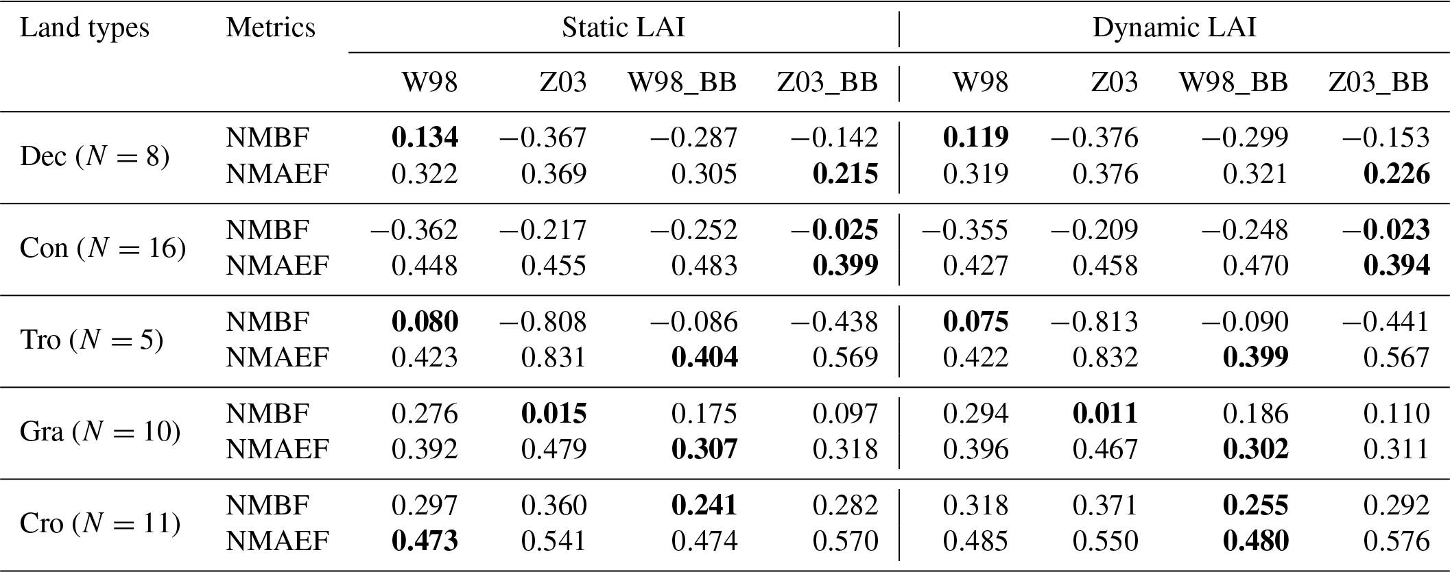
The performance metrics of each parameterization at each land type are summarized in Table 2. Comparing the two multiplicative parameterizations (W98 and Z03), we find that W98 performs satisfactorily over deciduous forests and tropical rainforests, while strongly underestimating daytime vd over coniferous forests. In contrast, Z03 performs better in coniferous forests but worse in tropical rainforests and deciduous forests. The severe underestimation of daytime vd by Z03 over tropical rainforests has previously been attributed to persistent canopy wetness and hence stomatal blocking imposed by the parameterization (Centoni, 2017). We also note that even for the same location, vd can vary significantly between seasons (Rummel et al., 2007) and management practices (Fowler et al., 2011), which models may fail to capture due to limited representations of land cover. Given the small sample size (N=5), diverse environments, and large anthropogenic intervention in the tropics, the disparity in performance metrics may not fully reflect the relative model performance. Baseline cuticular resistance in Z03 under dry and wet canopy is 1.5 and 2 times that of coniferous forests, respectively (Zhang et al., 2003), such that the enhancement of cuticular uptake by wetness may not compensate the reduced gs over tropical rainforests, and, to a lesser extent, deciduous forests.
Over grasslands, W98 has higher positive biases, while Z03 has higher absolute errors. This is because for datasets at high latitudes, the dominant grass PFT is arctic grass, which is mapped to “tundra” land type (Geddes et al., 2016). While tundra is parameterized similarly to grasslands in W98, this is not the case in Z03. Combined with the general high biases at other sites for these parameterizations, the large low biases for “tundra” sites in Z03 lower the overall high biases but lead to higher absolute errors.
Over croplands, the positive biases and absolute errors are relatively large for both W98 and Z03 (with Z03 performing worse in general than W98). The functional and physiological diversity with the “crop” land type also contributes to the general difficulty in simulating vd over cropland. Even though Z03 has individual parameterizations for four specific crop types (rice, sugar, maize, and cotton), this advantage is difficult to fully leverage, as most global land cover datasets do not resolve croplands in such detail. Having land cover maps that distinguish between more crop types could potentially improve the performance of Z03. The evaluation for herbaceous land types also suggests that as CLM PFTs do not have exact correspondence with W98 and Z03 land types, our results over herbaceous land types are subject to the uncertainty in land-type mapping (e.g. tundra vs. grassland, specific vs. generic crops, C3 vs. C4 grass).
Substituting the native gs in W98 and Z03 by that simulated by the Ball–Berry model (the W98_BB and Z03_BB runs) generally, though not universally, leads to improvement in model performance against the observations. W98_BB has considerably smaller biases and absolute errors than W98 over grassland. While having little effect on the absolute error, W98_BB improves the biases over coniferous forest and cropland compared to W98 but worsens the biases over rainforests and deciduous forests. In contrast, Z03_BB is able to improve the model–observation agreement over all five land types when compared to Z03. This finding echoes that from Wu et al. (2011), who explicitly show the advantage of replacing the gs of Wesely (1989) with the Ball–Berry model in simulating vd over a forest site and in addition show the potential of the Ball–Berry model in improving the spatial distribution of mean vd. The different responses to substituting native gs with that from the Ball–Berry model highlight the significant differences in parameterizing non-stomatal uptake between W98 and Z03, which further suggests that the uncertainty in non-stomatal deposition should not be overlooked.
The minimal impact that results from using LAI that matches the time of observation is not unexpected, since the meteorological and land cover information from a 2∘ × 2.5∘ grid cell may not be representative of the typical footprint of a site measurement (on the order of 10−3 to 101 km2, e.g. Chen et al., 2009, 2012). The mismatch between model resolution and the footprint of site-level measurements has also been highlighted in previous evaluation efforts in global-scale CTMs (Hardacre et al., 2015; Silva and Heald, 2018). Furthermore, the sample sizes for all land types are small (N≤16) and the evaluation may be further compromised by inherent sampling biases.
In addition to the evaluation against field observation, we find good correlation (R2=0.94) between the annual mean vd from GEOS-Chem at 2013 and the 30-year mean vd of W98 run with static LAI, providing further evidence that our implementation of W98 is reliable. Overall, our evaluation shows that the quality of our offline simulation of dry deposition across the four parameterizations in this work is largely consistent with previous global modelling evaluation efforts.
Here, we summarize the impact that the different dry deposition parameterizations may have on simulations of the spatial distribution of vd and on the inferred surface O3 concentrations. We begin by comparing the simulated long-term mean vd across parameterizations, then use a chemical transport model sensitivity experiment to estimate the O3 impacts.
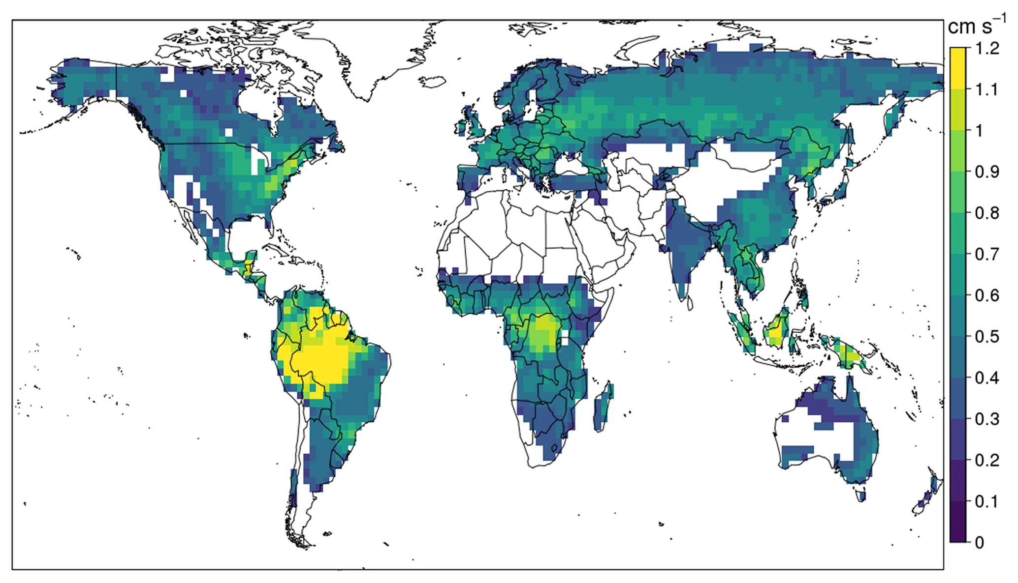
Figure 2The 1982–2011 July mean daytime vd (solar elevation angle > 20∘) over vegetated land surface simulated by W98.
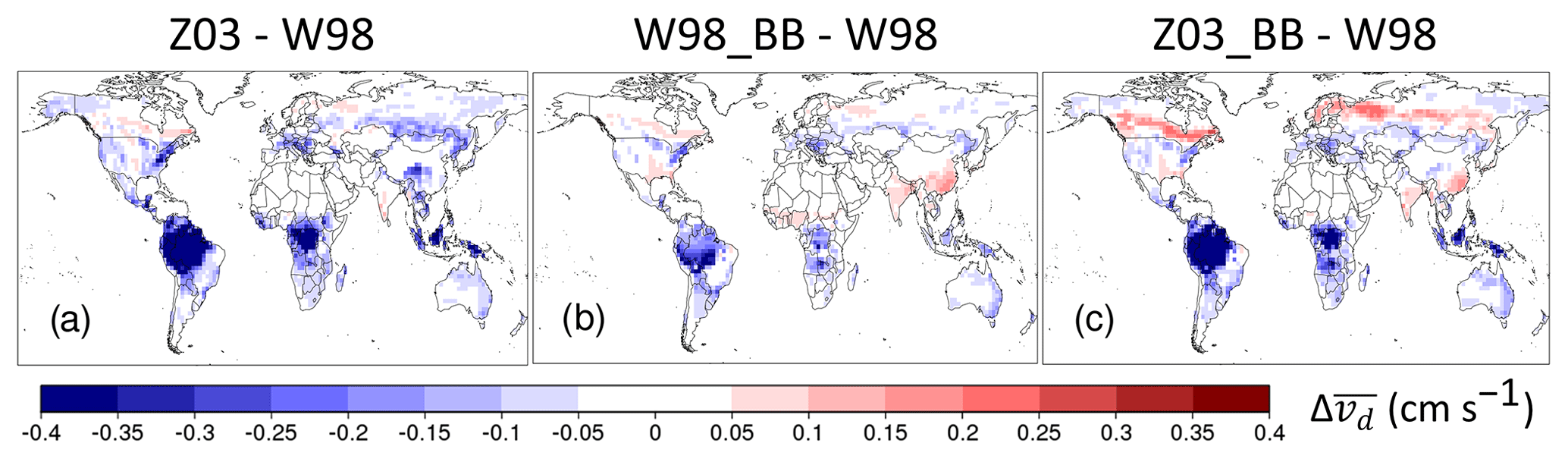
Figure 3Differences of 1982–2011 July mean daytime vd () between three other parameterizations (Z03, W98_BB, and Z03_BB) and W98 over vegetated land surface.
Figure 2 shows the 30-year July daytime average vd simulated by W98 over vegetated surfaces (defined as the grid cells with > 50 % plant cover), and Fig. 3 shows the difference between the W98 and the W98_BB, Z03, and Z03_BB predictions, respectively. We first focus on results from July because of the coincidence of high surface O3 level, biospheric activity, and vd in the Northern Hemisphere (NH) and will subsequently discuss the result for December, when such a condition holds for the Southern Hemisphere (SH). W98 simulates the highest July mean daytime vd in Amazonia (1.2 to 1.4 cm s−1), followed by other major tropical rainforests, and temperate forests in the northeastern US. July mean daytime vd in other temperate regions in North America and Eurasia typically ranges from 0.5 to 0.8 cm s−1, while in South American and the African savannah, and most parts of China, daytime vd is around 0.4 to 0.6 cm s−1. In India, Australia, the western US, polar tundra, and Mediterranean region, July mean daytime vd is low (0.2–0.5 cm s−1).
The other three parameterizations (W98_BB, Z03, Z03_BB) simulate substantially different spatial distributions of daytime vd. In North America, we find W98_BB, Z03, and Z03_BB produce lower vd (by −0.1 to −0.4 cm s−1) compared to W98 in the deciduous-forest-dominated northeastern US and slightly higher vd in boreal-forest-dominated regions of Canada. Z03 and Z03_BB produce noticeably lower vd (by up to −0.2 cm s−1) in arctic tundra and grasslands in the western US. In the southeastern US, W98_BB and Z03_BB simulate a slightly higher vd (by up to +0.1 cm s−1), while Z03 suggests a slightly lower vd (by up to −0.1 cm s−1). W98_BB simulates a lower (−0.1 to −0.4 cm s−1) vd in tropical rainforests, with larger reductions concentrated in southern Amazonia, where July is within the dry season, while the northern Amazonia is not (Malhi et al., 2008). Z03 and Z03_BB simulate much smaller (−0.4 to −0.6 cm s−1) vd in all tropical rainforests.
Over the midlatitudes in Eurasia, Australia, and South America except Amazonia, W98_BB, Z03, and Z03_BB generally simulate a lower daytime vd by up to 0.25 cm s−1, possibly due to the dominance of grasslands and deciduous forests, where W98 tends to be more high biased than other parameterizations when compared to the observations of vd. In the southern African savannah, W98_BB and Z03_BB suggest a much lower daytime vd (by −0.1 to −0.4 cm s−1) because of explicit consideration of soil moisture limitation to An and gs (demonstrated by the spatial overlap with soil moisture stress factors shown in Fig. S2). Z03_BB simulates a particularly high daytime vd over the high-latitude coniferous forests (+0.1 to +0.3 cm s−1). W98_BB and Z03_BB produce higher daytime vd (up to +0.15 cm s−1) in India and south China due to temperature acclimation (Kattge and Knorr, 2007), which allows more stomatal opening under the high temperature that would largely shut down the stomatal deposition in W98 and Z03, as long as the soil does not become too dry to support stomatal opening. This is guaranteed by the rainfall from summer monsoon in both regions. Low vd is simulated by Z03 and Z03_BB in the grasslands near the Tibetan Plateau because the grasslands are mainly mapped to the tundra land type, which typically has low vd as discussed in Sect. 3.
Our results suggest that the global distribution of simulated mean vd depends substantially on the choice of dry deposition parameterization, driven primarily by the response to hydroclimate-related parameters such as soil moisture, VPD, and leaf wetness, in addition to land-type-specific parameters, which could impact the spatial distribution of surface ozone predicted by chemical transport models. To estimate the impact on surface ozone of an individual parameterization “i” compared to the W98 predictions (which we use as a baseline), we apply the following equation:
where ΔO3,i is the estimated impact on simulated O3 concentrations in a grid box, is the difference between parameterization i and W98 simulated mean daytime vd in that grid box, is W98 output mean daytime vd for that grid box, and β is the sensitivity of surface ozone to vd calculated by the method outlined in Sect. 2.3.
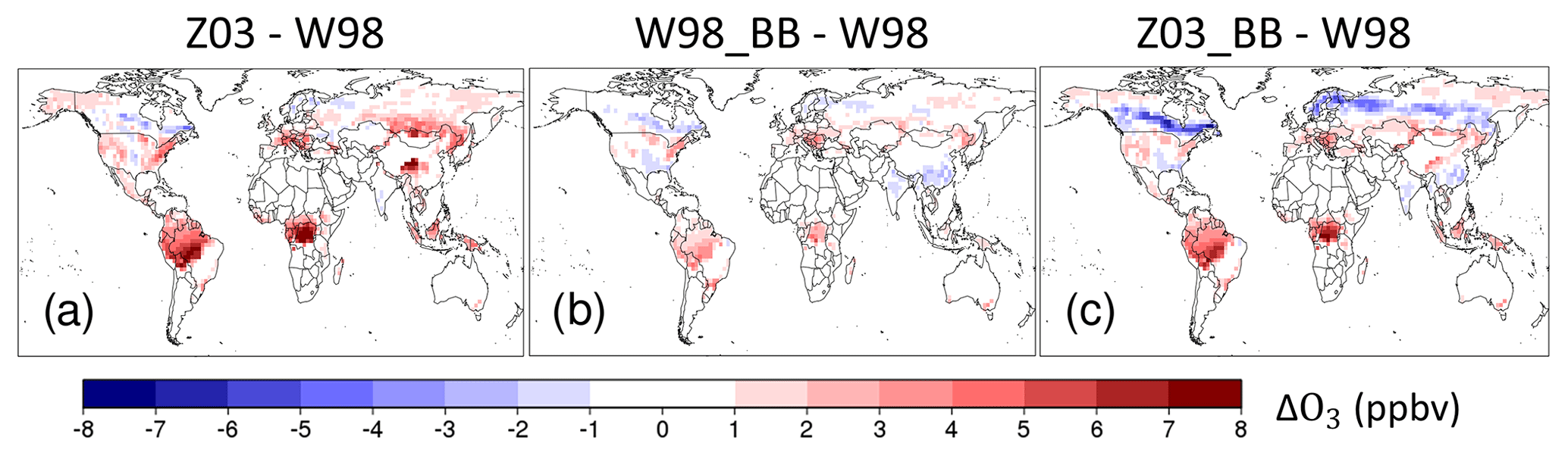
Figure 4Estimated difference in July mean surface ozone (ΔO3) due to the discrepancy of simulated July mean daytime vd among the parameterizations.
Figure 4 shows the resulting estimates of ΔO3 globally. We find ΔO3 is the largest in tropical rainforests for all the parameterizations (up to 5 to 8 ppbv). Other hotspots of substantial differences are boreal coniferous forests, the eastern US, continental Europe, Eurasian steppe, and the grassland in southwestern China, where ΔO3 is either relatively large or the signs disagree among parameterizations. In India, Indochina, and south China, ΔO3 is relatively small but still reaches up to up to −2 ppbv. We find that ΔO3 is not negligible (1–4 ppbv) in many regions with relatively high population density, which suggests that the choice of dry deposition parameterization can be relevant to the uncertainty in the study of air quality and its implication on public health. We note that we have not estimated ΔO3 for some regions with low GEOS-Chem-predicted vd (< 0.25 cm s−1, as described in Sect. 2.3) but where the disagreement in vd between parameterizations can be large (e.g. the southern African savannah; see Fig. 3). Given this limitation, the impacts on O3 we have summarized may therefore be spatially conservative.
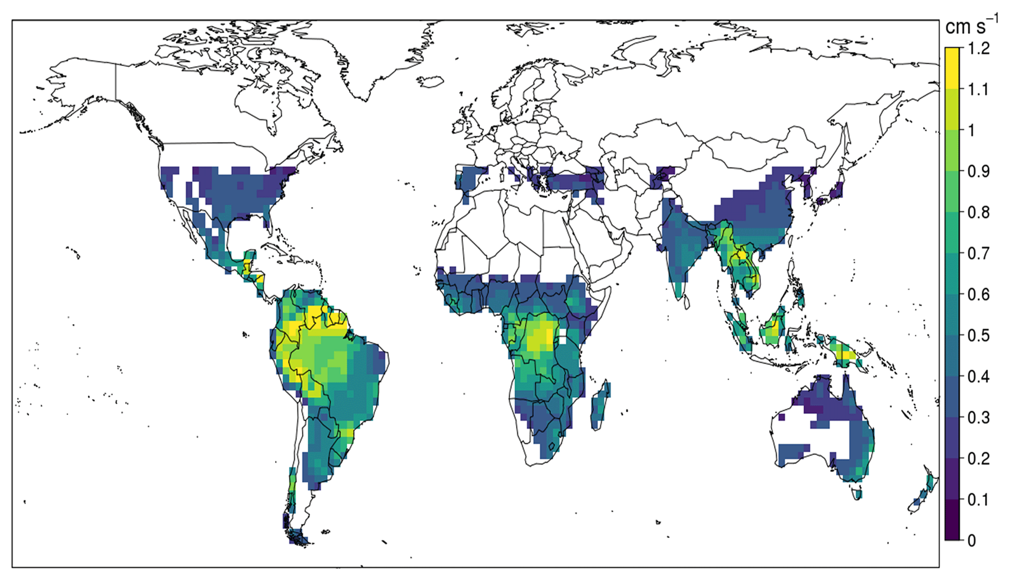
Figure 5The 1982–2011 December mean daytime vd (solar elevation angle > 20∘) over vegetated land surface simulated by W98. The data over high latitudes over Northern Hemisphere are invalid due to insufficient daytime hours over the month (< 100 h month−1).
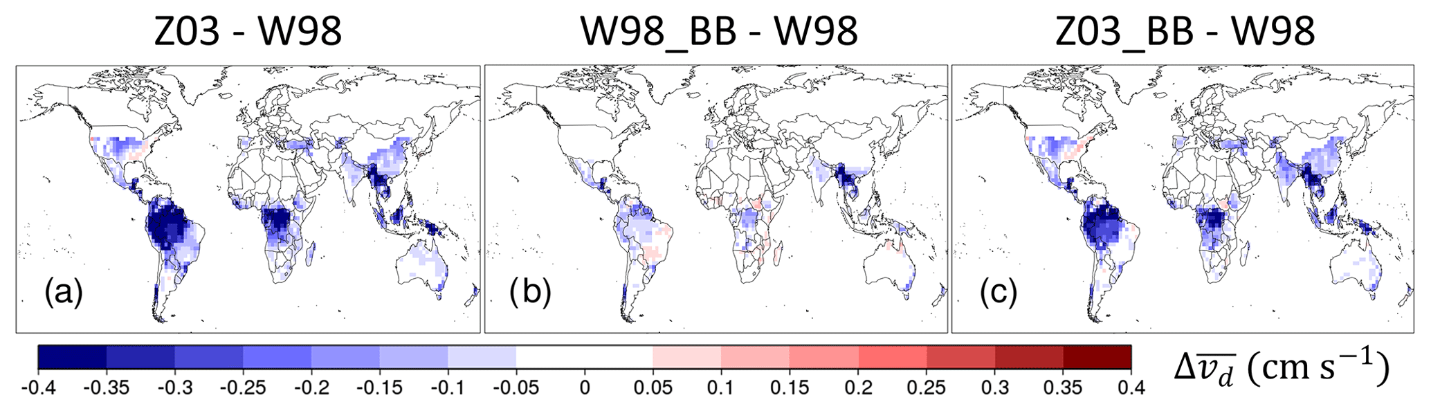
Figure 6Differences of 1982–2011 December mean daytime vd () between three other parameterizations (Z03, W98_BB, and Z03_BB) and W98 over vegetated land surface.
To explore the impact of different prediction of vd on surface O3 in different seasons, we repeat the above analyses for December. Figure 5 shows the 1982–2011 mean December daytime vd predicted by W98, while Fig. 6 shows the difference between W98 and the Z03, W98_BB, and Z03_BB, respectively. High latitudes in the NH are excluded due to the small number of daytime hours. Z03 and Z03_BB simulate substantially lower in daytime vd at NH midlatitudes because Z03 and Z03_BB allow partial snow cover but W98 and W98_BB only allow total or no snow cover. At midlatitudes, the snow cover is not high enough to trigger the threshold of converting vegetated to snow-covered ground in W98 and W98_BB, resulting in lower surface resistance, and hence higher daytime vd compared to Z03 and Z03_BB; in Amazonia, the hotspot of difference in daytime vd shifts from the south to the north relative to July, which is in the dry season (Malhi et al., 2008). These results for December, together with our findings from July, suggest that the discrepancy in simulated daytime vd between W98 and other parameterizations is due to the explicit response to hydroclimate in the former compared to the latter. Given that field observations indicate a large reduction of vd in dry season in Amazonia (Rummel et al., 2007), the lack of dependence of hydroclimate can be a drawback of W98 in simulating vd in Amazonia.
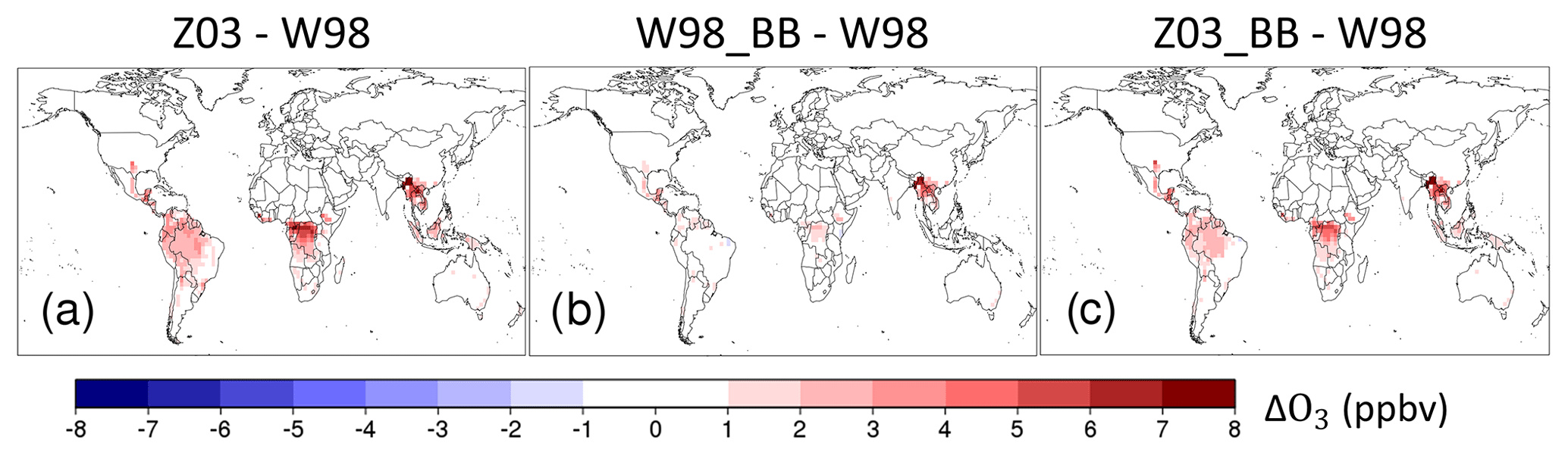
Figure 7Estimated difference in December mean surface ozone (ΔO3) due to the discrepancy of simulated December mean daytime vd among the parameterizations.
Figure 7 shows the resulting estimates of ΔO3 globally for December using Eq. (3). In all major rainforests, ΔO3 is smaller in December due to generally lower sensitivity compared to July. A surprising hotspot of both daytime Δvd and ΔO3 is the rainforest/tropical deciduous forest in Myanmar and its eastern bordering region, which also has distinct wet and dry seasons. The proximity of December to the dry season, which starts in January (e.g. Matsuda et al., 2005), indicates that the consistent Δvd between W98 and other parameterizations is driven by hydroclimate as in Amazonia. Comparison with field measurements (Matsuda et al., 2005) suggests that the W98_BB and Z03_BB capture daytime vd better than W98, while Z03 may overemphasize the effect of such dryness. The above reasoning also explains some of the Δvd in India and south China across the three parameterizations. These findings identify hydroclimate as a key driver of process uncertainty of vd over tropics and subtropics, and therefore its impact on the spatial distribution of surface ozone concentrations, independent of land-type-based biases, in these regions.
Overall, these results demonstrate that the discrepancy in the spatial distribution of simulated mean daytime vd resulting from choice of dry deposition parameterization can have an important impact on the global distribution of surface O3 predicted by chemical transport models. We find that the response to hydroclimate by individual parameterization not only affects the mean of predicted surface ozone but also has different impacts in different seasons, which is complementary to the findings of Kavassalis and Murphy (2017) that mainly focus on how shorter-term hydrometeorological variability may modulate surface O3 through dry deposition.
Here, we explore the impact that different dry deposition parameterizations may have on predictions of IAV and trends in vd and on the inferred surface O3 concentrations. We use the Theil–Sen method (Sen, 1968), which is less susceptible to outliers than least-square methods, to estimate trends in July daytime vd (and any underlying meteorological variables) and use p value < 0.05 to estimate significance.

Figure 8Trends of July mean daytime vd during 1982–2011 over vegetated land surface. Black dots indicate statistically significant trends (p<0.05).

Figure 9Estimated impact of trends of July mean daytime vd on July mean surface ozone () during 1982–2011 over vegetated land surface. Only grid points with statistically significant trends (p<0.05) in July mean daytime vd are considered.
Figure 8 shows the trend in July mean daytime vd from 1982 to 2011 predicted by each of the parameterizations and scenarios ([Clim], [Clim + LAI], and [Clim + LAI + CO2]). Figure 9 shows the potential impact of these trends in vd on July daytime surface ozone, which we estimate to a first order using the following equation:
where and are the absolute change in ozone inferred to a first order as a result of the trend of vd and the normalized Theil–Sen slope (% yr−1) of vd for parameterization i over the 30 years (1982–2011).
In [Clim] simulations (where LAI is held constant), significant decreasing trends in July daytime vd are simulated by the Z03, W98_BB, and Z03_BB in Mongolia, where significant increasing trend in T (warming) and decreasing trend in RH (drying) detected in the MERRA-2 surface meteorological field in July daytime. This trend is not present in the W98 parameterization as this formulation does not respond to the long-term drying. We find some decreasing trends in vd across parts of central Europe and the Mediterranean to varying degrees across the parameterizations. In the SH, we find consistent decreasing trends across all four parameterizations in southern Amazonia and southern African savannah due to warming and drying, which we estimate could produce a concomitant increase in July mean surface ozone of between 1 to 3 ppbv (Fig. 9).
In [Clim + LAI] scenario, all four parameterizations simulate a significant increasing trend of vd over high latitudes, which is consistent with the observed greening trend over the region (Zhu et al., 2016). We estimate this could produce a concomitant decrease in July mean surface ozone of between 1 and 3 ppbv. The parameterizations generally agree in terms of the spatial distribution of these trends in O3. Exceptions include a steeper decreasing trend in most of Siberia predicted by W98, while the trend is more confined in eastern and western Siberia in the other three parameterizations. Including the effect of CO2-induced stomatal closure ([Clim + LAI + CO2] runs) partially offsets the increase of vd in high latitudes but does not lead to large changes in both the magnitudes and spatial patterns of vd trend. We find negligible trends in daytime vd for December in all cases. These results show that across all dry deposition model parameterizations, LAI and climate, more than increasing CO2, can potentially drive significant long-term changes in vd and should not be neglected when analysing the long-term change in air quality over 1982–2011. We note that the importance of the CO2 effect could grow as the period of study extends to allow a larger range of atmospheric CO2 concentrations (Hollaway et al., 2017; Sanderson et al., 2007).
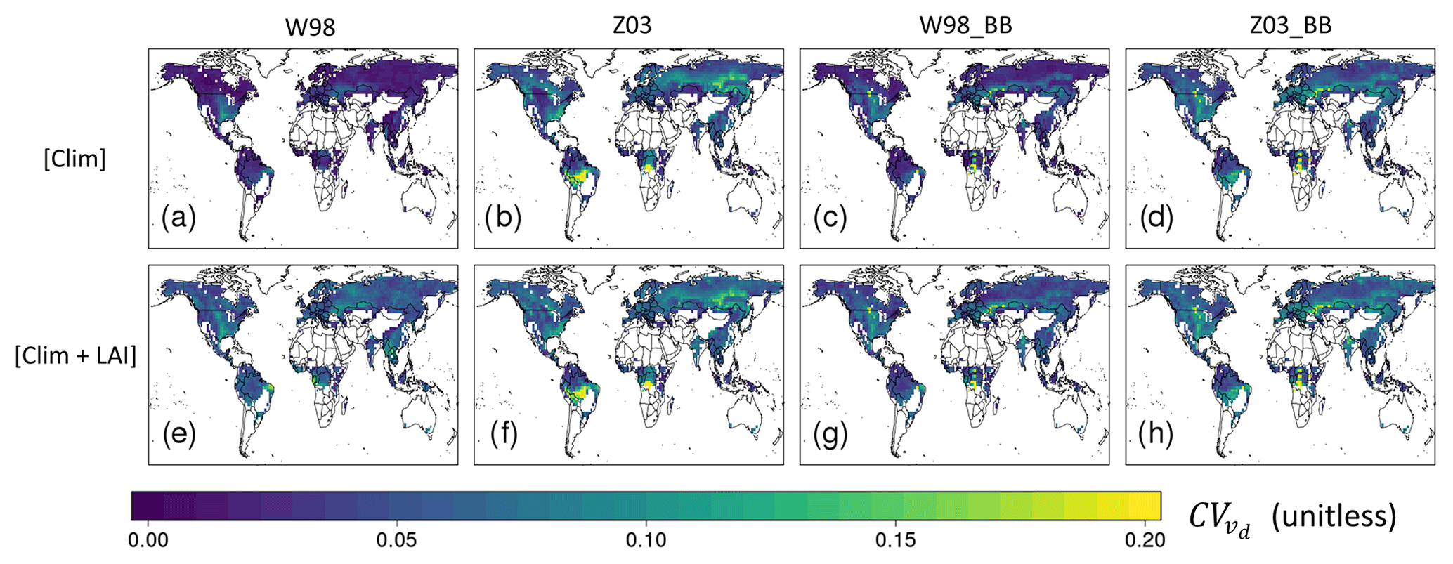
Figure 10Interannual coefficient of variation of linearly detrended July mean daytime vd (CV) during 1982–2011 over vegetated land surface.

Figure 11Estimated contribution of IAV in July mean daytime vd to IAV of July mean surface ozone () during 1982–2011 over vegetated land surface.
We go on to explore the impact of parameterization choice in calculations of IAV in vd. Figure 10 shows the coefficient of variation of linearly detrended July daytime vd (CV). Figure 11 shows the potential impact this has on IAV in surface ozone, which we estimate to a first order by the following equation:
where is the estimated interannual standard deviation in surface ozone resulting from IAV in vd given predicted by dry deposition parameterization i. In both cases, we show only the [Clim] and [Clim + LAI] runs, since IAV in CO2 has negligible impact on interannual variability in vd.
Using the W98 parameterization, IAV in predicted vd and O3 is considerably smaller in the [Clim] run than that for the [Clim + LAI] run, since both the stomatal and non-stomatal conductance in W98 are assumed to be strong functions of LAI rather than meteorological conditions. This implies that long-term simulations with W98 and constant LAI can potentially underestimate the IAV of vd and surface ozone. In contrast, IAV in vd calculated by the Z03 parameterization is nearly the same for the [Clim] and [Clim + LAI] runs. In Z03, gs is also directly influenced by VPD in addition to temperature and radiation, and non-stomatal conductance in Z03 is much more dependent on meteorology than W98, leading to high sensitivity to climate. Though the Ball–Berry model also responds to meteorological conditions, it considers relatively complex An–gs regulation and includes temperature acclimation, which could dampen its sensitivity to meteorological variability compared to the direct functional dependence on meteorology in the Z03 multiplicative algorithm. Thus, the climate sensitivity of W98_BB and Z03_BB is in between Z03 and W98, as is indicated by a more moderate difference between from [Clim] and [Clim + LAI] runs in Fig. 11.
For regional patterns of CV and , we focus on the [Clim + LAI] runs (Figs. 10e to h and 11e to h) as they allow for a comparison of all four parameterizations and contain all the important factors of controlling vd. In North America, we estimate modest IAV in vd across all four parameterizations (CV < 15 %) in most places. We find this results in relatively low in the northeastern US and larger in the central and southeast US (in the range of 0.3 to 2 ppbv). These results are of a similar magnitude to the standard deviation of summer mean background ozone suggested by Fiore et al. (2014) over similar time period, suggesting that IAV of dry deposition can be a potentially important component of the IAV of surface ozone in summer over North America.
All parameterizations produce larger CV (and therefore larger in southern Amazonia compared to northern and central Amazonia, but we find substantial discrepancies across parameterizations. The estimated impact on IAV in O3 in southern Amazonia ranges from less than 1 ppbv, predicted by the W98 and W98_BB parameterizations, to exceeding 1.5–2.5 ppbv predicted by the Z03 parameterization. IAV is also relatively large in central Africa. We find that the parameterizations which include a Ball–Berry formulation (W98_BB and Z03_BB) estimate higher IAV in this region (with varying between 1 and 4 ppbv), compared to the W98 and Z03 parameterizations ( up to 2 ppbv). We also note that the Ball–Berry formulations show more spatial heterogeneity compared to W98 and Z03. In our implementation of the Ball–Berry model, impact of soil moisture on gs is parameterized as a function of root-zone soil matric potential, which makes gs very sensitive to variation in soil wetness when its climatology is near the point that triggers limitation on An and gs. Given the large uncertainty in global soil property map (Dai et al., 2019), such sensitivity could be potentially artificial, which should be taken into consideration when implementing Ball–Berry parameterizations in large-scale models despite their relatively good performance in site-level evaluation (Wu et al., 2011).
Across Europe, the magnitudes of IAV predicted by all four parameterizations show relatively good spatial consistency. Simulated CV is relatively low in western and northern Europe (< 10 %), which we estimate translates to less than 1 ppbv of . We find larger CV (and therefore large over parts of southern Russia and Siberia ( up to 2.5 ppbv) from all parameterizations except W98. The local geographic distribution of CV and also significantly differs among the parameterizations there. Z03 and Z03_BB simulate larger CV in eastern Siberia than W98_BB, while W98 BB and Z03_BB predict larger CV over the southern Russian steppe then Z03. Finally, all four parameterizations estimate relatively low CV and in India, China, and southeast Asia.
We compare the simulated IAV July CV from all four deposition parameterizations with those recorded by publicly available long-term observations. Hourly vd is calculated using Eq. (1) from raw data. We filter out the data points with extreme (> 2 cm s−1) or negative vd, and without enough turbulence (u∗ < 0.25 m s−1). As vd values in each daytime hour are not uniformly sampled in the observational datasets, we calculate the mean diurnal cycle and then calculate the daytime average July vd for each year from the mean diurnal cycle, from which CV can be calculated.
The IAV predicted by all four parameterizations at Harvard Forest is between 3 % and 7.9 %, which is 2 to 6 times lower than that presented in the observations (18 %). We find similar underestimations by all four parameterizations compared to the long-term observation from Hyytiälä (Junninen et al., 2009; Keronen et al., 2003; https://avaa.tdata.fi/web/smart/smear/download, last access: 25 July 2019), where observed CV (16 %) is significantly higher than that predicted by the deposition parameterizations (3.5 %–7.1 %). In Blodgett Forest, we find that the models underestimate the observed annual CV more seriously (∼1 %–3 % compared to 18 % in the observations). This suggests that the IAV of vd may be underestimated across all deposition parameterizations we investigated (and routinely used in simulations of chemical transport). Clifton et al. (2019) attribute this to the IAV in deposition to wet soil and dew-wet leaves, and in-canopy chemistry under stressed conditions for forests over the northeastern US. Some of these processes (e.g. in-canopy chemistry, wetness slowing soil ozone uptake) are not represented by existing parameterizations, contributing to their difficulty in reproducing the observed IAV. The scarcity of long-term ozone flux measurements (Fares et al., 2010, 2017; Munger et al., 1996; Rannik et al., 2012) limits our ability to benchmark the IAV in our model simulations with observational datasets.
In summary, when both the variability in LAI and climate are considered, the IAV in simulated vd translates to IAV in surface O3 of 0.5–2 ppbv in July for most regions. Such variability is predicted to be particularly strong in southern Amazonian and central African rainforest, where the predicted IAV in July surface O3 due to dry deposition can be as high as 4 ppbv. This suggests that IAV of vd can be an important part of the natural variability of surface O3. The estimated magnitude of IAV is also dependent of the choice of vd parameterization, which highlights the importance of vd parameterization choice on modelling IAV of surface O3.
We present the results of multidecadal global modelling of ozone dry deposition using four different ozone deposition parameterizations that are representative of the major types of approaches of gaseous dry deposition modelling used in global chemical transport models. The parameterizations are driven by the same assimilated meteorology and satellite-derived LAI, which minimizes the uncertainty of model input across parameterization and simplifies interpretation of inter-model differences. The output is evaluated against field observations and shows satisfactory performance. One of our main goals was to investigate the impact of dry deposition parameterization choice on long-term averages, trends, and IAV in vd over a multidecadal timescale and estimate the potential concomitant impact on surface ozone concentrations to a first order using a sensitivity simulation approach driven by the GEOS-Chem chemical transport model.
We find that the performance of the four dry deposition parameterizations against field observations varies considerably over land types, and these results are consistent with other evaluations, reflecting the potential issue that dry deposition parameterizations can often be overfit to a particular set of available observations, requiring caution in their application at global scales. We also find that using more ecophysiologically realistic output gs predicted by the Ball–Berry model can generally improve model performance but at the cost of high sensitivity to relatively unreliable soil data. However, the number of available datasets of ozone dry deposition observation is still small and concentrated in North America and Europe. We know of only one multi-season direct observational record in Asia (Matsuda et al., 2005) and none in Africa, where air quality can be an important issue. To better constrain regional O3 dry deposition, effort must be made in making new observations of gaseous dry deposition (Fares et al., 2017) especially in the undersampled regions. Evaluation and development of ozone dry deposition parameterizations will continue to benefit from publicly available ozone flux measurements and related micrometeorological variables that allow for partitioning measured flux into individual deposition pathways (e.g. Clifton et al., 2017, 2019; Fares et al., 2010; Wu et al., 2011, 2018).
We find substantial disagreement in the spatial distribution between the mean daytime vd predicted by the different parameterizations we tested. We find that these discrepancies are in general a function of both location and season. In NH summer, vd values simulated by the four parameterizations are considerably different in many regions over the world. We estimate that this could lead to around 2 to 5 ppbv in uncertainty of surface ozone concentration simulations over a vast majority of land in the NH. In tropical rainforests, where leaf wetness is prevalent and the dry–wet season dynamics can have a large impact on vd (Rummel et al., 2007), we estimate the uncertainty due to dry deposition model choice could even lead to an uncertainty in surface ozone of up to 8 ppbv. We also find noticeable impacts in parameterization choice during SH summer, but we note that due to the unreliability of β at low vd, we have not assessed its impact on surface ozone in many high-latitude regions of the NH. In general, we find hydroclimate to be an important driver of the uncertainty. This demonstrates that the potential impact of parameterization choice (or process uncertainty) of vd is neither spatiotemporally uniform nor negligible in many regions over the world. More multi-seasonal observations are especially needed over seasonally dry ecosystems where the role of hydroclimate in deposition parameterizations needs to be evaluated. Recently, standard micrometeorological measurements have been used to derive gs and stomatal deposition of O3 over North America and Europe (Ducker et al., 2018), highlighting the potential of using global networks of micrometeorological observation (e.g. FLUXNET; Baldocchi et al., 2001) to benchmark and calibrate gs of dry deposition parameterizations, which could at least increase the spatiotemporal representativeness, if not the absolute accuracy, of dry deposition parameterizations, since it would be difficult to constrain non-stomatal sinks with this method. Further research is required to more directly verify whether better-constrained gs leads to improved vd simulation.
Over the majority of vegetated regions in the NH, we estimate the IAV of mean daytime vd is generally on the order of 5 % to 15 % and may contribute between 0.5 and 2 ppbv of IAV in July surface O3 over the 30-year period considered here, with each parameterization simulating different geographic distribution of where IAV is highest. The predicted IAV from all four models is smaller than what long-term observations suggest, but its potential contribution to IAV in O3 is still comparable to the long-term variability of background ozone over similar timescales in US summer (Brown-Steiner et al., 2018; Fiore et al., 2014). This would seem to confirm that vd may be a substantial contributor to natural IAV of O3 in summer, at least in the US. In the Southern Hemisphere, the IAV mainly concentrates in the drier part of tropical rainforests. The Ball–Berry parameterizations simulate large and spatially discontinuous CV and due to their sensitivity to soil wetness. Globally, we find that IAV of vd in W98 is mostly driven by LAI, while in other parameterizations climate generally plays a more important role. We therefore emphasize that temporal matching of LAI is important for consistency when W98 is used in long-term simulations. While our results show notable impacts across the globe, in many regions there are no available long-term observations to evaluate the model predictions over interannual timescales. This information is helpful in designing and identifying sources of error in model experiments that involve variability of vd.
We are also able to detect statistically significant trends in July daytime vd over several regions. The magnitudes of trends are up to 1 % per year and both climate and LAI contribute to the trend. All four deposition parameterizations identify three main hotspots of decreasing July daytime vd (southern Amazonia, southern African savannah, Mongolia), which we link mainly to increasing surface air temperature and decreasing relative humidity. Meanwhile, extensive areas at high latitudes experience LAI-driven increasing July daytime vd, consistent with the greening trend in the region (Zhu et al., 2016). We do not find a strong influence of CO2-induced stomatal closure in the trend over this time period. Over the 30 years, we estimate the trend in July daytime vd could translate approximately to 1 to 3 ppbv of ozone changes in the areas of impact, indicating the potential effect of long-term changes in vd on surface ozone. This estimate should be considered conservative, since we are unable to reliably test the sensitivity of ozone to regions with low vd with our approach.
While the approach we have presented here allows us to explore the role of dry deposition parameterization choice on simulations of long-term means, trends, and IAV in ozone dry deposition velocity, there remain some limitations and opportunities for development. First, we only used one LAI and assimilated meteorological product. The geographic distribution of trend and IAV of vd may vary considerably as the LAI and meteorological products used due to their inherent uncertainty (e.g. Jiang et al., 2017). While we expect the qualitative conclusions about how LAI and climate controls the modelled trend and IAV of vd to be robust to the choice of dataset, the magnitude and spatial variability could be affected. Second, the estimated effects on surface O3 are a first-order inference based on a linear approximation of the impact that vd has directly on O3. We have not applied our analysis to regions with low GEOS-Chem vd, where other components of parameterization (e.g. definition and treatment of snow cover, difference in ground resistance) may have major impact on vd prediction (Silva and Heald, 2018), nor accounted for the role that vd variability can have on other chemical species which would have feedbacks on O3. Moreover, the sensitivity of surface ozone to vd may be dependent on the choice of chemical transport model (here, the GEOS-Chem model has been used) and possibly the choice of simulation year for the sensitivity simulation. Finally, we have neglected the effect of land use and land cover change on global PFT composition at this stage, which can be another source of variability for vd and even long-term LAI retrieval (Fang et al., 2013). Nevertheless, the relatively high NMAEF of simulated vd and the inherent uncertainty in input data (land cover, soil property, assimilated meteorology, and LAI) are considered as the major sources of uncertainty in our predictions of vd.
The impact of dry deposition parameterization choice may also have impacts which we have not explored in this study on other trace gases with deposition velocity controlled by surface resistance, and for which stomatal resistance is an important control of surface resistance (e.g. NO2). As vd has already been recognized as a major source of uncertainty in deriving global dry deposition flux of NO2 and SO2 (Nowlan et al., 2014), systematic investigation on the variability and uncertainty of vd for other relevant chemical species does not only contribute to understanding the role of gaseous dry deposition on air quality but also to biogeochemical cycling. Particularly, gaseous dry deposition has been shown to be a major component in nitrogen deposition (Geddes and Martin, 2017; Zhang et al., 2012), highlighting the potential importance of understanding the role of vd parameterization in modelling regional and global nitrogen cycles.
Here, we have built on the recent investigations of modelled global mean (Hardacre et al., 2015; Silva and Heald, 2018) and observed long-term variability (Clifton et al., 2017) of O3vd. We are able to demonstrate the substantial impact of vd parameterization on modelling the global mean and IAV of vd, and their non-trivial potential impact on simulated seasonal mean and IAV of surface ozone. We demonstrate that the parameterizations with explicit dependence on hydroclimatic variables have higher sensitivity to climate variability than those without. Lin et al. (2019) likewise recently demonstrated the importance of accounting for water availability in O3 dry deposition modelling. Difficulties in evaluating predictions of vd for many regions of the world (e.g. most of Asia and Africa) persist due to the scarcity of measurements. This makes a strong case for additional measurement and model studies of ozone dry deposition across different timescales, which would be greatly facilitated by an open data-sharing infrastructure (e.g. Baldocchi et al., 2001; Junninen et al., 2009).
The source code and output of the dry deposition parameterizations can be obtained by contacting the corresponding author (jgeddes@bu.edu).
The supplement related to this article is available online at: https://doi.org/10.5194/acp-19-14365-2019-supplement.
AYHW and JAG developed the ideas behind this study, formulated the methods, and designed the model experiments. AYHW wrote the dry deposition code and ran the chemical transport model simulations. Data analysis was performed by AYHW, with input and feedback from JAG. APKT provided the photosynthesis model code and co-supervised the dry deposition code development. SJS compiled the dry deposition observations used for evaluation. Manuscript preparation was performed by AYHW, reviewed by JAG, and commented, edited, and approved by all authors.
The authors declare that they have no conflict of interest.
We thank the Global Modelling and Assimilation Office (GMAO) at NASA Goddard Flight Center for providing the MERRA-2 data; Ranga Myneni for providing the GIMMS LAI3g product; Petri Keronen and Ivan Mammarella for the flux measurements in Hyytiälä; Silvano Fares and Allen Goldstein for the flux measurements in Blodgett Forest; and Leiming Zhang and Zhiyong Wu for the source code of Z03. Amos P. K. Tai acknowledges support from the Vice-Chancellor Discretionary Fund (project ID 4930744) from the Chinese University of Hong Kong (CUHK) given to the Institute of Environment, Energy and Sustainability. Sam J. Silva acknowledges support provided by a National Science Foundation grant to C. L. Heald (ATM-1564495).
This work was funded by a National Science Foundation CAREER grant to project PI Jeffrey A. Geddes (AGS-1750328).
This paper was edited by Tim Butler and reviewed by two anonymous referees.
Ainsworth, E. A. and Rogers, A.: The response of photosynthesis and stomatal conductance to rising [CO2]: Mechanisms and environmental interactions, Plant, Cell Environ., 30, 258–270, https://doi.org/10.1111/j.1365-3040.2007.01641.x, 2007.
Ainsworth, E. A., Yendrek, C. R., Sitch, S., Collins, W. J., and Emberson, L. D.: The Effects of Tropospheric Ozone on Net Primary Productivity and Implications for Climate Change, Annu. Rev. Plant Biol., 63, 637–661, https://doi.org/10.1146/annurev-arplant-042110-103829, 2012.
Altimir, N., Kolari, P., Tuovinen, J.-P., Vesala, T., Bäck, J., Suni, T., Kulmala, M., and Hari, P.: Foliage surface ozone deposition: a role for surface moisture?, Biogeosciences, 3, 209–228, https://doi.org/10.5194/bg-3-209-2006, 2006.
Ashworth, K., Chung, S. H., Griffin, R. J., Chen, J., Forkel, R., Bryan, A. M., and Steiner, A. L.: FORest Canopy Atmosphere Transfer (FORCAsT) 1.0: a 1-D model of biosphere–atmosphere chemical exchange, Geosci. Model Dev., 8, 3765–3784, https://doi.org/10.5194/gmd-8-3765-2015, 2015.
Avnery, S., Mauzerall, D. L., Liu, J., and Horowitz, L. W.: Global crop yield reductions due to surface ozone exposure: 1. Year 2000 crop production losses and economic damage, Atmos. Environ., 45, 2284–2296, https://doi.org/10.1016/j.atmosenv.2010.11.045, 2011.
Baldocchi, D., Falge, E., Gu, L., Olson, R., Hollinger, D., Running, S., Anthoni, P., Bernhofer, C., Davis, K., Evans, R., Fuentes, J., Goldstein, A., Katul, G., Law, B., Lee, X., Malhi, Y., Meyers, T., Munger, W., Oechel, W., Paw, U. K. T., Pilegaard, K., Schmid, H. P., Valentini, R., Verma, S., Vesala, T., Wilson, K., and Wofsy, S.: FLUXNET: A New Tool to Study the Temporal and Spatial Variability of Ecosystem-Scale Carbon Dioxide, Water Vapor, and Energy Flux Densities, B. Am. Meteorol. Soc., 82, 2415–2434, https://doi.org/10.1175/1520-0477(2001)082<2415:FANTTS>2.3.CO;2, 2001.
Baldocchi, D. D., Hicks, B. B., and Camara, P.: A canopy stomatal resistance model for gaseous deposition to vegetated surfaces, Atmos. Environ., 21, 91–101, https://doi.org/10.1016/0004-6981(87)90274-5, 1987.
Ball, J. T., Woodrow, I. E., and Berry, J. A.: A Model Predicting Stomatal Conductance and its Contribution to the Control of Photosynthesis under Different Environmental Conditions, in: Progress in Photosynthesis Research, Springer, Dordrecht, pp. 221–224., 1987.
Brook, J. R., Zhang, L., Di-Giovanni, F., and Padro, J.: Description and evaluation of a model of deposition velocities for routine estimates of air pollutant dry deposition over North America, Part I: Model development, Atmos. Environ., 33, 5037–5051, https://doi.org/10.1016/S1352-2310(99)00250-2, 1999.
Brown-Steiner, B., Selin, N. E., Prinn, R. G., Monier, E., Tilmes, S., Emmons, L., and Garcia-Menendez, F.: Maximizing ozone signals among chemical, meteorological, and climatological variability, Atmos. Chem. Phys., 18, 8373–8388, https://doi.org/10.5194/acp-18-8373-2018, 2018.
Chen, B., Black, T. A., Coops, N. C., Hilker, T., Trofymow, J. A., and Morgenstern, K.: Assessing tower flux footprint climatology and scaling between remotely sensed and eddy covariance measurements, Bound.-Lay. Meteorol., 130, 137–167, https://doi.org/10.1007/s10546-008-9339-1, 2009.
Chen, B., Coops, N. C., Fu, D., Margolis, H. A., Amiro, B. D., Black, T. A., Arain, M. A., Barr, A. G., Bourque, C. P. A., Flanagan, L. B., Lafleur, P. M., McCaughey, J. H., and Wofsy, S. C.: Characterizing spatial representativeness of flux tower eddy-covariance measurements across the Canadian Carbon Program Network using remote sensing and footprint analysis, Remote Sens. Environ., 142, 742–755, https://doi.org/10.1016/j.rse.2012.06.007, 2012.
Centoni, F.: Global scale modelling of ozone deposition processes and interaction between surface ozone and climate change A thesis presented for the degree The University of Edinburgh, University of Edinburgh, 2017.
Clifton, O. E., Fiore, A. M., Munger, J. W., Malyshev, S., Horowitz, L. W., Shevliakova, E., Paulot, F., Murray, L. T., and Griffin, K. L.: Interannual variability in ozone removal by a temperate deciduous forest, Geophys. Res. Lett., 44, 542–552, https://doi.org/10.1002/2016GL070923, 2017.
Clifton, O. E., Fiore, A. M., Munger, J. W., and Wehr, R.: Spatiotemporal Controls on Observed Daytime Ozone Deposition Velocity Over Northeastern U.S. Forests During Summer, J. Geophys. Res. Atmos., 124, 5612–5628, doi:10.1029/2018JD029073, 2019.
Collatz, G., Ribas-Carbo, M., and Berry, J.: Coupled Photosynthesis-Stomatal Conductance Model for Leaves of C4 Plants, Aust. J. Plant Physiol., 19, 519, https://doi.org/10.1071/PP9920519, 1992.
Collatz, G. J., Ball, J. T., Grivet, C., and Berry, J. A.: Physiological and environmental regulation of stomatal conductance, photosynthesis and transpiration: a model that includes a laminar boundary layer, Agric. For. Meteorol., 54, 107–136, https://doi.org/10.1016/0168-1923(91)90002-8, 1991.
Dai, Y., Shangguan, W., Wei, N., Xin, Q., Yuan, H., Zhang, S., and Liu, S.: SOIL A review of the global soil property maps for Earth system models, Soil, 5, 137–158, https://doi.org/10.5194/soil-5-137-2019, 2019.
Ducker, J. A., Holmes, C. D., Keenan, T. F., Fares, S., Goldstein, A. H., Mammarella, I., Munger, J. W., and Schnell, J.: Synthetic ozone deposition and stomatal uptake at flux tower sites, Biogeosciences, 15, 5395–5413, https://doi.org/10.5194/bg-15-5395-2018, 2018.
Emberson, L. D., Wieser, G., and Ashmore, M. R.: Modelling of stomatal conductance and ozone flux of Norway spruce: Comparison with field data, Environ. Pollut., 109, 393–402, 2000.
Fang, H., Li, W., and Myneni, R. B.: The impact of potential land cover misclassification on modis leaf area index (LAI) estimation: A statistical perspective, Remote Sens., 5, 830–844, https://doi.org/10.3390/rs5020830, 2013.
Fares, S., McKay, M., Holzinger, R., and Goldstein, A. H.: Ozone fluxes in a Pinus ponderosa ecosystem are dominated by non-stomatal processes: Evidence from long-term continuous measurements, Agric. For. Meteorol., 150, 420–431, https://doi.org/10.1016/j.agrformet.2010.01.007, 2010.
Fares, S., Savi, F., Muller, J., Matteucci, G., and Paoletti, E.: Simultaneous measurements of above and below canopy ozone fluxes help partitioning ozone deposition between its various sinks in a Mediterranean Oak Forest, Agric. For. Meteorol., 198, 181–191, https://doi.org/10.1016/j.agrformet.2014.08.014, 2014.
Fares, S., Conte, A., and Chabbi, A.: Ozone flux in plant ecosystems: new opportunities for long-term monitoring networks to deliver ozone-risk assessments, Environ. Sci. Pollut. Res., 25, 8240–8248, https://doi.org/10.1007/s11356-017-0352-0, 2017.
Farquhar, G. D., Von Caemmerer, S., and Berry, J. A.: A Biochemical Model of Photosynthetic CO2 Assimilation in Leaves of C3 Species, Planta, 149, 78–90, https://doi.org/10.1007/BF00386231, 1980.
Fiore, A. M., Oberman, J. T., Lin, M. Y., Zhang, L., Clifton, O. E., Jacob, D. J., Naik, V., Horowitz, L. W., Pinto, J. P., and Milly, G. P.: Estimating North American background ozone in U.S. surface air with two independent global models: Variability, uncertainties, and recommendations, Atmos. Environ., 96, 284–300, https://doi.org/10.1016/j.atmosenv.2014.07.045, 2014.
Foken, T.: 50 years of the Monin-Obukhov similarity theory, Bound.-Lay. Meteorol., 119, 431–447, https://doi.org/10.1007/s10546-006-9048-6, 2006.
Fowler, D., Nemitz, E., Misztal, P., di Marco, C., Skiba, U., Ryder, J., Helfter, C., Neil Cape, J., Owen, S., Dorsey, J., Gallagher, M. W., Coyle, M., Phillips, G., Davison, B., Langford, B., MacKenzie, R., Muller, J., Siong, J., Dari-Salisburgo, C., di Carlo, P., Aruffo, E., Giammaria, F., Pyle, J. A., and Nicholas Hewitt, C.: Effects of land use on surface-atmosphere exchanges of trace gases and energy in Borneo: Comparing fluxes over oil palm plantations and a rainforest, Philos. Trans. R. Soc. B Biol. Sci., 366, 3196–3209, https://doi.org/10.1098/rstb.2011.0055, 2011.
Franks, P. J., Adams, M. A., Amthor, J. S., Barbour, M. M., Berry, J. A., Ellsworth, D. S., Farquhar, G. D., Ghannoum, O., Lloyd, J., McDowell, N., Norby, R. J., Tissue, D. T., and von Caemmerer, S.: Sensitivity of plants to changing atmospheric CO2 concentration: From the geological past to the next century, New Phytol., 197, 1077–1094, https://doi.org/10.1111/nph.12104, 2013.
Fu, Y. and Tai, A. P. K.: Impact of climate and land cover changes on tropospheric ozone air quality and public health in East Asia between 1980 and 2010, Atmos. Chem. Phys., 15, 10093–10106, https://doi.org/10.5194/acp-15-10093-2015, 2015.
Ganzeveld, L., Bouwman, L., Stehfest, E., van Vuuren, D. P., Eickhout, B., and Lelieveld, J.: Impact of future land use and land cover changes on atmospheric chemistry-climate interactions, J. Geophys. Res., 115, D23301, https://doi.org/10.1029/2010JD014041, 2010.
Geddes, J. A. and Martin, R. V.: Global deposition of total reactive nitrogen oxides from 1996 to 2014 constrained with satellite observations of NO2 columns, Atmos. Chem. Phys., 17, 10071–10091, https://doi.org/10.5194/acp-17-10071-2017, 2017.
Geddes, J. A., Heald, C. L., Silva, S. J., and Martin, R. V.: Land cover change impacts on atmospheric chemistry: simulating projected large-scale tree mortality in the United States, Atmos. Chem. Phys., 16, 2323–2340, https://doi.org/10.5194/acp-16-2323-2016, 2016.
Gelaro, R., McCarty, W., Suárez, M. J., Todling, R., Molod, A., Takacs, L., Randles, C. A., Darmenov, A., Bosilovich, M. G., Reichle, R., Wargan, K., Coy, L., Cullather, R., Draper, C., Akella, S., Buchard, V., Conaty, A., da Silva, A. M., Gu, W., Kim, G. K., Koster, R., Lucchesi, R., Merkova, D., Nielsen, J. E., Partyka, G., Pawson, S., Putman, W., Rienecker, M., Schubert, S. D., Sienkiewicz, M., and Zhao, B.: The modern-era retrospective analysis for research and applications, version 2 (MERRA-2), J. Climate, 30, 5419–5454, https://doi.org/10.1175/JCLI-D-16-0758.1, 2017.
Gerosa, G., Vitale, M., Finco, A., Manes, F., Denti, A. B., and Cieslik, S.: Ozone uptake by an evergreen Mediterranean Forest (Quercus ilex) in Italy. Part I: Micrometeorological flux measurements and flux partitioning, Atmos. Environ., 39, 3255–3266, https://doi.org/10.1016/j.atmosenv.2005.01.056, 2005.
Gerosa, G., Marzuoli, R., Monteleone, B., Chiesa, M., and Finco, A.: Vertical ozone gradients above forests. Comparison of different calculation options with direct ozone measurements above a mature forest and consequences for ozone risk assessment, Forests, 8, https://doi.org/10.3390/f8090337, 2017.
Hardacre, C., Wild, O., and Emberson, L.: An evaluation of ozone dry deposition in global scale chemistry climate models, Atmos. Chem. Phys., 15, 6419–6436, https://doi.org/10.5194/acp-15-6419-2015, 2015.
Heald, C. L. and Geddes, J. A.: The impact of historical land use change from 1850 to 2000 on secondary particulate matter and ozone, Atmos. Chem. Phys., 16, 14997–15010, https://doi.org/10.5194/acp-16-14997-2016, 2016.
Hollaway, M. J., Arnold, S. R., Collins, W. J., Folberth, G., and Rap, A.: Sensitivity of midnineteenth century tropospheric ozone to atmospheric chemistry-vegetation interactions, J. Geophys. Res.-Atmos., 122, 2452–2473, https://doi.org/10.1002/2016JD025462, 2017.
Hoshika, Y., Carriero, G., Feng, Z., Zhang, Y., and Paoletti, E.: Determinants of stomatal sluggishness in ozone-exposed deciduous tree species, Sci. Total Environ., 481, 453–458, https://doi.org/10.1016/j.scitotenv.2014.02.080, 2014.
Hu, L., Jacob, D. J., Liu, X., Zhang, Y., Zhang, L., Kim, P. S., Sulprizio, M. P., and Yantosca, R. M.: Global budget of tropospheric ozone: Evaluating recent model advances with satellite (OMI), aircraft (IAGOS), and ozonesonde observations, Atmos. Environ., 167, 323–334, https://doi.org/10.1016/j.atmosenv.2017.08.036, 2017.
Huang, L., McDonald-Buller, E. C., McGaughey, G., Kimura, Y., and Allen, D. T.: The impact of drought on ozone dry deposition over eastern Texas, Atmos. Environ., 127, 176–186, https://doi.org/10.1016/j.atmosenv.2015.12.022, 2016.
Jacob, D. J. and Wofsy, S. C.: Budgets of Reactive Nitrogen, Hydrocarbons, and Ozone Over the Amazon Forest during the Wet Season, J. Geophys. Res., 95, 16737–16754, https://doi.org/10.1029/JD095iD10p16737, 1990.
Jacob, D. J., Fan, S.-M., Wofsy, S. C., Spiro, P. A., Bakwin, P. S., Ritter, J. A., Browell, E. V., Gregory, G. L., Fitzjarrald, D. R., and Moore, K. E.: Deposition of ozone to tundra, J. Geophys. Res., 97, https://doi.org/10.1029/91JD02696, 1992.
Jarvis, P. G.: The Interpretation of the Variations in Leaf Water Potential and Stomatal Conductance Found in Canopies in the Field, Philos. Trans. R. Soc. B Biol. Sci., 273, 593–610, https://doi.org/10.1098/rstb.1976.0035, 1976.
Jerrett, M., Burnett, R. T., Pope, C. A., Ito, K., Thurston, G., Krewski, D., Shi, Y., Calle, E., and Thun, M.: Long-Term Ozone Exposure and Mortality, N. Engl. J. Med., 360, 1085–1095, https://doi.org/10.1056/NEJMoa0803894, 2009.
Jiang, C., Ryu, Y., Fang, H., Myneni, R., Claverie, M. and Zhu, Z.: Inconsistencies of interannual variability and trends in long-term satellite leaf area index products, Glob. Chang. Biol., 23, 4133–4146, https://doi.org/10.1111/gcb.13787, 2017.
Junninen, H., Lauri, A., Keronen, P., Aalto, P., Hiltunen, V., Hari, P., and Kulmala, M.: Smart-SMEAR: On-line data exploration and visualization tool for SMEAR stations, Boreal Environ. Res., 14, 447–457, 2009.
Kattge, J. and Knorr, W.: Temperature acclimation in a biochemical model of photosynthesis: A reanalysis of data from 36 species, Plant, Cell Environ., 30, 1176–1190, https://doi.org/10.1111/j.1365-3040.2007.01690.x, 2007.
Kavassalis, S. C. and Murphy, J. G.: Understanding ozone-meteorology correlations: A role for dry deposition, Geophys. Res. Lett., 44, 2922–2931, https://doi.org/10.1002/2016GL071791, 2017.
Keeling, C. D., Stephen, C., Piper, S. C., Bacastow, R. B., Wahlen, M., Whorf, T. P., Heimann, M., and Meijer, H. A.: Exchanges of atmospheric CO2 and 13CO2 with the terrestrial biosphere and oceans from 1978 to 2000, Glob. Asp. SIO Ref. Ser. Scripps Inst. Ocean. San Diego, https://doi.org/10.1007/b138533, 2001.
Keronen, P., Reissell, a, Rannik, Ü., Pohja, T., Siivola, E., Hiltunen, V., Hari, P., Kulmala, M., and Vesala, T.: Ozone flux measurements over a Scots pine forest using eddy covariance method: Performance evaluation and comparison with flux-profile method, Boreal Environ. Res., 8, 425–443, 2003.
Kharol, S. K., Shephard, M. W., Mclinden, C. A., Zhang, L., Sioris, C. E., O'Brien, J. M., Vet, R., Cady-Pereira, K. E., Hare, E., Siemons, J., and Krotkov, N. A.: Dry Deposition of Reactive Nitrogen From Satellite Observations of Ammonia and Nitrogen Dioxide Over North America, Geophys. Res. Lett., 45, 1157–1166, https://doi.org/10.1002/2017GL075832, 2018.
Lamaud, E., Carrara, A., Brunet, Y., Lopez, A., and Druilhet, A.: Ozone fluxes above and within a pine forest canopy in dry and wet conditions, Atmos. Environ., 36, 77–88, https://doi.org/10.1016/S1352-2310(01)00468-X, 2002.
Lawrence, P. J. and Chase, T. N.: Representing a new MODIS consistent land surface in the Community Land Model (CLM 3.0), J. Geophys. Res.-Biogeo., 112, G01023, https://doi.org/10.1029/2006JG000168, 2007.
Li, D., Bou-Zeid, E., Barlage, M., Chen, F., and Smith, J. A.: Development and evaluation of a mosaic approach in the WRF-Noah framework, J. Geophys. Res.-Atmos., 118, 11918–11935, https://doi.org/10.1002/2013JD020657, 2013.
Lin, Y., Medlyn, B., and Duursma, R.: Optimal stomatal behaviour around the world, Nat. Clim., 5, 459–464, https://doi.org/10.1038/NCLIMATE2550, 2015.
Lin, M., Malyshev, S., Shevliakova, E., Paulot, F., Horowitz, L. W., Fares, S., Mikkelsen, T. N., and Zhang, L.: Sensitivity of ozone dry deposition to ecosystem-atmosphere interactions: A critical appraisal of observations and simulations, Global Biogeochem. Cy., 3, https://doi.org/10.1029/2018GB006157, 2019.
Lombardozzi, D., Sparks, J. P., Bonan, G., and Levis, S.: Ozone exposure causes a decoupling of conductance and photosynthesis: Implications for the Ball-Berry stomatal conductance model, Oecologia, 169, 651–659, https://doi.org/10.1007/s00442-011-2242-3, 2012.
Lombardozzi, D., Levis, S., Bonan, G., Hess, P. G., and Sparks, J. P.: The influence of chronic ozone exposure on global carbon and water cycles, J. Climate, 28, 292–305, https://doi.org/10.1175/JCLI-D-14-00223.1, 2015.
Malhi, Y., Roberts, J. T., Betts, R. A., Killeen, T. J., Li, W., and Nobre, C. A.: Climate change, deforestation, and the fate of the Amazon, Science, 319, 169–172, https://doi.org/10.1126/science.1146961, 2008.
Mao, J., Paulot, F., Jacob, D. J., Cohen, R. C., Crounse, J. D., Wennberg, P. O., Keller, C. A., Hudman, R. C., Barkley, M. P., and Horowitz, L. W.: Ozone and organic nitrates over the eastern United States: Sensitivity to isoprene chemistry, J. Geophys. Res.-Atmos., 118, 11256–11268, https://doi.org/10.1002/jgrd.50817, 2013.
Matsuda, K., Watanabe, I., Wingpud, V., Theramongkol, P., Khummongkol, P., Wangwongwatana, S., and Totsuka, T.: Ozone dry deposition above a tropical forest in the dry season in northern Thailand, Atmos. Environ., 39, 2571–2577, https://doi.org/10.1016/j.atmosenv.2005.01.011, 2005.
McGrath, J. M., Betzelberger, A. M., Wang, S., Shook, E., Zhu, X.-G., Long, S. P., and Ainsworth, E. A.: An analysis of ozone damage to historical maize and soybean yields in the United States, P. Natl. Acad. Sci. USA, 112, 14390–14395, https://doi.org/10.1073/pnas.1509777112, 2015.
Meyers, T. P., Finkelstein, P., Clarke, J., Ellestad, T. G., and Sims, P. F.: A multilayer model for inferring dry deposition using standard meteorological measurements, J. Geophys. Res., 103, 22645, https://doi.org/10.1029/98JD01564, 1998.
Muller, J. B. A., Percival, C. J., Gallagher, M. W., Fowler, D., Coyle, M., and Nemitz, E.: Sources of uncertainty in eddy covariance ozone flux measurements made by dry chemiluminescence fast response analysers, Atmos. Meas. Tech., 3, 163–176, https://doi.org/10.5194/amt-3-163-2010, 2010.
Munger, J. W., Wofsy, S. C., Bakwin, P. S., Fan, S.-M., Goulden, M. L., Daube, B. C., Goldstein, A. H., Moore, K. E., and Fitzjarrald, D. R.: Atmospheric deposition of reactive nitrogen oxides and ozone in a temperate deciduous forest and a subarctic woodland 1. Measurements and mechanisms, J. Geophys. Res., 101657, 639–712, https://doi.org/10.1029/96JD00230, 1996.
Myneni, R. B., Hoffman, S., Knyazikhin, Y., Privette, J. L., Glassy, J., Tian, Y., Wang, Y., Song, X., Zhang, Y., Smith, G. R., Lotsch, A., Friedl, M., Morisette, J. T., Votava, P., Nemani, R. R., and Running, S. W.: Global products of vegetation leaf area and fraction absorbed PAR from year one of MODIS data, Remote Sens. Environ., 83, 214–231, https://doi.org/10.1016/S0034-4257(02)00074-3, 2002.
Norby, R. J. and Zak, D. R.: Ecological Lessons from Free-Air CO2 Enrichment (FACE) Experiments, Annu. Rev. Ecol. Evol. Syst., 42, 181–203, https://doi.org/10.1146/annurev-ecolsys-102209-144647, 2011.
Nowlan, C. R., Martin, R. V., Philip, S., Lamsal, L. N., Krotkov, N. A., Marais, E. A., Wang, S., and Zhang, Q.: Global dry deposition of nitrogen dioxide and sulfur dioxide inferred from space-based measurements, Global Biogeochem. Cy., 28, 1025–1043, https://doi.org/10.1002/2014GB004805, 2014.
Oleson, K. W., Lawrence, D. M., Bonan, G. B., Drewniak, B., Huang, M., Koven, C. D., Levis, S., Li, F., Riley, W. J., Subin, Z. M., Swenson, S. C., Thornton, P. E., Bozbiyik, A., Fisher, R., Heald, C. L., Kluzek, E., Lamarque, J.-F., Lawrence, P. J., Leung, L. R., Lipscomb, W., Muszala, S., Ricciuto, D. M., Sacks, W., Sun, Y., Tang, J., and Yang, Z.-L.: Technical Description of version 4.5 of the Community Land Model (CLM), NCAR/TN-478+STR NCAR Tech. Note, (April), NCAR/TN-503+STR, https://doi.org/10.5065/D6RR1W7M, 2013.
Olson, D. M., Dinerstein, E., Wikramanayake, E. D., Burgess, N. D., Powell, G. V. N., Underwood, E. C., D'amico, J. A., Itoua, I., Strand, H. E., Morrison, J. C., Loucks, C. J., Allnutt, T. F., Ricketts, T. H., Kura, Y., Lamoreux, J. F., Wettengel, W. W., Hedao, P., and Kassem, K. R.: Terrestrial Ecoregions of the World: A New Map of Life on Earth, Bioscience, 51, 933–938, https://doi.org/10.1641/0006-3568(2001)051[0933:TEOTWA]2.0.CO;2, 2001.
Paulson, C. A.: The Mathematical Representation of Wind Speed and Temperature Profiles in the Unstable Atmospheric Surface Layer, J. Appl. Meteorol., 9, 857–861, https://doi.org/10.1175/1520-0450(1970)009<0857:tmrows>2.0.co;2, 1970.
Pleim, J. and Ran, L.: Surface flux modeling for air quality applications, Atmosphere (Basel), 2, 271–302, https://doi.org/10.3390/atmos2030271, 2011.
Potier, E., Ogée, J., Jouanguy, J., Lamaud, E., Stella, P., Personne, E., Durand, B., Mascher, N., and Loubet, B.: Multilayer modelling of ozone fluxes on winter wheat reveals large deposition on wet senescing leaves, Agric. For. Meteorol., 211–212, 58–71, https://doi.org/10.1016/j.agrformet.2015.05.006, 2015.
Potier, E., Loubet, B., Durand, B., Flura, D., Bourdat-Deschamps, M., Ciuraru, R., and Ogée, J.: Chemical reaction rates of ozone in water infusions of wheat, beech, oak and pine leaves of different ages, Atmos. Environ., 151, 176–187, https://doi.org/10.1016/j.atmosenv.2016.11.069, 2017.
R core team: R: A language and environment for statistical computing, R Found. Stat. Comput. Vienna, Austria, available at: http://www.R-project.org/ (last access: 25 July 2019), 2017.
Ran, L., Pleim, J., Song, C., Band, L., Walker, J. T., and Binkowski, F. S.: A photosynthesis-based two-leaf canopy stomatal conductance model for meteorology and air quality modeling with WRF/CMAQ PX LSM, J. Geophys. Res., 122, 1930–1952, https://doi.org/10.1002/2016JD025583, 2017a.
Ran, L., Pleim, J., Song, C., Band, L., Walker, J. T., and Binkowski, F. S.: A photosynthesis-based two-leaf canopy stomatal conductance model for meteorology and air quality modeling with WRF/CMAQ PX LSM, J. Geophys. Res., 122, 1930–1952, https://doi.org/10.1002/2016JD025583, 2017b.
Rannik, Ü., Altimir, N., Mammarella, I., Bäck, J., Rinne, J., Ruuskanen, T. M., Hari, P., Vesala, T., and Kulmala, M.: Ozone deposition into a boreal forest over a decade of observations: evaluating deposition partitioning and driving variables, Atmos. Chem. Phys., 12, 12165–12182, https://doi.org/10.5194/acp-12-12165-2012, 2012.
Reich, P. B.: Quantifying plant response to ozone: a unifying theory, Tree Physiol., 3, 63–91, https://doi.org/10.1093/treephys/3.1.63, 1987.
Rienecker, M. M., Suarez, M. J., Todling, R., Bacmeister, J., Takacs, L., Liu, H.-C., Gu, W., Sienkiewicz, M., Koster, R. D., Gelaro, R., Stajner, I. and Nielsen, E.: The GEOS-5 Data Assimilation System – Documentation of versions 5.0.1 and 5.1.0, and 5.2.0, NASA Tech. Rep. Ser. Glob. Model. Data Assim. NASA/TM-2008-104606, https://doi.org/10.2759/32049, 2008.
Rigden, A. J. and Salvucci, G. D.: Stomatal response to humidity and CO2 implicated in recent decline in US evaporation, Glob. Chang. Biol., 23, 1140–1151, https://doi.org/10.1111/gcb.13439, 2017.
Rummel, U., Ammann, C., Kirkman, G. A., Moura, M. A. L., Foken, T., Andreae, M. O., and Meixner, F. X.: Seasonal variation of ozone deposition to a tropical rain forest in southwest Amazonia, Atmos. Chem. Phys., 7, 5415–5435, https://doi.org/10.5194/acp-7-5415-2007, 2007.
Sadiq, M., Tai, A. P. K., Lombardozzi, D., and Val Martin, M.: Effects of ozone–vegetation coupling on surface ozone air quality via biogeochemical and meteorological feedbacks, Atmos. Chem. Phys., 17, 3055–3066, https://doi.org/10.5194/acp-17-3055-2017, 2017.
Sanderson, M. G., Collins, W. J., Hemming, D. L., and Betts, R. A.: Stomatal conductance changes due to increasing carbon dioxide levels: Projected impact on surface ozone levels, Tellus B, 59, 404–411, https://doi.org/10.1111/j.1600-0889.2007.00277.x, 2007.
Sen, P. K.: Estimates of the Regression Coefficient Based on Kendall's Tau, J. Am. Stat. Assoc., 63, 1379–1389, https://doi.org/10.1080/01621459.1968.10480934, 1968.
Silva, S. J. and Heald, C. L.: Investigating Dry Deposition of Ozone to Vegetation, J. Geophys. Res.-Atmos., 123, 559–573, https://doi.org/10.1002/2017JD027278, 2018.
Simpson, D., Benedictow, A., Berge, H., Bergström, R., Emberson, L. D., Fagerli, H., Flechard, C. R., Hayman, G. D., Gauss, M., Jonson, J. E., Jenkin, M. E., Nyíri, A., Richter, C., Semeena, V. S., Tsyro, S., Tuovinen, J.-P., Valdebenito, Á., and Wind, P.: The EMEP MSC-W chemical transport model – technical description, Atmos. Chem. Phys., 12, 7825–7865, https://doi.org/10.5194/acp-12-7825-2012, 2012.
Sitch, S., Cox, P. M., Collins, W. J., and Huntingford, C.: Indirect radiative forcing of climate change through ozone effects on the land-carbon sink, Nature, 448, 791–794, https://doi.org/10.1038/nature06059, 2007.
Sun, S., Moravek, A., Trebs, I., Kesselmeier, J., and Sörgel, M.: Investigation of the influence of liquid surface films on O3 and PAN deposition to plant leaves coated with organic/inorganic solution, J. Geophys. Res.-Atmos., 121, 14239–14256, https://doi.org/10.1002/2016JD025519, 2016.
Sun, Y., Gu, L., and Dickinson, R. E.: A numerical issue in calculating the coupled carbon and water fluxes in a climate model, J. Geophys. Res.-Atmos., 117, https://doi.org/10.1029/2012JD018059, 2012.
Tai, A. P. K., Martin, M. V., and Heald, C. L.: Threat to future global food security from climate change and ozone air pollution, Nat. Clim. Change, 4, 817–821, https://doi.org/10.1038/nclimate2317, 2014.
Travis, K. R., Jacob, D. J., Fisher, J. A., Kim, P. S., Marais, E. A., Zhu, L., Yu, K., Miller, C. C., Yantosca, R. M., Sulprizio, M. P., Thompson, A. M., Wennberg, P. O., Crounse, J. D., St. Clair, J. M., Cohen, R. C., Laughner, J. L., Dibb, J. E., Hall, S. R., Ullmann, K., Wolfe, G. M., Pollack, I. B., Peischl, J., Neuman, J. A., and Zhou, X.: Why do models overestimate surface ozone in the Southeast United States?, Atmos. Chem. Phys., 16, 13561–13577, https://doi.org/10.5194/acp-16-13561-2016, 2016.
Val Martin, M., Heald, C. L. and Arnold, S. R.: Coupling dry deposition to vegetation phenology in the Community Earth System Model: Implications for the simulation of surface O3, Geophys. Res. Lett., 41, 2988–2996, https://doi.org/10.1002/2014GL059651, 2014.
Wang, Y., Jacob, D. J. and Logan, J. A.: Global simulation of tropospheric O3-NOx-hydrocarbon chemistry: 1. Model formulation, J. Geophys. Res.-Atmos., 103, 10713–10725, https://doi.org/10.1029/98JD00158, 1998.
Wesely, M. L.: Parameterization of surface resistances to gaseous dry deposition in regional-scale numerical models, Atmos. Environ., 41, 52–63, https://doi.org/10.1016/j.atmosenv.2007.10.058, 1989.
Wesely, M. L. and Hicks, B. B.: Some Factors that Affect the Deposition Rates of Sulfur Dioxide and Similar Gases on Vegetation, J. Air Pollut. Control Assoc., 27, 1110–1116, https://doi.org/10.1080/00022470.1977.10470534, 1977.
Wesely, M. L. and Hicks, B. B.: A review of the current status of knowledge on dry deposition, Atmos. Environ., 34, 2261–2282, https://doi.org/10.1016/S1352-2310(99)00467-7, 2000.
Wild, O.: Modelling the global tropospheric ozone budget: exploring the variability in current models, Atmos. Chem. Phys., 7, 2643–2660, https://doi.org/10.5194/acp-7-2643-2007, 2007.
Wittig, V. E., Ainsworth, E. A., and Long, S. P.: To what extent do current and projected increases in surface ozone affect photosynthesis and stomatal conductance of trees? A meta-analytic review of the last 3 decades of experiments, Plant Cell Environ., 30, 1150–1162, https://doi.org/10.1111/j.1365-3040.2007.01717.x, 2007.
Wolfe, G. M., Thornton, J. A., McKay, M., and Goldstein, A. H.: Forest-atmosphere exchange of ozone: sensitivity to very reactive biogenic VOC emissions and implications for in-canopy photochemistry, Atmos. Chem. Phys., 11, 7875–7891, https://doi.org/10.5194/acp-11-7875-2011, 2011.
Wong, A. Y. H., Tai, A. P. K., and Ip, Y.-Y.: Attribution and Statistical Parameterization of the Sensitivity of Surface Ozone to Changes in Leaf Area Index Based On a Chemical Transport Model, J. Geophys. Res.-Atmos., 123, 1883–1898, https://doi.org/10.1002/2017JD027311, 2018.
Wu, S., Mickley, L. J., Kaplan, J. O., and Jacob, D. J.: Impacts of changes in land use and land cover on atmospheric chemistry and air quality over the 21st century, Atmos. Chem. Phys., 12, 1597–1609, https://doi.org/10.5194/acp-12-1597-2012, 2012.
Wu, Z., Wang, X., Chen, F., Turnipseed, A. A., Guenther, A. B., Niyogi, D., Charusombat, U., Xia, B., William Munger, J., and Alapaty, K.: Evaluating the calculated dry deposition velocities of reactive nitrogen oxides and ozone from two community models over a temperate deciduous forest, Atmos. Environ., 45, 2663–2674, https://doi.org/10.1016/j.atmosenv.2011.02.063, 2011.
Wu, Z., Staebler, R., Vet, R., and Zhang, L.: Dry deposition of O3 and SO2 estimated from gradient measurements above a temperate mixed forest, Environ. Pollut., 210, 202–210, https://doi.org/10.1016/j.envpol.2015.11.052, 2016.
Wu, Z., Schwede, D. B., Vet, R., Walker, J. T., Shaw, M., Staebler, R., and Zhang, L.: Evaluation and intercomparison of five North American dry deposition algorithms at a mixed forest site, J. Adv. Model. Earth Syst., 10, 1571–1586, https://doi.org/10.1029/2017MS001231, 2018.
Wu, Z. Y., Zhang, L., Wang, X. M., and Munger, J. W.: A modified micrometeorological gradient method for estimating O3 dry depositions over a forest canopy, Atmos. Chem. Phys., 15, 7487–7496, https://doi.org/10.5194/acp-15-7487-2015, 2015.
Young, P. J., Archibald, A. T., Bowman, K. W., Lamarque, J.-F., Naik, V., Stevenson, D. S., Tilmes, S., Voulgarakis, A., Wild, O., Bergmann, D., Cameron-Smith, P., Cionni, I., Collins, W. J., Dalsøren, S. B., Doherty, R. M., Eyring, V., Faluvegi, G., Horowitz, L. W., Josse, B., Lee, Y. H., MacKenzie, I. A., Nagashima, T., Plummer, D. A., Righi, M., Rumbold, S. T., Skeie, R. B., Shindell, D. T., Strode, S. A., Sudo, K., Szopa, S., and Zeng, G.: Pre-industrial to end 21st century projections of tropospheric ozone from the Atmospheric Chemistry and Climate Model Intercomparison Project (ACCMIP), Atmos. Chem. Phys., 13, 2063–2090, https://doi.org/10.5194/acp-13-2063-2013, 2013.
Yu, S., Eder, B., Dennis, R., Chu, S.-H., and Schwartz, S. E.: New unbiased symmetric metrics for evaluation of air quality models, Atmos. Sci. Lett., 7, 26–34, https://doi.org/10.1002/asl.125, 2006.
Zhang, L., Moran, M. D. and Brook, J. R.: A comparison of models to estimate in-canopy photosynthetically active radiation and their influence on canopy stomatal resistance, Atmos. Environ., 35, 4463–4470, https://doi.org/10.1016/S1352-2310(01)00225-4, 2001.
Zhang, L., Brook, J. R., and Vet, R.: On ozone dry deposition - With emphasis on non-stomatal uptake and wet canopies, Atmos. Environ., 36, 4787–4799, https://doi.org/10.1016/S1352-2310(02)00567-8, 2002.
Zhang, L., Brook, J. R., and Vet, R.: A revised parameterization for gaseous dry deposition in air-quality models, Atmos. Chem. Phys., 3, 2067–2082, https://doi.org/10.5194/acp-3-2067-2003, 2003.
Zhang, L., Vet, R., O'Brien, J. M., Mihele, C., Liang, Z., and Wiebe, A.: Dry deposition of individual nitrogen species at eight Canadian rural sites, J. Geophys. Res.-Atmos., 114, https://doi.org/10.1029/2008JD010640, 2009.
Zhang, L., Jacob, D. J., Liu, X., Logan, J. A., Chance, K., Eldering, A., and Bojkov, B. R.: Intercomparison methods for satellite measurements of atmospheric composition: application to tropospheric ozone from TES and OMI, Atmos. Chem. Phys., 10, 4725–4739, https://doi.org/10.5194/acp-10-4725-2010, 2010.
Zhang, L., Jacob, D. J., Knipping, E. M., Kumar, N., Munger, J. W., Carouge, C. C., van Donkelaar, A., Wang, Y. X., and Chen, D.: Nitrogen deposition to the United States: distribution, sources, and processes, Atmos. Chem. Phys., 12, 4539–4554, https://doi.org/10.5194/acp-12-4539-2012, 2012.
Zhou, P., Ganzeveld, L., Rannik, Ü., Zhou, L., Gierens, R., Taipale, D., Mammarella, I., and Boy, M.: Simulating ozone dry deposition at a boreal forest with a multi-layer canopy deposition model, Atmos. Chem. Phys., 17, 1361–1379, https://doi.org/10.5194/acp-17-1361-2017, 2017.
Zhou, S. S., Tai, A. P. K., Sun, S., Sadiq, M., Heald, C. L., and Geddes, J. A.: Coupling between surface ozone and leaf area index in a chemical transport model: strength of feedback and implications for ozone air quality and vegetation health, Atmos. Chem. Phys., 18, 14133–14148, https://doi.org/10.5194/acp-18-14133-2018, 2018.
Zhu, Z., Bi, J., Pan, Y., Ganguly, S., Anav, A., Xu, L., Samanta, A., Piao, S., Nemani, R. R. and Myneni, R. B.: Global data sets of vegetation leaf area index (LAI)3g and fraction of photosynthetically active radiation (FPAR)3g derived from global inventory modeling and mapping studies (GIMMS) normalized difference vegetation index (NDVI3G) for the period 1981 to 2, Remote Sens., 5, 927–948, https://doi.org/10.3390/rs5020927, 2013.
Zhu, Z., Piao, S., Myneni, R. B., Huang, M., Zeng, Z., Canadell, J. G., Ciais, P., Sitch, S., Friedlingstein, P., Arneth, A., Cao, C., Cheng, L., Kato, E., Koven, C., Li, Y., Lian, X., Liu, Y., Liu, R., Mao, J., Pan, Y., Peng, S., Peñuelas, J., Poulter, B., Pugh, T. A. M., Stocker, B. D., Viovy, N., Wang, X., Wang, Y., Xiao, Z., Yang, H., Zaehle, S., and Zeng, N.: Greening of the Earth and its drivers, Nat. Clim. Change, 6, 791–795, https://doi.org/10.1038/nclimate3004, 2016.
- Abstract
- Introduction
- Method
- Evaluation of dry deposition parameterizations
- Impact of dry deposition parameterization choice on long-term averages
- Impact of dry deposition parameterization choice on trends and interannual variability
- Discussion and conclusion
- Code availability
- Author contributions
- Competing interests
- Acknowledgements
- Financial support
- Review statement
- References
- Supplement