the Creative Commons Attribution 4.0 License.
the Creative Commons Attribution 4.0 License.
 | 07 Oct 2019
Contrasting effects of CO2 fertilization, land-use change and warming on seasonal amplitude of Northern Hemisphere CO2 exchange
Philippe Ciais
Frédéric Chevallier
Christian Rödenbeck
Ashley P. Ballantyne
Fabienne Maignan
Marcos Fernández-Martínez
Pierre Friedlingstein
Josep Peñuelas
Shilong L. Piao
Stephen Sitch
William K. Smith
Xuhui Wang
Zaichun Zhu
Vanessa Haverd
Etsushi Kato
Atul K. Jain
Sebastian Lienert
Danica Lombardozzi
Julia E. M. S. Nabel
Philippe Peylin
Benjamin Poulter
Dan Zhu
Continuous atmospheric CO2 monitoring data indicate an increase in the amplitude of seasonal CO2-cycle exchange (SCANBP) in northern high latitudes. The major drivers of enhanced SCANBP remain unclear and intensely debated, with land-use change, CO2 fertilization and warming being identified as likely contributors. We integrated CO2-flux data from two atmospheric inversions (consistent with atmospheric records) and from 11 state-of-the-art land-surface models (LSMs) to evaluate the relative importance of individual contributors to trends and drivers of the SCANBP of CO2 fluxes for 1980–2015. The LSMs generally reproduce the latitudinal increase in SCANBP trends within the inversions range. Inversions and LSMs attribute SCANBP increase to boreal Asia and Europe due to enhanced vegetation productivity (in LSMs) and point to contrasting effects of CO2 fertilization (positive) and warming (negative) on SCANBP. Our results do not support land-use change as a key contributor to the increase in SCANBP. The sensitivity of simulated microbial respiration to temperature in LSMs explained biases in SCANBP trends, which suggests that SCANBP could help to constrain model turnover times.
- Article
(1502 KB) - Full-text XML
-
Supplement
(2284 KB) - BibTeX
- EndNote


The increase in the amplitude of seasonal atmospheric CO2 concentrations at northern high latitudes is one of the most intriguing patterns of change in the global carbon (C) cycle. The seasonal-cycle amplitude (SCA) of atmospheric CO2 in the lower troposphere at the high-latitude monitoring site of Point Barrow, Alaska, has increased by about 50 % since the 1960s (Keeling et al., 1996; Dargaville et al., 2002). Increasing SCA has also been registered at other high-latitude sites, mostly above 50∘ N (Piao et al., 2017), and appears to be driven primarily by changes in seasonal growth dynamics of terrestrial ecosystems (i.e. net biome productivity – NBP), but uncertainty remains about the relative contributions from different continents and mechanisms.
Some studies proposed that the trend in SCA is primarily driven by increased natural vegetation growth and forest expansion at high latitudes due to CO2 fertilization and climate change (Graven et al., 2013; Forkel et al., 2016; Piao et al., 2017). Others (Gray et al., 2014; Zeng et al., 2014) suggested that agricultural expansion and intensification resulted in increased productivity and thus enhanced the seasonal exchange in cultivated areas at mid-latitudes. However, evidence suggests that crop productivity stagnated after the 1980s in many regions in the Northern Hemisphere (Grassini et al., 2013), which is not reflected in SCA trends in recent decades (Yin et al., 2018).
Studies using land-surface models (LSMs) to attribute trends to the suggested processes usually convert simulated fluxes to CO2 concentrations using atmospheric transport models (ATMs) and compare the results to in situ measurements (Dargaville et al., 2002; Forkel et al., 2016; Piao et al., 2017) or over latitudinal transects (Graven et al., 2013; Thomas et al., 2016). These studies have shown that LSMs systematically underestimated SCA trends, but it is not clear whether these biases are due to LSM uncertainties or due to trends or errors in the ATM (Dargaville et al., 2002). Piao et al. (2017) addressed these problems by designing systematic model experiments to compare observed CO2 concentrations at multiple sites with ATM simulations forced by an ensemble of NBP from different LSMs and an ocean biogeochemistry model. Point Barrow was the only site where nearly all models accurately described the trend in SCA, while at other sites, LSMs generally captured the sign of the trend in SCA but either underestimated or overestimated its magnitude. Piao et al. (2017) further reported that CO2 fertilization and climate change drove the increase in SCA for sites >50∘ N, but at mid-latitude sites, land use, oceanic fluxes, fossil-fuel emissions and trends in atmospheric transport may have contributed to the SCA trends.
Attributing changes in the seasonal amplitude of atmospheric CO2 to specific processes requires analysing net surface fluxes as a function of changes in gross fluxes (photosynthesis, respiration and disturbance), which LSMs can provide. However, quantifying a bias in CO2 concentration at a given site from a bias in fluxes simulated by a land-surface model (LSM) is difficult, since the biases can be affected by many other factors such as transport model characteristics, forcing data used, etc. Atmospheric inversions provide a consistent framework for assimilating in situ CO2 concentration observations to estimate net CO2 surface fluxes while accounting for errors in the prior fluxes and for some errors in the ATM (Peylin et al., 2013). At large spatial scales, the trends in SCA can be related to trends in the seasonal amplitude of CO2 fluxes (i.e. SCA of NBP – SCANBP). Such an approach has been used to analyse trends in net CO2 uptake in boreal regions (Welp et al., 2016).
The spatiotemporal distribution of terrestrial and oceanic surface fluxes estimated by inversions provides thus direct insight about the regional patterns of SCANBP that is fully consistent with the amplitude of CO2 concentrations in all stations of the observational network used and constitutes a direct benchmark for SCANBP simulated by LSMs. Here, we use top-down (inversions; Chevallier et al., 2010; Rödenbeck, 2005) and bottom-up (TRENDYv6 LSMs; Le Quéré et al., 2018) estimates of terrestrial CO2 fluxes at northern extra-tropical latitudes between 1980 and 2015 to (i) assess the ability of those LSMs to simulate inversion-based trends in SCANBP, (ii) attribute the trends in SCANBP to specific regions in the Northern Hemisphere and (iii) attribute the relative importance of drivers using the ensemble model framework.
Trends in SCANBP from the inversions are based on multiple in situ measurements and therefore provide a reference (and respective uncertainty) for evaluating the regional attribution by LSMs. Regarding process attribution, LSMs allow separating the contribution of different drivers through factorial simulations. However, the attribution by LSMs cannot be easily validated, which is especially problematic given that LSMs underestimate the trends in SCA at the latitudinal scale (Thomas et al., 2016). Thus, we compare (i) the process attribution by LSMs (as e.g. in Thomas et al., 2016; Piao et al., 2017), (ii) the statistical attribution based on inversion fluxes, (iii) the statistical attribution based on LSMs fluxes, directly comparable to the inversion results, and (iv) the statistical attribution based on the differences between factorial simulations (cross evaluation of i and iii).
Our approach allows us thus to constrain SCANBP trends at hemispheric and regional scales from both top-down (inversions) and bottom-up (LSMs) methods and to evaluate the process attribution by LSMs using top-down estimates of SCANBP.
2.1 Atmospheric inversions
The inversion of a transport model to infer surface fluxes from concentration measurements is an ill-posed problem due to the dispersive nature of transport in the atmosphere and to the finite number of available measurements. This ill-posedness can be compensated for by using some prior information about the fluxes to be inferred. This prior information also drives the separation between natural and fossil fuel emissions in the estimation. In order to illustrate the diversity of the inversion results, we take the example of two inversion systems that provide results for the study period between 1980 and 2015. We analysed monthly surface CO2 fluxes estimated by the inversion systems from the Copernicus Atmosphere Monitoring Service (CAMS; Chevallier et al., 2005, 2010) and from Jena CarboScope (Rödenbeck et al., 2003; Rödenbeck, 2005). The two inversions used here solve for fluxes on their ATM grid, thus minimizing aggregation errors for large regions (Kaminski and Heimann, 2001).
The CAMS version r16v1 (http://atmosphere.copernicus.eu/, last access: 16 November 2017) (Chevallier, 2017) provides estimates of ocean and terrestrial fluxes at 1.9∘ latitude by 3.75∘ longitude resolution. The CAMS inversion system assimilates observations from a variable number of atmospheric CO2 monitoring sites (119 in total, providing at least 5 years of measurements) and uses the transport model from the LMDz general circulation model (LMDz5A) nudged to ECMWF-analysed winds. More details can be found in Chevallier et al. (2010).
The CarboScope v4.1 (available at http://www.bgc-jena.mpg.de/CarboScope/?ID=s, last access: 26 March 2018) provides several versions that assimilate a temporally consistent set of observations. We used these versions for the study period (1980–2015) to test the influence of the number of assimilated sites on the results. The s76, s85 and s93 versions have assimilated observations from 10, 23 and 38 sites since 1976, 1985 and 1993, respectively. Surface fluxes (ocean and land) are provided at the latitude–longitude resolution of 4∘ × 5∘ of the TM3 atmospheric transport model is used (Rödenbeck, 2005). In this version, the atmospheric model is forced by the National Centers for Environmental Prediction (NCEP) meteorological fields.
CarboScope further provides a sensitivity analysis of the s85 version fluxes to different parameters of the inversion. The sensitivity tests performed are as follows: “oc” – fixing the ocean prior, “eraI” – forcing the inversion with fields from ERA-Interim reanalysis instead of NCEP, “loose” and “tight” – scaling the a priori sigma for the non-seasonal land and ocean flux components by 4 (dampening) and 0.25 (amplification), respectively, “fast” – reducing the length of a priori temporal correlations, and “short” – reducing the length of a priori spatial correlations. The resulting latitudinally integrated SCANBP and respective trends are shown in Fig. S2 in the Supplement.
Since CAMS includes a larger, but time-varying, number of multi-year air-sampling sites as they are available, it constrains better spatial patterns, while CarboScope keeps a fixed set of sites covering a given period, using fewer sites but avoiding artefacts in the time series related to the appearance or disappearance of measurement sites.
2.2 Land-surface models
Land-surface models (LSMs) provide a bottom-up approach for evaluating terrestrial CO2 fluxes (i.e. NBP) and allow deeper insight into the mechanisms driving changes in C stocks and fluxes. The TRENDY intercomparison project compiles simulations from state-of-the-art LSMs to evaluate terrestrial energy, water and CO2 exchanges starting from the pre-industrial period (Sitch et al., 2015; Le Quéré et al., 2018). We use LSMs from the TRENDYv6 simulations for 1860–2015. To identify the contributions of CO2 fertilization, climate, and land-use and land-cover change (LULCC) and management to the observed changes in SCANBP, we use outputs from three factorial simulations.
The models in simulation S3 were forced by (i) atmospheric CO2 concentrations from ice core data and observations, (ii) historical climate reanalysis from the CRU-NCEP v8 (Viovy, 2016; Harris et al., 2014), and (ii) human-induced land-cover changes and management from a recent update of the land-use harmonization strategy (Hurtt et al., 2011) prepared for the next set of historical CMIP6 simulations, LUH2v2h (described below). Most models, though, still do not represent many of the management processes included in LUH2v2h. As summarized in Table A1 in Le Quéré et al. (2018), four models do not simulate wood harvest and three do not simulate cropland harvest. Two models simulate crop fertilization, tillage and grazing.
The models in simulation S2 were forced by (i) and (ii) described above with a fixed land-cover map from 1860. Simulation S2 estimates “natural” fluxes, and the difference between S2 and S3 outputs corresponds to anthropogenic CO2 fluxes from LULCC. The models in simulation S1 were forced by changing atmospheric CO2 and no climate change (recycling 1901–1920 values to simulate interannual variability) or LULCC. S1 thus provided changes in the terrestrial sink due to CO2 fertilization, and the difference between S1 and S2 indicates the influence of climate change only. However, management practices (e.g. wood harvest), when simulated, are already included in S1 and S2 for some models. A baseline simulation with none of these effects (S0) was also performed to check for residual variability and trends. We selected only models providing spatially explicit outputs for the four simulations (S0, S1, S2 and S3) at monthly intervals (to evaluate seasonality; Table S1 in the Supplement).
We used NBP outputs selected for the period common to the inversion data, i.e. 1980–2015. NBP corresponds to the simulated net atmosphere–land flux (positive sign for a CO2 sink), i.e. gross primary productivity (GPP) minus total ecosystem respiration (TER), fire emissions, and fluxes from LULCC and management (e.g. deforestation, agricultural and wood harvest, and shifting cultivation). All model outputs were resampled to a common regular latitude–longitude grid of 1∘×1∘.
2.3 Land cover and management
2.3.1 LUH2v2h
The LUH2v2h (Hurtt et al., 2011; available at http://luh.umd.edu/, last access: 7 July 2019) provides historical states and transitions of land use and management in a regular latitude–longitude grid of 0.25∘×0.25∘, covering the period 850–2015 at annual time intervals. Land-use states distinguish between primary and secondary natural vegetation (and forest and non-forest subtypes), managed pastures and rangelands, and multiple crop functional types. The updated data set includes several new layers of agricultural management, such as irrigation, nitrogen fertilization and biofuel management, and spatially explicit information about wood harvest constrained by LANDSAT data. Each LSM, however, may not simulate all the processes introduced in LUH2v2h, so the S3 results from each simulation might not be directly comparable.
2.3.2 ESA-CCI land cover
Land-cover information in LUH2v2h is combined with partial information on land use (e.g. rangeland in LUH2v2h can be either grassland or shrubland with low grazing disturbance). We therefore compared this information to annual land-cover maps at a latitude–longitude resolution of 0.5∘×0.5∘ based on the 300 m satellite-based land-cover data sets from ESA-CCI land cover (LC) (https://www.esa-landcover-cci.org/?q=node/175, last access: 1 August 2017) for 1992–2015. Data are provided for different vegetation types but were aggregated here for four main land-cover classes: forest, shrubland, grassland and cropland. The average distribution of these classes (forest and shrubland aggregated for readability) is shown in Fig. 2a. LUH2v2h was used for the statistical analysis of inversion and the LSM drivers (because it was the data set used to force the models), ESA-CCI data were used for the analysis of satellite-based vegetation data sets, and results were additionally compared with LUH2v2h.
2.4 Satellite-based vegetation data sets
We further evaluated trends in the activity and growth of vegetation for the different land-cover classes using three satellite-based data sets: leaf-area index (LAI), net primary production (NPP) and above-ground biomass (AGB) stocks. The LAI data set was calculated from satellite imagery from Global Inventory Modeling and Mapping Studies (GIMMS LAI3g) described by Zhu et al. (2015) for 1982–2015. LAI data were provided in two time steps per month on a regular latitude–longitude grid of 1∕12∘ (subsequently aggregated to 0.5∘). Smith et al. (2016) used the MODIS NPP algorithm and data for LAI and the fraction of photosynthetically active radiation from GIMMS to produce a 30-year global NPP data set, provided at monthly timescales for 1982–2011 at a latitude–longitude resolution of 1∘×1∘. The data are available at the NTSG data portal (https://wkolby.org/data-code/, last access: 4 August 2017). AGB stocks can be derived from estimates of vegetation optical depth derived from passive-microwave satellite measurements. Liu et al. (2015) produced a 20-year data set of AGB stocks for 1993–2012 based on measurements from a series of passive-microwave sensors. The data set is provided at a latitude–longitude resolution of 0.25∘ ×0.25∘ in annual time intervals and is available at http://www.wenfo.org/wald/global-biomass/ (last access: 13 February 2018). We tracked changes in LAI, NPP and AGB stocks for different land-cover types over time by selecting periods of at least 20 years common to ESA-CCI LC and the vegetation data sets (1992–2012 for LAI, 1992–2011 for NPP and 1993–2012 for AGB stocks). Vegetation variables were then aggregated for the four land-cover types at each time interval to account for land-cover changes.
3.1 Trends in seasonal-cycle amplitude (SCANBP)
The seasonal amplitude of CO2 concentration is modulated by higher ecosystem CO2 uptake during the growing season and increased emissions during the release period (TER) and thus controlled by the seasonal amplitude of NBP. We calculated SCANBP as the difference between peak uptake and trough for each year at the pixel scale, shown in Fig. 1a. However, since inversion fluxes have large uncertainty at the pixel level, we focused our analysis on SCANBP trends estimated from aggregated NBP over latitudinal bands or TransCom3 regions (Baker et al., 2006). Because we do not impose the timing of peak and trough, changes in SCANBP can be affected by the relative phase changes of GPP versus TER.
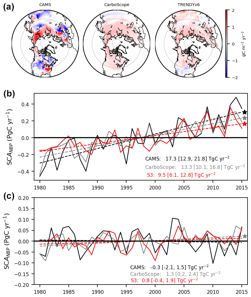
Figure 1Variability in seasonal-cycle amplitude and trends from the inversions and LSMs. (a) Geographical distribution of SCANBP trends from the inversions (CAMS and CarboScope) and the multi-model ensemble mean (MMEM) from TRENDYv6 simulation S3 (all forcings). Both inversions estimated predominantly positive trends in SCANBP>40∘ N (Fig. S1), so we defined two latitudinal bands, L>40 N and L25−40 N, for flux aggregation. (b, c) Aggregated SCANBP time series estimated by the inversions (CAMS in black and CarboScope s76 in grey) and S3 MMEM (red) for L>40 N and L25−40 N, respectively. The dashed lines indicate the linear fits used to calculate the slopes of the trends (corresponding colours), and the slopes and confidence intervals (95 %) are provided.
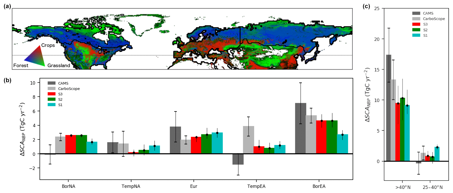
Figure 2Regional distribution of the dominant land-cover types and SCANBP trends. (a) Land-cover map averaged over the study period for the three main land-cover classes (forest–shrubland, grassland and cropland) based on ESA-CCI annual land-cover data (1992–2015 average). (b) The continental regions correspond to the regions defined by Baker et al. (2006) and are delimited by bold lines: boreal and temperate North America (BorNA and TempNA), Europe (Eur), and boreal and temperate Eurasia (BorEA and TempEA). (c) Comparison of the SCANBP trends from the inversions to the trends estimated by the LSM experiments: S3, S2 (no LULCC) and S1 (no LULCC and no climate change). The bars for the inversions and LSMs indicate the average trend over each latitudinal band. The error bars for the inversions indicate the 95 % confidence levels for the trend values, and the vertical lines for the LSMs indicate interquartile ranges of the multi-model ensemble. The 95 % confidence interval for the MMEM was also calculated (see Methods).
The trend in SCANBP was calculated by a least-squares linear fit of annual values for 1980–2015, and confidence intervals were calculated based on Student's t distribution. We tested the robustness of estimated trends of inversions and LSMs for shorter periods by removing the first and last 1–10 years and trends of interannual variability by randomly removing 5 and 10 years of data 104 times. The significance of these trends was calculated using a Mann–Kendall test. We also compared different versions of CarboScope to evaluate the influence of the assimilated network size on the SCANBP trends (Fig. S1). We further calculated the trends for each of the sensitivity tests from CarboScope s85.
3.2 Process attribution
The three TRENDY experiments allow evaluating separately the effects of CO2 fertilization, climate change, and LULCC in the models. The differences between S1 and S2 and between S2 and S3, however, could not isolate specific processes that may have contributed to the trend (e.g. cropland expansion versus afforestation or precipitation versus temperature). Furthermore, the LSMs may miss or simulate certain processes poorly that could influence SCANBP. Therefore, the attribution of drivers by the models is uncertain and should be cross-evaluated. Because inversions do not allow such partitioning between processes, a possible solution is to compare statistical attribution to drivers in inversions and LSMs.
We therefore compared the sensitivity of SCANBP estimated by the inversions and the LSMs by fitting a general linear model (GLM) using the iteratively reweighted least-squares method to eliminate the influence of outliers (Gill, 2000; Green, 1984). We tested the following variables (after unity-based normalization) as predictors: fertilization, irrigation, wood harvest, growing-season precipitation, growing-season temperature, atmospheric CO2 concentration, and change in the extent of cropland and forest. These variables were taken from the corresponding data sets used to force TRENDYv6 models. All possible combinations of n predictors () were tested, and for each value of n, the “best” model (according to Akaike’s information criterion) was chosen separately for each data set. Above n=4 no model showed improved fit compared to the models with fewer predictors. The coefficients from the GLM fit for each data set are shown in Fig. S5.
We further tested the robustness of the statistical relationships by fitting the GLM to the differences between each TRENDYv6 experiment. The significant predictors in the GLM fit to the LSMs in S3 should be detected in the corresponding factorial simulations, e.g. predictors associated with climate should be consistent for the fluxes estimated by the difference between S2 and S1 (effects of climate). The GLM fit to the partial fluxes for the effects of LULCC (S3−S2), climate (S2−S1) and CO2 fertilization (S1−S0) are shown in Fig. S6.
4.1 Large-scale patterns
4.1.1 Top-down estimates
Both inversions estimate increasingly positive trends in SCANBP with increasing latitude, even though CAMS shows heterogeneous patterns in North America, with strong decreasing trends for mid-latitudes (Figs. 1a and S1). Both inversions agree on significant positive SCANBP trends north of 40∘ N (defined here as band L>40 N) and non-significant trends for 25–40∘ N (band L25−40 N; Fig. 1b). In the L>40 N band, CAMS and CarboScope s76 v4.1 estimate an SCANBP increase of 17.3±4.5 and 13.3±3.3 Tg C yr−2, respectively. The uncertainties given for SCANBP trends represent here the uncertainty of the linear fit due to the year-to-year SCANBP variability (Methods). The difference between the CAMS and CarboScope inversions reflects part of the uncertainty in inversions due to their different choices in the ATM (including different atmospheric forcing and spatial resolution), the set of assimilated CO2 data, the prior fluxes, and the a priori spatial and temporal correlation scales and is comparable to the uncertainty of the linear fit due to interannual variability.
This finding is corroborated by two further analyses of inversion uncertainties:
-
While both inversions assimilate atmospheric CO2 measurements from Point Barrow, CAMS increasingly assimilates many other sites in the NH as they become available, helping to better constrain the CO2 fluxes in mid-latitudes to high latitudes with time. Assimilating a non-stationary network of stations, however, possibly leads to spurious additional trends in SCANBP. To test this, we use different runs provided by CarboScope using more sites (but still fixed in number for each run; Fig. S2) for more recent periods. The results from CarboScope version s85 v4.1 (1985–2015) are generally consistent with CAMS, but version s93 v4.1 (1993–2015) estimates much stronger SCANBP trends (Table S1). A higher SCANBP trend in the period 1993–2015 is reported by both CAMS and CarboScope, which estimate very similar trends in L>40 N (19.5 and 19.2 Tg C yr−2, respectively).
-
CarboScope provides a set of sensitivity runs for s85 v4.1, varying some of the inversion's parameters (Fig. S3). Changes in the meteorological fields driving the transport model and the prior ocean fluxes have the largest effect on the SCANBP trends, giving L>40 N trends of 8.6±4.9 Tg C yr−2 (ERA-Interim instead of NCEP) and 13.9±5.6 Tg C yr−2 (fixed ocean), respectively, both well within the uncertainty range (interannual variability affecting linear fit to SCANBP trend) estimated by the standard CarboScope s85 v4.1 (11.7±5.0 Tg C yr−2).
In summary, the ability of inversions to quantify the SCANBP trend is mostly limited by the intrinsic year-to-year SCANBP variability and less so by the amount of information available through the atmospheric data or by inversion settings.
4.1.2 Bottom-up estimates
The large-scale patterns of SCANBP trends from the LSM multi-model ensemble mean (MMEM) of simulation S3 (all forcings) are consistent with CarboScope inversion (Fig. 1a). The MMEM estimates are within the range of the inversions for most latitudes (Fig. S1) but always at the lower end of SCANBP trends reported by inversions. Consistent with inversions, LSMs report a significant trend in L>40 N and a very weak (non-significant) trend in SCANBP in L25−40 N (Fig. 1b). The overall MMEM trend in L>40 N is significantly lower than in inversions (9.5±3.4 Tg C yr−2, i.e. 55 %–71 % of inversions' estimates. The agreement between LSMs and inversions also varies depending on the period and set of inversions considered (LSMs capture 65 %–91 % of inversion trends in 1985–2015 and 74 %–75 % in 1993–2015; Table S1). The MMEM estimate for 1985–2015 (10.6±4.5 Tg C yr−2) is, in fact, even higher than the CarboScope inversion with different meteorological fields (8.6±4.9 Tg C yr−2). These results indicate that, despite a general underestimation of SCANBP trend in L>40 N during 1980–2015 when compared to top-down estimates, the LSMs simulate the main spatiotemporal patterns in SCANBP trends consistent with inversions estimates, especially when accounting for the uncertainty in the latter.
To understand if recent improvements to the set of LSMs and their forcing in TRENDYv6 may have improved their performance in reproducing the SCANBP trend, we compared SCANBP trends from the previous intercomparison round (TRENDYv4). The MMEM from v6 estimates an SCANBP trend in L>40 N that is 43 % higher than in than v4 (MMEM shown in Table S1 but evaluated for individual models). The specific reasons for improvement are hard to identify because of multiple model-dependent changes in the forcing, process simulation and parameterizations from v4 to v6 (Table 4 in Le Quéré et al., 2018).
In summary, we showed that the TRENDYv6 ensemble mean SCANBP trend captures the positive trends in the high latitudes and the lack of trend in the mid-latitudes given by inversions, and underestimates the magnitude of the high latitudes SCANBP trends by 9 %–45 %, depending on the inversion considered and period analysed.
4.2 Regional attribution
The comparison of SCANBP trends in large latitudinal bands may be useful in diagnosing general patterns but is less useful in diagnosing drivers of trends (e.g. climate and agriculture), since ecosystem composition, land management and climate effects are not necessarily separated along a latitudinal gradient. However, the comparison of inversions and models at the pixel scale is also not advisable because the sparse atmospheric network does not allow constraining the fluxes at this scale. We thus compared inversions and LSMs for the SCANBP trends over five sub-continental scale regions: boreal and temperate Eurasian and North American regions and Europe (“TransCom3” regions; Fig. 2). We then use LSMs for attributing SCANBP trends to different drivers using their factorial simulations (Methods).
Inversions and LSMs consistently attribute the increase in SCANBP mainly to boreal Eurasia, both in area-specific (Fig. 1a) and integrated values (Fig. 2b, 5.3–7.1 Tg C yr−2 for inversions and 4.6 Tg C yr−2 for MMEM, respectively), and to Europe (1.9–3.7 and 2.3 Tg C yr−2). The LSMs ascribed the trends in boreal Eurasia approximately equally to climate change and CO2 fertilization (S1 and S2), with LULCC having a slight negative (i.e. decreasing) effect (compare S2 and S3), consistent with the results by Piao et al. (2017). In Europe, LSMs indicate negative contributions from both climate and LULCC. The negative effect of climate may be linked to increasingly drier conditions in this region (Greve et al., 2014) and to strong heatwaves in Europe in the early 21th century (Seneviratne et al., 2012). The negative contribution of LULCC indicated by LSMs in Europe does not support the idea that agricultural intensification or expansion drove an increase in SCANBP and is discussed further on. In temperate Eurasia, inversions disagree on the sign of SCANBP trends, and LSMs indicate weak positive trends dominated by the CO2-fertilization effect. In boreal North America, LSMs estimate SCANBP trends very close to CarboScope estimates, mainly attributed to CO2 followed by climate, whereas CAMS points to a trend close to zero because of cancelling regional trends with opposing sign (Fig. 1a). CAMS and CarboScope point to increasing SCANBP in temperate North America (1.4–1.6 Tg C yr−2), but the LSMs do not indicate any significant change (simulation S3). CAMS (which uses prior information with smaller a priori uncertainties than CarboScope together with a denser network) shows sharper regional differences than CarboScope, which illustrates that there are still substantial differences in the inversion at the scale of continental regions regarding SCANBP trends.
Aggregated over the two latitudinal bands (Fig. 2c), the MMEM indicates a dominant positive effect (increasing SCANBP) of CO2 fertilization both in L25−40 N and L>40 N. In L25−40 N, the CO2 effect is offset by other factors: S1 differs significantly from S2 and S3, which have lower trends of SCANBP. In L>40 N, the MMEM points to a positive effect of climate change in SCANBP trends, thus adding to the CO2 effect. The MMEM suggest a negligible contribution of LULCC to the SCANBP trend in both latitudinal bands. The relative contributions of LULCC, climate and CO2, however, differ between LSMs (Fig. S4). Most models nevertheless agree on non-significant SCANBP trends in L25−40 N as well as on the predominant role of CO2 fertilization and a non-significant contribution of LULCC to the trends in SCANBP in L>40 N. Interestingly, models including carbon–nitrogen interactions had the weakest SCANBP trends (CABLE, ISAM and LPX-Bern), with the exception of CLM4.5, but we cannot draw conclusions from a small set of carbon–nitrogen models.

Figure 3Statistical attribution of drivers of SCANBP estimated by the inversions and LSMs. The main drivers of SCANBP are presented for (a) L>40 N and (b) L25−40 N and are calculated as the product of the coefficients of a general linear model fit on SCANBP using a number of predictors (normalized) and their corresponding trends. Fertilization, irrigation, wood harvest, growing-season precipitation, growing-season temperature and atmospheric CO2 concentration were tested as predictors, and the best fit was chosen for each data set: CAMS (dark grey), CarboScope s76 (light grey) and the MMEM (red). The bars indicate the contribution of each predictor to the trend in SCANBP, error bars indicate the corresponding 95 % confidence intervals and the symbols indicate significant GLM fits (two asterisks, one asterisk and crosses indicate p<0.01, p<0.05 and p<0.1, respectively).
4.3 Driving processes
Figure 3 shows the relative contributions of the predictors (weighted by their trends) found to SCANBP trends in both latitudinal bands. The coefficients of the GLM fit are shown in Fig. S5.
The GLMs provide a better fit the trend of SCANBP in L>40 N (explaining 57 %–74 % of the variance; Table S2) than for L25−40 N (8 %–49 % only). The GLM fit to inversions and to the MMEM identified CO2 fertilization as the most important factor explaining (statistically) the SCANBP trends in both latitudinal bands, consistent with S1 (Figs. 1, S4, S5 and S6), although the CO2-fertilization effect was weaker for the GLM fit to LSMs than for inversions in region L>40 N. The statistical models for inversions and LSMs agreed on a significant negative contribution of warming in both latitudinal bands but a stronger contribution in L25−40 N. GLM models fitted to LSMs and CarboScope also point to changes in forest area contributing to increased SCANBP, and changes in crop area have a negative effect in SCANBP from LSMs. In L25−40 N, the GLM fit to LSMs further points to a small negative contribution of wood harvest to SCANBP trends, and, for CAMS, negative effects of irrigation and fertilization are also significant. The statistical attribution of SCANBP trends in LSMs is generally consistent with the factorial simulations but is mostly clearer for the CO2-fertilization effect than for the other drivers. In the difference between factorial simulations (Fig. S6), some drivers appear to have strong interactive effects, e.g. the effect of CO2 is significantly negative for S3−S2 (LULCC). This could be explained by higher emissions from LULCC under higher CO2 concentrations from the loss of additional sink capacity (Pongratz et al., 2014). The key role of CO2 fertilization in the observed changes is in line with Piao et al. (2017), but our results challenge some of the previously proposed hypotheses to account for the increase in seasonal CO2 exchange, as addressed below.
5.1 Confronting hypotheses
5.1.1 Contribution of LULCC
Agricultural intensification and expansion occurred mainly in latitudes below 45∘ N (Gray et al., 2014), and inversions and LSMs reported instead a peak in the amplitude of land-surface CO2 exchange for latitudes above 45∘ N (Figs. 1 and S1). Furthermore, our regional attribution identifies Eurasia as the region contributing most to increasing SCANBP; this region is dominated by natural ecosystems (Fig. S3) and has experienced very little land use change (Verburg et al., 2015) over the previous decades. Additionally, factorial LSM simulations indicate a negligible contribution of LULCC and management to SCANBP trends not only at the latitudinal-band scale but also regionally (Figs. 1c and 2).
This, though, could not in itself falsify the hypothesis that agricultural intensification is a key driver of SCANBP trends because most LSMs still do not include processes that could intensify cropland NPP over time, such as better cultivars, fertilization and irrigation. Still, management practices are neither a significant predictor for GLM fitted to LSMs nor for inversions, with the exception of CAMS. CarboScope further identifies a negative effect of cropland expansion to SCANBP in L>40 N rather than a positive one, which partly challenges the contribution of cropland expansion (Gray et al., 2014) to SCANBP. Our results are consistent with those by Smith et al. (2014) that show that NPP generally decreased following conversion from natural ecosystems to cropland, except in areas of highly intensive agriculture, such as the midwestern USA. Increasing crop productivity (intensification) could partly explain increasing SCANBP. However, satellite-based data for LAI (Zhu et al., 2016), NPP (Smith et al., 2016) and above-ground biomass (AGB) carbon stocks (Liu et al., 2015) for different land-cover classes from ESA-CCI LC (Fig. S7) indicate that the increase in crop productivity accounted for only a small fraction of the hemispheric trends in ecosystem productivity, consistent with the crop productivity stagnation in Europe and Asia identified by Grassini et al. (2013). We also compared the trends in remote-sensing variables for land-cover classes from LUH2v2h, with similar results.
Previous studies suggesting a large role of the green revolution in SCA trends focused on a longer period, starting in the 1960s. The acceleration of SCANBP reported by inversions and LSMs (Table S1) concurrent with crop productivity stagnation indicates that since the 1980s agriculture intensification is not likely to be the main driver of the increase in SCA. Even in the intensive agricultural areas in the midwestern USA, CAMS estimates contrasting negative and positive trends (Figs. 1a, S8). Eddy-covariance flux measurements (only for 7–13 years) in the areas of intensive agriculture in the USA show a weak relationship between trends in NBP and trends in SCANBP, showing mostly non-significant trends in SCANBP (Fig. S8).
5.1.2 Contribution of warming
We found that warming during the growing season had a negative effect on SCANBP trends in both latitudinal bands, although this effect is uncertain for LSMs in L>40 N. Annual temperature used in the statistical models was also negatively correlated with SCANBP, but the correlation was only significant for CAMS.
The negative relationship with growing-season temperature (T) at the mid-latitudes may be explained by warmer temperature increasing atmospheric demand for water (Novick et al., 2016) and inducing soil-moisture deficits in water-limited regions in summer (Seneviratne et al., 2010) or increased fire risk (Peñuelas et al., 2017) that reduces the summer minimum of SCANBP. This negative effect of temperature can explain the negative contribution of climate to the simulated SCANBP trends in L25−40 N given by the factorial simulations (Fig. 2c).
The negative statistical relationship found between the trend of SCANBP and T in L>40 N challenges the assumption that a warming-related increase in plant productivity in high latitudes necessarily increases the seasonal CO2 exchange (Keeling et al., 1996; Graven et al., 2013; Forkel et al., 2016). Although the MMEM shows a small positive contribution of climate in L>40 N, LSMs diverge on the contribution of climate in this latitudinal band (Fig. S4). Moreover, the factorial simulations in Fig. 2c allow evaluating the impact of changes in all climate variables (e.g. also rainfall and radiation) in addition to temperature. A negative relationship between T and SCA has, though, also been reported by Schneising et al. (2014) for interannual changes in the SCA of total column CO2 for 2004–2010. Yin et al. (2018) have further shown that, at latitudes between 60∘ N and 80∘ N, the relationship between SCA and T has transitioned from positive in the early 1980s to negative in recent decades, reconciling the results by Keeling et al. (1996) and Schneising et al. (2014).
In Fig. S9 we present a conceptual scheme of the impacts of warming in SCANBP through its component fluxes. Generally, warming in high latitudes has been associated with a longer growing season and increased GPP (Piao et al., 2008), which would contribute to increased SCANBP through increased productivity during the “uptake period” and increased decomposition (due to more litter) during the “release period”. However, a weakening of this relationship has been reported (Piao et al., 2014; Peñuelas et al., 2017). Other processes can, though, contribute to the negative relationship between SCANBP and T reported here and in other studies. The empirical negative relationship between trends in SCANBP and warming at the higher latitudes may be due to (i) a stronger effect of T on total ecosystem respiration (TER) than on GPP during the uptake period, (ii) a negative response of ecosystem productivity to warming during the uptake period or (iii) indirect negative effects of T on decomposition during the release period.
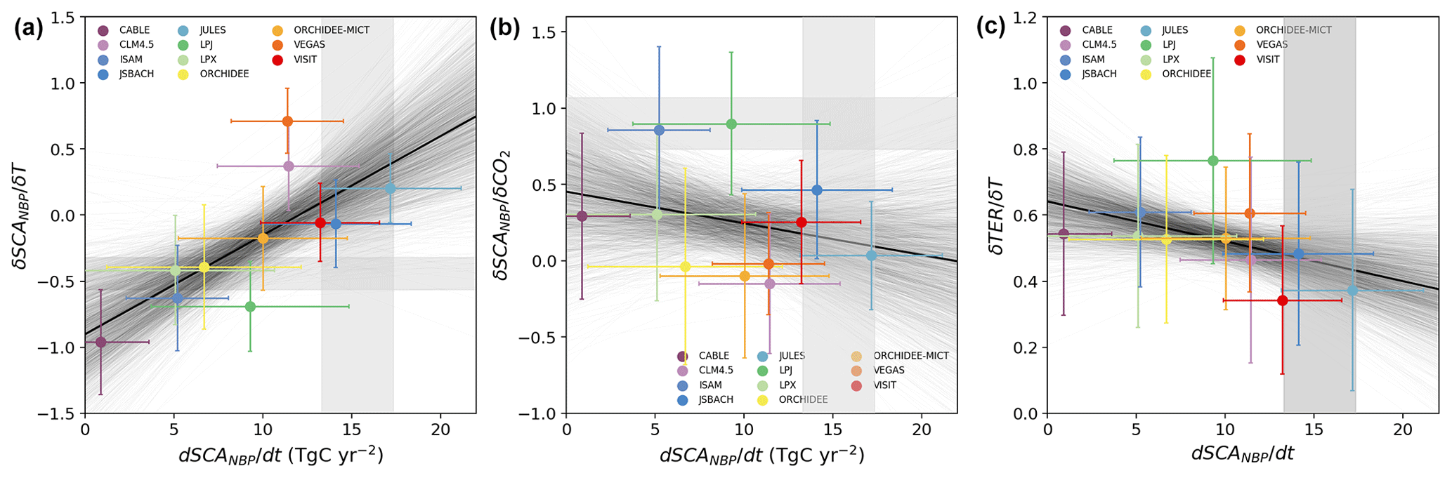
Figure 4Emerging relationships between LSM sensitivities to climate and CO2 and their SCANBP trends. The SCANBP trend for L>40 N estimated by each inversion (grey intervals) and corresponding responses of SCANBP to (a) T and (b) CO2 (as calculated in Fig. 3 but considering the scores of the regression only; shown in Fig. S5) are compared to the results from individual models (simulation S3; coloured markers). In (c) the SCANBP trend for L>40 N estimated by individual models is compared with the simulated sensitivity of TER to T. The shaded areas indicate the inversion ranges, and the distribution of the grey lines shows uncertainty in the relationship between each pair of variables.
Evidence nevertheless supports negative effects of warming on SCA trends. Temperature increase in recent decades has been associated with widespread reduction in the extent and depth of snow cover (Kunkel et al., 2016) and in the number of days with snow cover (Callaghan et al., 2011). Snow has an insulating effect, so snow-covered soil during winter can be kept at relatively constant temperatures, several degrees above the air temperature (>10 ∘C), which promotes respiration of soil C (Nobrega and Grogan, 2007). Soils become subject to more fluctuations in temperature, and become colder, as the snow cover recedes or becomes thinner. Yu et al. (2016) reported that respiration suppression due to a reduction in snow cover in winter may account for as much as 25 % of the increase in the annual CO2 sink of northern forests. A decrease in respiration in response to warming during the release period could thus decrease SCANBP, but the effect of growing-season temperature was stronger in our study. The expansion of vegetation in Arctic tundra, particularly shrubland, has been linked to warming trends but also depends on soil-moisture and permafrost conditions (Elmendorf et al., 2012). Many regions of dry tundra and low arctic shrubland (Walker et al., 2005) experience summer drought or soil-moisture limitations even though northern regions are usually considered to be energy-limited (Greve et al., 2014). Indeed, Myers-Smith et al. (2015) found a strong soil-moisture limitation of the (positive) sensitivity of shrub growth to temperature in summer, possibly associated with the limitation of growth due to drought and/or with reduced growth and dieback due to standing water during thawing. CAMS indicates a decrease in SCANBP in eastern regions in boreal North America (Fig. 1a), where Myers-Smith et al. (2015) reported negative sensitivity of shrub-growth to temperature. The coarse network and large correlation lengths used by CarboScope do not allow such regional contrasts to be resolved. Most process-based models lack a detailed representation of processes described above – e.g. a realistic effect of snow insulation on soil temperatures, soil freezing and thawing (Koven et al., 2009; Peng et al., 2016; Guimberteau et al., 2017) – potentially overestimating the net sink response to temperature changes (Myers-Smith et al., 2015). Moreover, soil-moisture limitation due to temperature increase could also contribute to decreased TER by limiting microbial activity, which is currently not simulated in most LSMs. This may in turn explain why LSMs underestimate the negative effect of temperature in SCANBP in the high latitudes compared to CAMS (Figs. 3 and S4).
5.2 Evaluating model biases
Wenzel et al. (2016) proposed that the observed sensitivity of SCANBP to CO2 was an emergent constraint on future terrestrial photosynthesis, but their study focused on simulations by an earth-system model that excluded the effects of climate change (i.e. the radiative feedback of CO2 to climate was not considered). Our results are consistent with a strong increase in the peak uptake due to the effect of CO2 fertilization driven by GPP as proposed by Wenzel et al. (2016). The negative effect of temperature in our study (Fig. 3), although weaker than the positive effect of absolute CO2 concentration, suggested that warming partly cancelled out the increase in SCANBP expected from the effect of fertilization alone. We propose that other processes partly control SCANBP trends linked to reduced decomposition under lower snow cover (Yu et al., 2016) or to emerging limitations to growth in response to water limitation (Elmendorf et al., 2012; Myers-Smith et al., 2015). Additionally, while the sensitivity of productivity to the CO2-fertilization effect is expected to decrease, the control of respiration by temperature should increase non-linearly (Piao et al., 2014, 2017; Peñuelas et al., 2017), suggesting a progressively dominant (negative) influence of warming on SCANBP. The degree of such an offset would likely depend on the thresholds of soil temperature and water limitation that are complex and thus difficult to assess and require process-based modelling. Our results imply that future constraints of productivity based only on the CO2 effect (as in Wenzel et al., 2016) may overestimate future GPP.
We evaluated whether the differences between the observed SCANBP trends (significant only in L>40 N) and those simulated by the LSMs could be associated with the modelled sensitivities to atmospheric CO2 concentration (CO2) and growing-season temperature (T) in L>40 N (Fig. 4). In Fig. 4, only models with too small a sensitivity of SCANBP to T produce a realistic trend of SCANBP. In contrast, the models indicating sensitivities to T and CO2 more similar to those estimated by the inversions tend to underestimate the trend in SCANBP.
Why are the LSM sensitivities of SCANBP to T positively correlated with their long-term SCANBP trend (Fig. 4) even though CO2 is a stronger driver of the simulated SCANBP trend (Fig. 3)? We found a clear relationship between the model bias in the trend of SCANBP and the sensitivity to CO2 fertilization in S3 (in line with Wenzel et al., 2016), but we also found a compensatory effect, where models that overestimate the sensitivity of SCANBP to T tend to underestimate the sensitivity to CO2 and vice versa. LSMs tend to overestimate the sensitivity of SCANBP to T and underestimate the sensitivity to CO2, compared to the observation-based constraints from inversions. LSMs often compensate too strong (or too weak) a simulated water stress or temperature sensitivity by adjusting photosynthesis parameters (that control CO2 fertilization) during model optimization to match the observed net terrestrial sink. This compensatory effect has previously been reported by Huntzinger et al. (2012) for the mean terrestrial sink; we find that it could also affect the trends in seasonal CO2 exchange.
We argue that the trend of SCANBP can differ between models due to (a) differences in their NPP response to T and CO2, (b) differences in turnover times of short-lived C pools by which increased NPP is coupled to increased winter decomposition, and (c) phase shifts between GPP and ecosystem respiration. These phase shifts may be associated with errors in the phase and amplitude of simulated ecosystem respiration, arising from factors such as (i) representing soil carbon stocks as pools with discrete turnover times and associated effective soil depths (Koven et al., 2009) and (ii) neglect of seasonal acclimation effects on autotrophic and heterotrophic respiration. The sensitivities of NPP to CO2 and T between models are strongly and consistently correlated with the compensatory effect of the model parameterizations (Fig. S10), but we find no clear relationship between the biases of the modelled SCANBP trend and the sensitivity of NPP to T (Fig. S11), suggesting a key role of respiration. Indeed, the models with SCANBP trends closer to observations tend to be associated with a lower sensitivity of ecosystem respiration to growing-season temperature (Fig. S4c). Too large a turnover of short-lived pools in a model should produce too small an increase in the SCANBP amplitude (i.e. increased respiration during the uptake period followed by too little during the release period) for a given sensitivity of NPP to CO2 or climate. A recent study by Jeong et al. (2018) has reported that ecosystem carbon-cycle models (not used in this study) underestimated changes in carbon residence times in northern Alaska. The evaluation of the effect of model turnover times in SCANBP requires a deeper analysis of transfers between litter and soil organic carbon pools and can be verifiable in future simulations.
Based on our assessment of atmospheric observations and the most advanced land-surface model simulations, the most likely explanation of the seasonal cycle of atmospheric CO2 at high latitudes is the CO2 fertilization of photosynthesis in unmanaged high-latitude ecosystems, especially in the Eurasian boreal forests. Our study further points to key processes that need to be developed to better simulate NBP responses to changing climate, especially to Arctic warming, in particular productivity limitations and the decomposition terms. Our results indicated that the signal of the SCANBP trend contains valuable information for the turnover times of short-term pools, which await further investigation.
CAMS v16r1 can be freely available from the COPERNICUS repository: https://apps.ecmwf.int/datasets/data/cams-ghg-inversions/ (last access: 16 November 2017) (Chevallier, 2017). CarboScope s85 v4.1 results are available at http://www.bgc-jena.mpg.de/CarboScope/s/s85_v4.1.html (last access: 26 March 2018) (Rödenbeck, 2017a, b, c) (https://doi.org/10.17871/CarboScope-s85_v4.1, https://doi.org/10.17871/CarboScope-s76_v4.1, and https://doi.org/10.17871/CarboScope-s93_v4.1). LUH2v2h data are freely available at http://gsweb1vh2.umd.edu/LUH2/LUH2_v2h/states.nc (last access: 7 July 2019). ESA-CCI LC maps can be downloaded after registration at http://maps.elie.ucl.ac.be/CCI/viewer/download.php (last access: 1 August 2017). NPP from Smith et al. (2016) can be downloaded from https://drive.google.com/open?id=1m-srVbFoO4IIFGWd__jIoTW7cQEx6890 (last access: 4 August 2017). TRENDYv6 DGVM outputs are available on request to Stephen Sitch (s.a.sitch@exeter.ac.uk) and Pierre Friedlingstein (p.friedlingstein@exeter.ac.uk).
The supplement related to this article is available online at: https://doi.org/10.5194/acp-19-12361-2019-supplement.
AB and PC designed the study, conducted the analysis and wrote the paper. APB, FC, CR, FM, MFM, JP, SLP, WKS, XW, YY and ZZ contributed with expert knowledge during the development of the study. SS and PF coordinated the TRENDY simulations and maintained the TRENDYv6 data. FC and CR developed the atmospheric inversion data sets and contributed to the analysis of inversions. VH, EK, AKJ, SL, DL, JEMSN, PP, BP and DZ performed the TRENDYv6 simulations. All authors contributed to the writing of the paper.
The authors declare that they have no conflict of interest.
This article is part of the special issue “The 10th International Carbon Dioxide Conference (ICDC10) and the 19th WMO/IAEA Meeting on Carbon Dioxide, other Greenhouse Gases and Related Measurement Techniques (GGMT-2017) (AMT/ACP/BG/CP/ESD inter-journal SI)”. It is a result of the 10th International Carbon Dioxide Conference, Interlaken, Switzerland, 21–25 August 2017.
This work was partly supported by the European Space Agency Climate Change Initiative (ESA-CCI) RECCAP-2 project (ESRIN/ 4000123002/18/I-NB). Marcos Fernández-Martinez is a postdoctoral fellow of the Research Foundation – Flanders (FWO). Vanessa Haverd acknowledges support from the Earth Systems and Climate Change Hub, funded by the Australian government's National Environmental Science Program.
This research has been supported by the European Space Agency Climate Change Initiative (RECCAP-2 project (grant no. 4000123002/18/I-NB)).
This paper was edited by Eliza Harris and reviewed by two anonymous referees.
Baker, D. F., Law, R. M., Gurney, K. R., Rayner, P., Peylin, P., Denning, A. S., Bousquet, P., Bruhwiler, L., Chen, Y. H., Ciais, P., Fung, I. Y., Heimann, M., John, J., Maki, T., Maksyutov, S., Masarie, K., Prather, M., Pak, B., Taguchi, S., and Zhu, Z.: TransCom 3 inversion intercomparison: Impact of transport model errors on the interannual variability of regional CO2 fluxes, 1988–2003, Global Biogeochem. Cy., 20, GB1002, https://doi.org/10.1029/2004GB002439, 2006. a, b
Callaghan, T. V., Johansson, M., Brown, R. D., Groisman, P. Y., Labba, N., Radionov, V., Barry, R. G., Bulygina, O. N., Essery, R. L., Frolov, D. M., and Golubev, V. N.: The changing face of Arctic snow cover: A synthesis of observed and projected changes, AMBIO: A Journal of the Human Environment, 40, 17–31, 2011. a
Chevallier, F.: Copernicus Atmosphere Monitoring Service Inversion, available at: https://apps.ecmwf.int/datasets/data/cams-ghg-inversions/, last access: 16 November 2017. a, b
Chevallier, F., Fisher, M., Peylin, P., Serrar, S., Bousquet, P., Bréon, F.-M., Chédin, A., and Ciais, P.: Inferring CO2sources and sinks from satellite observations: Method and application to TOVS data, J. Geophys. Res., 110, D24309, https://doi.org/10.1029/2005jd006390, 2005. a
Chevallier, F., Ciais, P., Conway, T. J., Aalto, T., Anderson, B. E., Bousquet, P., Brunke, E. G., Ciattaglia, L., Esaki, Y., Fröhlich, M., Gomez, A., Gomez-Pelaez, A. J., Haszpra, L., Krummel, P. B., Langenfelds, R. L., Leuenberger, M., Machida, T., Maignan, F., Matsueda, H., MorguÃ, J. A., Mukai, H., Nakazawa, T., Peylin, P., Ramonet, M., Rivier, L., Sawa, Y., Schmidt, M., Steele, L. P., Vay, S. A., Vermeulen, A. T., Wofsy, S., and Worthy, D.: CO2 surface fluxes at grid point scale estimated from a global 21 year reanalysis of atmospheric measurements, J. Geophys. Res., 115, D21307, https://doi.org/10.1029/2010JD013887, 2010. a, b, c
Dargaville, R. J., Heimann, M., McGuire, A. D., Prentice, I. C., Kicklighter, D. W., Joos, F., Clein, J. S., Esser, G., Foley, J., Kaplan, J., and Meier, R. A.: Evaluation of terrestrial carbon cycle models with atmospheric CO2 measurements: Results from transient simulations considering increasing CO2, climate, and land-use effects, Global Biogeochem. Cy., 16, 39-1, 2002. a, b, c
Elmendorf, S. C., Henry, G. H. R., Hollister, R. D., Björk, R. G., Boulanger-Lapointe, N., Cooper, E. J., Cornelissen, J. H. C., Day, T. A., Dorrepaal, E., and Elumeeva, T. G.: Plot-scale evidence of tundra vegetation change and links to recent summer warming, Nat. Clim. Change, 2, 453–457, 2012. a, b
Forkel, M., Carvalhais, N., Rödenbeck, C., Keeling, R., Heimann, M., Thonicke, K., Zaehle, S., and Reichstein, M.: Enhanced seasonal CO2 exchange caused by amplified plant productivity in northern ecosystems, Science, 351, 696–699, 2016. a, b, c
Gill, J.: Generalized linear models: a unified approach, vol. 134, Sage Publications, Thousand Oaks, 91320 California, USA, 2000. a
Grassini, P., Eskridge, K. M., and Cassman, K. G.: Distinguishing between yield advances and yield plateaus in historical crop production trends, Nat. Commun., 4, 2918, 2013. a, b
Graven, H. D., Keeling, R. F., Piper, S. C., Patra, P. K., Stephens, B. B., Wofsy, S. C., Welp, L. R., Sweeney, C., Tans, P. P., Kelley, J. J., Daube, B. C., Kort, E. A., Santoni, G. W., and Bent, J. D.: Enhanced Seasonal Exchange of CO2 by Northern Ecosystems Since 1960, Science, 341, 1085–1089, 2013. a, b, c
Gray, J. M., Frolking, S., Kort, E. A., Ray, D. K., Kucharik, C. J., Ramankutty, N., and Friedl, M. A.: Direct human influence on atmospheric CO2 seasonality from increased cropland productivity, Nature, 515, 398–401, https://doi.org/10.1038/nature13957, 2014. a, b, c
Green, P. J.: Iteratively reweighted least squares for maximum likelihood estimation, and some robust and resistant alternatives, J. R. Stat. Soc. B, 46, 149–192, 1984. a
Greve, P., Orlowsky, B., Mueller, B., Sheffield, J., Reichstein, M., and Seneviratne, S. I.: Global assessment of trends in wetting and drying over land, Nat. Geosci., 7, 716–721, 2014. a, b
Guimberteau, M., Zhu, D., Maignan, F., Huang, Y., Yue, C., Dantec-Nédélec, S., Ottlé, C., Jornet-Puig, A., Bastos, A., Laurent, P., Goll, D., Bowring, S., Chang, J., Guenet, B., Tifafi, M., Peng, S., Krinner, G., Ducharne, A., Wang, F., Wang, T., Wang, X., Wang, Y., Yin, Z., Lauerwald, R., Joetzjer, E., Qiu, C., Kim, H., and Ciais, P.: ORCHIDEE-MICT (v8.4.1), a land surface model for the high latitudes: model description and validation, Geosci. Model Dev., 11, 121–163, https://doi.org/10.5194/gmd-11-121-2018, 2018. a
Harris, I., Jones, P. D., Osborn, T. J., and Lister, D. H.: Updated high-resolution grids of monthly climatic observations – the CRU TS3. 10 Dataset, Int. J. Climatol., 34, 623–642, 2014. a
Huntzinger, D. N., Post, W. M., Wei, Y., Michalak, A. M., West, T. O., Jacobson, A. R., Baker, I. T., Chen, J. M., Davis, K. J., Hayes, D. J., and Hoffman, F. M.: North American Carbon Program (NACP) regional interim synthesis: Terrestrial biospheric model intercomparison, Ecol. Modell., 232, 144–157, 2012. a
Hurtt, G. C., Chini, L. P., Frolking, S., Betts, R. A., Feddema, J., Fischer, G., Fisk, J. P., Hibbard, K., Houghton, R. A., Janetos, A., and Jones, C. D.: Harmonization of land-use scenarios for the period 1500–2100: 600 years of global gridded annual land-use transitions, wood harvest, and resulting secondary lands, Clim. Change, 109, 117–161, 2011. a, b
Jeong, S. J., Bloom, A. A., Schimel, D., Sweeney, C., Parazoo, N. C., Medvigy, D., Schaepman-Strub, G., Zheng, C., Schwalm, C. R., Huntzinger, D. N., and Michalak, A. M.: Accelerating rates of Arctic carbon cycling revealed by long-term atmospheric CO2 measurements, Sci. Adv., 4, eaao1167, https://doi.org/10.1126/sciadv.aao1167, 2018. a
Kaminski, T. and Heimann, M.: Inverse Modeling of Atmospheric Carbon Dioxide Fluxes, Science, 294, 259–259, 2001. a
Keeling, C. D., Chin, J. F. S., and Whorf, T. P.: Increased activity of northern vegetation inferred from atmospheric CO2 measurements, Nature, 382, 146–149, https://doi.org/10.1038/382146a0, 1996. a, b, c
Koven, C., Friedlingstein, P., Ciais, P., Khvorostyanov, D., Krinner, G., and Tarnocai, C.: On the formation of high-latitude soil carbon stocks: Effects of cryoturbation and insulation by organic matter in a land surface model, Geophys. Res. Lett., 36, L21501, https://doi.org/10.1029/2009GL040150, 2009. a, b
Kunkel, K. E., Robinson, D. A., Champion, S., Yin, X., Estilow, T., and Frankson, R. M.: Trends and extremes in Northern Hemisphere snow characteristics, Current Climate Change Reports, 2, 65–73, 2016. a
Le Quéré, C., Andrew, R. M., Friedlingstein, P., Sitch, S., Pongratz, J., Manning, A. C., Korsbakken, J. I., Peters, G. P., Canadell, J. G., Jackson, R. B., Boden, T. A., Tans, P. P., Andrews, O. D., Arora, V. K., Bakker, D. C. E., Barbero, L., Becker, M., Betts, R. A., Bopp, L., Chevallier, F., Chini, L. P., Ciais, P., Cosca, C. E., Cross, J., Currie, K., Gasser, T., Harris, I., Hauck, J., Haverd, V., Houghton, R. A., Hunt, C. W., Hurtt, G., Ilyina, T., Jain, A. K., Kato, E., Kautz, M., Keeling, R. F., Klein Goldewijk, K., Körtzinger, A., Landschützer, P., Lefèvre, N., Lenton, A., Lienert, S., Lima, I., Lombardozzi, D., Metzl, N., Millero, F., Monteiro, P. M. S., Munro, D. R., Nabel, J. E. M. S., Nakaoka, S., Nojiri, Y., Padin, X. A., Peregon, A., Pfeil, B., Pierrot, D., Poulter, B., Rehder, G., Reimer, J., Rödenbeck, C., Schwinger, J., Séférian, R., Skjelvan, I., Stocker, B. D., Tian, H., Tilbrook, B., Tubiello, F. N., van der Laan-Luijkx, I. T., van der Werf, G. R., van Heuven, S., Viovy, N., Vuichard, N., Walker, A. P., Watson, A. J., Wiltshire, A. J., Zaehle, S., and Zhu, D.: Global Carbon Budget 2017, Earth Syst. Sci. Data, 10, 405–448, https://doi.org/10.5194/essd-10-405-2018, 2018. a, b, c, d
Liu, Y. Y., Van Dijk, A. I., De Jeu, R. A., Canadell, J. G., McCabe, M. F., Evans, J. P., and Wang, G.: Recent reversal in loss of global terrestrial biomass, Nat. Clim. Change, 5, 470–474, 2015. a, b
Myers-Smith, I. H., Elmendorf, S. C., Beck, P. S., Wilmking, M., Hallinger, M., Blok, D., Tape, K. D., Rayback, S. A., Macias-Fauria, M., Forbes, B. C., and Speed, J. D.: Climate sensitivity of shrub growth across the tundra biome, Nat. Clim. Change, 5, 887–891, 2015. a, b, c, d
Nobrega, S. and Grogan, P.: Deeper snow enhances winter respiration from both plant-associated and bulk soil carbon pools in birch hummock tundra, Ecosystems, 10, 419–431, 2007. a
Novick, K. A., Ficklin, D. L., Stoy, P. C., Williams, C. A., Bohrer, G., Oishi, A., Papuga, S. A., Blanken, P. D., Noormets, A., Sulman, B. N., Scott, R. L., Wang, L., and Phillips, R. P.: The increasing importance of atmospheric demand for ecosystem water and carbon fluxes, Nat. Clim. Change, 6, 1023, https://doi.org/10.1038/nclimate3114, 2016. a
Peng, S., Ciais, P., Krinner, G., Wang, T., Gouttevin, I., McGuire, A. D., Lawrence, D., Burke, E., Chen, X., Decharme, B., Koven, C., MacDougall, A., Rinke, A., Saito, K., Zhang, W., Alkama, R., Bohn, T. J., Delire, C., Hajima, T., Ji, D., Lettenmaier, D. P., Miller, P. A., Moore, J. C., Smith, B., and Sueyoshi, T.: Simulated high-latitude soil thermal dynamics during the past 4 decades, The Cryosphere, 10, 179–192, https://doi.org/10.5194/tc-10-179-2016, 2016. a
Peñuelas, J., Ciais, P., Canadell, J. G., Janssens, I. A., Fernández-Martínez, M., Carnicer, J., Obersteiner, M., Piao, S., Vautard, R., and Sardans, J.: Shifting from a fertilization-dominated to a warming-dominated period, Nature Ecology Evolution, 1, 1438–1445, 2017. a, b, c
Peylin, P., Law, R. M., Gurney, K. R., Chevallier, F., Jacobson, A. R., Maki, T., Niwa, Y., Patra, P. K., Peters, W., Rayner, P. J., Rödenbeck, C., van der Laan-Luijkx, I. T., and Zhang, X.: Global atmospheric carbon budget: results from an ensemble of atmospheric CO2 inversions, Biogeosciences, 10, 6699–6720, https://doi.org/10.5194/bg-10-6699-2013, 2013. a
Piao, S., Ciais, P., Friedlingstein, P., Peylin, P., Reichstein, M., Luyssaert, S., Margolis, H., Fang, J., Barr, A., Chen, A., Grelle, A., Hollinger, D. Y., Laurila, T., Lindroth, A., Richardson, A. D., and Vesala, T.: Net carbon dioxide losses of northern ecosystems in response to autumn warming, Nature, 451, 49–52, https://doi.org/10.1038/nature06444, 2008. a
Piao, S., Nan, H., Huntingford, C., Ciais, P., Friedlingstein, P., Sitch, S., Peng, S., Ahlström, A., Canadell, J. G., Cong, N., Levis, S., Levy, P. E., Liu, L., Lomas, M. R., Mao, J., Myneni, R. B., Peylin, P., Poulter, B., Shi, X., Yin, G., Viovy, N., Wang, T., Wang, X., Zaehle, S., Zeng, N., Zeng, Z., and Chen, A.: Evidence for a weakening relationship between interannual temperature variability and northern vegetation activity, Nat. Commun., 5, 5018, https://doi.org/10.1038/ncomms6018, 2014. a, b
Piao, S., Liu, Z., Wang, Y., Ciais, P., Yao, Y., Peng, S., Chevallier, F., Friedlingstein, P., Janssens, I. A., Peñuelas, J., and Sitch, S.: On the causes of trends in the seasonal amplitude of atmospheric CO2, Global change biology, Glob. Change Biol., 24, 608–616, 2017. a, b, c, d, e, f, g, h, i
Pongratz, J., Reick, C. H., Houghton, R. A., and House, J. I.: Terminology as a key uncertainty in net land use and land cover change carbon flux estimates, Earth Syst. Dynam., 5, 177–195, https://doi.org/10.5194/esd-5-177-2014, 2014. a
Rödenbeck, C.: Estimating CO2 sources and sinks from atmospheric mixing ratio measurements using a global inversion of atmospheric transport, Technical Report 6, Max Planck Institute for Biogeochemistry, 07701 Jena, Germany, 2005. a, b, c
Rödenbeck, C.: Atmospheric CO2 Inversion, 1985–2016, https://doi.org/10.17871/CarboScope-s85_v4.1, 2017a. a
Rödenbeck, C.: Atmospheric CO2 Inversion, 1976–2016, https://doi.org/10.17871/CarboScope-s76_v4.1, 2017b. a
Rödenbeck, C.: Atmospheric CO2 Inversion, 1993–2016, https://doi.org/10.17871/CarboScope-s93_v4.1, 2017c. a
Rödenbeck, C., Houweling, S., Gloor, M., and Heimann, M.: CO2 flux history 1982–2001 inferred from atmospheric data using a global inversion of atmospheric transport, Atmos. Chem. Phys., 3, 1919–1964, https://doi.org/10.5194/acp-3-1919-2003, 2003. a
Schneising, O., Reuter, M., Buchwitz, M., Heymann, J., Bovensmann, H., and Burrows, J. P.: Terrestrial carbon sink observed from space: variation of growth rates and seasonal cycle amplitudes in response to interannual surface temperature variability, Atmos. Chem. Phys., 14, 133–141, https://doi.org/10.5194/acp-14-133-2014, 2014. a, b
Seneviratne, S. I., Corti, T., Davin, E. L., Hirschi, M., Jaeger, E. B., Lehner, I., Orlowsky, B., and Teuling, A. J.: Investigating soil moisture–climate interactions in a changing climate: A review, Earth-Sci. Rev., 99, 125–161, 2010. a
Seneviratne, S. I., Nicholls, N., Easterling, D., Goodess, C., Kanae, S., Kossin, J., Luo, Y., Marengo, J., McInnes, K., and Rahimi, M.: Changes in climate extremes and their impacts on the natural physical environment, Managing the risks of extreme events and disasters to advance climate change adaptation, in: Managing the risks of extreme events and disasters to advance climate change adaptation: Special report of the Intergovernmental Panel on Climate Change, 109–230, Cambridge University Press, pp. 109–230, 2012. a
Sitch, S., Friedlingstein, P., Gruber, N., Jones, S. D., Murray-Tortarolo, G., Ahlström, A., Doney, S. C., Graven, H., Heinze, C., Huntingford, C., Levis, S., Levy, P. E., Lomas, M., Poulter, B., Viovy, N., Zaehle, S., Zeng, N., Arneth, A., Bonan, G., Bopp, L., Canadell, J. G., Chevallier, F., Ciais, P., Ellis, R., Gloor, M., Peylin, P., Piao, S. L., Le Quéré, C., Smith, B., Zhu, Z., and Myneni, R.: Recent trends and drivers of regional sources and sinks of carbon dioxide, Biogeosciences, 12, 653–679, https://doi.org/10.5194/bg-12-653-2015, 2015. a
Smith, W. K., Cleveland, C. C., Reed, S. C., and Running, S. W.: Agricultural conversion without external water and nutrient inputs reduces terrestrial vegetation productivity, Geophys. Res. Lett., 41, 449–455, 2014. a
Smith, W. K., Reed, S. C., Cleveland, C. C., Ballantyne, A. P., Anderegg, W. R., Wieder, W. R., Liu, Y. Y., and Running, S. W.: Large divergence of satellite and Earth system model estimates of global terrestrial CO2 fertilization, Nat. Clim. Change, 6, 306–310, 2016. a, b
Thomas, R. T., Prentice, I. C., Graven, H., Ciais, P., Fisher, J. B., Hayes, D. J., Huang, M., Huntzinger, D. N., Ito, A., Jain, A., and Mao, J.: Increased light-use efficiency in northern terrestrial ecosystems indicated by CO2 and greening observations, Geophys. Res. Lett., 43, 11339–11349, 2016. a, b, c
Verburg, P. H., Crossman, N., Ellis, E. C., Heinimann, A., Hostert, P., Mertz, O., Nagendra, H., Sikor, T., Erb, K. H., Golubiewski, N., and Grau, R.: Land system science and sustainable development of the earth system: A global land project perspective, Anthropocene, 12, 29–41, 2015. a
Viovy, N.: CRUNCEP data set, available at: ftp://nacp.ornl.gov/synthesis/2009/frescati/temp/land_use_change/original/readme.htm (last access: 27 July 2017), 2016. a
Walker, D. A., Raynolds, M. K., Daniëls, F. J., Einarsson, E., Elvebakk, A., Gould, W. A., Katenin, A. E., Kholod, S. S., Markon, C. J., Melnikov, E. S., and Moskalenko, N. G.: The circumpolar Arctic vegetation map, J. Veg. Sci., 16, 267–282, 2005. a
Welp, L. R., Patra, P. K., Rödenbeck, C., Nemani, R., Bi, J., Piper, S. C., and Keeling, R. F.: Increasing summer net CO2 uptake in high northern ecosystems inferred from atmospheric inversions and comparisons to remote-sensing NDVI, Atmos. Chem. Phys., 16, 9047–9066, https://doi.org/10.5194/acp-16-9047-2016, 2016. a
Wenzel, S., Cox, P. M., Eyring, V., and Friedlingstein, P.: Projected land photosynthesis constrained by changes in the seasonal cycle of atmospheric CO2, Nature, 538, 499–501, 2016. a, b, c, d
Yin, Y., Ciais, P., Chevallier, F., Li, W., Bastos, A., Piao, S., Wang, T., and Liu, H.: Changes in the response of the Northern Hemisphere carbon uptake to temperature over the last three decades, Geophys. Res. Lett., 45, 4371–4380, 2018. a, b
Yu, Z., Wang, J., Liu, S., Piao, S., Ciais, P., Running, S. W., Poulter, B., Rentch, J. S., and Sun, P.: Decrease in winter respiration explains 25% of the annual northern forest carbon sink enhancement over the last 30 years, Global Ecol. Biogeogr., 25, 586–595, 2016. a, b
Zeng, N., Zhao, F., Collatz, G. J., Kalnay, E., Salawitch, R. J., West, T. O., and Guanter, L.: Agricultural Green Revolution as a driver of increasing atmospheric CO2 seasonal amplitude, Nature, 515, 394–397, https://doi.org/10.1038/nature13893, 2014. a
Zhu, D., Peng, S. S., Ciais, P., Viovy, N., Druel, A., Kageyama, M., Krinner, G., Peylin, P., Ottlé, C., Piao, S. L., Poulter, B., Schepaschenko, D., and Shvidenko, A.: Improving the dynamics of Northern Hemisphere high-latitude vegetation in the ORCHIDEE ecosystem model, Geosci. Model Dev., 8, 2263–2283, https://doi.org/10.5194/gmd-8-2263-2015, 2015. a
Zhu, Z., Piao, S., Myneni, R. B., Huang, M., Zeng, Z., Canadell, J. G., Ciais, P., Sitch, S., Friedlingstein, P., Arneth, A., and Cao, C.: Greening of the Earth and its drivers, Nat. Clim. Change, 6, 791–795, 2016. a