the Creative Commons Attribution 4.0 License.
the Creative Commons Attribution 4.0 License.
 | 07 Oct 2019
Relative impact of aerosol, soil moisture, and orography perturbations on deep convection
Linda Schneider
Christian Barthlott
Corinna Hoose
Andrew I. Barrett
The predictability of deep moist convection depends on many factors, such as the synoptic-scale flow, the geographical region (i.e., the presence of mountains), and land surface–atmosphere as well as aerosol–cloud interactions. This study addresses all these factors by investigating the relative impact of orography, soil moisture, and aerosols on precipitation over Germany in different weather regimes. To this end, we conduct numerical sensitivity studies with the COnsortium for Small-sale MOdelling (COSMO) model at high spatial resolution (500 m grid spacing) for 6 days with weak and strong synoptic forcing. The numerical experiments consist of (i) successive smoothing of topographical features, (ii) systematic changes in the initial soil moisture fields (spatially homogeneous increase/decrease, horizontal uniform soil moisture, different realizations of dry/wet patches), and (iii) different assumptions about the ambient aerosol concentration (spatially homogeneous and heterogeneous fields). Our results show that the impact of these perturbations on precipitation is on average higher for weak than for strong synoptic forcing. Soil moisture and aerosols are each responsible for the maximum precipitation response for three of the cases, while the sensitivity to terrain forcing always shows the smallest spread. For the majority of the analyzed cases, the model produces a positive soil moisture–precipitation feedback when averaged over the entire model domain. Furthermore, the amount of soil moisture affects precipitation more strongly than its spatial distribution. The precipitation response to changes in the CCN concentration is more complex and case dependent. The smoothing of terrain shows weaker impacts on days with strong synoptic forcing because surface fluxes are less important and orographic ascent is still simulated reasonably well, despite missing fine-scale orographic features. We apply an object-based characterization to identify whether and how the perturbations affect the structure, location, timing, and intensity of precipitation. These diagnostics reveal that the structure component, comparing the size and shape of precipitating objects to the reference simulation, is on average highest in the soil moisture and aerosol simulations, often due to changes in the maximum precipitation amounts. This indicates that the dominant mechanisms for convection initiation remain but that precipitation amounts depend on the strength of the trigger mechanisms. Location and amplitude parameters both vary over a much smaller range. Still, the temporal evolution of the amplitude component correlates well with the rain rate. Our results suggest that for quantitative precipitation forecasting, both aerosols and soil moisture are of similar importance and that their inclusion in convective-scale ensemble forecasting containing classical sources of uncertainty should be assessed in the future.
- Article
(18029 KB) - Full-text XML
- BibTeX
- EndNote


Forecasting convective precipitation remains one of the key challenges in numerical weather prediction (NWP) and has large social, economic, and environmental impacts due to the multiple risks from hail, lightning, strong winds, and heavy precipitation. Convective precipitation results from a chain of complex processes and multi-scale interactions in the atmosphere and is therefore accompanied by numerous uncertainties in its formation. Although convection-permitting models have provided a step change in rainfall forecasting capabilities (Clark et al., 2016), current state-of-the art models still exhibit persistent and systematic shortcomings due to an inadequate representation of unresolved processes (Berner et al., 2017). This makes it difficult to properly predict convective precipitation, resulting in an often inadequate accuracy for many applications (Kühnlein et al., 2014; Mittermaier, 2014). The predictability of convective precipitation, i.e., the degree to which a correct prediction of the state of the atmosphere can be made, depends on many aspects, such as, among others, the synoptic-scale flow, the geographical region (i.e., the presence of mountains), the underlying land surface, and microphysical conditions. For thermally forced convection, physical understanding is further challenged by the essential nonlinearity of thermally driven circulations, large spatial heterogeneity in thermodynamics and winds over complex terrain, and multi-scale interactions between the land surface and the planetary boundary layer (e.g., Kirshbaum et al., 2018; Groenemeijer et al., 2009). Land surface properties (e.g., land cover, terrain, and soil texture) are highly heterogeneous across a wide range of spatiotemporal scales (Santanello et al., 2018) and potential linkages between land surface variables and atmospheric variables such as temperature and precipitation are difficult to establish (e.g., Seneviratne et al., 2010). Over mountainous terrain, thermally induced wind systems and low-level convergence zones are crucial for the initiation of deep convection with prevailing weak winds (e.g., Schneider et al., 2018). They are often less well resolved in operational models, which limits the forecast capabilities, in contrast to situations governed by large-scale synoptic forcing, when the forecast of precipitation is often more reliable (Baldauf et al., 2011). Previous studies have shown that the knowledge of the orographically modified flow is essential to predict intensity, location, and duration of precipitation (e.g., Rotunno and Ferretti, 2001; Rotunno and Houze, 2007; Barthlott et al., 2016).
The relevance of soil moisture for convective precipitation has been investigated in many studies (e.g., Schär et al., 1999; Findell and Eltahir, 2003; Seneviratne et al., 2010; Richard et al., 2011). Despite a robust understanding that higher soil moisture leads to an increase in the near-surface specific humidity and a decrease in temperature, the soil moisture–precipitation feedback is highly complex and may vary spatially and temporarily (Pan et al., 1996). Furthermore, soil moisture contents in models often show large differences to observations (Hauck et al., 2011). The initial soil moisture content can be of large importance as well: for a case study, Barthlott and Kalthoff (2011) showed that for drier soils (where evaporation is controlled by soil moisture), a systematic positive soil moisture–precipitation feedback exists, whereas for already quite wet soils (where evapotranspiration is controlled by net radiation), the influence of increasing soil moisture is much weaker and the general response of precipitation to soil moisture is not systematic anymore. Additionally, the presence of horizontal land surface wetness gradients, which induce gradients in the sensible heat flux, can foster mesoscale circulations, resulting in more precipitation over dry soils (Taylor et al., 2012). A negative soil moisture–precipitation feedback was also found for convection-resolving simulations by Hohenegger et al. (2009). In their simulations, dry initial soil moisture conditions yield more vigorous thermals (owing to stronger daytime heating), which can more easily break through stable air barriers above, thereby leading to deep convection and ultimately to a negative soil moisture–precipitation feedback loop. Moreover, the strength of the background wind was found to change precipitation patterns even more (Froidevaux et al., 2014; Guillod et al., 2014), leading to a non-systematic soil moisture–precipitation feedback.
Besides the unclear roles of the underlying terrain and the soil moisture–precipitation feedback in different weather regimes, there are large uncertainties arising from the nonlinear character of the microphysics and the complexity of the microphysical system with many possible process pathways (Seifert et al., 2012). Many recent studies documented that the response of clouds to changes in the aerosol concentration is complex and may differ depending on the cloud type or aerosol regime or environmental conditions (e.g., Khain et al., 2008; Noppel et al., 2010; van den Heever et al., 2011; Barthlott and Hoose, 2018) and may be complicated by processes below clouds, such as evaporation (e.g., Barthlott et al., 2017). Moreover, the validity of the invigoration hypothesis (Rosenfeld et al., 2008) in polluted conditions (i.e., updraft invigoration by additional latent heating due to a larger water load above the freezing level) and the possibility of climate responses to this effect are still considered to be open questions (Altaratz et al., 2014).
Ensemble forecasting has become a standard tool for probabilistic numerical weather prediction, and most major meteorological services now run such systems routinely (e.g., Bouttier and Raynaud, 2018). Key uncertainties that are accounted for comprise, e.g., the uncertainties in the initial and lateral boundary conditions as well as uncertainties in the representation of physical processes (e.g., Clark et al., 2016, and references therein). To address predictability thoroughly, relevant sources of uncertainty need to be identified. While terrain forcing, soil moisture, and aerosol impacts on convective precipitation have been investigated separately in many studies, the relative effect of these perturbations for the same weather situations has not been investigated so far. Up to now, there exist only studies with idealized simulations on the isolated and collective effects of terrain and soil moisture heterogeneity. Rihani et al. (2015) conducted large-eddy simulations and found that terrain effects dominate the planetary boundary layer development during early morning hours, while the soil moisture signature overcomes that of terrain during the afternoon. With convection-resolving simulations, Imamovic et al. (2017) found a consistently positive soil moisture–precipitation feedback for horizontally uniform perturbations, irrespective of the presence of low orography. However, a negative feedback emerged with localized perturbations. In both of these studies, terrain modifications were much more extensive via flattening of the idealized mountains. Moreover, uncertainties of the aerosol load were not addressed. Thus, the aim of this study is to investigate the uncertainties that variations in orography, soil moisture, and aerosols impose on convective precipitation by means of real-case simulations. To cover different weather regimes typical for central Europe, we analyze days with weak large-scale forcing (air-mass convection) and strong large-scale forcing (passage of frontal zones). This study is unique as it is the first (to the best of our knowledge) to address the relative impacts of these uncertainties on convective-scale predictability. It is of general relevance to assess to which extent these uncertainties should be considered in future convective-scale ensemble forecasting systems.
2.1 Numerical model
The general model setup follows the one from Schneider et al. (2018). All simulations were conducted with version 5.3 of the COnsortium for Small-sale MOdelling (COSMO) model (Schättler et al., 2016). It is a non-hydrostatic limited-area atmospheric prediction model, which operates on a rotated latitude–longitude grid with an Arakawa C-grid for horizontal differencing. First, simulations are performed with 2.8 km grid spacing on the operational COSMO-DE grid of the German Weather Service driven by 7 km COSMO-EU initial and boundary data (see Schneider et al., 2018, for the exact domain location). The model uses terrain-following coordinates and 50 levels in the vertical. The time integration is realized using a two-time-level Runge–Kutta method (Wicker and Skamarock, 2002); the time step is set to 25 s. Whereas deep convection is fully resolved, shallow convection is parameterized with a modified Tiedtke scheme with moisture-convergence closure (Tiedtke, 1989). Shallow convection is limited to a cloud depth of 250 hPa and is non-precipitating (see Baldauf et al., 2011, and Theunert and Seifert, 2006, for details). We use a 1-D turbulence scheme, which is based on a prognostic equation for the turbulent kinetic energy and which can be classified as Mellor–Yamada level 2.5 (Mellor and Yamada, 1974). The model further includes a multilayer soil vegetation model, TERRA-ML (Doms et al., 2011), with six soil levels. In contrast to the operationally used setup, we use the two-moment microphysics scheme of Seifert and Beheng (2006) to represent aerosol effects on the microphysics of mixed-phase clouds. The two-moment scheme predicts the mass and number concentration of six different hydrometeors (cloud water, rain, cloud ice, graupel, snow, and hail) and allows us to use different constant cloud condensation nuclei (CCN) concentration assumptions. The preprocessing of the initial and boundary data is done with the INT2LM preprocessor (Schättler and Blahak, 2017).
Then, a 500 m grid is nested into the 2.8 km domain using one-way interfaces (Fig. 1a). Such a fine grid resolution was also used in COSMO simulations exploring the gray zone by Barthlott and Hoose (2015). They showed several benefits compared to coarser resolutions, such as a better representation of low-level convergence zones or gravity waves. The domain size is reduced, covering approximately 750 km×700 km (1510×1300 grid points), and spans almost the whole of Germany.
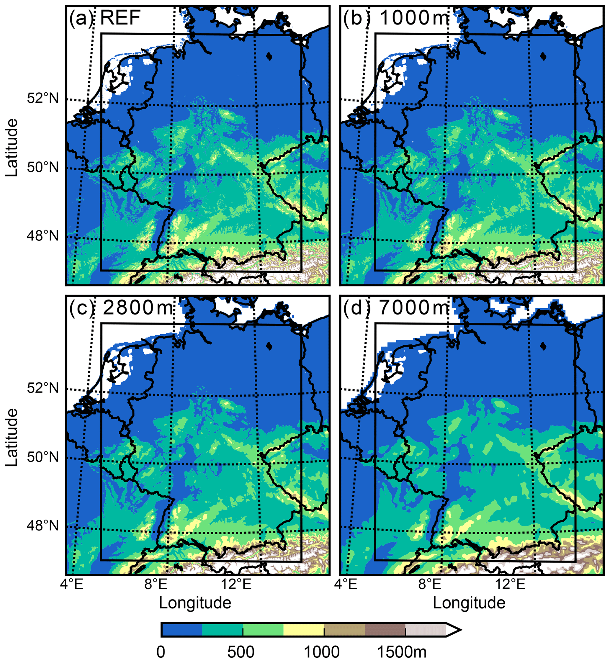
Figure 1Reference orography at 500 m grid spacing (a) and interpolated orography from 1 km (b), 2.8 km (c), and 7 km (d) to the model grid. The black rectangle depicts the 500 m simulation domain.
The number of vertical levels is increased to 80, with 18 levels in the lowest kilometer. Deep as well as shallow convection are now fully resolved and the Tiedtke schemes for shallow and deep convection are both switched off. Instead of a 1-D boundary-layer approximation, turbulence is now parameterized with a 3-D closure, where both vertical and horizontal turbulent diffusion is active (Doms et al., 2011). The time step is reduced to 3 s for numerical stability. For this reference run, we use a continental aerosol assumption with a number density of 1700 cm−3 typical for central Europe (Hande et al., 2016). All simulations had an integration time of 24 h. Spin-up effects (e.g., increased wind convergence or weak isolated rain) are only simulated during the first 2–3 h of integration time, which do not affect the subsequent precipitation discussed herein.
2.2 Sensitivity studies
To address the relative impacts of land surface and aerosol heterogeneities on deep convection, we perform several numerical sensitivity studies which are summarized in Table 1.
Table 1Overview of the performed numerical sensitivity simulations. The reference run and all orography/soil moisture perturbations use a continental CCN assumption (CON). The relative soil moisture content wso is modified only at model initialization.

The successive smoothing of individual terrain features is realized by taking external parameters (terrain height, land use, roughness length, etc.) at coarser resolution (1, 2.8, and 7 km), which are then interpolated onto the 500 m model grid (hereafter referred to as EXT1000, EXT2800, and EXT7000). This results in somewhat lower mountain top heights and less well-resolved valleys (Fig. 1). Such a technique was also applied by Schumacher et al. (2015) for studying banded convection in the lee of the Rocky Mountains and Picard and Mass (2017) for investigating the impact of the flow direction on orographic precipitation over the US Pacific Northwest.

Figure 2Relative water content of the reference field (REF, a), the simulations with small (SM_RS, b) and medium (SM_RM, c) random structures, and chessboard structures with grid lengths of 10 km (SM_10k, d), 56 km (SM_56k, e), and 112 km (SM_112k, f).
The majority of the sensitivity runs in this study consist of different soil moisture assumptions (Fig. 2). First, a simulation with spatially homogeneous soil moisture is performed (SM_UNI), assuming for every grid point the domain-averaged relative water content . The relative water content is computed at each grid point from the volumetric water content (VWC) and the soil-type-dependent wilting point (WP) and porosity (PO) as follows:
Thus, there are no horizontal soil moisture gradients. Then, we introduce a positive and negative soil moisture bias by increasing (SM_125) or decreasing (SM_075) the initial soil moisture field by 25 % at every grid point. The value of 25 % was selected because Hauck et al. (2011) showed that simulated and observed soil moisture in southwestern Germany differs around 20 %–30 %. Chessboard structures are implemented with grid lengths of 10 km (SM_10k), 56 km (SM_56k), and 112 km (SM_112k), in which moist and dry patches are regularly placed within the model domain. They represent conditions with ±25 % of the domain-averaged soil moisture content. This technique was also applied by Baur et al. (2018) and in a similar way in large-eddy simulations by Courault et al. (2007). Similarly, dry and wet patches were distributed randomly using a Gaussian filter, leading to small-scale (SM_RS) or larger-scale (SM_RM) patterns. The small-scale random pattern has a patch length similar to the 10 km chessboard structure. To ensure physically meaningful soil moisture profiles, all soil moisture modifications mentioned above are done for all soil model levels. All simulations with modified terrain and soil moisture use continental aerosol assumptions (CON) with a number density of 1700 cm−3.
To address microphysical uncertainties, we introduce three other homogeneous CCN concentrations: 100 cm−3 (maritime conditions, MAR), 500 cm−3 (intermediate conditions, INT), and 3200 cm−3 (polluted conditions, POL). Because aerosol concentrations are highly variable within the atmosphere (e.g., Hande et al., 2016), we also mimic a situation with spatially varying CCN concentrations and include a chessboard structure as for the soil moisture. The tiles have grid lengths of 56 km and the CCN concentrations of the tiles were attributed randomly, ensuring that the domain-averaged concentration is similar (1678 cm−3) to the reference simulation (1700 cm−3, CON). The vertical CCN profile has a constant number density up to a height of 2 km and decreases exponentially above. Heterogeneous ice nucleation on aerosol particles serving as ice nuclei (IN) is parameterized following Phillips et al. (2008), with the IN concentration left constant throughout the simulations.
2.3 Cases analyzed
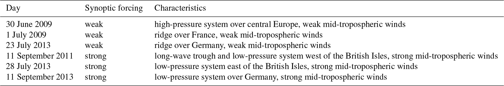
To investigate different weather regimes, we perform numerical simulations for three cases with weak synoptic forcing and for three cases with strong synoptic forcing. These are the same days already investigated by Schneider et al. (2018), who provided a detailed synoptic analysis and comparison of radar-derived and simulated precipitation totals. They showed that the model captures the overall precipitation distribution reasonably well. Thus, we only list the days and main weather characteristics in Table 2 and refer to their study for more details.
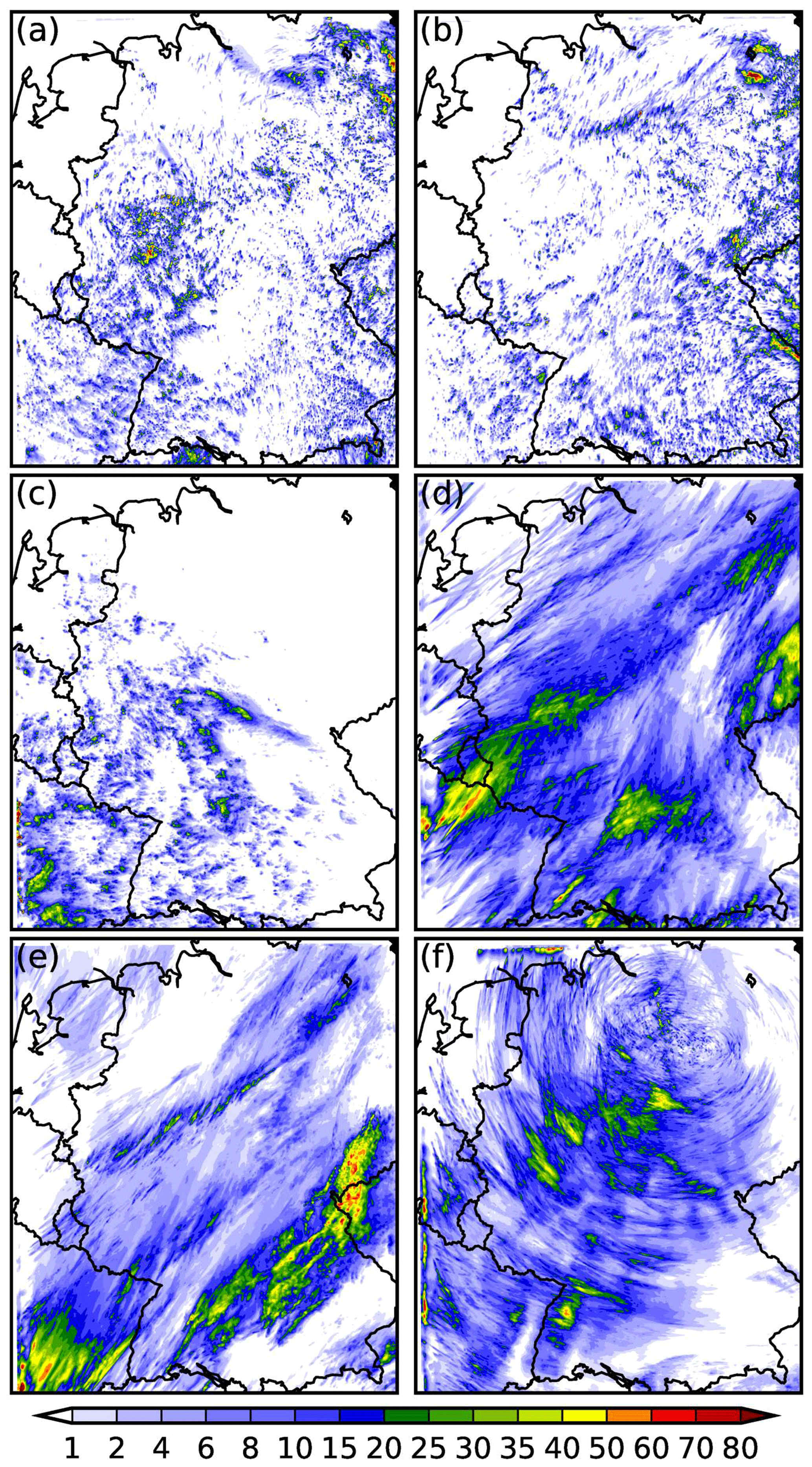
Figure 324 h precipitation amount of the 500 m grid-length reference run in millimeters for the 6 days of investigation: (a) 30 June 2009; (b) 1 July 2009; (c) 23 July 2013; (d) 11 September 2011; (e) 28 July 2013; (f) 11 September 2013. Figure adapted from Fig. 5 in Schneider et al. (2018).
The 24 h accumulated precipitation of all reference runs (500 m original orography, unchanged initial soil moisture, continental CCN assumption) is shown in Fig. 3. During weak synoptic forcing, the model simulates isolated convective cells with a lifetime of around 1–3 h (Fig. 3a–c). A more stratiform precipitation distribution is simulated for strong synoptic forcing. For these days, embedded convection (Fig. 3d, e) and orographic precipitation enhancement (Fig. 3f, southwestern Germany) are also simulated.
3.1 Precipitation amounts and timing
The precipitation response to land surface and aerosol heterogeneities is summarized using domain-averaged precipitation totals and their deviations from the respective reference run (Fig. 4). It can be seen that the average precipitation is much smaller on weak forcing days (1.6–2.8 mm) than on strong forcing days (6.0–8.1 mm). The impact of our perturbations on precipitation deviations, however, is on average higher for weak than for strong synoptic forcing. Soil moisture and aerosols are each responsible for the maximum precipitation response for three of the cases, while the sensitivity to terrain forcing always shows the smallest spread. In general, perturbations of the orography have a larger impact during weak forcing conditions, whereas for strong synoptic forcing, the impact is rather small. This could be explained by the fact that for orographic, more stratiform precipitation, the resolution of the external data is not that important, as mesoscale rising of air on mountains can still be reasonably well simulated without detailed valley structures. Interestingly, the simulations with smoothed terrain show a systematic positive offset compared to the reference run on 4 out of 6 days. Reasons for this could be the changes in near-surface temperatures, which then modify the atmospheric stability. This will be discussed in more detail in the next section.
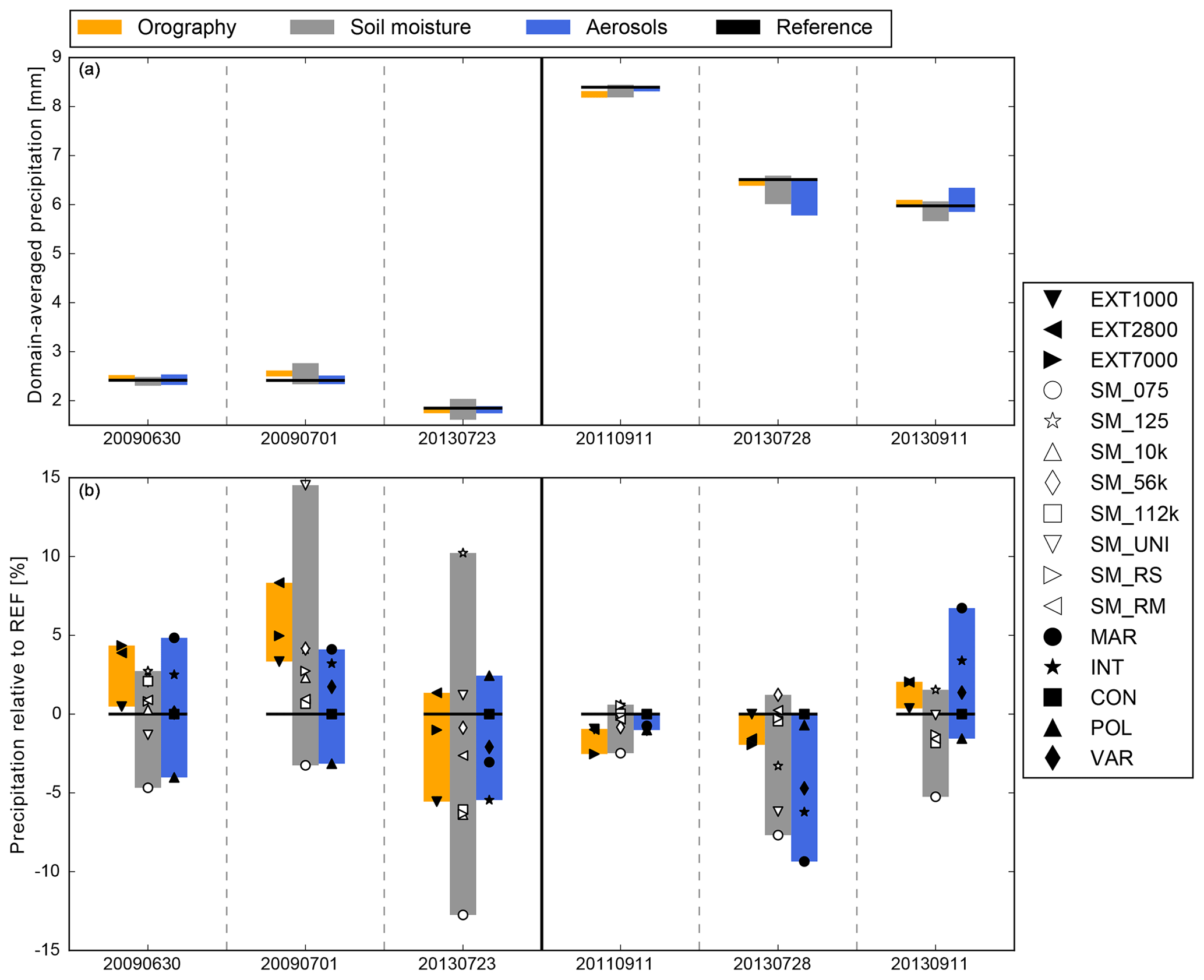
Figure 424 h domain-averaged precipitation (a) and deviation from the respective reference run (b) for the 6 days of investigation. The symbols denote the precipitation deviation and the height of the bar shows the distance between minimum and maximum mean precipitation for each set of sensitivities.
With precipitation deviations from the respective reference run between −12 % on 23 July 2013 and up to +15 % on 1 July 2009, the soil moisture simulations show the highest daily variability for weak forcing cases (Fig. 4b). Furthermore, for all analyzed cases, the runs with reduced soil moisture (SM_075) always have the lowest precipitation amounts in this group of sensitivity. Positive precipitation deviations from the reference run are simulated with increased soil moisture (SM_125), indicating a positive soil moisture–precipitation feedback (except the strong forcing case on 28 July 2013). The impact of soil moisture on precipitation totals is generally smaller for strong than for weak synoptic forcing, which implies that land surface–atmosphere interactions are less important for weather regimes with approaching troughs or frontal systems. Different patches of dry and wet soils have, on average, smaller effects on the simulated precipitation amounts than the dry or wet bias experiments. We therefore conclude that the initial soil moisture amount is much more important than the spatial distribution of dry and wet patches assuming a constant spatial average.
The response of total precipitation to changes in the CCN concentration is more complex: in three cases (30 June 2009, 1 July 2009, 11 September 2013), the precipitation amounts decrease systematically with increasing CCN. On 11 September 2011, the impact of different CCN concentrations is negligible. The remaining 2 days show a tendency towards more precipitation with higher CCN concentrations. This demonstrates the large uncertainties arising from the nonlinear character of the microphysics and the dependence of aerosol–cloud interactions on environmental conditions and cloud types. An important finding is the fact that a heterogeneous CCN distribution (VAR) with a mean concentration corresponding to that of the reference run (CON) can yield to precipitation deviations ranging in the same order of magnitude than changing the total CCN concentration.
Besides the integrated rain amounts, the timing of precipitation is also an important parameter for quantitative precipitation forecasting. From the precipitation rates given in Fig. 5, we see that the timing of precipitation is, at least for the domain average, not sensitive to the perturbations examined in this study. The days with weak synoptic forcing exhibit a typical summertime diurnal cycle with convection initiation around noon and the largest rain rates in the afternoon. Some weaker showers exist also in the early morning hours, most probably related to model spin-up effects. In contrast, strong forcing days also show significant precipitation amounts during nighttime. Based on the time evolution, we conclude that the different rain amounts of our sensitivity runs are mainly due to differences in rain intensity assuming that the number of simulated cells or their sizes do not differ substantially. The largest spread in precipitation rate agrees well with the largest deviations of the accumulated precipitation in Fig. 4.
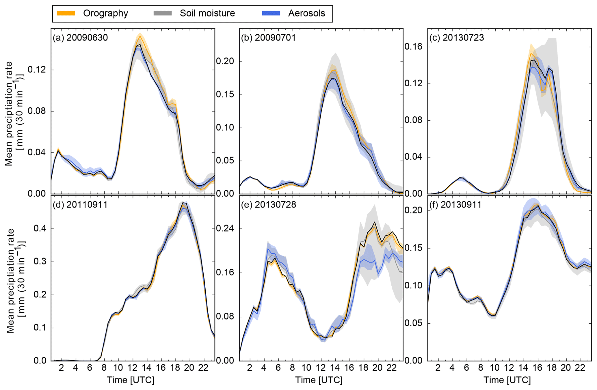
Figure 5Domain-averaged precipitation rates for the 6 days of investigation. The color-coded areas represent the spread, i.e., the maximum and minimum mean precipitation for each set of sensitivities.
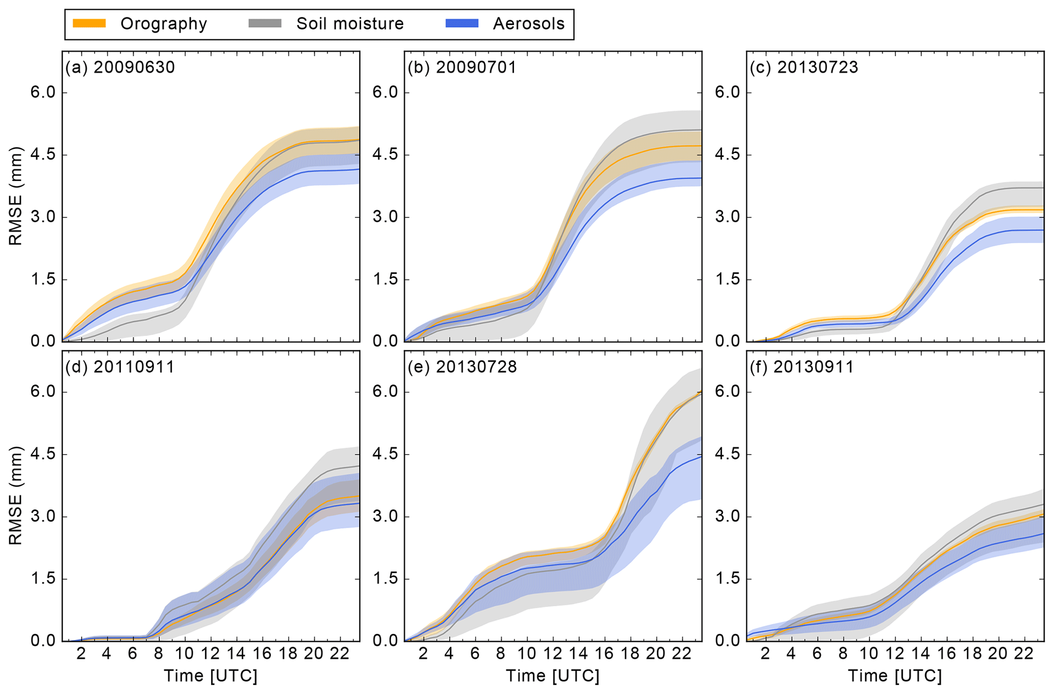
Figure 6Root mean square error (RMSE) for precipitation of the sensitivity runs compared to the reference run. Thick lines indicate the mean and color-coded areas the range between the minimum and maximum RMSE.
To further address deviations of the sensitivity runs from the reference run, we now analyze the root mean square error (RMSE) of total precipitation and its temporal evolution (Fig. 6). It can be seen that the increase in errors is generally largest for the times with maximum precipitation rates. For the weak forcing cases (Fig. 6a–c), orography and aerosol modifications lead to larger RMSE values already for smaller rain rates in the early morning hours than the soil moisture runs. Interestingly, the soil moisture runs show a steeper increase once convection is initiated around 10:00–11:00 UTC. In agreement with recent findings of Baur et al. (2018), this indicates that heterogeneous soil moisture perturbations mainly influence the convection initiation via secondary dynamical effects (like thermally induced circulations), whereas CCN and orography variations induce variability already from the beginning of the simulation. Overall, the errors are largest in the soil moisture and orography runs and smallest in the aerosol runs. This is also true for the cases with strong synoptic forcing (Fig. 6d–f). However, there is no distinct temporal delay of the soil moisture runs, indicating that its influence on precipitation initiation is weaker than on days with weak synoptic forcing. We also find that the spread at the end of the simulation of the aerosol runs is always higher for strong than for weak synoptic forcing, which points to a larger role of CCN concentrations in this weather regime. The same holds true for the soil moisture runs, which also have the largest spreads of all sensitivities studied here. On average, the orography runs have a similar spread in both weather regimes.
3.2 Object-based rainfall characterization using the SAL technique
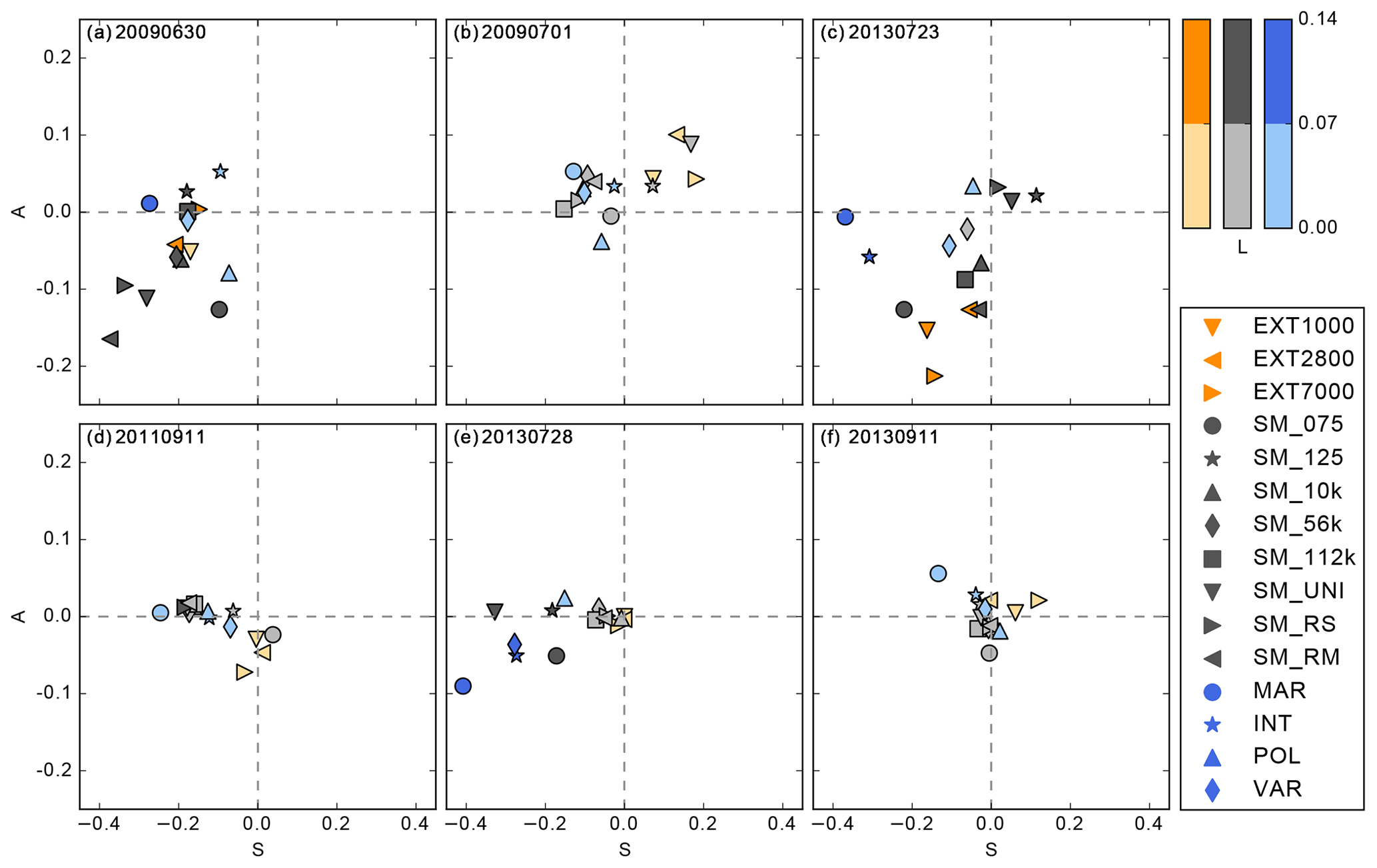
Figure 7Mean SAL diagram showing the structure, amplitude, and location component for the 6 days of investigation averaged from hourly rainfall amounts. The more the values deviate from 0, the larger the deviation from the respective reference run is. An identical prediction would have values of 0 for each component. Note the different axes for A and S.
To better quantify the precipitation characteristics in our model runs, we use the object-based structure–amplitude–location (SAL) method developed by Wernli et al. (2008). The SAL method objectively determines the characteristics of the precipitation fields by comparing the structure S, amplitude A, and location L of the simulated precipitation usually to observations for verification purposes. In this study, we apply this technique to compare the reference simulation with the rest of the sensitivity runs, similarly to the study of Henneberg et al. (2018). The amplitude component A represents the normalized differences (between −2 and +2) of the domain-averaged precipitation values and hence gives an indication whether more (A>0) or less (A<0) precipitation is simulated compared to observations or a reference simulation, thereby neglecting spatial patterns. The location component L comprises two measures: first, the normalized distance between the center of mass between the objects in the reference and sensitivity simulations, and second, the average distance between the center of mass of the individual objects and the total precipitation field. L can range between 0 and 1, and the smaller the value, the better the agreement. The structure component S compares the volume of the normalized precipitation objects by capturing their size and shape. For this, the weighted means of the normalized volume of the precipitation objects are calculated. Negative values indicate smaller or too peaked precipitation objects compared to the reference run and positive values mean the opposite. For a detailed mathematical description and examples, we refer the reader to the paper of Wernli et al. (2008). Usually, 24 h accumulated precipitation fields are compared with this technique, with the drawback that the time evolution is not considered and errors can cancel out during the day. For this reason, we compute S, A, and L values for hourly model data. These values are then averaged only for the periods with sufficient high rain intensity to avoid large SAL errors during very weak precipitation. As the S and L components both require individual precipitation objects, we apply a threshold of 1 mm h−1.
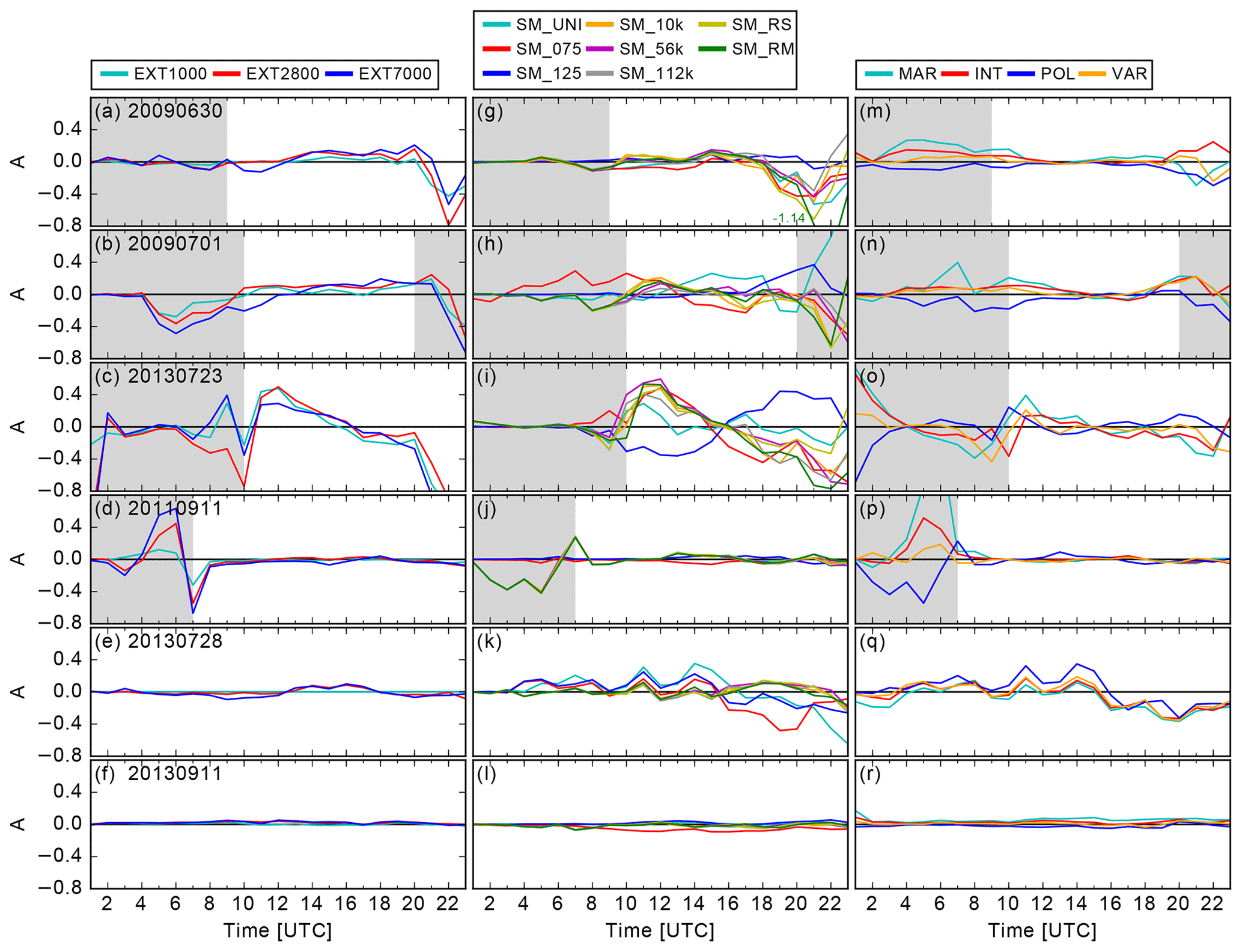
The result of this analysis is depicted in Fig. 7. The times not considered for the daily averages are marked by gray areas in Fig. 8. The mean SAL diagram shows generally smaller SAL values than in other studies (e.g., Barrett et al., 2015). This is because we compare a reference simulation to sensitivity runs and not to observations. In particular, the location component shows small values, indicating that our perturbations do not have a large impact on the location of precipitation. The days with weak synoptic forcing generally have a larger variation in their SAL components than the days with strong synoptic forcing.
The results of the SAL diagrams show most variations in the structure component (Fig. 7). Averaged for all days, the aerosol simulations have the highest absolute S value (0.15) compared to the soil moisture (0.11) or orography (0.08) simulations. The orography simulations are centered around zero S for strong synoptic forcing (Fig. 7d, e, f), which indicates that there is very little effect on the structure. This supports the previous findings, namely that changes in the terrain structure only impose a small effect on mean precipitation (Fig. 4). For the soil moisture simulations, the daily averaged S component is often negative. Whereas on weak forcing days, the individual simulations show different S values, the strong forcing cases show similar S values for the random and chessboard simulations. The aerosol simulations cover a wide range of S values for both strong and weak synoptic forcing. Very prominent is the maritime simulation, which has the most negative S component of the aerosol simulations on all days. The reason is that the maximum precipitation amounts are much higher in the maritime simulation than the other aerosol simulations. Since the structure scales with the maximum precipitation within each object, the S value is smaller in the maritime simulations than in the other aerosol simulations. The missing convection invigoration in our model, reflected by the higher rain intensities and stronger updrafts in clean conditions, was also reported by Barthlott and Hoose (2018), who stated that the model results could also be influenced by the saturation adjustment scheme to treat condensational growth. Such a scheme has been shown to enhance condensation and latent heating at lower levels, which could limit the potential for a CCN increase to increase buoyancy at mid to upper levels (Lebo et al., 2012).
The amplitude component is much smaller than the structure component, but does explain the precipitation totals well for all strong forcing days: they show an increase in precipitation compared to the reference simulation at positive A values and a decrease for negative A values (Fig. 7d, e, f). On the weak forcing days, there are simulations in which the amplitude does not reflect the precipitation sum. On 30 June 2009 (Fig. 7a), the EXT2800 and EXT7000 simulations have negative A components, while the precipitation is enhanced compared to the reference. On 1 July 2009 (Fig. 7b) the EXT7000 and on 23 July 2013 (Fig. 7c) the EXT2800 simulations do not represent the precipitation totals well. Similarly, the soil moisture simulations show good agreement of the A component with the precipitation totals under strong synoptic forcing. On 23 July 2013, the bias simulations show smaller absolute A values compared to the other soil moisture simulations, and on 30 June 2009, the random simulations show a negative A component, while they have increased precipitation amounts compared to the reference simulation. The A component of the aerosol simulations represents the mean precipitation for weak forcing cases well, except on 30 June 2009 in the INT simulations. On strong forcing days, differences exist for example on 28 July 2013, when the A component is positive in the POL run but precipitation is reduced compared to the reference simulation. Considering all days, the absolute A component for the orography is 0.05 and slightly higher than that of soil moisture and orography (0.03).
The location component is generally small (Fig. 7), meaning that the place where precipitation falls is not affected much by the uncertainties addressed in our study. For the orography simulations, the shift is somewhat higher only on 30 June 2009 (Fig. 7a) and 23 July 2013 (Fig. 7c), possibly because there is a stronger surface–atmosphere coupling during weak large-scale forcing. This would be in agreement with findings from the soil moisture simulations, as they also show higher L values for some of these days' simulations. On 28 July 2013, the bias and uniform simulation have the highest change in the location (Fig. 7e). Interestingly, the chess and random simulations show small L values, despite the formation of convergence zones due to horizontal soil moisture gradients (not shown), which could affect the location. This indicates that other mechanisms are also important for triggering convection on these days. The aerosol simulations mostly alter the location of precipitation on strong forcing days. Interestingly, the L value is very similar for orography, soil moisture, and aerosols (0.05) on all days. In summary, the amplitude and location are less affected than the structure. However, changes in the structure occur mainly due to changes in maximum precipitation amounts. Since the amplitude can explain some of the precipitation sums, we now analyze hourly time series of the A component.
3.3 Factors determining the rain amount
3.3.1 Orography
The daily averaged amplitude component did not explain the precipitation totals for 2 weak forcing days, but the time series allows for a more in-depth investigation. On 30 June 2009, the EXT7000 simulation has the highest amplitude between 12:00 and 20:00 UTC, the EXT2800 simulation is slightly smaller, and the EXT1000 simulation shows the smallest values (Fig. 8a). This result fits well to the precipitation totals. After 20:00 UTC, when the domain-averaged precipitation rate is below 0.02 mm (30 min−1), the amplitude becomes negative in all simulations, which can explain the daily mean amplitude. Similarly, on 23 July 2013, the EXT1000 simulation (Fig. 8c) has positive A values between 11:00 and 16:00 UTC. The values become very small after 20:00 UTC, which results in a negative time-averaged A value in Fig. 4.
The fact that smoothing the orography can enhance precipitation amounts despite a weaker trigger mechanism by reduced low-level wind convergence is surprising. In the following we therefore investigate why the orography simulations show more precipitation than the reference simulation on 3 days (Fig. 4) by analyzing the processes underlying these sensitivities. On 28 July 2013, the deviation is small and we will restrict the analysis to 30 June 2009, as the patterns resemble those for 1 July 2009.

Figure 9Temporal evolution of CAPE, 10 m wind convergence, and number of points with wdiff>0 m s−1 and CAPE > 600 J kg−1 on 30 June 2009 in the orography sensitivity experiments.
Before 12:00 UTC, the smoother the surface is, the weaker the low-level wind convergence (Fig. 9b). We use the velocity , which describes the difference between the simulated maximum vertical velocity (wmax) below the level of free convection and the required updraft to overcome convective inhibition (), to investigate whether convection can be initiated or not. If wdiff is positive, the updrafts are strong enough to transport air parcels to their respective level of free convection, convection will be initiated, and CAPE released (Trier, 2003). The combined measure of grid points with wdiff>0 m s−1 and CAPE > 600 J kg−1 (Fig. 9c) confirms our expectations, namely that it is more difficult to initiate deep convection with a smoother surface due to reduced low-level wind convergence. As a consequence, there is a short delay in precipitation initiation and hence CAPE has more time to build up through solar heating (Fig. 9a) only in the EXT2800 and EXT7000 simulations. Despite less favorable conditions, low-level wind convergence is still strong enough to trigger convection in these simulations. Because the static instability is higher, convection is stronger, with more precipitation than in the reference simulation. The precipitation difference between the reference and EXT1000 simulations is only minor, and so are differences in CAPE, possibly because the difference in terrain height is also marginal. We must further evaluate whether the smoothing of terrain features, leading to somewhat lower terrain heights, has any implications for the precipitable water content. The analysis of the temporal evolution of precipitable water reveals that only marginal changes with respect to the reference run occur (relative deviations ranging between −0.61 % and +0.28 %), which indicates a negligible effect.
3.3.2 Soil moisture
The A component is important to quantify the precipitation totals. However, on 30 June 2009 the daily averaged A component does not follow the precipitation totals in the simulations with random patterns. As can be seen in Fig. 8g, their values become rather small after 18:00 UTC, which mainly determines the daily average in Fig. 7. On 1 July 2009, the precipitation was reduced in the SM_075 simulation compared to the reference case, but the daily averaged amplitude was close to 0. Similarly, on 23 July 2013, the bias simulations showed a strong positive soil moisture–precipitation feedback, but the daily averaged sign in A was similar to the random simulations. We will investigate the patterns for 23 July 2013 as they are most pronounced. Interestingly, the time series of the A component shows changes in sign for all simulations (Fig. 8i). While the wet run (SM_125) shows negative values around noon, all other runs reveal positive values. Around 15:00 UTC, there is a change in sign for all model runs. Thus, the daily averaged A value is not representative. The temporal evolution of the A component fits relatively well to the temporal evolution of precipitation and can be explained by convection-related parameters (Fig. 10). The soil moisture controls the partitioning of the available energy at the surface (net radiation minus soil heat flux) into latent and sensible heat. During daytime, the Bowen ratio β (i.e., the ratio between the sensible and latent heat flux) increases to values larger than 1 in the SM_075 simulation as a result of the dominating sensible heat flux. This enhances the near-surface temperature (not shown) and turbulence in the boundary layer, which will lead to an increased low-level wind convergence compared to a simulation with enhanced soil moisture. As a result of the weaker latent heat flux, the lifting condensation level is higher (not shown) and CAPE is reduced compared to the SM_125 simulation. Despite that reduction in CAPE, the model still simulates higher rain intensities in the SM_075 simulation than in the reference run. This can be explained by the stronger lifting from low-level wind convergence and the fact that there is still enough CAPE in the atmosphere to allow for deep convection to develop. This leads to higher rain intensities between 10:00 and 14:00 UTC compared to the reference or SM_125 simulations, which are also represented by a positive A (Fig. 8i). On the other hand, CAPE can build up higher in the SM_125 simulation, and this leads to an enhancement of precipitation compared to the reference simulation after 15:00 UTC. The higher precipitation rate compared to the reference simulation is reflected in the increase in the A value (Fig. 8i) and even leads to a positive A component in the SM_125 simulation after 18:00 UTC.

Figure 10Temporal evolution of mean precipitation rate, Bowen ratio, CAPE, and 10 m wind convergence on 23 July 2013 in the soil moisture sensitivity experiments.
The random and chessboard simulations show increasing values until 12:00 UTC, remain positive until 15:00 UTC, and decrease afterwards to negative values. These mass process rates have been integrated vertically and averaged over the domain. In general, these simulations show similar values for the Bowen ratio and CAPE and only minor differences in the low-level wind convergence compared to the reference run. This leads to small differences in precipitation, which results in differences in the amplitude.
The simulations for days with strong synoptic forcing show less variations in the A component than do the days with weak forcing. On 11 September 2011 and 2013, the A component shows only small differences in all model runs. Only on 28 July 2013 do larger deviations from 0 exist for the soil moisture and aerosol uncertainties (Fig. 8k, q). The precipitation totals are in agreement with the evolution of the amplitude component on all days. As has been noted earlier, this day is the only one without a systematic soil moisture–precipitation relationship. Before 15:30 UTC, both the dry and wet simulations mostly reveal higher-amplitude components than the reference run. Later on, both time series become negative, resulting in an overall precipitation reduction compared to the reference run. In general, the surface fluxes are smaller on strong forcing days and hence the surface–atmosphere coupling is weaker. Changes that do occur mainly result from modifications in the total precipitable water as a result of small changes in evaporation (not shown).
3.3.3 Aerosols
On 30 June 2009 (Fig. 8m) between 9:00 and 19:00 UTC, on 1 July 2009 (Fig. 8n) between 9:00 and 14:00 UTC, and on 11 September 2013 (Fig. 8r), there is a tendency for decreasing amplitude from maritime to continental conditions, and so does the precipitation amount (Fig. 4). One common characteristic for these days is that the domain-averaged updraft velocities within the clouds (regions where the integrated cloud and rain water path is larger than 0.01 mg m−2) is always smaller than 0.25 m s−1 (not shown).
On 11 September 2011 there is a weak decrease in the amplitude component after 12:00 UTC from polluted to maritime conditions (Fig. 8p). On 28 July 2013, the amplitude is highest in the polluted and lowest in the maritime simulation (Fig. 8j). On 23 July 2013, the order changes at 15:00 UTC (Fig. 8o) and the precipitation sums are also less systematic. On these 3 days, the updraft velocities within clouds are always higher than 0.38 m s−1 and therefore higher than in the three cases described above. The different vertical velocities, and thus the environmental conditions, then affect the dominant cloud microphysical pathways, which are now analyzed using microphysical process rates. The warm-phase processes are autoconversion (collision of cloud droplets) and accretion (rain droplets collecting cloud droplets), and the dominant cold-phase processes are vapor deposition on ice crystals and riming (collision of a droplet and an ice crystal). In general, cold-rain processes dominate in all our simulations as the ratio of warm- to cold-rain processes is always less than 1 (Fig. 11). On 11 September 2011 and 8 July 2013, cold processes are much more important than warm processes, as indicated by the small ratio of warm- to cold-rain processes, due to the stronger lifting.
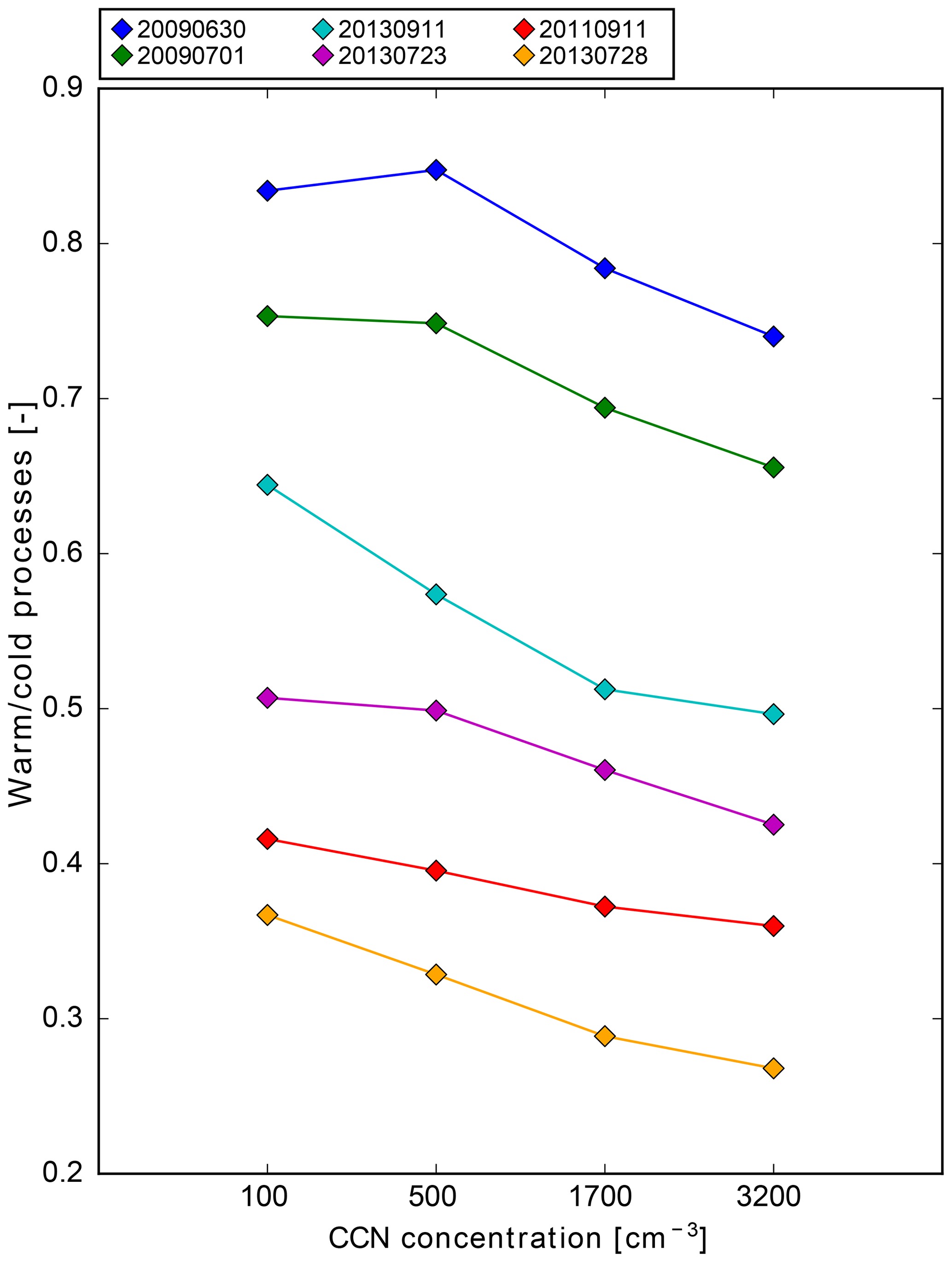
Figure 11Ratio between warm (autoconversion and accretion) and cold (vapor deposition and riming) rain processes as a function of the CCN concentration.
On 23 July 2013 the ratio is higher, possibly because we find a regime change during the high-intensity period. For these 3 days, the higher vertical velocity leads to a pronounced transport of cloud droplets towards higher altitudes, especially for polluted conditions, when cloud droplets are smaller (not shown) and hence persist longer within the clouds than is the case for maritime conditions. As mentioned earlier, we do not observe stronger updrafts in polluted conditions and thus observe no convection invigoration as hypothesized by Rosenfeld et al. (2008). Instead, when the cloud particles grow via the cold phase and then precipitate, they have bigger sizes than the droplets in the maritime conditions (not shown) and are thus less susceptible to evaporation below cloud base, which leads to higher precipitation amounts with increasing CCN.
On the other hand, warm-phase processes are almost similarly important to cold-phase processes on 30 June and 1 July 2009, due to the weaker updrafts and, even on 11 September 2013, the ratio is always above 0.5. On these days, the suppression of collision–coalescence with increasing CCN has larger effects on the precipitation amounts (as cold-phase processes and melting contribute relatively less) and hence a reduction in precipitation towards more polluted conditions. For a more detailed analysis of hydrometeor profiles and microphysical process rates, we refer the reader to Schneider (2018).
The purpose of this study was to investigate the relative contribution of orography, soil moisture, and aerosols to the predictability of deep convection. To this end, we performed 500 m grid-length numerical simulations with the COSMO model for six real-case events over Germany classified into weak and strong large-scale forcing. The sensitivities comprise smoothing the terrain, systematic changes in the initial soil moisture field, and different homogeneous and spatially heterogeneous CCN concentrations.
In general, weak forcing days show smaller precipitation amounts than strong forcing days, but a higher precipitation susceptibility (−12 to +15 %) to the applied changes than strong forcing days (−9 to +7 %). We find that uncertainties in soil moisture and CCN concentrations contribute the most to the spread in our sensitivity runs. The modifications in soil moisture have the strongest impact on 2 weak forcing days and 1 strong forcing day. For the majority of the analyzed cases, the model produces a positive soil moisture–precipitation feedback in agreement with, e.g., Findell and Eltahir (2003) or Cioni and Hohenegger (2017). Different patches of dry and wet soils have, on average, smaller effects on the simulated precipitation amounts than the dry or wet bias experiments. We therefore conclude that the initial soil moisture amount is more important than the spatial distribution of dry and wet patches assuming a constant spatial average. The aerosol simulations have the strongest impact on 1 weak forcing and 2 strong forcing days. Furthermore, we find that an increase in CCN concentrations can either lead to an increase or decrease in precipitation, depending on the environmental conditions and different contributions of warm- and cold-rain processes. In all our simulations, the contribution of cold-rain processes is higher than that of warm-rain processes. For weak updrafts, however, the relative role of the warm-phase processes is higher and a reduction in precipitation occurs with higher CCN concentrations and smaller droplets. For stronger updrafts, the cold-phase processes dominate. The precipitation thus increases with increasing CCN, as bigger raindrops that occur via the cold phase are less susceptible to low-level evaporation (Tao et al., 2007; Barthlott et al., 2017). An important finding is the fact that a heterogeneous CCN distribution with a mean concentration corresponding to that of the reference run (continental assumption) can lead to precipitation deviations ranging in the same order of magnitude than changing the total CCN concentration. The fact that soil moisture and aerosol perturbations contribute in a similar magnitude to the precipitation totals suggests that aerosols are indeed important for quantitative precipitation forecasting (Miltenberger et al., 2018). The smallest deviations from the reference runs occurred when introducing orography uncertainties. Surprisingly, on 3 days, the smoothing of terrain features led to higher precipitation amounts. This could be attributed to a slightly increased instability compensating for the weaker triggering by low-level wind convergence. In addition, the resolution of external data is less important for strong synoptic forcing as mesoscale rising of air over mountain ridges can still be reasonably well simulated without fine-scale orographic features like valleys.
To investigate amplitude, location, and structure of precipitation, we compute SAL diagrams based on hourly precipitation fields. We find that the structure parameter is affected the most, followed by the amplitude and only small variations in the location. On average, the highest structure parameters occur in aerosol simulations (absolute mean 0.15). Changes in the structure occur mainly due to increased maximum precipitation amounts. The evolution of rain intensities was mostly well correlated with the amplitude component. The location component does not vary much between the three sensitivities and the absolute value lies around 0.05. Because of this resemblance, we hypothesize that this shift is due to noise resulting from different CCN assumptions and initially small perturbations to the thermodynamics/dynamics. This is in accordance with previous findings of Schneider et al. (2018), namely that the shift in precipitation in the orography simulations resembles the patterns for artificially introduced noise. As a thorough discussion of all involved processes and feedbacks for all sensitivities and cases would be exhaustive, we refer to Schneider (2018) for more details.
To increase the reliability of operational ensembles, we will probably observe a further increase in the use of ensemble methods, but this will require more effort to perturb the model (Leutbecher et al., 2017). The overall goal for these perturbations is to make them as realistic and relevant as possible. For the operational forecast, ensembles, which perturb initial conditions, boundary data and model physics, are run to account for the various uncertainties. Based on the results of this study, we suggest accounting for variations in soil moisture and aerosols, also because both are associated with a high measurement uncertainty (e.g., Van Reken et al., 2003; Hauck et al., 2011). For the soil moisture perturbations, adapted ensembles could be meaningful, i.e., by perturbing different components depending on the large-scale synoptic situation. After all, we conclude that these uncertainties should be included in a full ensemble forecasting system containing other key sources of uncertainty to estimate their relative importance for longer periods.
COSMO model output is available on request from the authors.
CB and CH developed the project idea; they designed the numerical experiments with LS, who carried them out. AIB contributed with technical implementations to write out microphysical process rates and to use horizontal heterogeneous CCN concentrations in the COSMO model code. LS conducted the analyses and all contributed to the interpretation of the results. LS wrote the first version of the paper, and CB extensively edited it with contributions from CH and AIB.
The authors declare that they have no conflict of interest.
The authors wish to thank the Deutscher Wetterdienst (DWD) for providing the COSMO model code and the initial and boundary data. This work was performed on the computational resource ForHLR I and II funded by the Ministry of Science, Research and the Arts Baden-Württemberg and DFG (“Deutsche Forschungsgemeinschaft”). Furthermore, we wish to thank Hassan Beydoun (KIT) for fruitful discussions.
The research leading to these results has been done within the subprojects “B3: Relative impact of surface and aerosol heterogeneities on the initiation of deep convection” and “B1” of the Transregional Collaborative Research Center SFB/TRR 165 “Waves to Weather” (http://www.wavestoweather.de, last access: 2 October 2019) funded by the German Research Foundation (DFG).
The article processing charges for this open-access publication were covered by a Research Centre of the Helmholtz Association.
This paper was edited by Yves Balkanski and reviewed by two anonymous referees.
Altaratz, O., Koren, I., Remer, L., and Hirsch, E.: Review: Cloud invigoration by aerosols: Coupling between microphysics and dynamics, Atmos. Res., 140–141, 38–60, 2014. a
Baldauf, M., Seifert, A., Förstner, J., Majewski, D., and Raschendorfer, M.: Operational convective-scale numerical weather prediction with the COSMO model: description and sensitivities, Mon. Weather Rev., 139, 3887–3905, https://doi.org/10.1175/MWR-D-10-05013.1, 2011. a, b
Barrett, A. I., Gray, S. L., Kirshbaum, D. J., Roberts, N. M., Schultz, D. M., and Fairman, J. G.: Synoptic versus orographic control on stationary convective banding, Q. J. Roy. Meteorol. Soc., 141, 1101–1113, https://doi.org/10.1002/qj.2409, 2015. a
Barthlott, C. and Hoose, C.: Spatial and temporal variability of clouds and precipitation over Germany: multiscale simulations across the “gray zone”, Atmos. Chem. Phys., 15, 12361–12384, https://doi.org/10.5194/acp-15-12361-2015, 2015. a
Barthlott, C. and Hoose, C.: Aerosol effects on clouds and precipitation over central Europe in different weather regimes, J. Atmos. Sci., 75, 4247–4264, https://doi.org/10.1175/JAS-D-18-0110.1, 2018. a, b
Barthlott, C. and Kalthoff, N.: A Numerical Sensitivity Study on the Impact of Soil Moisture on Convection-related Parameters and Convective Precipitation over Complex Terrain, J. Atmos. Sci., 68, 2971–2987, https://doi.org/10.1175/JAS-D-11-027.1, 2011. a
Barthlott, C., Adler, B., Kalthoff, N., Handwerker, J., Kohler, M., and Wieser, A.: The role of Corsica in initiating nocturnal offshore convection, Q. J. Roy. Meteorol. Soc., 142, 222–237, https://doi.org/10.1002/qj.2415, 2016. a
Barthlott, C., Mühr, B., and Hoose, C.: Sensitivity of the 2014 Pentecost storms over Germany to different model grids and microphysics schemes, Q. J. Roy. Meteorol. Soc., 143, 1485–1503, https://doi.org/10.1002/qj.3019, 2017. a, b
Baur, F., Keil, C., and Craig, G.: Soil Moisture – Precipitation Coupling over Central Europe: Interactions between surface anomalies at different scales and its dynamical implication, Q. J. Roy. Meteorol. Soc., 144, 2863–2875, https://doi.org/10.1002/qj.3415, 2018. a, b
Berner, J., Achatz, U., Batté, L., Bengtsson, L., Cámara, A. d. l., Christensen, H. M., Colangeli, M., Coleman, D. R. B., Crommelin, D., Dolaptchiev, S. I., Franzke, C. L. E., Friederichs, P., Imkeller, P., Järvinen, H., Juricke, S., Kitsios, V., Lott, F., Lucarini, V., Mahajan, S., Palmer, T. N., Penland, C., Sakradzija, M., von Storch, J.-S., Weisheimer, A., Weniger, M., Williams, P. D., and Yano, J.-I.: Stochastic Parameterization: Toward a New View of Weather and Climate Models, B. Am. Meteor. Soc., 98, 565–588, https://doi.org/10.1175/BAMS-D-15-00268.1, 2017. a
Bouttier, F. and Raynaud, L.: Clustering and selection of boundary conditions for limited area ensemble prediction, Q. J. Roy. Meteorol. Soc., 144, 2381–2391, https://doi.org/10.1002/qj.3304, 2018. a
Cioni, G. and Hohenegger, C.: Effect of Soil Moisture on Diurnal Convection and Precipitation in Large-Eddy Simulations, J. Hydrometeor., 18, 1885–1903, 2017. a
Clark, P., Roberts, N., Lean, H., Ballard, S. P., and Charlton-Perez, C.: Convection-permitting models: a step-change in rainfall forecasting, Meteorol. Appl., 23, 165–181, 2016. a, b
Courault, D., Drobinski, P., Brunet, Y., Lacarre, P., and Talbot, C.: Impact of surface heterogeneity on a buoyancy-driven convective boundary layer in light winds, Bound.-Lay. Meteorol., 124, 383–403, https://doi.org/10.1007/s10546-007-9172-y, 2007. a
Doms, G., Förstner, J., Heise, E., Herzog, H.-J., Mironov, D., Raschendorfer, M., Reinhardt, T., Ritter, B., Schrodin, R., Schulz, J.-P., and Vogel, G.: A description of the nonhydrostatic regional COSMO model, Part II: Physical Parameterization, available at: http://www.cosmo-model.org (last access: 2 October 2019), 2011. a, b
Findell, K. L. and Eltahir, E. A. B.: Atmospheric controls on soil moisture-boundary layer interactions, Part I: Framework development, J. Hydrometeor., 4, 552–569, 2003. a, b
Froidevaux, P., Schlemmer, L., Schmidli, J., Langhans, W., and Schär, C.: Influence of the Background Wind on the Local Soil Moisture–Precipitation Feedback, J. Atmos. Sci., 71, 782–799, https://doi.org/10.1175/JAS-D-13-0180.1, 2014. a
Groenemeijer, P., Barthlott, C., Behrendt, A., Corsmeier, U., Handwerker, J., Kohler, M., Kottmeier, C., Mahlke, H., Pal, S., Radlach, M., Trentmann, J., Wieser, A., and Wulfmeyer, V.: Observations of kinematics and thermodynamic structure surrounding a convective storm cluster over a low mountain range, Mon. Weather Rev., 137, 585–602, https://doi.org/10.1175/2008MWR2562.1, 2009. a
Guillod, B. P., Orlowsky, B., Miralles, D., Teuling, A. J., Blanken, P. D., Buchmann, N., Ciais, P., Ek, M., Findell, K. L., Gentine, P., Lintner, B. R., Scott, R. L., Van den Hurk, B., and Seneviratne, I. S.: Land-surface controls on afternoon precipitation diagnosed from observational data: uncertainties and confounding factors, Atmos. Chem. Phys., 14, 8343–8367, https://doi.org/10.5194/acp-14-8343-2014, 2014. a
Hande, L. B., Engler, C., Hoose, C., and Tegen, I.: Parameterizing cloud condensation nuclei concentrations during HOPE, Atmos. Chem. Phys., 16, 12059–12079, https://doi.org/10.5194/acp-16-12059-2016, 2016. a, b
Hauck, C., Barthlott, C., Krauss, L., and Kalthoff, N.: Soil moisture variability and its influence on convective precipitation over complex terrain, Q. J. Roy. Meteorol. Soc., 137, 42–56, https://doi.org/10.1002/qj.766, 2011. a, b, c
Henneberg, O., Ament, F., and Grützun, V.: Assessing the uncertainty of soil moisture impacts on convective precipitation using a new ensemble approach, Atmos. Chem. Phys., 18, 6413–6425, https://doi.org/10.5194/acp-18-6413-2018, 2018. a
Hohenegger, C., Brockhaus, P., Bretherton, C. S., and Schär, C.: The Soil Moisture-Precipitation Feedback in Simulations with Explicit and Parameterized Convection, J. Climate, 22, 5003–5020, 2009. a
Imamovic, A., Schlemmer, L., and Schär, C.: Collective Impacts of Orography and Soil Moisture on the Soil Moisture-Precipitation Feedback, Geophys. Res. Lett., 44, 11682–11691, https://doi.org/10.1002/2017GL075657, 2017. a
Khain, A. P., BenMoshe, N., and Pokrovsky, A.: Factors Determining the Impact of Aerosols on Surface Precipitation from Clouds: An Attempt at Classification, J. Atmos. Sci., 65, 1721–1748, https://doi.org/10.1175/2007JAS2515.1, 2008. a
Kirshbaum, D. J., Adler, B., Kalthoff, N., Barthlott, C., and Serafin, S.: Moist Orographic Convection: Physical Mechanisms and Links to Surface-Exchange Processes, Atmosphere, 9, 80, https://doi.org/10.3390/atmos9030080, 2018. a
Kühnlein, C., Keil, C., Craig, G. C., and Gebhardt, C.: The impact of downscaled initial condition perturbations on convective-scale ensemble forecasts of precipitation, Q. J. Roy. Meteorol. Soc., 140, 1552–1562, 2014. a
Lebo, Z. J., Morrison, H., and Seinfeld, J. H.: Are simulated aerosol-induced effects on deep convective clouds strongly dependent on saturation adjustment?, Atmos. Chem. Phys., 12, 9941–9964, https://doi.org/10.5194/acp-12-9941-2012, 2012. a
Leutbecher, M., Lock, S.-J., Ollinaho, P., Lang, S. T. K., Balsamo, G., Bechtold, P., Bonavita, M., Christensen, H. M., Diamantakis, M., Dutra, E., English, S., Fisher, M., Forbes, R. M., Goddard, J., Thomas, H., J., H. R., Stephan, J., Heather, L., Dave, M., Linus, M., Sylvie, M., Sebastien, M., Sandu, I., Smolarkiewicz, P. K., Subramanian, A., Vitart, F., Wedi, N., and Weisheimer, A.: Stochastic representations of model uncertainties at ECMWF: state of the art and future vision, Q. J. Roy. Meteorol. Soc., 143, 2315–2339, https://doi.org/10.1002/qj.3094, 2017. a
Mellor, G. L. and Yamada, T.: A hierarchy of turbulence closure models for planetary boundary layers, J. Atmos. Sci., 31, 1791–1806, 1974. a
Miltenberger, A. K., Field, P. R., Hill, A. A., Shipway, B. J., and Wilkinson, J. M.: Aerosol–cloud interactions in mixed-phase convective clouds – Part 2: Meteorological ensemble, Atmos. Chem. Phys., 18, 10593–10613, https://doi.org/10.5194/acp-18-10593-2018, 2018. a
Mittermaier, M. P.: A Strategy for Verifying Near-Convection-Resolving Model Forecasts at Observing Sites, Weather Forecast., 29, 185–204, 2014. a
Noppel, H., Blahak, U., Seifert, A., and Beheng, K. D.: Simulations of a hailstorm and the impact of CCN using an advanced two-moment cloud microphysical scheme, Atmos. Res., 96, 286–301, https://doi.org/10.1016/j.atmosres.2009.09.008, 2010. a
Pan, Z., Takle, E., Segal, M., and Turner, R.: Influences of model parameterization schemes on the response of rainfall to soil moisture in the central United States, Mon. Weather Rev., 124, 1786–1802, 1996. a
Phillips, V. T. J., DeMott, P. J., and Andronache, C.: An empirical parameterization of heterogeneous ice nucleation for multiple chemical species of aerosol, J. Atmos. Sci., 65, 2757–2783, 2008. a
Picard, L. and Mass, C.: The Sensitivity of Orographic Precipitation to Flow Direction: An Idealized Modeling Approach, J. Hydrometeor., 18, 1673–1688, https://doi.org/10.1175/JHM-D-16-0209.1, 2017. a
Richard, E., Chaboureau, J. P., Flamant, C., Champollion, C., Hagen, M., Schmidt, K., Kiemle, C., Corsmeier, U., Barthlott, C., and Di Girolamo, P.: Forecasting summer convection over the Black Forest: a case study from the Convective and Orographically-induced Precipitation Study (COPS) experiment, Q. J. R. Meteorol. Soc., 137, 101–117, https://doi.org/10.1002/qj.710, 2011. a
Rihani, J. F., Chow, F. K., and Maxwell, R. M.: Isolating effects of terrain and soil moisture heterogeneity on the atmospheric boundary layer: Idealized simulations to diagnose land-atmosphere feedbacks, J. Adv. Model. Earth Syst., 7, 915–937, https://doi.org/10.1002/2014MS000371, 2015. a
Rosenfeld, D., Lohmann, U., Raga, G. B., O'Dowd, C. D., Kulmala, M., Fuzzi, S., Reissell, A., and Andreae, M. O.: Flood or Drought: How Do Aerosols Affect Precipitation?, Science, 321, 1309–1313, https://doi.org/10.1126/science.1160606, 2008. a, b
Rotunno, R. and Ferretti, R.: Mechanisms of intense Alpine rainfall, J. Atmos. Sci., 58, 1732–1749, 2001. a
Rotunno, R. and Houze, R. A.: Lessons on orographic precipitation from the Mesoscale Alpine Programme, Q. J. Roy. Meteorol. Soc., 133, 811–830, https://doi.org/10.1002/qj.67, 2007. a
Santanello, J. A., Dirmeyer, P. A., Ferguson, C. R., Findell, K. L., Tawfik, A. B., Berg, A., Ek, M., Gentine, P., Guillod, B. P., van Heerwaarden, C., Roundy, J., and Wulfmeyer, V.: Land-Atmosphere Interactions: The LoCo Perspective, B. Am. Meteor. Soc., 99, 1253–1272, https://doi.org/10.1175/BAMS-D-17-0001.1, 2018. a
Schär, C., Lüthi, D., Beyerle, U., and Heise, E.: The soil-precipitation feedback: A process study with a regional climate model, J. Climate, 12, 722–741, 1999. a
Schättler, U. and Blahak, U.: A description of the nonhydrostatic regional COSMO-model, Part V: Preprocessing: Initial and Boundary Data for the COSMO-Model, available at: http://www.cosmo-model.org (last access: 11 September 2019), 86 pp., 2017. a
Schättler, U., Doms, G., and Schraff, C.: A description of the nonhydrostatic regional COSMO-model, Part VII: User's Guide, available at: http://www.cosmo-model.org (last access: 11 September 2019), 175 pp., 2016. a
Schneider, L.: Relative impact of surface and aerosol heterogeneities on deep convection, Ph.D. thesis, Institute of Meteorology and Climate Research (IMK-TRO), Karlsruhe Institute of Technology (KIT), Germany, 124 pp., https://doi.org/10.5445/IR/1000088510, 2018. a, b
Schneider, L., Barthlott, C., Barrett, A. I., and Hoose, C.: The precipitation response to variable terrain forcing over low mountain ranges in different weather regimes, Q. J. Roy. Meteorol. Soc., 144, 970–989, https://doi.org/10.1002/qj.3250, 2018. a, b, c, d, e, f
Schumacher, R. S., Schultz, D. M., and Knox, J. A.: Influence of Terrain Resolution on Banded Convection in the Lee of the Rocky Mountains, Mon. Weather Rev., 143, 1399–1416, https://doi.org/10.1175/MWR-D-14-00255.1, 2015. a
Seifert, A. and Beheng, K. D.: A two-moment cloud microphysics parameterization for mixed-phase clouds, Part I: Model description, Meteorol. Atmos. Phys., 92, 45–66, 2006. a
Seifert, A., Köhler, C., and Beheng, K. D.: Aerosol-cloud-precipitation effects over Germany as simulated by a convective-scale numerical weather prediction model, Atmos. Chem. Phys., 12, 709–725, https://doi.org/10.5194/acp-12-709-2012, 2012. a
Seneviratne, S. I., Corti, T., Davin, E. L., Hirschi, M., Jaeger, E. B., Lehner, I., Orlowsky, B., and Teuling, A. J.: Investigating soil moisture-climate interactions in a changing climate: A review, Earth-Sc. Rev., 99, 125–161, https://doi.org/10.1016/j.earscirev.2010.02.004, 2010. a, b
Tao, W.-K., Li, X., Khain, A., Matsui, T., Lang, S., and Simpson, J.: Role of atmospheric aerosol concentration on deep convective precipitation: Cloud–resolving model simulations, J. Geophys. Res.-Atmos., 112, D24S18, https://doi.org/10.1029/2007JD008728, 2007. a
Taylor, C. M., de Jeu, R. A. M., Guichard, F., Harris, P. P., and Dorigo, W. A.: Afternoon rain more likely over drier soils, Nature, 489, 423–426, 2012. a
Theunert, F. and Seifert, A.: Simulation Studies of Shallow Convection with the Convection-Resolving Version of DWD Lokal-Modell, available at: http://www.cosmo-model.org (last access: 11 September 2011), 2006. a
Tiedtke, M.: A comprehensive mass flux scheme for cumulus parameterization in large-scale models, Mon. Weather Rev., 117, 1779–1800, 1989. a
Trier, S. B.: Convective storms – convective initiation, in: Encyclopedia of atmospheric sciences, Vol 2., edited by: Holton, J. R., Curry, J. A., and Pyle, J. A., Academic Press, London, 2003. a
van den Heever, S. C., Stephens, G. L., and Wood, N. B.: Aerosol indirect effects on tropical convection characteristics under conditions of radiative-convective equilibrium, J. Atmos. Sci., 68, 699–718, 2011. a
Van Reken, T. M., Rissman, T. A., Roberts, G. C., Varutbangkul, V., Jonsson, H. H., Flagan, R. C., and Seinfeld, J. H.: Toward aerosol/cloud condensation nuclei (CCN) closure during CRYSTAL–FACE, J. Geophys. Res.-Atmos., 108, 4633, https://doi.org/10.1029/2003JD003582, 2003. a
Wernli, H., Paulat, M., Hagen, M., and Frei, C.: SAL–A Novel Quality Measure for the Verification of Quantitative Precipitation Forecasts, Mon. Weather Rev., 136, 4470–4487, https://doi.org/10.1175/2008MWR2415.1, 2008. a, b
Wicker, L. J. and Skamarock, W. C.: Time-splitting methods for elastic models using forward time schemes, Mon. Weather Rev., 130, 2088–2097, 2002. a