the Creative Commons Attribution 4.0 License.
the Creative Commons Attribution 4.0 License.
 | 29 Jan 2019
Long-term simulation of the boundary layer flow over the double-ridge site during the Perdigão 2017 field campaign
Johannes Wagner
Thomas Gerz
Norman Wildmann
Kira Gramitzky
The Perdigão campaign 2017 was an international field campaign to measure the flow and its diurnal variation in the atmospheric boundary layer over complex terrain. A huge data set of meteorological observations was collected over the double-hill site by means of state-of-the-art meteorological measurement techniques. A focus of the campaign was the interaction of the boundary layer flow with a single wind turbine, which was located on the south-western (SW) ridge top. In this study, a long-term nested large-eddy simulation (LES) of 49-day duration with a maximum horizontal resolution of 200 m is used to describe both the general meteorological situation over Spain and Portugal and the local small-scale flow structures over the double hill during the intensive observation period (IOP). The simulations show that frequently observed nocturnal low-level jets (LLJs) from the NE have their origin over the slopes of the elevated plateau between the Portuguese Serra da Estrela and the Spanish Sierra de Gata mountain ranges N and NE of Perdigão and that the diurnal clockwise turning of the wind direction over the double ridge is induced by slope and valley winds under weak synoptic conditions. It is found that, in spite of the long simulation time, modelled and observed wind structures on the ridge tops agree well, while along-valley flow within the valley is underestimated by the model.
- Article
(12432 KB) - Full-text XML
- BibTeX
- EndNote


The generation of electrical power from wind turbines (WTs) is a worldwide fast-growing industry and a key technique to extend renewable energy (Emeis, 2013). Most of the areas that are available for onshore wind parks in flat terrain have already been exploited on the European continent and further wind farms need to be installed in topographically complex terrain (Schulz et al., 2014). The precondition to operate wind farms economically under these conditions is the ability to understand and simulate the planetary boundary layer (PBL) flow in complex terrain and its interaction with WTs (Tian et al., 2013). A large number of flow phenomena, such as thermally driven flows, gravity-wave-induced downslope wind storms and rotors, are common over complex terrain and difficult to simulate with numerical models. Of special interest for wind park operators is the improved forecast of low-level jets (LLJs) (Storm et al., 2009). These are a worldwide phenomenon occurring where a local wind maximum is observed close to the ground and they can develop both over large areas (e.g. the Great Plains in the US; Rife et al., 2010) and very localized over complex terrain regions (e.g. within small valleys and basins; Banta et al., 2004). LLJs are important for the formation of heavy precipitation events and for the transport of dust and aerosols over large distances (Monaghan et al., 2010). Moreover, they are a significant source for wind power generation due to increasing WT hub heights. Due to the shallow structure of the mostly nocturnal jets, the correct simulation of LLJs with operational weather models is a challenge. It requires a sufficiently high horizontal and vertical grid resolution and a realistic representation of geographic features, such as topography, land use and surface roughness in the models.
In order to provide a new data set of PBL flow over complex terrain including the interaction with a single WT, the international field campaign Perdigão 2017 was organized in the context of the New European Wind Atlas (NEWA; Mann et al., 2017) project to measure the flow over a nearly parallel double-hill topography in the Portuguese back country (Fernando et al., 2018). The double-ridge site was chosen as it allows a smooth transition from idealized to complex terrain. This simplifies the application of both idealized and realistic numerical modelling. In addition, the region around Perdigão is known for its frequent occurrence of diurnally changing NE and SW flows, which might be induced by thermally driven LLJs. The massive instrumentation during the intensive observation period (IOP) of the field campaign with i.a. up to 49 meteorological towers, 28 Doppler wind lidars and 6-hourly radiosonde launches, provided a huge data set of meteorological observations, which can be used to test and verify numerical simulations1. In this study, a long-term large-eddy simulation (LES) is used to characterize the meteorological conditions and to identify dominant flow patterns during the IOP with a focus on LLJ events. Observational data are used to verify simulation results and to reveal potential for model improvement.
The paper is organized as follows: in Sect. 2, the set-up of the numerical model is described. Dominating meteorological flow patterns during the field campaign are presented in Sect. 3 and simulation results are compared to observations in Sect. 4. Dominating LLJ mechanisms are analysed in Sect. 5, and a conclusion is given in Sect. 6.
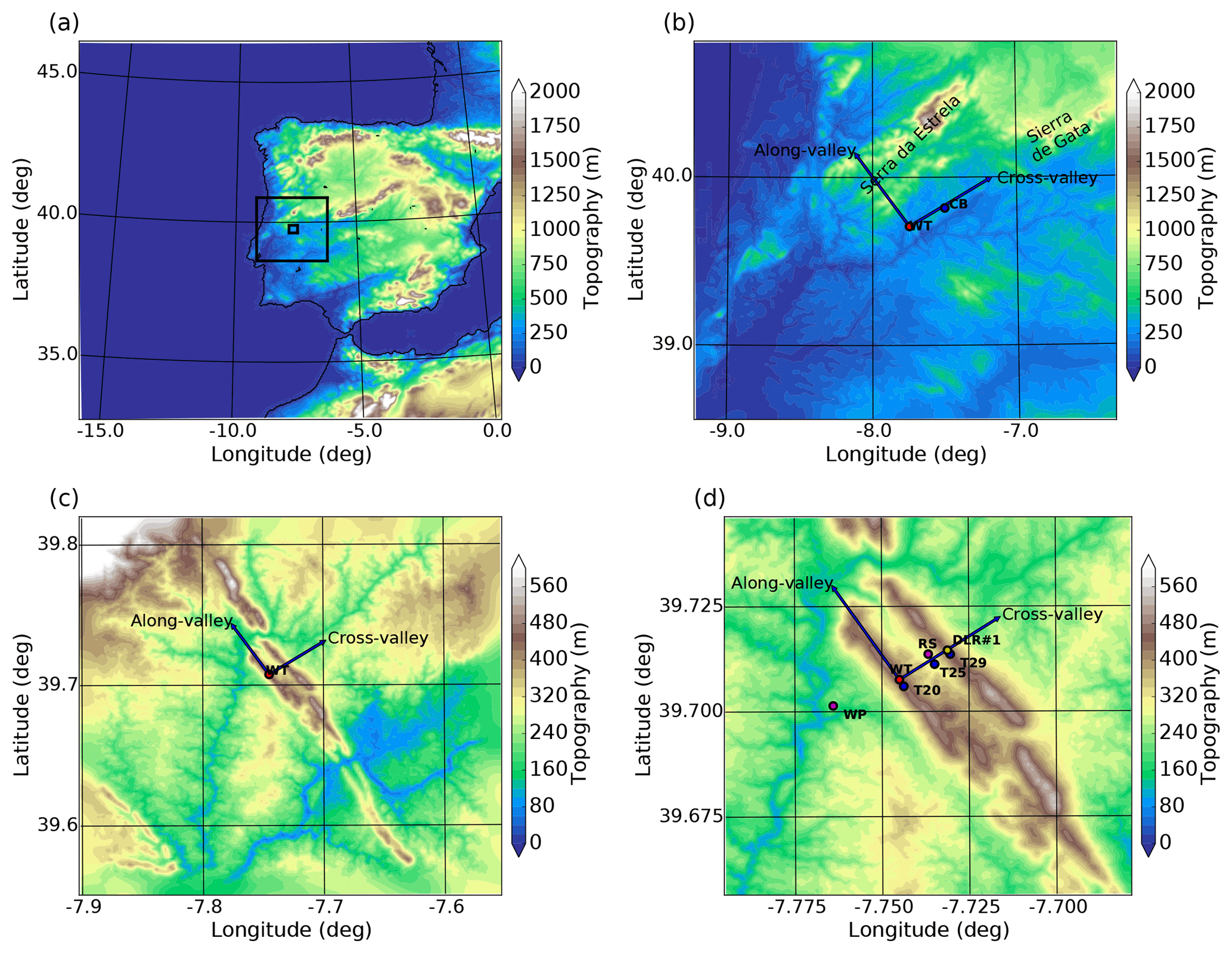
Figure 1Topographic map of Spain and Portugal and operational area of the Perdigão field campaign. The shown areas in panel (a) mark the modelling domains D1 to D3. In panels (b) and (c), the topography of domains D2 and D3 is shown. The red dot marks the position of the wind turbine (WT) on the SW ridge, and the town of Castelo Branco (CB) is marked with a blue dot in panel (b). In panel (d), the double ridge of domain D3 is enlarged to indicate the location of the WT, the three 100 m towers referred to as T20 (tower 20/tse04), T25 (tower 25/tse09) and T29 (tower 29/tse13), the Doppler wind lidar DLR no. 1, the wind profiler (WP) and the launch site of the radiosondes (RSs). The blue perpendicular arrows in panels (b) to (d) mark cross- and along-valley wind directions. Cross-valley winds are defined by the location of the WT and wind lidar DLR no. 1.
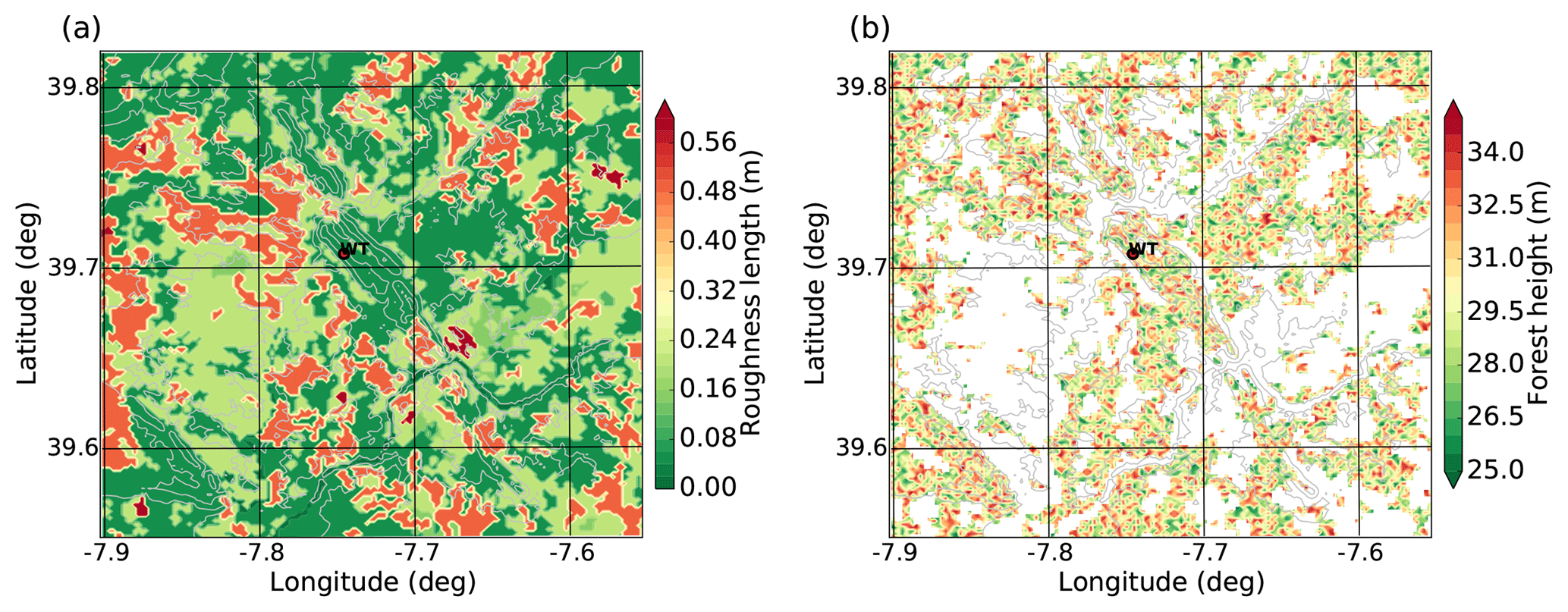
Figure 2Surface roughness length of (a) the CORINE data set and (b) tree heights of the additionally implemented forest friction term applied to domain D3. White areas are not covered by forest. The location of the WT is marked with the red dot and the topography is indicated with grey contour lines.
In this study, a long-term simulation is performed with the Weather Research and Forecasting (WRF) model version 3.8 (Skamarock et al., 2008). Three nested domains (D1, D2 and D3) with horizontal resolutions of 5 km, 1 km and 200 m are used (see Fig. 1). Domains D1 and D2 are run in RANS (Reynolds-averaged Navier–Stokes) mode, while domain D3 is run in LES mode (see below for details on differences between these two modes). A grid size of 200 m was necessary to resolve the double-ridge topography of Perdigão and its interaction with the PBL flow with at least seven grid points (the distance between the two ridges is about 1.4 km). The LES set-up was chosen to be independent of boundary layer parameterizations in domain D3, although a horizontal resolution of 200 m is relatively coarse for a LES run. Note that no mechanism was implemented in WRF to generate turbulence at the lateral edges of the LES domain, e.g. similar to the method described in Muñoz-Esparza et al. (2017). The application of such methods requires considerably higher grid resolutions of the order of 50 m for convective and 10 m for stably stratified conditions (Muñoz-Esparza et al., 2017; Muñoz-Esparza and Kosović, 2018), which is not feasible for a long-term simulation. It is therefore not the focus of this study to simulate realistic turbulence over the double ridge but to reproduce the mesoscale flow over complex terrain. Vertical nesting is applied to define individual levels in the vertical for each model domain. This helps to avoid large grid aspect ratios near the surface and to save computational resources (Daniels et al., 2016). For domains D1–D3, 36, 57 and 70 vertically stretched levels are used and the respective lowest model levels are set to 80, 50 and 15 m above ground level (a.g.l.). The model top is defined at 200 hPa (about 12 km height) to include radiation and cloud effects at the tropopause. At the model top, a 3 km thick Rayleigh damping layer (Klemp et al., 2008) is applied to prevent wave reflection. Physical parameterizations contain the Rapid Radiative Transfer Model long-wave scheme (Mlawer et al., 1997), the Dudhia short-wave scheme (Dudhia, 1989), the Yonsei University (YSU) boundary layer scheme (Hong et al., 2006), the Noah land surface model (Chen and Dudhia, 2001), the WRF single-moment five-class microphysics scheme (WSM5; Hong et al., 2004; Hong and Lim, 2006) and the Kain–Fritsch cumulus parameterization scheme (Kain and Fritsch, 1990). In domain D3, the boundary layer and cumulus schemes are switched off (LES mode) and subgrid-scale turbulence is parameterized by a three-dimensional 1.5-order turbulent kinetic energy (TKE) closure (Deardorff, 1980). The simulation is initialized once at 00:00 UTC on 30 April 2017 and run for 49 days and 18 h until 18:00 UTC on 18 June 2017. The initial and boundary conditions are supplied by European Centre for Medium-Range Weather Forecasts (ECMWF) operational analyses on 137 model levels with a horizontal resolution of 8 km and a temporal resolution of 6 h. The WRF output interval of domain D3 was set to 10 min to allow a better comparison with tower measurements averaged over 10 min.
For domains D1 and D2, the Global 30 Arc-Second Elevation (GTOPO30) digital elevation model and the US Geological Survey (USGS) land-use data set are used. These are provided by the WRF preprocessing system (WPS). For domain D3, the Advanced Spaceborne Thermal Emission and Reflection Radiometer (ASTER) topography data set (Schmugge et al., 2003) with a horizontal resolution of 30 m and the Coordination of Information on the Environment (CORINE) land cover data with a horizontal resolution of 100 m is used to better resolve the double-ridge topography and land cover of the Perdigão region. The CORINE land-use categories were transformed into the 24 USGS WRF land-use types according to Pineda et al. (2004). The inspection of surface roughness lengths from CORINE land-use data indicates that roughness lengths are considerably too small. For example, Fig. 2a shows that CORINE roughness lengths are of the order of 0.1 m over the double ridge. In reality, the hills were partially covered by eucalyptus trees with heights of about 20 to 25 m, which should be represented by roughness lengths of the order of 1 to 2 m. Short-term standard WRF simulations of LLJ cases over Perdigão were run for 12 h and showed that surface winds were clearly too high over the double-ridge region compared to lidar measurements (results will be shown in a successive paper). This was improved by the implementation of an additional friction term in LES domain D3 in the form of the forest parameterization described by Shaw and Schumann (1992), which acts on the lowermost model levels. The friction term was activated on grid points, which were classified as forest in the CORINE land-use data set (see Fig. 2b). Tree heights in these forest areas were randomly distributed by 30 m ± 5 m and were defined somewhat higher in the model compared to real tree heights (about 25 m) to ensure that at least the lowermost two to three model levels are located within the canopy layer. An overview of the described model set-up is shown in Table 1.
Table 1Overview of the WRF model set-up. Variables indicate the horizontal resolution (Δx) and the minimum distance of levels in the vertical near the surface (Δzmin). The number of grid points in x, y and z directions is marked with nx,ny and nz, respectively.
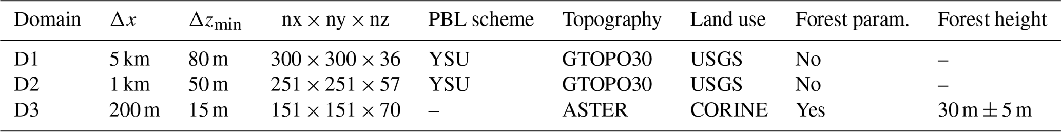
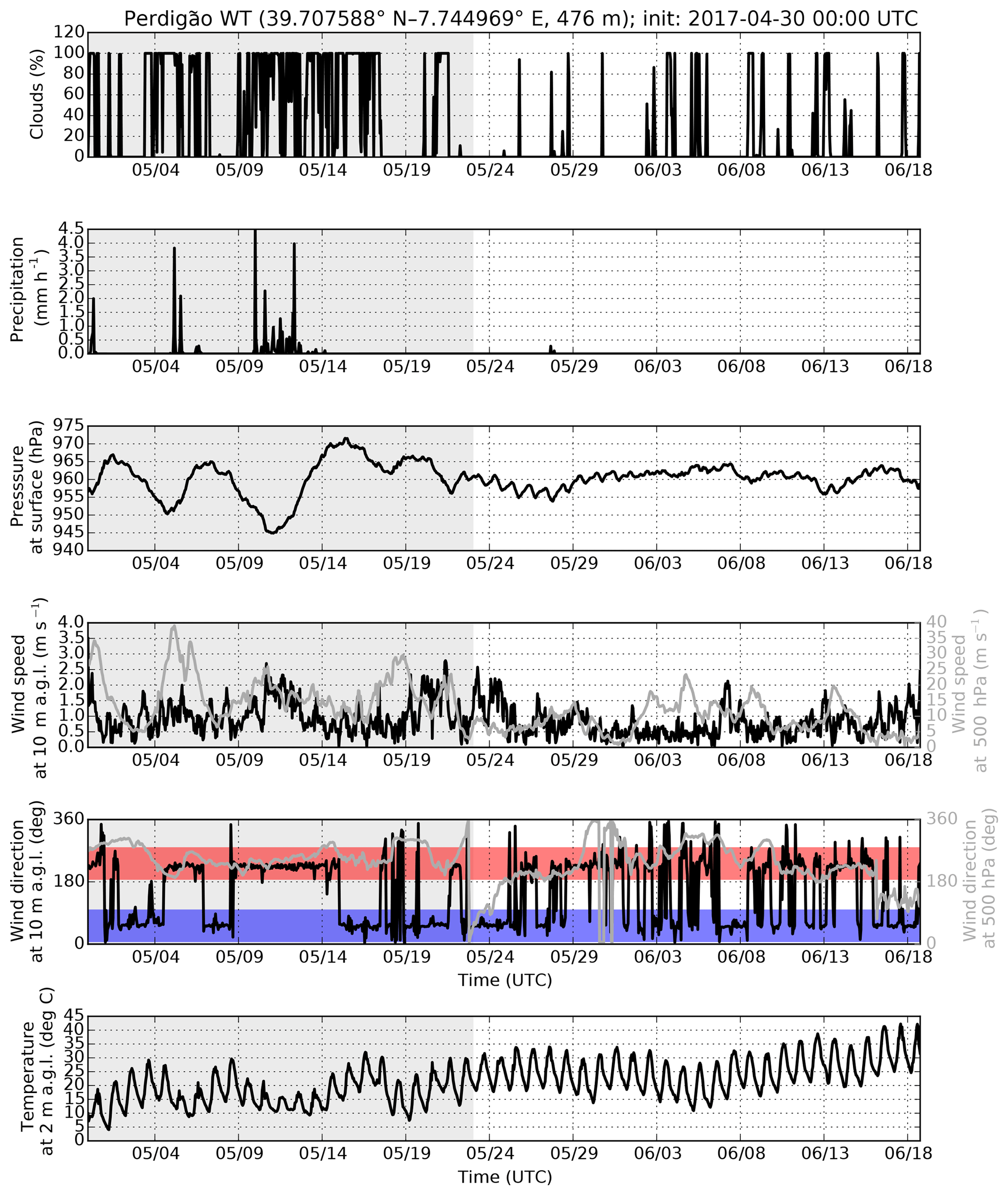
Figure 3WRF D3 meteogram for 30 April to 18 June 2017 at the location of the WT on the SW ridge. The red and blue shaded areas in the wind direction plot mark cross-valley surface winds from the SW and NE directions, respectively. The grey shading separates the campaign synoptically into phase I and phase II. Dates are in mm/dd format.
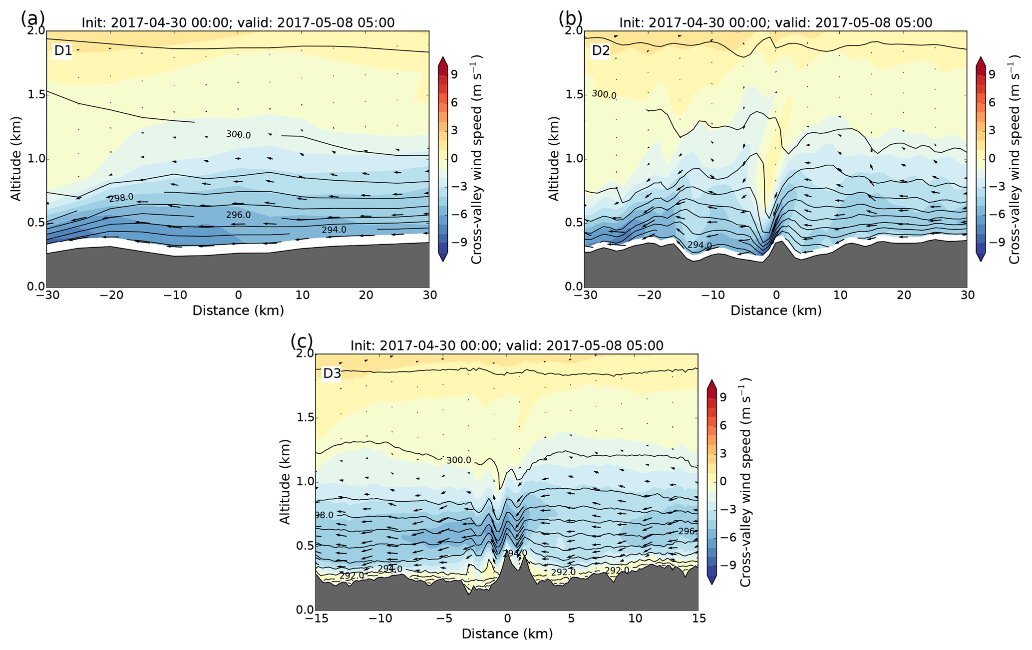
Figure 4Vertical cross-sections of cross-valley wind speed for WRF domains D1 to D3 valid at 05:00 UTC on 8 May 2017. The cross-section is centred at the location of the WT and is oriented in the cross-valley direction (see Fig. 1). In panel (c), only the half horizontal distance is shown compared to panels (a) and (b).
The IOP of the Perdigão field campaign took place from 1 May to 15 June 2017 (Fernando et al., 2018). The instrumentation was based on 49 meteorological towers (UCAR/NCAR – Earth Observing Laboratory, 2018a) with heights between 10 and 100 m, more than 180 sonic anemometers, 21 scanning and 7 profiling wind lidars (e.g. Wildmann et al., 2018b), three microwave radiometers (MWRs), a radio acoustic sounding system (RASS) wind profiler (WP; UCAR/NCAR – Earth Observing Laboratory, 2017) and 6-hourly radiosonde (RS; UCAR/NCAR – Earth Observing Laboratory, 2018b) launches. On the southwestern (SW) ridge, an Enercon E-82 2 MW WT with a hub height of 78 m and a rotor diameter of 82 m is located (see Fig. 1). Sound propagation and immission were measured by nine microphones on the up- and downstream sides of the SW ridge. In this study, data of the WP, RS observations and tower measurements of towers T20 (tower 20/tse04), T25 (tower 25/tse09) and T29 (tower 29/tse13) were used (see Fig. 1). Time series of vertical profiles of WRF data at the locations of the three 100 m towers (T20, T25, T29) are available online for all three modelling domains (DLR Institut für Physik der Atmosphäre – WRF long-run, 2019). As the main wind directions at Perdigão are NE and SW flows, the focus in this study is on flow perpendicular (cross-valley) and parallel (along-valley) to the double ridge. The direction of cross- and along-valley winds is marked with the blue arrows in Fig. 1b to d. Cross-valley winds were defined along the cross-section of the DLR no. 1 wind lidar and are therefore not perfectly perpendicular to the double ridge. Along-valley winds are defined to be perpendicular to cross-valley winds. Negative cross- and along-valley winds indicate winds from the NE and NW directions, respectively.
To give an overview of the meteorological conditions during the campaign, a WRF meteogram of domain D3 for the location of the WT is shown in Fig. 3. Based on the synoptic conditions, the campaign can be divided into two phases. During the first phase from 1 to about 23 May, the Perdigão region was influenced by periodic passages of low- and high-pressure systems, as is visible from the surface pressure time series. Low-pressure systems were accompanied by precipitation events, increased cloudiness, reduced diurnal surface temperature variation and cross-valley winds at 10 m a.g.l. from the SW (wind direction sector marked with red shading in Fig. 3). During high-pressure events, wind speed and wind direction at 500 hPa represent the conditions in the free atmosphere and show that winds were blowing from western directions throughout the first phase of the campaign. Surface winds were decoupled from the free atmosphere during the night and thermally driven LLJs from the NE developed (wind direction sector marked with blue shading in Fig. 3), e.g. in the period from 2 to 3 May, 7 to 8 May or 16 to 17 May. As an example, a typical LLJ case on 8 May 2017 at 05:00 UTC is shown in Fig. 4 by means of vertical cross-sections of cross-valley wind for WRF domains D1 to D3. Similar situations occurred frequently during the campaign. In all three domains, strong winds from the NE are visible; however, only in domain D3 is the double ridge resolved, and a LLJ including lee waves is generated. In D1 and D2, the topography is strongly smoothed and no LLJ develops due to strongly overestimated winds near the surface. In D1, the Perdigão topography is nearly flat and in D2 only one single hill exists. In both domains, no valley boundary layer including recirculation and along-valley flows can develop, which results in considerable deviations from observed winds (see the following section).
During the second phase starting on about 23 May (see Fig. 3), the subtropical tropospheric jet stream moved further north and the Iberian Peninsula was located under stable high-pressure conditions. During this phase, cloud coverage and rain events decreased significantly, while diurnal surface temperature variations and daily temperature maxima increased until the end of the campaign. In the free atmosphere, winds were weaker in comparison to the first phase and there were cases with non-western wind directions at 500 hPa (e.g. 23 May, 28 May, 12 June). Surface winds were often super-geostrophic compared to winds at the 500 hPa level and showed a more frequent diurnal variation of SW and NE winds compared to the first phase. This can be explained by the development of thermally driven wind systems, which were favoured under weak synoptic conditions and are analysed in more detail in Sect. 5.
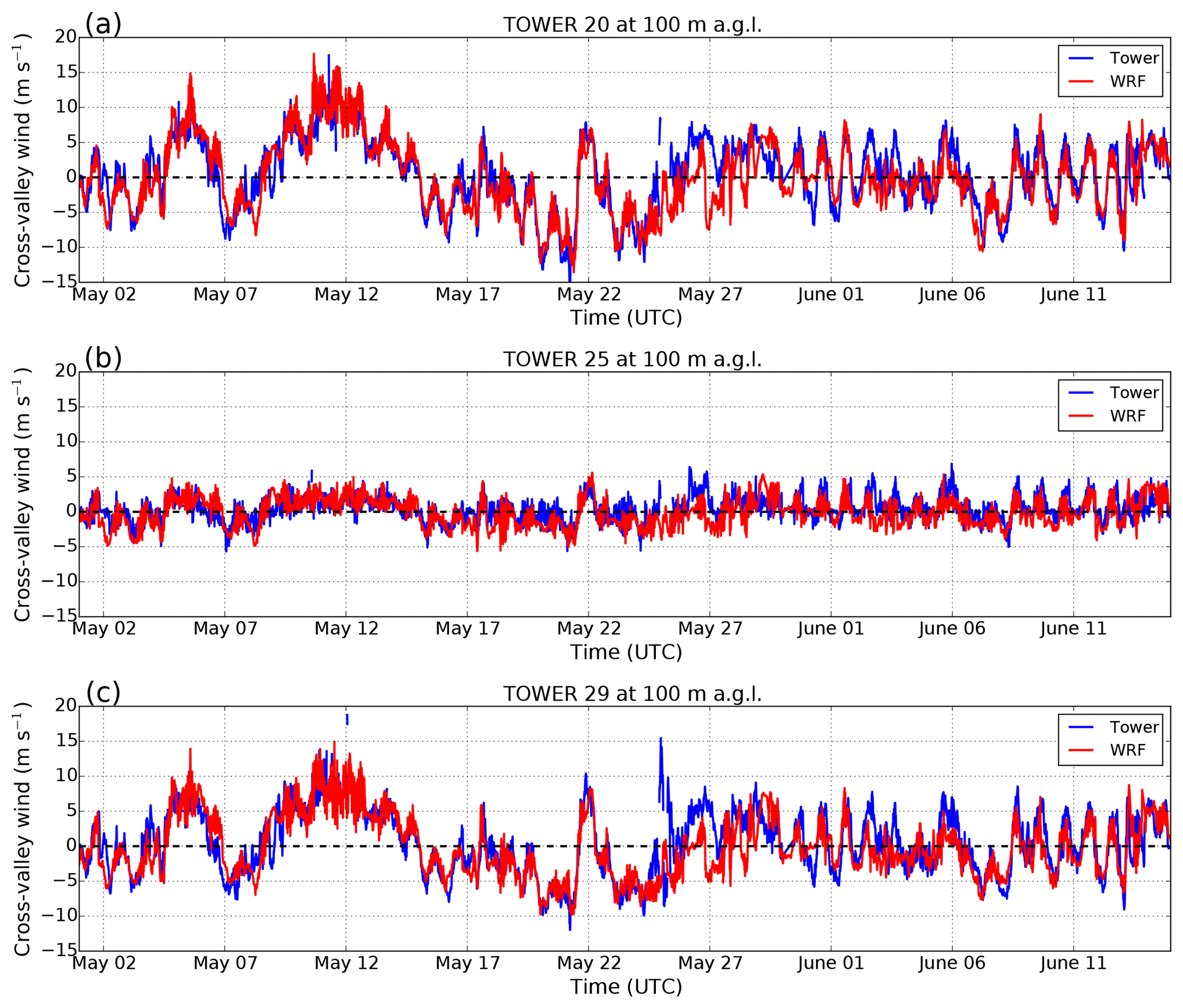
Figure 5Time series of observed and simulated (WRF D3) cross-valley wind at 100 m a.g.l. for (a–c) towers T20, T25 and T29 (see Fig. 1c for tower locations).
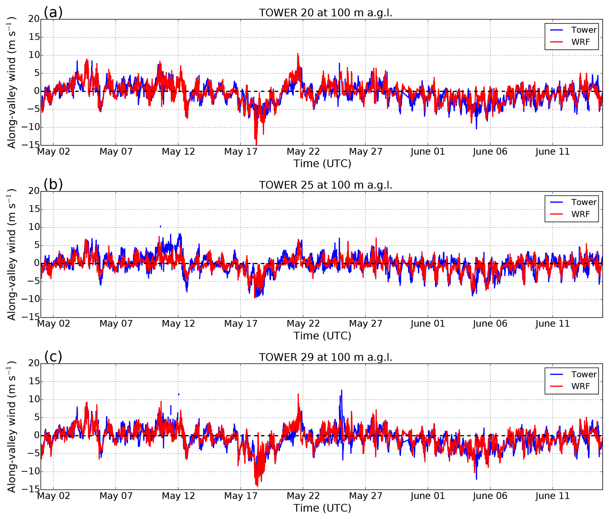
The data set of remote and in situ observations obtained during the Perdigão campaign enables to evaluate the long-term simulation. Figures 5 and 6 show observed and simulated WRF D3 time series of cross- and along-valley winds at 100 m a.g.l. at the locations of towers T20, T25 and T29 (see Fig. 1 for the tower locations). The output interval of both data sets was 10 min. Simulated cross- and along-valley winds show very good agreement with all three tower stations. Both absolute values and phase of the observed signal are reproduced well by the model. It has to be recapitulated that the model was only initialized once and was run for a period of 49 days. The lateral boundaries of domain D1, where ECMWF data serve as boundary conditions, are 750 km away from the Perdigão site (see Fig. 1a). Within the WRF domains, the model develops its own dynamics and is able to reproduce the diurnally changing flow systems during the whole simulation period with a surprisingly high quality. The comparison of towers T20 and T29 in Fig. 5a and c shows similar time series of cross-valley winds, as these towers were located on the SW and NE ridges, respectively, and probed the PBL at the same altitude. Especially during phase II, diurnally changing NE and SW flows are visible from both T20 and T29 measurements and model simulations. Due to the location within the valley, tower T25 in Fig. 5b shows much weaker cross-valley winds. Along-valley winds (Fig. 6) at T20 and T29 on the ridge tops are significantly lower than cross-valley winds on the ridge tops. In the valley at T25, along-valley winds seem to be the dominant wind component and reveal diurnal changing NW and SE flows. For both cross- and along-valley winds, correlation coefficients and root mean square errors (RMSEs) were computed for T20, T25 and T29 for WRF domains D1 to D3 (see Table 2). The highest correlations are found on the ridge tops (T20 and T29) and surprisingly the correlation coefficients are very similar for all WRF domains. This means that the phase of the (diurnally) changing cross- and along-valley wind signals can be reproduced by the two coarse model domains (D1 and D2), although they do not resolve the double ridge. This can be explained by the fact that changing NE and SW winds are thermally driven by a mesoscale horizontal pressure gradient (see next section), which is resolved by D1 and D2. The high grid resolution of domain D3 improves local effects over the double ridge but does not increase the correlation. The correlation coefficient alone is, however, not sufficient to assess the model performance. Looking at RMSE values, domain D3 reveals considerably reduced errors (up to 2.3 m s−1 at T25) compared to the coarser-resolved domains. This is due to the better representation of topographically induced flow patterns, especially within the valley (T25).
Table 2Correlation coefficient (COR) and root mean square error (RMSE) values for the comparison of WRF data with observations at towers T20, T25 and T29. Values for cross- (along-)valley winds are written in bold (normal) font.
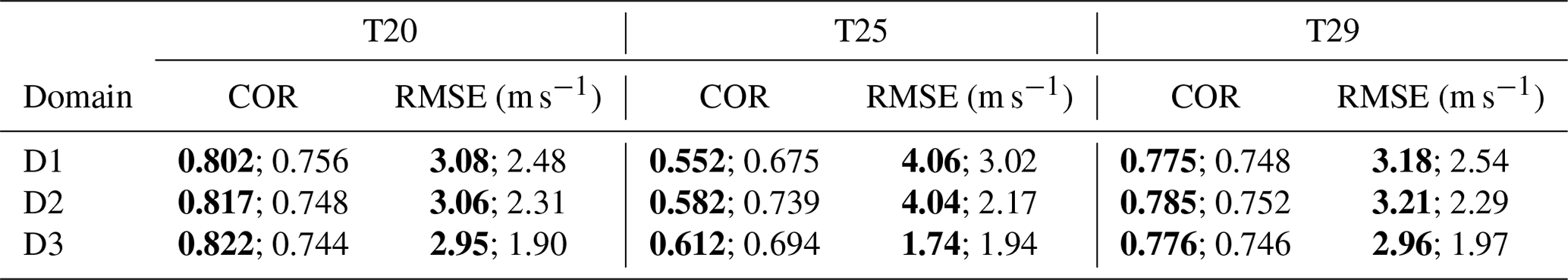
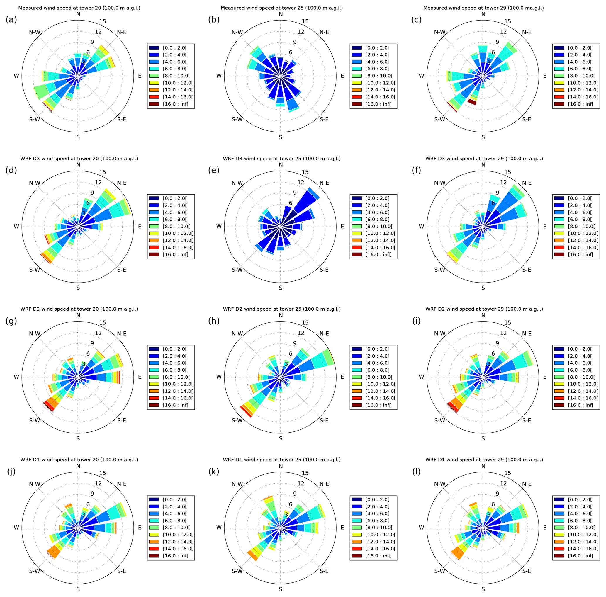
Figure 7Wind distribution at 100 m a.g.l. for observed (a–c) and simulated horizontal winds for (d–f) domain D3, (g–i) domain D2 and (j–l) domain D1. The columns from the left to the right correspond to the locations of towers T20, T25 and T29, respectively (see Fig. 1c for tower locations).
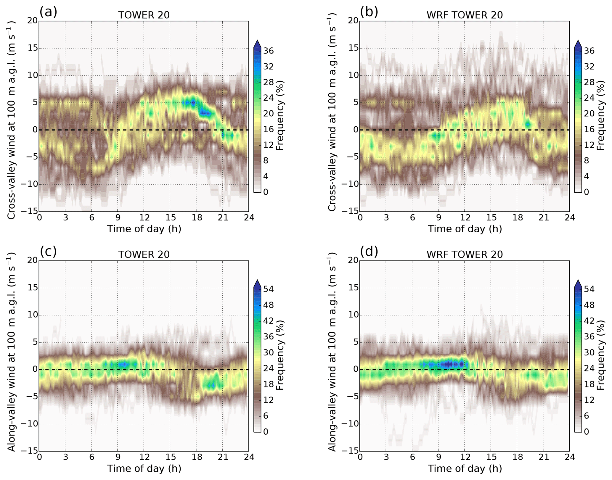
Figure 8Diurnal distribution of (a, b) cross- and (c, d) along-valley winds at 100 m a.g.l. at tower T20 in the period 1 May to 15 June 2017. Shown are observed tower data in panels (a) and (c) and data from WRF D3 simulations in panels (b) and (d).

To analyse the distribution of horizontal wind speed and direction at the three towers, corresponding wind roses are plotted in Fig. 7. The dominant wind directions from measurements at T20 and T29 on the two ridge tops were NE and SW (Fig. 7a and c). For these two sites, the WRF D3 distributions are in good agreement with observations (Fig. 7d and f). For T25, at the valley floor, WRF D3 favours wind directions from the NE, while observed directions show peaks for NW and SSE wind directions. This means that wind directions at T25 are not well represented by domain D3, while the magnitude of wind speeds at the valley floor is comparable to observed values. The reason for underestimated along-valley flow is not clear and further sensitivity runs are necessary to investigate this issue. Wind roses for domains D2 and D1 are plotted in Fig. 7g to l. For all three tower locations, the wind distribution is very similar for the respective model domains D1 and D2 due to the missing double-ridge topography. The dominance of the SW and NE wind directions at T20 and T29, which is visible in observed and D3 wind roses is less pronounced in D2 and D1 simulations, as other wind directions frequently occur in the range from WNW to NNW. Wind speeds are generally too strong in D1 and D2 due to overestimated surface winds. This is also shown by large RMSE values in Table 2 and exemplarily by means of the LLJ cross-sections in Fig. 4. Largest differences between observations and D1 and D2 wind distributions occur at the valley station T25.
As the simulation period was characterized by calm synoptic conditions (especially during phase II) and thermally driven flows played an important role (see next section), the daily distribution of cross- and along-valley winds at T20 and T25 is plotted in Figs. 8 and 9. The most distinct feature in Fig. 8a and b is the sinusoidal cross-valley wind distribution at T20. This is induced by nocturnal LLJs from the NE and flow from the SW to WSW during daytime. Cases with SW flow during the night or NE flow during the day were synoptically driven events. Along-valley winds at T20 show less variation as compared to cross-valley winds, but there is also a phase-shifted sinusoidal diurnal variation visible. Due to the influence of the Serra da Estrela mountains, minimum along-valley winds (NW flow) typically occurred during the late afternoon, as will be described in the next section. This diurnal variation in along-valley winds is more pronounced at T25 in the valley, as can be seen in Fig. 9c and d. At this site, the along-valley flow is the dominant flow feature. The comparison of observed and simulated along-valley winds in Fig. 9c and d shows that WRF D3 computes the measured diurnal cycle, but along-valley winds are generally too weak. This is in agreement with the wind roses in Fig. 7b and e.
To analyse the occurrence of LLJs during the campaign in more detail, the LLJ-index definition of Rife et al. (2010) for nocturnal jets (NLLJs) was used. This index is a measure for the strength of LLJs and is defined as
with zonal and meridional wind components u and v at vertical levels a.g.l. L1 and L2 at 00:00 and 12:00 LT. The binary masks λ and φ ensure nocturnal and jet-like wind profiles and are defined as
and
with horizontal wind speed ws at levels L1 and L2, respectively. As we were not only interested in nighttime jets, we neglect the coefficient λ and applied the following modified version of the LLJ index based on hourly WRF data:
with vertical levels L1=300 m a.g.l. and L2=2000 m a.g.l. φ is defined as
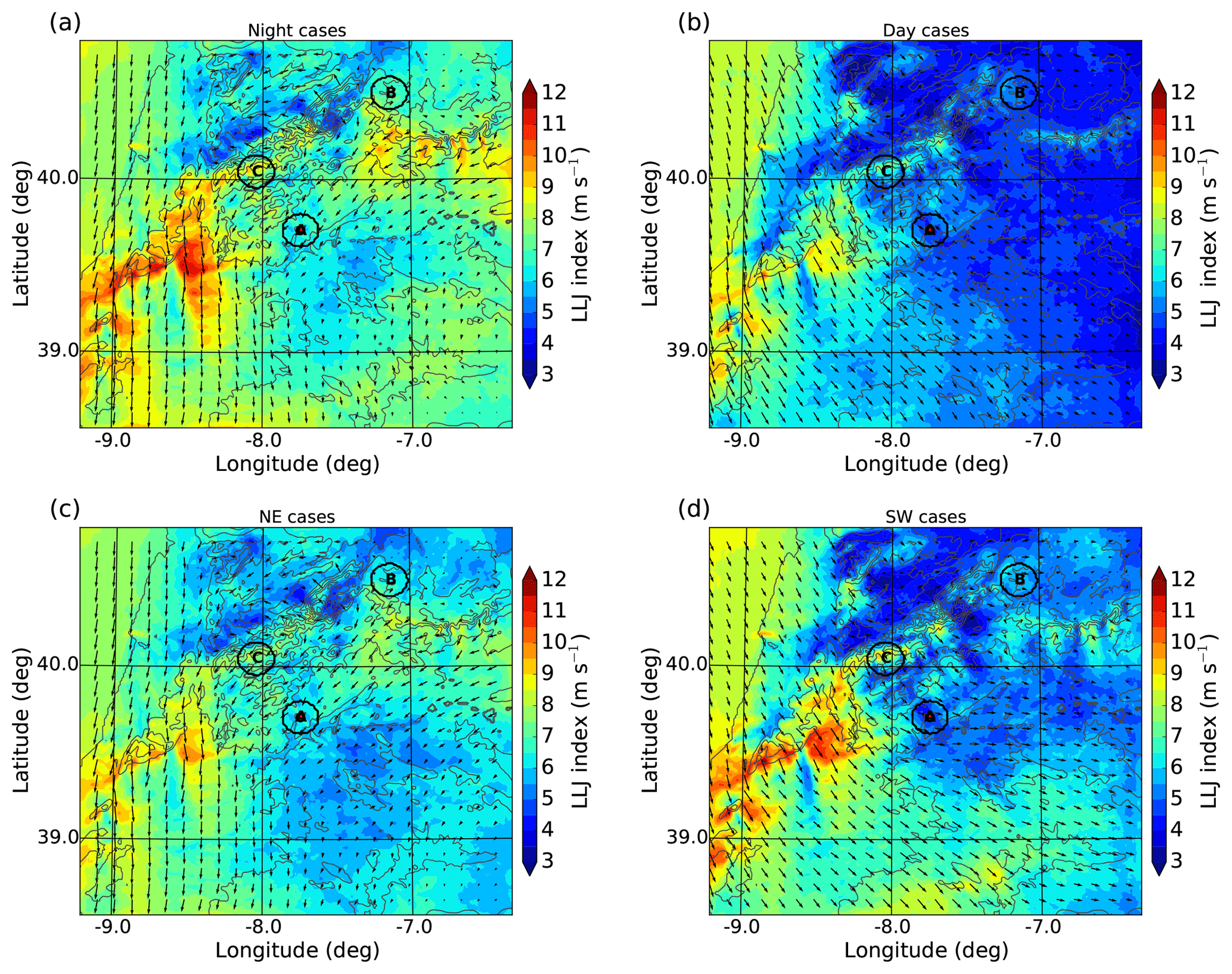
Figure 10Temporal average of the LLJ index for the period 1 May to 15 June 2017. LLJs are detected by comparing wind speeds at 300 and 2000 m a.g.l. during (a) nighttime (21:00 to 09:00 UTC) and (b) daytime (09:00 to 21:00 UTC). In panels (c) and (d), only cases with wind directions from the NE (negative cross-valley winds) and SW (positive cross-valley winds) at 300 m a.g.l. at the location of the WT were used. Arrows show the mean wind field at 300 m a.g.l. during (a) nighttime, (b) daytime, (c) NE and (d) SW LLJ cases. Wind vectors are plotted on every 10th grid point. Areas marked by black circles and letters A to C indicate regions used for the computation of pressure and temperature gradients in cross- and along-valley directions (see text). Region A is centred at the location of the WT. The topography is indicated with thin black contour lines. Data are based on WRF domain D2.
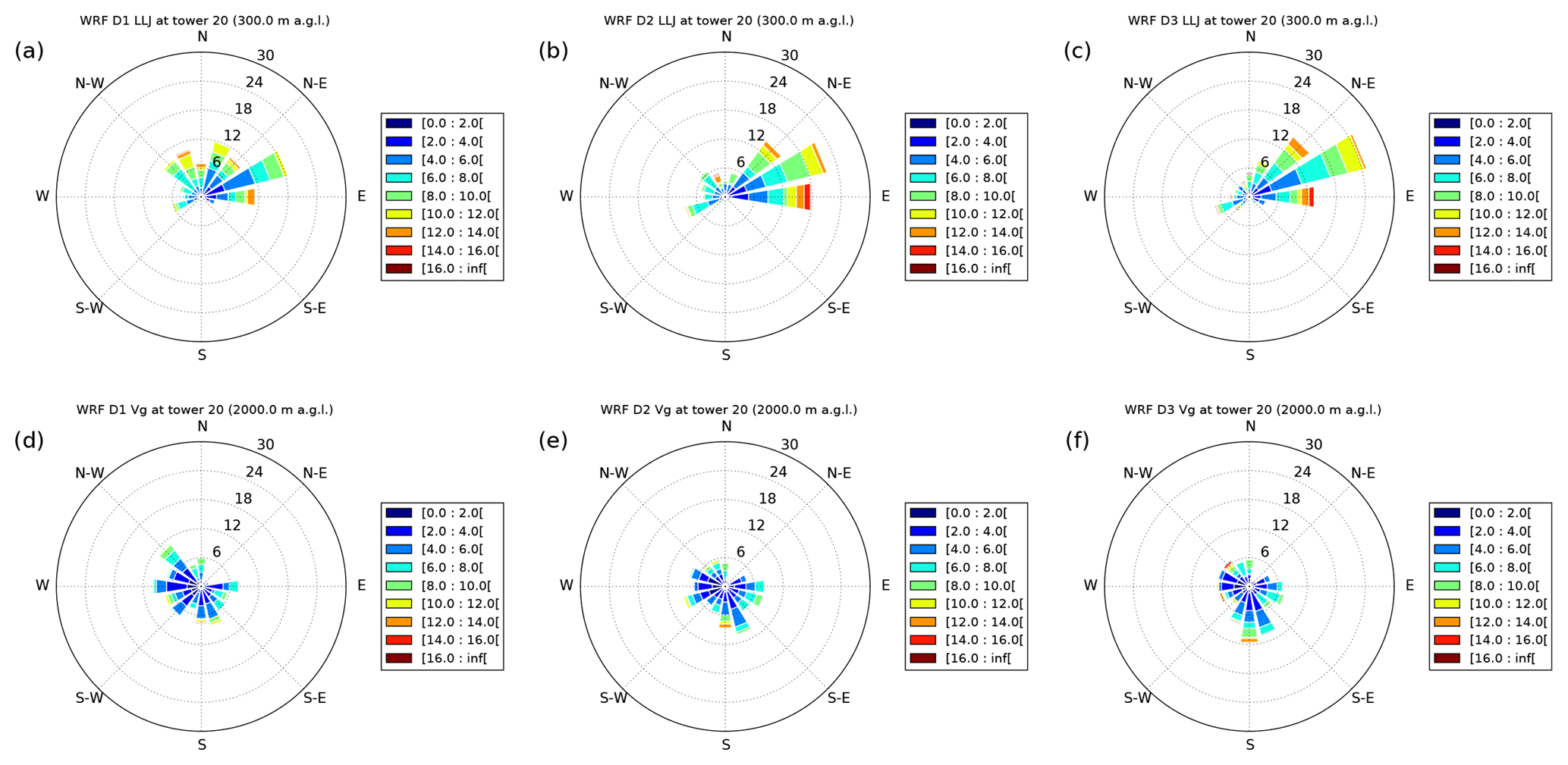
Figure 11Distribution of winds during LLJ events at (a–c) L1 (300 m a.g.l.) and at (d–f) L2 (2000 m a.g.l.) at the location of tower T20 for domains D1 to D3.
In contrast to Rife et al. (2010), our LLJ index is just based on wind speed differences between levels L1 and L2 and not on wind speed differences between night and day. This enables to compute the index for each hour of the day and compare LLJ indices during day- and nighttime. Because of measured evidence and due to a higher horizontal and vertical grid resolution, shallow LLJs are well represented in our model set-up, and we therefore defined the levels L1 and L2 at lower altitudes than Rife et al. (2010), who used L1=500 m a.g.l. and L2=4000 m a.g.l. with a horizontal model grid resolution of 4 km on 28 vertical levels. Figure 10a and b show temporal averages of the LLJ index for the period 1 May to 15 June 2017 for night- and daytime. The computation of nighttime LLJ indices was based on averaging times between 21:00 to 09:00 UTC, while daytime indices were averaged between 09:00 and 21:00 UTC. This classification was used as nocturnal LLJs were often observed to persist until after sunrise, while thermally driven winds from the SW were observed until about 21:00 UTC. Note that local time in Portugal is UTC + 1 h during the summer season. The spatial distribution of nocturnal LLJs in Fig. 10a shows that the strongest nocturnal LLJs develop SW of Perdigão with a strong northerly flow down the slopes of the Serra da Estrela mountains towards the flat Tejo basin. In addition, strong jet winds developed NE of Perdigão over the slopes between the Serra da Estrela and the Sierra de Gata mountain ranges and flowed down the basin of Castelo Branco (see Fig. 1b) as a drainage flow towards the double ridge of Perdigão. Over the sea, there is also a significant LLJ-index signal with mean winds from the north. This flow is associated with the Azores anticyclone, which induces northerly winds parallel to the Portuguese coastline. During the day, the LLJ activity is strongly reduced NE of Perdigão, as can be seen in Fig. 10b. SW of Perdigão and over the ocean, the LLJ index remains as strong as during the night. In these regions, winds are blowing more from the NW direction during the day compared to northerly winds during the night. This is probably due to the sea breeze effect, which adds an onshore wind component to the flow.
As the dominant wind directions for Perdigão are NE and SW, we additionally computed the mean LLJ index for cases when the cross-valley wind at the location of tower T20 next to the WT was negative at 300 m a.g.l. (NE cases) and for cases when it was positive (SW cases). The corresponding LLJ-index maps are shown in Fig. 10c and d. The spatial distribution of LLJs and the mean flow pattern during NE and SW cases are nearly identical to those during night and day cases, respectively (Fig. 10a and b). This is confirmed by a correlation coefficient of 0.92 for the pointwise comparison of night and NE LLJ indices and by a correlation coefficient of 0.90 for daytime and SW cases. This indicates that, on average, LLJs from the NE and SW over the double ridge were respective night- and daytime phenomena, although exceptional cases with nighttime LLJs from the SW have also been observed (Wildmann et al., 2018a). The spatial distribution of LLJ winds at L1 (300 m a.g.l.) is plotted for location T20 in Fig. 11a to c for D1 to D3. Nearly all LLJ cases exhibit NE wind directions and have their origin over the slopes between the Serra da Estrela and Sierra de Gata mountain ranges (see Fig. 10a, c). LLJs from the SW are rare events. The LLJ distribution for D2 is very similar to that for D3. For D1, LLJs are considerably weaker and there is a larger spread of wind directions. In Fig. 11d–f, the distribution of winds during LLJ events at L2 (2000 m a.g.l.) is shown at the location of T20. These winds can be regarded as geostrophic background winds in the free atmosphere and indicate very calm conditions during LLJ events. Winds are quite regularly distributed between directions from the SE to NW, which means that they were decoupled from the boundary layer and cannot be the main driving mechanism for the LLJs near the surface.

Figure 12LLJ indices obtained from (a) RS launches and (b) WP measurements during the campaign. WRF D3 indices were obtained by interpolating data in space and time on the radiosonde flight track and on the wind profiler location. Indices were averaged over the whole campaign period (ALL), the night- and daytime (NIGHT, DAY) and for cases with wind directions from the NE (negative) and SW (positive cross-valley winds at 300 m a.g.l.). The nocturnal index according to the computation of Rife et al. (2010) is labelled with RIFE. The black bars indicate the frequency of LLJ occurrence during all, night-/daytime and NE/SW cases, respectively. For RIFE, the black bars indicate the occurrence of nocturnal jets during the whole campaign. See Fig. 1 for the wind profiler location and the launch site for soundings (every 6 h).
LLJ indices were also computed for all RS and WP measurements during the campaign. WRF D3 data were interpolated in space and time on the RS flight track and on the WP location before the LLJ index was calculated according to Eq. (4). Figure 12 shows the direct comparison of simulated and observed mean LLJ indices, which were averaged for all, night-/daytime and NE/SW cases, respectively. Both RS and WP data indicate that LLJs were strongest during nighttime and during NE cases. The same result is obtained from WRF D3 simulations whose indices agree well with RS and WP observations. LLJ events occurred during 30.0 % (WRF: 23.5 %) of all RS observations and during 17.4 % (WRF: 21.9 %) of all WP observations during the campaign. Winds from the NE at 300 m a.g.l. (L1) were observed during 49.5 % (WRF: 55.0 %) of RS and during 42.0 % (WRF: 55.1 %) of WP measurements. The observed LLJ frequency for NE cases was higher for RS observations (35 %, WRF: 32 %) compared to WP data (23 %, WRF: 26 %), as RSs were launched within the valley (see Fig. 1), while the WP was located on the lee side of the double ridge. At tower T20, which is located on the SW ridge, LLJs did occur more frequently due to the elevated position during 42 % of NE cases and during 30 % of all synoptic conditions in the WRF D3 simulation (not shown). The original nocturnal NLLJ index of Rife et al. (2010) (Eq. 1) was also computed and is labelled with RIFE in Fig. 12. NLLJ values are slightly higher compared to our mean LLJ indices probably as only one value per day is computed for NLLJ indices by comparing the situation at 00:00 and 12:00 UTC (see Eqs. 1 to 3). This results in a lower number of LLJ events and a reduced smoothing when averaging is done over the whole campaign period. This can maybe explain the extreme high WRF NLLJ index at the WP location.
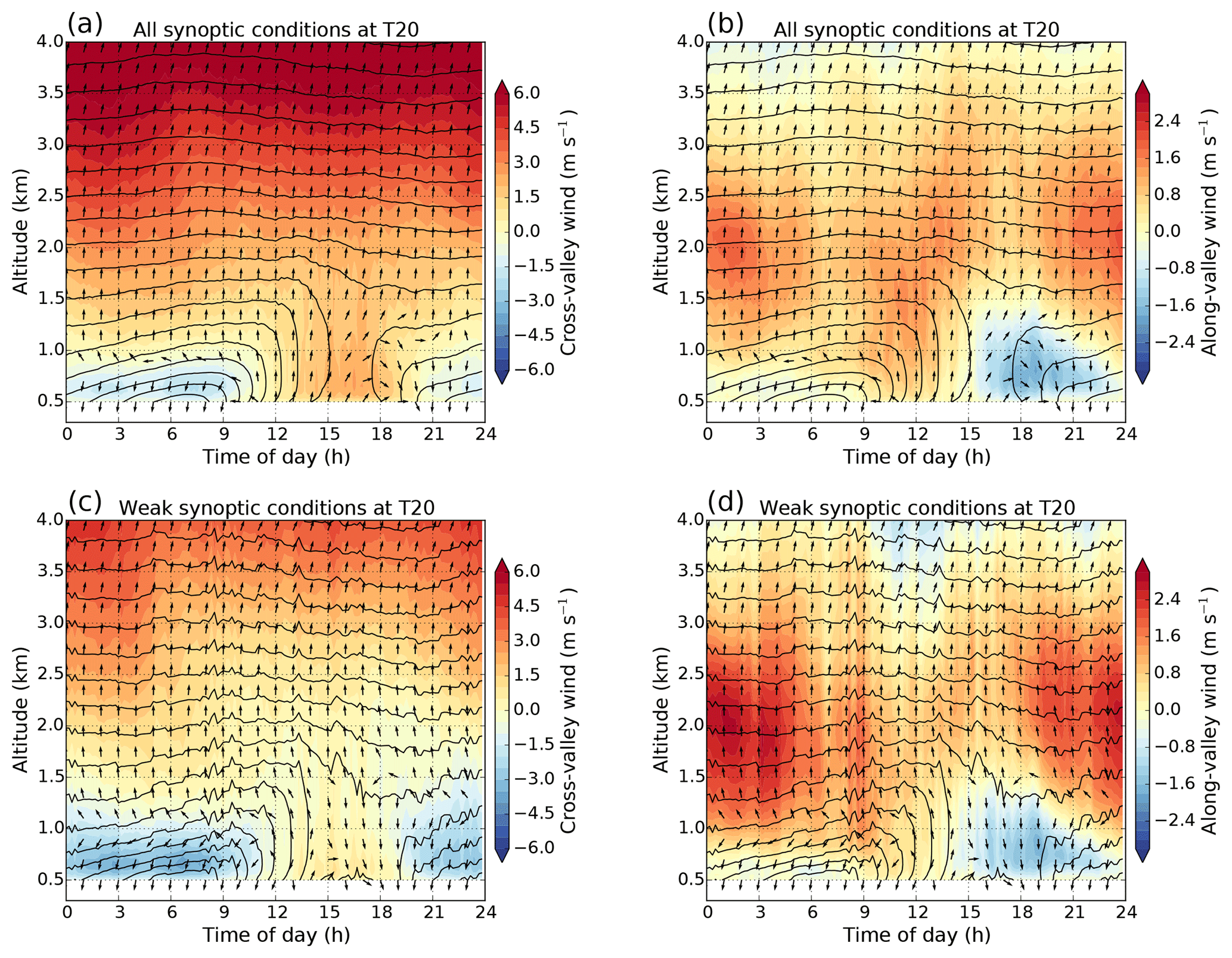
Figure 13WRF D3 mean diurnal vertical profiles of (a, c) cross- and (b, d) along-valley winds at tower T20. The averaging period was 1 May to 15 June 2017. In panels (a) and (b), all data of this period were used for averaging, while in panels (c) and (d), only cases with weak synoptic conditions (defined by horizontal wind speeds <10 m s−1 at 3000 m altitude) were utilized. Negative cross- (along-)valley winds indicate flow from the NE (NW) directions, respectively. Black arrows show the mean horizontal wind direction (north is indicated at the top). Black contour lines mark isentropes with a contour interval of 1 K.
To illustrate the daily changing flow patterns over the double ridge in more detail, we plotted the simulated mean diurnal cycle of cross- and along-valley wind vertical profiles at the location of tower T20 in Fig. 13. In Fig. 13a–b, averaging was done over the whole IOP from 1 May to 15 June 2017, and in Fig. 13c–d only for weak synoptic conditions. The latter were defined if the horizontal wind speed at an altitude of 3000 m was smaller than 10 m s−1 to reduce the effect of synoptic forcing on LLJ development. Cross-valley winds show a strong signal of nocturnal LLJs starting at about 21:00 UTC from northern directions and with a maximum intensity between 06:00 and 09:00 UTC from the NE direction. During the day, a well-mixed PBL develops and mean winds turn to S and SW directions. During daytime, no LLJ structure is recognizable in the mean cross-valley wind. The most interesting feature in the mean along-valley wind profiles is the wind component from the NW (negative values) developing during the evening transition starting at about 15:00 UTC with a maximum between 18:00 and 21:00 UTC. This flow structure is induced by downslope winds, which are generated after sunset over the steep slopes of the Serra da Estrela mountains NW of Perdigão (see Fig. 1b). In the course of the night, the flow over Perdigão turns from a NW to a N and a NE flow due to the developing down-valley LLJ along the Castelo Branco basin (see Fig. 10a). During the morning transition, a SE flow develops into a S and SW flow during the day due to upslope and up-valley winds along the Serra da Estrela mountain slopes and along the Castelo Branco basin, respectively. This results in a clockwise diurnal wind turning near the surface.
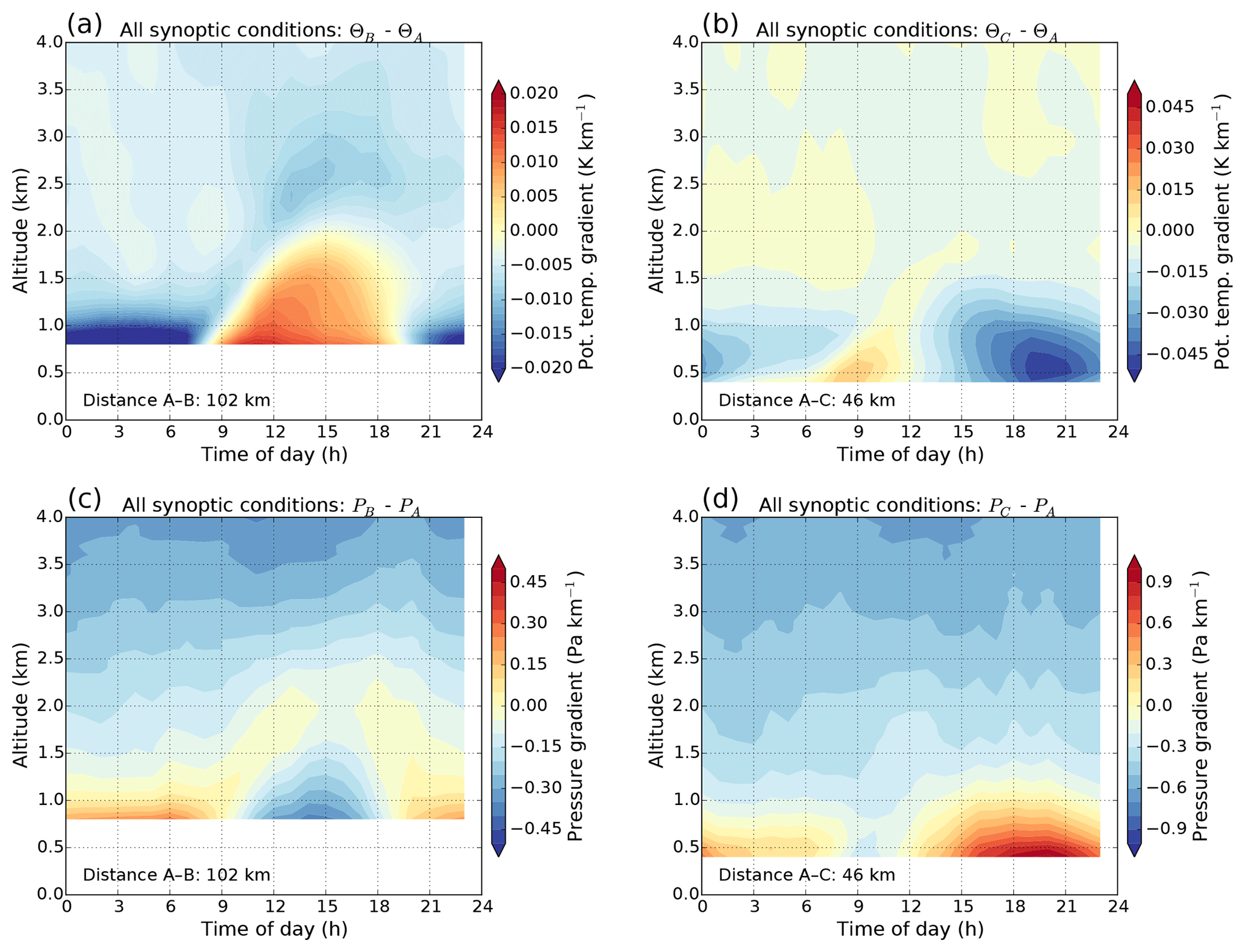
Figure 14WRF D2 mean diurnal vertical profiles of horizontal potential temperature Θ and pressure P gradients between (a, c) regions A and B and (b, d) regions A and C. The locations of the regions are marked in Fig. 10. The averaging period was 1 May to 15 June 2017.
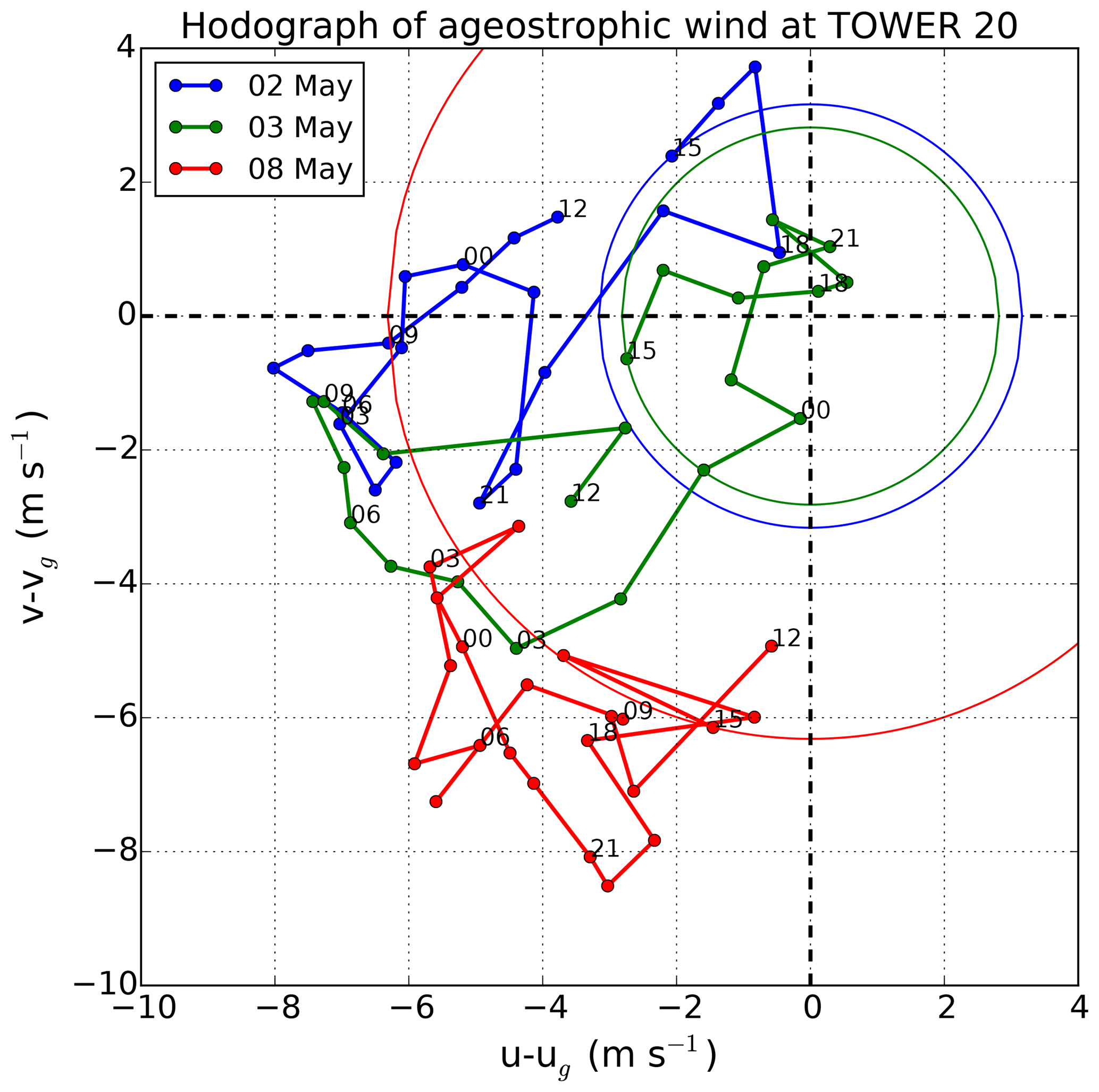
Figure 15WRF D3 hodographs of ageostrophic wind components for three different nocturnal LLJ cases (2, 3 and 8 May 2017) at tower T20. Ageostrophic wind components correspond to differences between winds at level L1 and level L2. Numbers indicate the time of the day in hours. Hodographs start at 15:00 UTC the day before the LLJ case, respectively (e.g. at 15:00 UTC on 1 May for the 2 May case). The theoretical inertial oscillations of the ageostrophic wind according to Blackadar (1957) are illustrated with circles for the respective winds at 15:00 UTC.
To prove our hypothesis that the diurnal flow structures over Perdigão were thermally driven and not an inertial oscillation phenomenon according to the theory of Blackadar (1957), we computed horizontal gradients of potential temperature Θ and pressure in cross- and along-valley directions. Three circular regions were defined in Fig. 10 with diameters of 20 km that were centred at the wind turbine (region A), on the plateau between the Serra da Estrela and Sierra de Gata mountains (region B) and on the steep slopes of the Serra da Estrela mountain range NW of Perdigão (region C). For each region, time series of mean vertical potential temperature and pressure profiles were calculated, which were then used to compute horizontal gradients between regions A–B and regions A–C. Mean diurnal vertical profiles of these gradients are shown in Fig. 14 averaged over the whole campaign period. The difference of Θ between regions A and B shows higher temperatures between about 09:00 and 19:00 UTC and lower temperatures during the night over the elevated plateau in region B (Fig. 14a). This can be explained by the valley volume effect (e.g. Wagner, 1938; Whiteman, 2000) and intensified heating/cooling of the PBL over mountain slopes compared to the background atmosphere (Whiteman, 2000). This topographically induced differential warming/cooling leads to a horizontal pressure gradient, which is shown in Fig. 14c for regions A–B and forces a thermally driven SW flow (higher pressure in region A) during the day and a NE flow (higher pressure in region B) during the night. A similar but a phase-shifted thermally driven flow system can be observed in the along-valley direction when comparing regions A–C in Fig. 14b and d. In the late afternoon, the PBL over the steep slopes in region C is cooled and downslope winds from the NW direction develop. The positive pressure gradient remains throughout the night and changes sign when the PBL is heated over the mountain slopes in region C after sunrise (Fig. 14d). The shown diurnal variation of horizontal pressure gradients is in contrast to the inertial oscillation LLJ theory of Blackadar (1957). A crucial component of this theory is the existence of a non-vanishing synoptic pressure gradient (e.g. Shapiro and Fedorovich, 2009). During the evening transition, a stable boundary layer develops and a LLJ forms due to the sudden reduction of surface friction (Blackadar, 1957; Emeis, 2013). The new balance of pressure gradient and Coriolis force induces a clockwise inertial oscillation of the ageostrophic wind component in time. In Fig. 15, a hodograph of the ageostrophic wind components is plotted for three typical LLJ cases at T20, which occurred on 2, 3 and 8 May 2017 over Perdigão. The hodograph does not show the circular oscillation around the zero point that is typical for the theory of Blackadar (1957). Nearly all points indicate negative ageostrophic wind components, which means that the wind direction of the LLJs is opposite to the geostrophic wind most of the time. This is confirmed by wind roses of LLJs and winds in the free atmosphere in Fig. 11. It is also in agreement with Fig. 14c and d, which show a positive nocturnal pressure gradient near the surface and a relatively constant weak negative synoptic pressure gradient above 2.5 km altitude in the free atmosphere. Another hint that the inertial oscillation theory cannot be the main driving mechanism for Perdigão concerns LLJ peak winds that exceed the geostrophic wind by more than 100 % (Shapiro and Fedorovich, 2009). This is not possible for inertial oscillations but was detected in 26 % of WRF D3 LLJ cases at T20. This analysis and the good agreement between temperature, pressure and wind patterns in Figs. 13 and 14 confirm the dominance of thermally driven flows during the field campaign.
Long-term WRF-LES simulations were performed with a horizontal resolution of 200 m for a period of 49 days during the Perdigão campaign in May and June 2017. Simulation results were used to characterize the meteorological conditions and to analyse characteristic flow patterns during the IOP. The high grid resolution of 200 m was necessary to resolve the double-ridge topography. The realistic computation of turbulence features was not the focus of this paper. Large parts of the campaign were dominated by synoptically calm conditions and the evolution of thermally driven flow systems (especially during the second half of the campaign). On the basis of the frequent observation of LLJs by lidar and in situ measurements, a LLJ index was computed following the method of Rife et al. (2010) to show that nocturnal LLJs from the NE predominantly developed over the steep slopes between the Portuguese Serra da Estrela and the Spanish Sierra de Gata mountain ranges. This katabatic flow intensified during the night and moved down the broad basin of Castelo Branco towards the double-ridge site of Perdigão. During the day, SW winds dominated. Due to the well-mixed PBL, this flow had no LLJ character in most cases. The computation of mean daily cycles of wind direction and cross-valley wind at T20 showed a diurnal clockwise wind turning near the surface with nocturnal LLJs from the NE, S and SW directions during the day and NW and N flow in the evening transition due to downslope winds from the northern Serra da Estrela mountain range. This wind turning was also measured by in situ and lidar instruments. The computation of potential temperature and pressure gradients in cross- and along-valley directions confirmed the hypothesis that PBL flows were mainly thermally driven during the campaign period. LLJ generation according to the inertial oscillation theory of Blackadar (1957) did not play a major role due to weak synoptic forcing, opposite pressure gradients in the PBL and in the free atmosphere and missing circular temporal evolution of ageostrophic winds in the LLJ layer.
The verification of the model with in situ observations showed a surprisingly good agreement in spite of the long simulation horizon of 49 days. Especially the diurnally changing flow from the NE during the night and from the SW during the day was captured well on the ridges of the double hill by all model domains. This indicates that the mesoscale mountain wind system is generally resolved by a model run with 5 km horizontal grid size. The realistic simulation of the interaction of the flow with the complex topography requires, however, a higher resolution of at least 200 m. In the valley, observations showed that along-valley winds were the dominating flow regime. WRF D3 simulations computed these along-valley winds but underestimated the strength of this flow considerably. The reason for this underestimation is not clear. The introduction of turbulence, e.g. by cell perturbation, as well as better land-use data sets including improved roughness and forest maps and enhanced soil moisture data will likely help to simulate the small scales of valley flows in Perdigão more realistically. This has to be tested in further sensitivity runs. The usage of additional roughness elements, such as the applied forest parameterization, will definitely be necessary for future real-case LES simulations.
WRF data are provided for domains 1 to 3 as vertical profile time series at the locations of the 100 m towers T20, T25 and T29 (DLR Institut für Physik der Atmosphäre – WRF long-run, 2019). Observations are provided by NCAR for the wind profiler data (UCAR/NCAR – Earth Observing Laboratory, 2017), the sounding data (UCAR/NCAR – Earth Observing Laboratory, 2018b) and the tower data (UCAR/NCAR – Earth Observing Laboratory, 2018a).
JW performed the numerical simulations; NW and TG participated in the field campaign and conducted the DLR lidar measurements. KG contributed to the analysis of thermally driven flows. JW prepared the paper with contributions from all co-authors.
The authors declare that they have no conflict of interest.
This article is part of the special issue “Flow in complex terrain: the Perdigão campaigns (ACP/WES/AMT inter-journal SI)”. It does not belong to a conference.
This work was performed within the project LIPS, funded by the Federal Ministry of Economy and Energy on the basis of a resolution of the German Bundestag under the contract no. 0325518.
We thank José Laginha Palma, University of Porto, José Carlos Matos
and the INEGI team, as well as the research groups from DTU and NCAR for the
successful collaboration and realization of the Perdigão campaign.
Additionally, we thank the municipalities of Alvaiade and Vila Velha de
Rodão in Portugal for local support. Radiosonde, tower and wind profiler
data were kindly provided by NCAR. We appreciate constructive comments on the
manuscript by Roland Eichinger and two anonymous reviewers.
The article processing charges for this open-access
publication were covered by a Research
Centre
of the Helmholtz Association.
Edited by:
José Laginha Palma
Reviewed by: two anonymous referees
Banta, R. M., Darby, L. S., Fast, J. D., Pinto, J. O., Whiteman, C. D., Shaw, W. J., and Orr, B. W.: Nocturnal low-level jet in a mountain basin complex. Part I: Evolution and effects on local flows, J. Appl. Meteor., 43, 1348–1365, https://doi.org/10.1175/JAM2142.1, 2004. a
Blackadar, A. K.: Boundary Layer Wind Maxima and Their Significance for the Growth of Nocturnal Inversions, B. Am. Meteorol. Soc., 38, 283–290, 1957. a, b, c, d, e, f
Chen, F. and Dudhia, J.: Coupling an advanced land surface-hydrology model with the Penn State-NCAR MM5 modeling system. Part I: Model implementation and sensitivity, Mon. Weather Rev., 129, 569–585, https://doi.org/10.1175/1520-0493(2001)129<0569:CAALSH>2.0.CO;2, 2001. a
Daniels, M. H., Lundquist, J. K., Mirocha, J. D., Wiersema, D. J., and Chow, F. K.: A new vertical grid nesting capability in the Weather Research and Forecasting (WRF) model, Mon. Weather Rev., 144, 3725–3747, https://doi.org/10.1175/MWR-D-16-0049.1, 2016. a
Deardorff, J. W.: Stratocumulus-capped mixed layers derived from a 3-dimensional model, Bound.-Lay. Meteorol., 18, 495–527, https://doi.org/10.1007/BF00119502, 1980. a
DLR Institut für Physik der Atmosphäre – WRF long-run: Long-term simulation of the boundary layer flow over the double-ridge site during the Perdigão 2017 field campaign: WRF time series at locations of 100 m towers, DLR Institut für Physik der Atmosphäre, DLR Oberpfaffenhofen, Germany, https://doi.org/10.5281/zenodo.2539487, 2019. a, b
Dudhia, J.: Numerical study of convection observed during the winter monsoon experiment using a mesoscale two-dimensional model, J. Atmos. Sci., 46, 3077–3107, https://doi.org/10.1175/1520-0469(1989)046<3077:NSOCOD>2.0.CO;2, 1989. a
Emeis, S.: Wind energy meteorology: Atmospheric physics for wind power generation, Springer, Berlin, Heidelberg, 2013. a, b
Fernando, H. et al.: The Perdigão: Peering into microscale details of mountain winds, B. Am. Meteorol. Soc., in press, https://doi.org/10.1175/BAMS-D-17-0227.1, 2018. a, b
Hong, S.-Y. and Lim, J.-O. J.: The WRF single-moment 6-class microphysics scheme (WSM6), J. Korean Meteor. Soc., 42, 129–151, 2006. a
Hong, S.-Y., Dudhia, J., and Chen, S.-H.: A revised approach to ice microphysical processes for the bulk parameterization of clouds and precipitation, Mon. Weather Rev., 132, 103–120, https://doi.org/10.1175/1520-0493(2004)132<0103:ARATIM>2.0.CO;2, 2004. a
Hong, S.-Y., Noh, Y., and Dudhia, J.: A new vertical diffusion package with an explicit treatment of entrainment processes, Mon. Weather Rev., 134, 2318–2341, https://doi.org/10.1175/MWR3199.1, 2006. a
Kain, J. S. and Fritsch, J. M.: A one-dimensional entraining/ detraining plume model and its application in convective parameterization, J. Atmos. Sci., 47, 2784–2802, https://doi.org/10.1175/1520-0469(1990)047<2784:AODEPM>2.0.CO;2, 1990. a
Klemp, J. B., Dudhia, J., and Hassiotis, A. D.: An upper gravity-wave absorbing layer for NWP applications, Mon. Weather Rev., 136, 3987–4004, https://doi.org/10.1175/2008MWR2596.1, 2008. a
Mann, J., Angelou, N., Arnqvist, J., Callies, D., Cantero, E., Chávez Arroyo, R., Courtney, M., Cuxart, J., Dellwik, E., Gottschall, J., Ivanell, S., Kühn, P., Lea, G., Matos, J. C., Palma, J. M. L. M., Pauscher, L., Peña, A., Sanz Rodrigo, J., Söderberg, S., Vasiljevic, N., and Veiga Rodrigues, C.: Complex terrain experiments in the New European Wind Atlas, Phil. Trans. R. Soc., 375, 20160101, https://doi.org/10.1098/rsta.2016.0101, 2017. a
Mlawer, E. J., Taubman, S. J., Brown, P. D., Iacono, M. J., and Clough, S. A.: Radiative transfer for inhomogeneous atmospheres: RRTM, a validated correlated-k model for the longwave, J. Geophys. Res., 102, 16663–16682, https://doi.org/10.1029/97JD00237, 1997. a
Monaghan, A., Rife, D. L., Pinto, J. O., Davis, C. A., and Hannan, J. R.: Global precipitation extremes associated with diurnally varying low-level jets, J. Climate, 23, 5065–5084, https://doi.org/10.1175/2010JCLI3515.1, 2010. a
Muñoz-Esparza, D. and Kosović, B.: Generation of Inflow Turbulence in Large-Eddy Simulations of Nonneutral Atmospheric Boundary Layers with the Cell Perturbation Method, Mon. Weather Rev., 146, 1889–1909, https://doi.org/10.1175/MWR-D-18-0077.1, 2018. a
Muñoz-Esparza, D., Lundquist, J. K., Sauer, J. A., Kosović, B., and Linn, R. R.: Coupled mesoscale-LES modeling of a diurnal cycle during the CWEX-13 field campaign: From weather to boundary-layer eddies, J. Adv. Model. Earth Sy., 9, 1572–1594, https://doi.org/10.1002/2017MS000960, 2017. a, b
Pineda, N., Jorba, O., Jorge, J., and Baldasano, J. M.: Using NOAA AVHRR and SPOT VGT data to estimate surface parameters: application to a mesoscale meteorological model, Int. J. Remote Sens., 25, 129–143, https://doi.org/10.1080/0143116031000115201, 2004. a
Rife, D. L., Pinto, J. O., Monaghan, A. J., Davis, C. A., and Hannan, J. R.: Global distribution and characteristics of diurnally varying low-level jets, J. Climate, 23, 5041–5064, https://doi.org/10.1175/2010JCLI3514.1, 2010. a, b, c, d, e, f, g
Schmugge, T. J., Abrams, M. J., Kahle, A. B., Yamaguchi, Y., and Fujisada, H.: Advanced spaceborne thermal emission and reflection radiometer (ASTER), P. Soc. Photo-Opt. Ins., 4879, https://doi.org/10.1117/12.469693, 2003. a
Schulz, C., Klein, L., Weihing, P., Lutz, T., and Krämer, E.: CFD studies on wind turbines in complex terrain under atmospheric inflow conditions, J. Phys. Conf. Ser., 524, 012134, https://doi.org/10.1088/1742-6596/524/1/012134, 2014. a
Shapiro, A. and Fedorovich, E.: Nocturnal low-level jet over a shallow slope, Acta Geophy., 57, 950–980, https://doi.org/10.2478/s11600-009-0026-5, 2009. a, b
Shaw, T. H. and Schumann, U.: Large-eddy simulation of turbulent flow above and within a forest, Bound.-Lay. Meteorol., 61, 47–64, https://doi.org/10.1007/BF02033994, 1992. a
Skamarock, W. C., Klemp, J. B., Dudhia, J., Gill, D. O., Barker, D. M., Duda, M. G., Huang, X.-Y., Wang, W., and Powers, J. G.: A description of the Advanced Research WRF Version 3, NCAR technical note, Mesoscale and Microscale Meteorology Division, National Center for Atmospheric Research, Boulder, Colorado, USA, available at: http://www2.mmm.ucar.edu/wrf/users/docs/arw_v3.pdf (last access: 23 January 2019), 2008. a
Storm, B., Dudhia, J., Basu, S., Swift, A., and Giammanco, I.: Evaluation of the Weather Research and Forecasting Model on forecasting low-level jets: Implications for wind energy, Wind Energy, 12, 81–90, https://doi.org/10.1002/we.288, 2009. a
Tian, W., Ozbay, A., Yuan, W., Sarakar, P., and Hu, H.: An experimental study on the performances of wind turbines over complex terrain, in: 51st AIAA Aerospace sciences meeting including the new horizons forum and aerospace exposition, 7–10 January 2013, Grapevine, Texas, USA, 1–14, https://doi.org/10.2514/6.2013-612, 2013. a
UCAR/NCAR – Earth Observing Laboratory: NCAR/EOL Quality Controlled 5-minute ISFS surface flux data, geographic coordinate, tilt corrected, Version 1.0, UCAR/NCAR – Earth Observing Laboratory, https://doi.org/10.26023/ZDMJ-D1TY-FG14, 2018a. a, b
UCAR/NCAR – Earth Observing Laboratory: NCAR/EOL 1290 MHz Wind Profiler NIMA Winds and RASS Data, Version 1.0, UCAR/NCAR – Earth Observing Laboratory, https://doi.org/10.5065/D6RB73BK, 2017. a, b
UCAR/NCAR – Earth Observing Laboratory: NCAR/EOL Quality Controlled Radiosonde Data, Version 2.0, UCAR/NCAR – Earth Observing Laboratory, https://doi.org/10.5065/D6H70DM1, 2018b. a, b
Wagner, A.: Theorie und Beobachtung der periodischen Gebirgswinde, Gerl. Beitr. Geophys., 52, 408–449, 1938. a
Whiteman, C. D.: Mountain meteorology: Fundamentals and applications, Oxford University Press, New York, 2000. a, b
Wildmann, N., Kigle, S., and Gerz, T.: Coplanar lidar measurement of a single wind energy converter wake in distinct atmospheric stability regimes at the Perdigão 2017 experiment, J. Phys. Conf. Ser., 1037, 052006, https://doi.org/10.1088/1742-6596/1037/5/052006, 2018a. a
Wildmann, N., Vasiljevic, N., and Gerz, T.: Wind turbine wake measurements with automatically adjusting scanning trajectories in a multi-Doppler lidar setup, Atmos. Meas. Tech., 11, 3801–3814, https://doi.org/10.5194/amt-11-3801-2018, 2018b. a
The experimental layout is described in detail at https://perdigao.fe.up.pt/ (last access: 22 January 2019).