the Creative Commons Attribution 4.0 License.
the Creative Commons Attribution 4.0 License.
 | 06 Sep 2019
Analysis of total column CO2 and CH4 measurements in Berlin with WRF-GHG
Xinxu Zhao
Stephan Hachinger
Christoph Gerbig
Matthias Frey
Frank Hase
Though they cover less than 3 % of the global land area, urban areas are responsible for over 70 % of the global greenhouse gas (GHG) emissions and contain 55 % of the global population. A quantitative tracking of GHG emissions in urban areas is therefore of great importance, with the aim of accurately assessing the amount of emissions and identifying the emission sources. The Weather Research and Forecasting model (WRF) coupled with GHG modules (WRF-GHG) developed for mesoscale atmospheric GHG transport can predict column-averaged abundances of CO2 and CH4 (XCO2 and XCH4). In this study, we use WRF-GHG to model the Berlin area at a high spatial resolution of 1 km. The simulated wind and concentration fields were compared with the measurements from a campaign performed around Berlin in 2014 (Hase et al., 2015). The measured and simulated wind fields mostly demonstrate good agreement. The simulated XCO2 shows quite similar trends with the measurement but with approximately 1 ppm bias, while a bias in the simulated XCH4 of around 2.7 % is found. The bias could potentially be the result of relatively high background concentrations, the errors at the tropopause height, etc. We find that an analysis using differential column methodology (DCM) works well for the XCH4 comparison, as corresponding background biases are then canceled out. From the tracer analysis, we find that the enhancement of XCH4 is highly dependent on human activities. The XCO2 enhancement in the vicinity of Berlin is dominated by anthropogenic behavior rather than biogenic activities. We conclude that DCM is an effective method for comparing models to observations independently of biases caused, e.g., by initial conditions. It allows us to use our high-resolution WRF-GHG model to detect and understand major sources of GHG emissions in urban areas.
- Article
(7391 KB) - Full-text XML
- BibTeX
- EndNote


The share of greenhouse gas (GHG) emissions released from urban areas has continued to increase as a result of urbanization (IEA, 2008; Kennedy et al., 2009; Parshall et al., 2010; IPCC, 2014). At present 55 % of the global population resides in urban areas (UNDESA, 2014), a number that is projected to rise to 68 % by 2050 (UNDESA, 2018). Meanwhile urban areas cover less than 3 % of the land surface worldwide (Wu et al., 2016) but consume over 66 % of the world's energy (Fragkias et al., 2013) and generate more than 70 % of anthropogenic GHG emissions (Hopkins et al., 2016). Carbon dioxide (CO2) emissions from energy use in cities are estimated to comprise more than 75 % of the global energy-related CO2, with a rise of 1.8 % yr−1 projected under business-as-usual scenarios between 2006 and 2030 (IEA, 2009). Methane (CH4) emissions from energy, waste, agriculture and transportation in urban areas make up approximately 21 % of the global CH4 emissions (Marcotullio et al., 2013; Hopkins et al., 2016). As emission hotspots, urban areas therefore play a vital role in GHG mitigation. It is crucial to find appropriate methods for understanding and projecting the effects of GHG emissions on urban areas and for formulating mitigation strategies.
There are two methods for the quantitative analysis of GHG emissions: the bottom-up approach and the top-down approach (Pillai et al., 2011; Caulton et al., 2014; Newman et al., 2016). The bottom-up approach calculates emissions based on activity data (i.e., a quantitative measure of the activity that can emit GHGs) and emission factors (Wang et al., 2009). This approach has some uncertainty, e.g., on the national fossil-fuel CO2 emission estimates, ranging from a few percent (e.g., 3 %–5 % for the US) to a maximum of over 50 % for countries with fewer resources for data collection and a poor statistical framework (Andres et al., 2012). The considerable uncertainties are caused by the large variability in source-specific and country-specific emission factors and the incomplete understanding of emission processes (Montzka et al., 2011; Bergamaschi et al., 2015). These uncertainties grow larger at subnational scales, when estimating the disaggregation of the national annual totals in space and time. The top-down approach can not only provide estimated global fluxes but also verify the consistency and assess the uncertainties of bottom-up emission inventories (Wunch et al., 2009; Montzka et al., 2011; Bergamaschi et al., 2018). However, it is hard to quantify the statistical errors attached to both atmospheric observations and prior knowledge about the distribution of emissions and sinks (Cressot et al., 2014).
McKain et al. (2012) suggested that column measurements can provide a promising route to improving the detection of CO2 emitted from major source regions, possibly avoiding extensive surface measurements near such regions. Such measurements, i.e., measurements of concentration averaged over a column of air, are performed to help to disentangle the effects of atmospheric mixing from the surface exchange (Wunch et al., 2011) and decrease the biases associated with estimates of carbon sources and sinks in atmospheric inversions (Olsen and Randerson, 2004). Compared to surface values, urban enhancements in columns are less sensitive to boundary-layer heights (Wunch et al., 2011; McKain et al., 2012; Kivi and Heikkinen, 2016), and column observations have the potential to mitigate mixing height errors in an atmospheric inversion system (Gerbig et al., 2008). Atmospheric GHG column measurements combined with inverse models are thus a promising method for analyzing GHG emissions and can be used to analyze their spatial and temporal variability (Ohyama et al., 2009; Pillai et al., 2011; Ostler et al., 2016; Kivi and Heikkinen, 2016).
In order to focus the top-down approach on concentration differences caused by local and regional emission sources, and in particular to quantify urban emissions, the differential column methodology (DCM) was proposed. It evaluates differences between column measurements at different sites. Chen et al. (2016) applied the DCM using the compact Fourier-transform spectrometers (FTSs) EM27/SUN (Bruker Optik, Germany) and demonstrated the capability of differential column measurements for determining urban and local emissions in combination with column models. Citywide GHG column measurement campaigns have been carried out, e.g., in Boston (Chen et al., 2014), Indianapolis (Franklin et al., 2017), San Francisco, Berlin (Hase et al., 2015) and Munich (Chen et al., 2018). However, only a few studies have combined differential column measurements with high-resolution models. Toja-Silva et al. (2017) simulated the column data at upwind and downwind sites of a gas-fired power plant in Munich using the computational fluid dynamic (CFD) model and compared them with the column measurements. Viatte et al. (2017) quantified CH4 emissions from the largest dairies in the southern California region, using four EM27/SUNs in combination with the Weather Research and Forecasting model (WRF) in the large-eddy simulation mode. Vogel et al. (2019) deployed five EM27/SUN spectrometers in the Paris metropolitan area and analyzed the data with the atmospheric transport model framework CHIMERE-CAMS.
This paper carries out a quantitative analysis of GHG for the Berlin area in combination with DCM. We utilize the mesoscale WRF model (Skamarock et al., 2008) coupled with GHG modules (WRF-GHG; Beck et al., 2011) at a high resolution of 1 km. The aim is to assess the precision of WRF-GHG and to provide insights on how to detect and understand sources of GHGs (CO2 and CH4) within urban areas. WRF is a numerical weather prediction system and can be used for both atmospheric research and operational forecasting on a mesoscale range from tens of meters to thousands of kilometers (e.g., Chen et al., 2011). To produce high-resolution regional simulations of atmospheric CH4 passive tracer transport, WRF was coupled with the Vegetation Photosynthesis and Respiration module (WRF-VPRM; Ahmadov et al., 2007). WRF-VPRM has been widely employed in several studies in which both the generally good agreement of the simulations with measurements and model biases were assessed in detail (Ahmadov et al., 2009; Pillai et al., 2011, 2012; Kretschmer et al., 2012). Biogenic carbon fluxes given by the VPRM model tend to underestimate urban ecosystem carbon exchange, owing to the incomplete understanding of urban vegetation and to conditions related to urban heat islands and altered urban phenology (Hardiman et al., 2017). WRF-VPRM was later extended to WRF-GHG (Beck et al., 2011), which can simulate the regional passive tracer transport for GHGs (CH4, CO2 and carbon monoxide – CO). Relatively few studies using WRF-GHG have been published as of yet. Pillai et al. (2016) utilized a Bayesian inversion approach based on WRF-GHG at a high spatial resolution of 10 km for Berlin to obtain anthropogenic CO2 emissions and to quantify the uncertainties in retrieved anthropogenic emissions related to instruments (e.g., CarbonSat) and modeling errors. An observation system simulation experiment was studied in Pillai et al. (2016) based on synthetic data rather than on real observations, as in our study. In the present paper, our focus is on a high-resolution (1 km) study of both CO2 and CH4 in Berlin and assessing the performance of WRF-GHG through comparing the simulated wind and concentration fields to observations from wind stations and ground-based solar-viewing spectrometers. Then DCM is tested as a proper approach for model analysis, which can cancel out the bias from initialization conditions and highlight regional emission tracers. The simulation workflow is also adapted to this purpose where needed. This study is the fundamental study of the WRF-GHG mesoscale modeling framework in urban areas.
The total annual CO2 emissions of Berlin (21.3 million t in 2010) approximately correspond to those of Croatia, Jordan or the Dominican Republic (Reusswig and Lass, 2014). With its strong regulatory influence as a state within Germany, and having a strongly supportive policy, Berlin has already transformed itself into a climate-friendly city in which CO2 emissions have been reduced by a third compared with 1990 levels, aiming for carbon neutrality by 2050 (Homann, 2018). Berlin therefore needs to assess and identify the emission sources accurately at the current stage to provide solid scientific support for the selection of mitigation options. Additionally, Berlin is an ideal pilot case for developing and testing simulations because the city is relatively isolated from other large cities with high emissions, such that anthropogenic GHG anomalies around Berlin can confidently be attributed to the city itself.
The major goals of our work in this context are (1) to simulate high-resolution (1 km) CO2 and CH4 concentrations for Berlin using WRF-GHG, attributing the changes in concentrations to different emission processes, (2) to compare the simulation outputs with the observations from a column measurement network in Berlin (Hase et al., 2015), assessing the precision of WRF-GHG, and (3) to use DCM in the simulation analysis, testing the feasibly of this approach. The structure of this paper is as follows: the model with its domain and external data sources are described in Sect. 2. A comparison analysis for wind fields and concentration fields is presented in Sect. 3, and CO2 and CH4 concentrations related to different processes (e.g., the anthropogenic component) are discussed. DCM, for the comparison of concentration fields and the tracer analysis, is presented and discussed in Sect. 4. Section 5 provides the discussion and summary of this study.
As mentioned in Sect. 1, we use the WRF model version 3.2 coupled with GHG modules to quantify the uptake and emission of atmospheric GHGs around Berlin at a high resolution of 1 km. WRF follows the fully compressible nonhydrostatic Euler equations (Skamarock et al., 2005, 2008) and is based on the actual meteorological data in this case study. The meteorological initial conditions and lateral boundary conditions were taken from the Global Forecast System (GFS) model reanalysis in which in situ measurements and satellite observations were assimilated. Tracers in WRF-GHG are transported online in a passive way, i.e., without any chemical loss or production, when the tracer transport option is used (Ahmadov et al., 2007; Beck et al., 2011). As shown in Fig. 1, three domains are set up here, whose dimensions are 70×50 horizontal grid points with a spacing of 9 km for the coarsest domain (d01), 3 km for the middle domain (d02) and 1 km for the innermost domain (d03). WRF uses a terrain-following hydrostatic pressure vertical coordinate (Skamarock et al., 2008). In our case, 26 vertical levels are defined from the surface up to 50 hPa, 14 of which are in the lowest 2 km of the atmosphere. The innermost domain, d03, envelops all five measurement sites (see Sect. 3.1) to assess the simulation by comparing with the measured data. Berlin lies in the North European Plain on flat land (crossed by northward-flowing watercourses), which avoids the vertical interpolation problems caused by topography differences (Fig. 1). The Lambert conformal conic (LCC) projection is selected as a map projection. The simulated time span is from 18:00 UTC on 30 June to 00:00 UTC on 11 July in 2014. The description of the workflow for running WRF-GHG can be found in Appendix A.
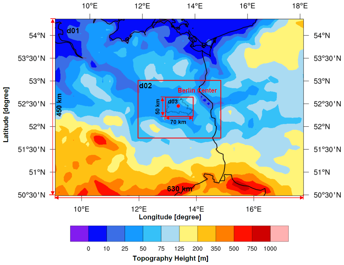
Figure 1The topography map for the three domains in our study. The domain d03 is centered over Berlin, at 13.383° N, 52.517° E, and is marked with a red star. The boundary of Berlin from GADM (available at https://gadm.org/ (last access: 22 July 2019); © GADM maps and data) is depicted in the innermost domain.
The meteorological fields are obtained from the Global Forecast System (GFS) model at a horizontal resolution of 0.5∘, with 64 vertical layers and a temporal resolution of 3 h (as available via the NOAA's National Center for Environmental Information; https://www.ncdc.noaa.gov/, last access: 22 July 2019). The GFS uses hydrostatic equations for the prediction of atmospheric conditions, and its output includes large amounts of atmospheric and land–soil variables, wind fields, temperature, precipitation and soil moisture, etc. The initial and lateral boundary conditions for our WRF-GHG concentration fields are implemented using Copernicus Atmosphere Monitoring Service (CAMS) data (Agusti-Panareda et al., 2017). CAMS provides the estimated mixing ratios of CO2 and CH4, with a spatial resolution of 0.8∘ on 137 vertical levels and with a temporal resolution of 6 h (as available via https://atmosphere.copernicus.eu, last access: 22 July 2019).
The simulation of CO2 and CH4 fluxes with different emission tracers in WRF-GHG is based on flux models and emission inventories which are either already implemented inside the model modules (online calculation) or constitute external datasets (offline calculation). The flux values from external emission inventories are converted into atmospheric concentrations and added to the corresponding tracer variables. In combination with the background concentration fields for CO2 and CH4 that refer to the CO2 and CH4 values without any sources and sinks in the targeted domain, the tracer contributions are summed up to obtain the total concentrations:
where CO2,total and CH4,total represent the total CO2 and CH4, CO2,bgd and CH4,bgd are the background CO2 and CH4, CO2,anthro and CH4,anthro stand for the changes in CO2 from the anthropogenic emissions, CO2,VPRM is the change in CO2 from the biogenic activities and CH4,soil is the change in CH4 from soil uptake, and ΔCO2 and ΔCH4 are the tiny computational errors for CO2 and CH4 that are described in detail in Appendix B. In the transport process, the relationship shown in Eq. (1) holds for each vertical level.
The biogenic CO2 emission is calculated online using VPRM (Mahadevan et al., 2008), in which the hourly Net Ecosystem Exchange (NEE) of CO2 reflects the biospheric fluxes between the terrestrial biosphere and the atmosphere, estimated by the sum of gross ecosystem exchange (GEE) and respiration. VPRM in WRF-GHG calculates biogenic fluxes initialized by vegetation indices (land surface water index – LSWI, enhanced vegetation index – EVI, etc.) from the MODIS satellite (as available via https://modis.gsfc.nasa.gov/, last access: 22 July 2019). The reflectance data from the SYNMAP vegetation classification at a resolution of 1 km and 8 d from the MODIS satellite at 0.5–1 km spatial resolution (depending on the wavelength band) are aggregated onto the LCC projection within the VPRM preprocessor. Then, the data, including the high-solution vegetation indices at a resolution of 1 km, are available on the model domains.
We use the external dataset Emission Database for Global Atmospheric Research version 4.1 (EDGAR V.4.1) for the anthropogenic fluxes in our study. EDGAR V.4.1 provides annually varying global anthropogenic GHG emissions and air pollutants at a spatial resolution of 0.1∘ (Muntean et al., 2014; Janssens-Maenhout et al., 2015), whose source sectors include industrial processes, on-road and off-road sources in transport, large-scale biomass burning, and other anthropogenic sources (Saikawa et al., 2017). Here we apply time factors for seasonal, weekly, daily and diurnal variations defined by the time profiles published on the EDGAR website (http://themasites.pbl.nl/tridion/en/themasites/edgar/documentation/content/Temporal-variation.html, last access: 22 July 2019); however, considerable uncertainties are to be expected in applying these time factors. This temporal variation set is derived based on western European data such that the representativity for other European countries and even other world regions may be quite poor. The coarse emission fluxes used for the initialization of the anthropogenic tracer in WRF-GHG can cause problems when locating emission points within the high-resolution model grid and can weaken the impact from the real high-emission hotspots in the fine domain of our study. The chemical sink for atmospheric CH4 (e.g., photochemistry in the stratosphere) can be ignored in the model, owing to its relatively long lifespan (9.5±1.3 year, Holmes, 2018), the small-scale domains and the limited simulation period (10 d) in our case.
3.1 Description of measurement sites
The measurement campaign used for comparison with WRF-GHG in this paper was performed from 23 June to 11 July 2014 in Berlin using five spectrometers (Hase et al., 2015). It allows us to both test the precision of WRF-GHG (Sect. 3) and verify differential column methodology (DCM) as our analytic methodology (Sect. 4). In their measurement campaign, Hase et al. (2015) used five portable Bruker EM27/SUN FTSs for atmospheric measurements based on solar absorption spectroscopy. Five sampling stations around Berlin were set up, four of which (Mahlsdorf, Heiligensee, Lindenberg and Lichtenrade) were roughly situated along a circle with a radius of 12 km around the center of Berlin. Another sampling site was closer to the city center and located inside the Berlin motorway ring at Charlottenburg (Fig. 6). Detailed information on this measurement campaign is given in Hase et al. (2015), and Frey et al. (2015) provide additional details on the calibration of the spectrometers, precision and instrument-to-instrument biases.
3.2 Comparison of wind fields at 10 m
Winds have a strong impact on the vertical mixing of GHGs and a direct influence on their atmospheric transport patterns. Hence, we firstly compare the wind speeds and wind directions obtained from WRF-GHG to the measurements such that deviations between the simulated and measured wind fields are assessed. The wind measurements are not exactly co-located with the spectrometers mentioned in Sect. 3.1, but are rather located at three sampling sites (Tegel, Schönefeld and Tempelhof) and measure at a height of 10 m above the ground. The simulated wind speed at 10 m (ws10 m) and wind direction at 10 m (wd10 m) are calculated following the equations
where u10 m and v10 m are the components of the horizontal wind, towards the east and north, respectively, which can be obtained from WRF-GHG output files.

Figure 2Variation and differences between simulated and measured wind fields for (a) wind speeds and (b) wind directions from 1 to 10 July 2014 at the three measurement sites, Schönefeld (red lines), Tegel (black lines) and Tempelhof (blue lines), in Berlin. The solid lines represent the simulated wind fields provided by WRF-GHG, and the dashed lines depict the measured wind fields. The differences in (a) and (b) are simulations minus measurements. FTS measurement time periods on each date are marked by gray shaded areas.
Figure 2 shows the comparisons of wind speeds (Fig. 2a) and wind directions (Fig. 2b) between simulations and observations at 10 m from 1 to 10 July and the model–measurement differences. EM27/SUN only operates in the daytime when there is sufficient sunlight; the detailed description of the instrument can be found in Gisi et al. (2012), Frey et al. (2015) and Vogel et al. (2019). The instrumental working periods are marked by gray shaded boxes in Fig. 2. The measured (dashed lines) and simulated (solid) wind speeds (Fig. 2a) at 10 m show similar trends and demonstrate relatively good agreement over the 10 d time series, with a root-mean-square error (RMSE) of 0.9247 m s−1. Large uncertainties in wind speeds are found to appear always with the lower wind speeds, mostly at night. In terms of wind directions at 10 m, we observe that the simulated wind directions show similar but slightly underestimated fluctuations (Fig. 2b), which result in an RMSE of 60.8328∘. Larger uncertainties in wind directions always exist during the low wind speed periods (Fig. 2a, b). During the instrumental working period (within the daytime), the simulations fit better with the measurements with relatively lower RMSEs of 0.6928 m s−1 for wind speeds and 41.4793∘ for wind directions. We find that the measured wind fields (both wind speeds and wind directions) have more fluctuations compared to the simulations. This could be caused by really fast wind changes which the model, simulating a somewhat idealized environment, is not able to capture. To be specific, local turbulence given by urban canopy, buildings, etc., is not represented well in the model.
3.3 Comparison of pressure-weighted column-averaged concentrations
In the following, we use the measured concentration fields to compare with the simulated fields. An FTS EM27/SUN can measure the column-integrated amount of a tracer through the atmospheric column with excellent precision, yielding the column-averaged dry-air mole fractions (DMFs) of the target gases (Chen et al., 2016; Hedelius et al., 2016). The measured DMFs of CO2 and CH4 are denoted by XCO2 and XCH4. Hase et al. (2015) used constant a priori profile shapes in the retrievals of measurements.
When comparing remote sensing observations to model data (or also datasets from different remote sensing instruments to one another), limitations of the instruments in reconstructing the actual atmospheric state need to be taken into account. In general, this requires the a priori profile that is used for the retrieval and the averaging kernel matrix, which specifies the loss of vertical resolution (fine vertical details of the actual trace gas profile cannot be resolved) and limited sensitivity (e.g., Rodgers and Connor, 2003). In the case of EM27/SUN, the spectrometers used in the network offer only a low spectral resolution of 0.5 cm−1. Therefore, performing a simple least-squares fit by scaling retrieval of the a priori profile is generally appropriate. In this case, there is no need to specify a full averaging kernel matrix; instead, the specification of a total column sensitivity is sufficient. The total column sensitivity is a vector (being a function of altitude), which specifies to which degree an excess partial column superimposed on the actual profile at a certain input altitude is reflected in the retrieved total column amount. This sensitivity vector is a function of a solar zenith angle (SZA; and ground pressure), mainly due to the fact that the observed signal levels in different channels building the spectral scene used for the retrieval are shaped by a mixture of weaker and stronger absorptions. (If all spectral lines in the spectral scene are optically thin and too narrow to be resolved by the spectral measurement, the sensitivity would approach unity throughout.)
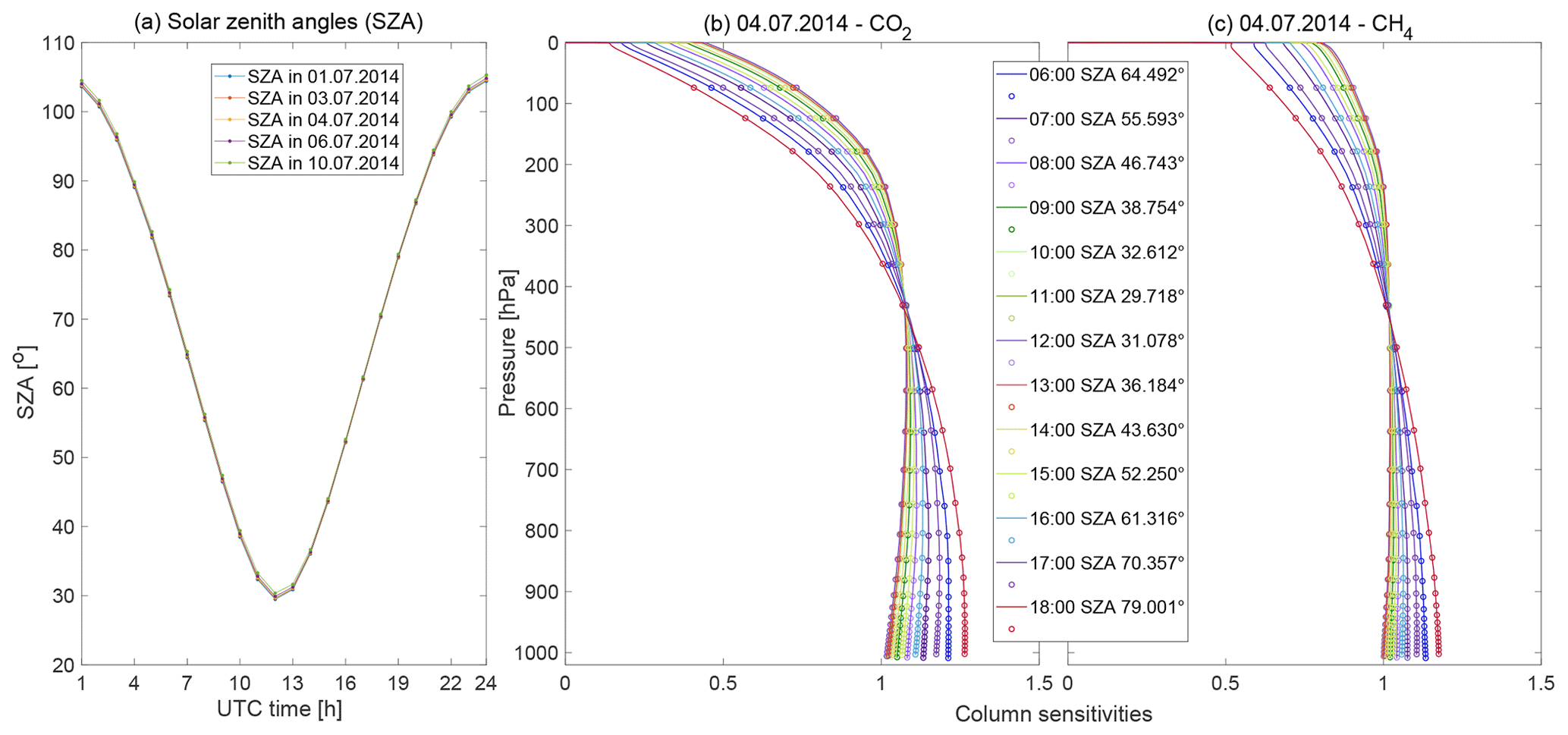
Figure 3(a) Daily variations in solar zenith angle (SZA) for five simulation dates (1, 3, 4, 6 and 10 July), and the vertical distributions of column sensitivities for (b) CO2 and (c) CH4 on 4 July. In (b) and (c), the solid lines represent our derived column sensitivities for EM27/SUN under different SZAs, and the circles stand for the values on model pressure levels.
In order to ensure measurement quality and enough sample points for further concentration comparisons, we select five measurement dates (1, 3, 4, 6 and 10 July) with relatively good measurement qualities (from fair, “++”, to very good, “++++”) based on Hase et al. (2015). The pressure-dependent column sensitivities for CO2 (Fig. 3b) and CH4 (Fig. 3c) are derived from measurements performed in Lindenberg on 4 July (the best-quality day in terms of measurements). Details about the measurements can be found in Hase et al. (2015) and Frey et al. (2015). The shape and values of the column sensitivities from Lindenberg in Berlin closely resemble the results of Hedelius et al. (2016) in Pasadena. As depicted in Fig. 3a, the SZAs are almost identical for each day in our study (at each hour), rendering the shape of column sensitivities (at a specific hour of the day) practically independent of the measurement date. The column sensitivities for 4 July (Fig. 3b, c) are taken as a basis for our smoothing process below. The a priori CO2 and CH4 profiles have been taken from the Whole Atmosphere Community Climate Model (WACCM) version 6. A smoothed profile for a target gas G is then obtained as in Eq. (3) in Vogel et al. (2019),
where G is the modeled profile from WRF-GHG, I is the identity matrix, K is a diagonal matrix containing the averaging kernel and Gp is the a priori profile.
In order to compare the simulated smoothed concentration fields with the observations, the simulated smoothed pressure-weighted column-averaged concentration for a target gas G (XG) is calculated as
Here, Δpi is proportional to the differences of the pressure values P(i) at the bottom and P(i+1) at the top of the ith vertical grid cell, Ptop and Psf represent the hydrostatic pressures at the top and at the surface of the model domain, and Gs(i) stands for the simulated concentration of the target gas G at the ith vertical level.
In Figs. D1 and D2 of Appendix D, we compare the simulated XCO2 and XCH4 with and without smoothing. The simulated concentrations are only slightly enlarged after smoothing, at approximately 1–2 ppm for XCO2 and 2 ppb for XCH4, while the variations are mostly unchanged. Compared to the period with lower SZAs (at noon), the smoothed values in the morning and afternoon with higher SZAs hold relatively larger enlargements.
Figure 4a shows the measured and smoothed modeled variations in XCO2 and XCH4 for these 5 d. Compared to the measurements, the smoothed simulated pressure-weighted column-averaged concentrations for CO2 (XCO2) show quite similar trends but with approximately 1–2 ppm bias, indicated by an RMSE of 1.2534 ppm. The simulated XCO2 values are overestimated for 1, 3 and 4 July, while on 6 and 10 July, the model is underestimated, which could be the result of uncertainties from the coarse anthropogenic surface emission fluxes, background concentrations from CAMS (Sembhi et al., 2015) and the ignorance of the influence from the line of sight of the sun.
Figure 4b shows the comparison of the pressure-weighted column-averaged concentrations for CH4 (XCH4) between observations and smoothed simulations on the five selected dates (1, 3, 4, 6 and 10 July). We find that there is an approximate offset of 50–60 ppb between observations and models (RMSE is 58.1082 ppb). The simulated XCH4 is around 1860 ppb while the measured value is around 1810 ppb, which is comparable to the values (1790–1810 ppb) observed at two Total Carbon Column Observing Network (TCCON) measurement sites in June and July 2014 in Bremen in Germany (Notholt et al., 2014) and Bialystok in Poland (Deutscher et al., 2014). This bias of the simulated XCH4 seems to be constant (around 2.7 %) each day. Thus, we introduce an offset applied to all sites for each simulation date to compare the model and the measured data, effectively removing the bias, which we attribute to too high a background XCH4. The daily offset is assumed to be the difference between the smoothed simulated and measured daily mean XCH4. After applying the daily offset, the measured XCH4 shows a somewhat better agreement and a similar trend but with larger variability compared to the simulation (RMSE is 3.1690 ppb). The smaller variations from the simulation results can, for example, be caused by the error from the spatio-temporal treatment of emission maps, underestimated emissions from anthropogenic activities, the coarse wind data and/or the smoothing of actual extreme values in the simulation.
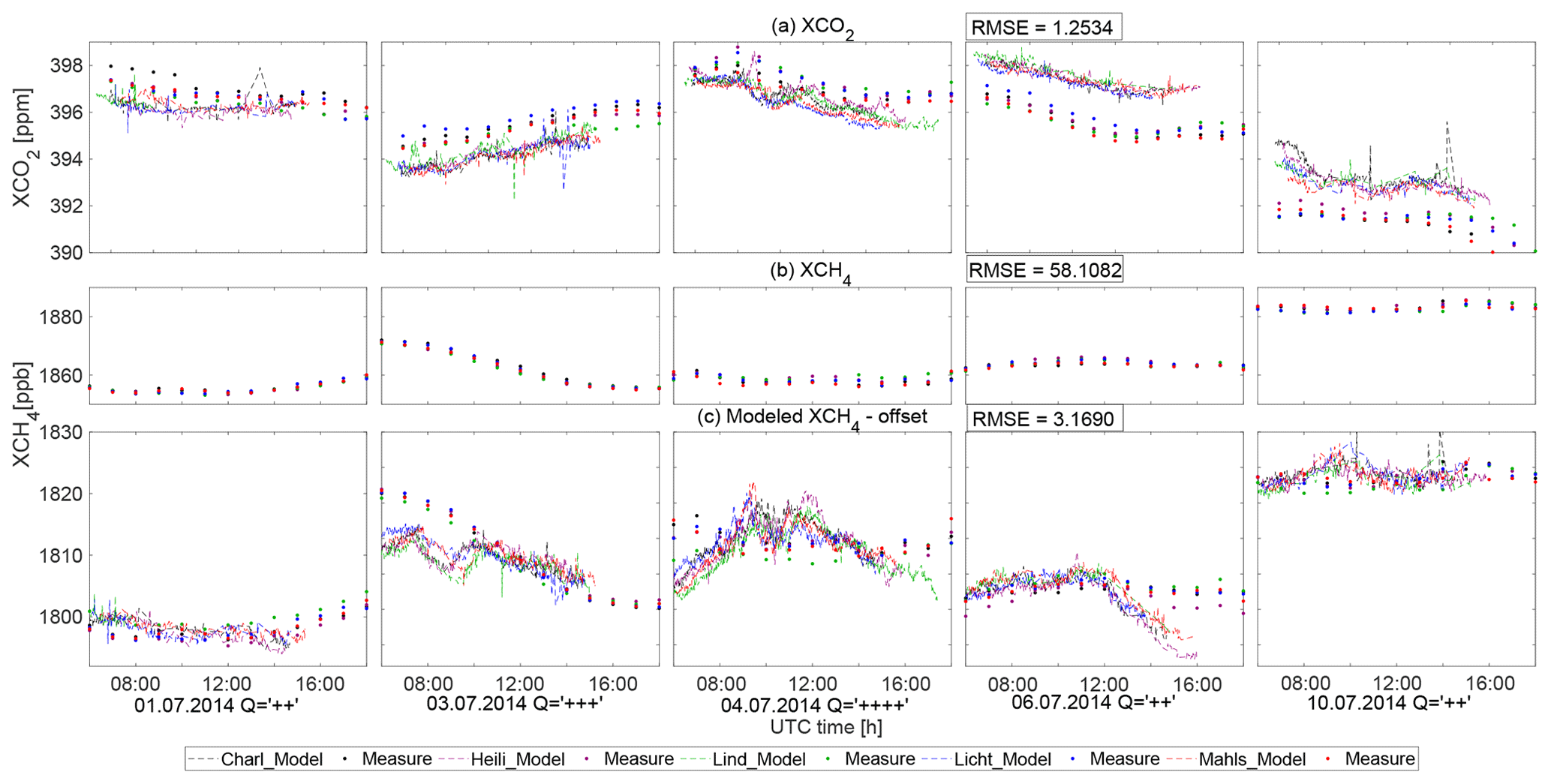
Figure 4Variations of the measured and smoothed simulated (a) XCO2 and (b) XCH4, on 1, 3, 4, 6 and 10 July 2014, for five sampling sites in Berlin: Charlottenburg (Charl: black markers), Heiligensee (Heili: purple markers), Lichtenrade (Licht: green markers), Lindenberg (Lind: blue markers) and Mahlsdorf (Mahls: red markers). The solid circles in (a) and (b) stand for the simulated values provided by WRF-GHG, and the dashed lines represent the measured concentrations. The solid circles represent the simulated XCH4 after the subtraction of the daily offset in (c).
A major offset in modeled CH4 concentration fields could potentially be attributed to the errors in the troposphere height and a general offset from CAMS. In the CH4 vertical concentration profile, we find that the typical sharp decrease occurs at the tropopause height. Tukiainen et al. (2016) also find the similar sharp decrease when using the AirCore to retrieve atmospheric CH4 profiles in Finland. During the simulation, the background concentration values of CAMS are directly fitted to the WRF pressure axis without considering the actual tropopause height; thus this could cause some error. An illustration of the vertical distribution for CH4 is provided in Appendix C. In contrast, the CO2 vertical distribution shows decrease that is quite flat with the increase in pressure, and there is no need to consider the tropopause height during the grid treatment in the vertical layer. In terms of CAMS, the reports from Monitoring Atmospheric Composition and Climate (MACC) stated that CAMS has a bias and RMSE (approximately 50 ppb) in each part of the world, compared to the Integrated Carbon Observation System (ICOS) observations in 2017 (Basart et al., 2017). Galkowski et al. (2019) also mentioned one CH4 offset (approximately 30 ppb within troposphere) when initializing the concentration fields using CAMS. Apart from these two major potential reasons for the bias, the influence from the inaccurate simulated planetary boundary layers and the shape of the constant a priori profile used for the retrievals could both potentially contribute to the discrepancies for the concentration fields. Due to the lack of fine measured vertical concentration profiles, it is not easy to quantify these errors and attribute these potential reasons to this 2.7 % error quantitatively. Thus, a DCM-based analysis is presented in Sect. 4, aiming at eliminating the bias from these relatively high initialization values for CH4 and making it easier to assess WRF-GHG results with respect to the measurements.
3.4 Contributions of different sources and sinks to the total signal: individual emission tracers
As described in Sect. 2, the various flux models implemented in WRF-GHG are advected as separate tracers, making it possible to distinguish the signals in concentration space for different source and sink categories for CO2 and CH4 (Beck et al., 2011). Berlin is located in an area of low-lying, marshy woodlands with a mainly flat topography (Kindler et al., 2018). There is no wetland in Berlin according to the MODIS Land Cover Map (Friedl et al., 2010). The land covered by forests, green and open spaces (e.g., farmlands, parks and allotment gardens) accounts for 35 % of the total area in Berlin (SenStadtH, 2016). Additionally, 11 power plants are currently being operated in Berlin, 8 of which have a capacity of over 100 MW (Fraunhofer-Gesellschaft, 2018). In accordance with the geographical characteristics of the district and potential emission sources in Berlin, we focus on understanding the major emissions caused by vegetation photosynthesis and respiration (XCO2,VPRM) as well as anthropogenic activities (XCO2,anthro) for CO2 and by soil uptake (XCH4,soil) as well as human activities (XCH4,anthro) for CH4.
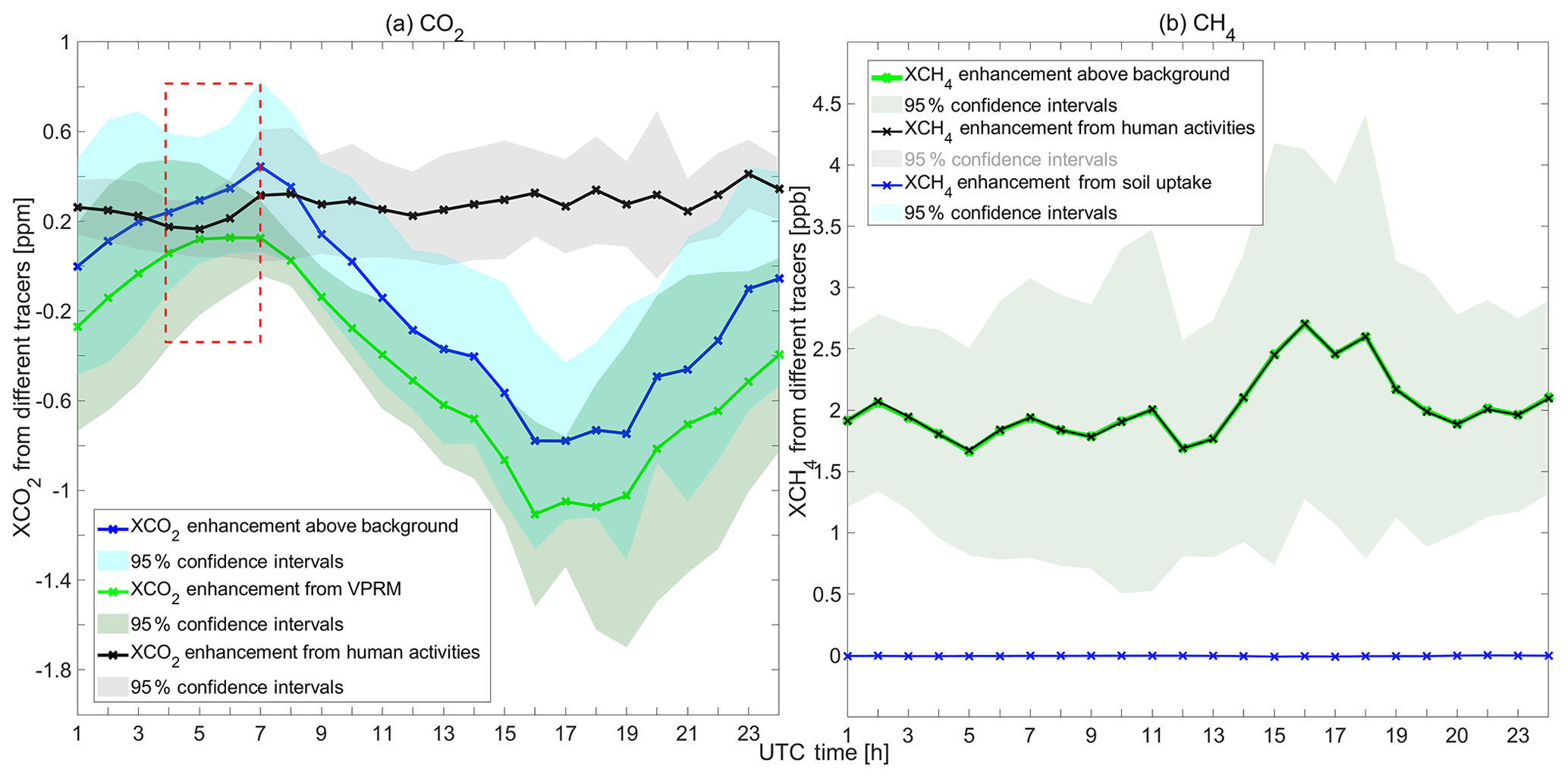
Figure 5The diurnal variations in the simulated changes in concentrations caused by different emission tracers in Charlottenburg in Berlin from 2014, averaged over a period of 9 d (from 2 to 10 July 2014). The colored lines represent the concentration changes and the mean enhancement over background. (a) The mean hourly XCO2,VPRM (green line) and XCO2,anthro (black line). (b) The mean hourly XCH4,anthro (black line) and XCH4,soil (blue line). The red box in (a) marks the morning peak of the XCO2 enhancement over the background, as described in Sect. 3.4.
As an instructive example of an analysis involving these tracers, we look at the diurnal cycle of contributions from the different tracers mentioned above in Charlottenburg (Fig. 5). The mean values, averaged over 9 d (from 2 to 10 July), as well as a 95 % confidential interval calculated in the averaging process are shown in Fig. 5. Figure 5a clearly shows a decline during the day and a rise at night in the XCO2 enhancement over the background (blue: XCO2,total – XCO2,bgd), with a maximum decrease over the course of the day of around 2 ppm. The XCO2 enhancement over the background reaches its daily peak during morning rush hour (07:00 UTC). The morning peak corresponds to XCO2 changes from human activities, depicted by the black line from 04:00 to 07:00 UTC (marked by a red square in Fig. 5a). Before the evening rush hour (16:00 UTC), XCO2 over the background then decreases, owning to biogenic uptake. Beginning in the evening, values increase again. The fluctuation in the evening (17:00–19:00 UTC) is dominated by XCO2 enhancements from human activities, while the substantial rise from 19:00 UTC onward is generated by the VPRM tracer, specifically the accumulation of the vegetation respiration in the evening.
XCO2 is weaker compared to the strong biogenic uptake. To further highlight the role of anthropogenic activities in XCO2 changes within the urban area, DCM is applied in Sect. 4. More specifically, we will use downwind-minus-upwind column differences of CO2 (ΔXCO2) to describe the XCO2 enhancement over an upwind site, as the difference between the downwind and upwind sites can be attributed to urban emissions.
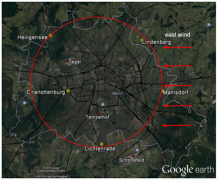
Figure 6Detailed locations of the five sampling sites. The five red stars stand for the five sampling sites, four of which (Mahlsdorf, Heiligensee, Lindenberg and Lichtenrade) were roughly situated along a circle with a radius of 12 km around the center of Berlin, marked as the black circle. The innermost domain of our WRF-GHG model contains all five measurement sites. The three wind measurement sites are marked by red circles. Map provided by © Google Earth, © GeoBasis DE/BKG and © Europa Technologies.
Turning to XCH4 in Fig. 5b, we plot the variations in the mean hourly contributions from the anthropogenic (black line: XCH4,anthro) and soil uptake tracer (blue line: XCH4,soil) in Charlottenburg. The contributions by anthropogenic activities fluctuate slightly around 2 ppb in the morning and at noon; then a peak occurs at the start of the evening rush hour (16:00 UTC). After 18:00 UTC, values clearly decrease, reaching approximately 2 ppb. From 21:00 UTC, XCH4 stabilizes, exhibiting only moderate fluctuations. The XCH4 enhancement above the background (green: ) depends largely on the XCH4 contributions by human activities. The changes in concentrations caused by the soil uptake tracer (blue), whose values fluctuate between 0.001 and 0.01 ppb, have almost no influence on the variation in the XCH4 enhancement over the background in the urban area.
4.1 Comparison of differential column concentrations
The DCM can be employed to detect and estimate local emission sources within an area, based on calculated concentration differences between downwind and upwind sites (Chen et al., 2016). The difference (ΔXG) of a specific gas G in column-averaged DMFs across the downwind and upwind sites is defined as
where XGdownwind and XGupwind represent the column-average DMFs at the downwind and upwind sites.
In this study, DCM is applied to measurements and models in the spirit of a post-processing analysis. This approach is not only useful for canceling out the bias of the simulated XCH4 (see Sect. 3.3) but also for assessing the role of anthropogenic activities in XCO2 changes more appropriately.
A necessary prerequisite for DCM is distinguishing the upwind and downwind sites among all five sampling sites. Wind direction thus plays a pivotal role in the calculation of the downwind-minus-upwind column differences. In this study, the hourly simulated vertically averaged wind directions are assumed as a standard to classify the sites into downwind and upwind sites. The tracer transport calculations in the first few hours are not stable in WRF-GHG. Thus, we select 3, 4, 6 and 10 July as our targeted dates.
Table 1The selections of upwind and downwind sites for four dates
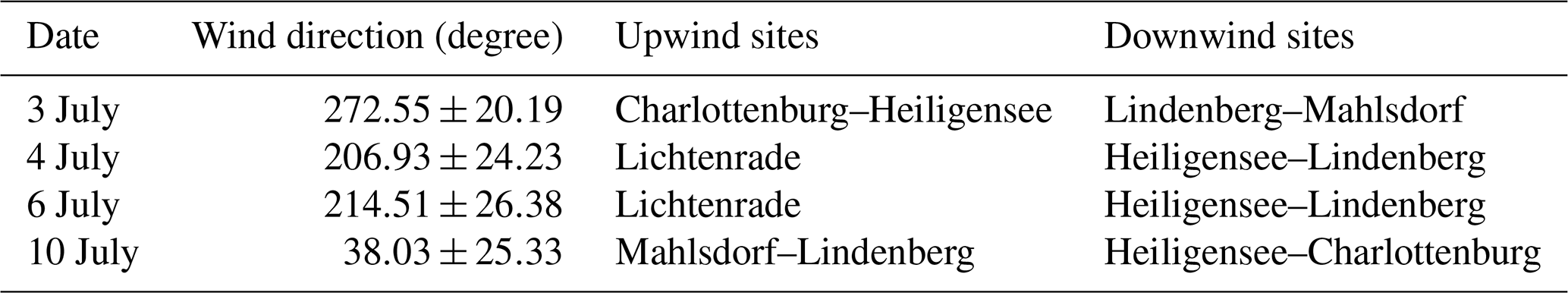
Wind directions are the mean of the hourly vertically averaged wind directions for 1 d.

Figure 7Modeled wind fields for downwind (blue lines) and upwind (red lines) sites (a–d), and downwind-minus-upwind differential evaluation for measured (blue) and simulated (black lines) XCH4 (e–h) on 3, 4, 6 and 10 July 2014. Based on the selection of downwind and upwind sites in Table 1, ΔXCH4 is calculated using Eqs. (6), (7) and (8), depicted by blue lines for measurements and black lines for simulations. The black error bars in (e–h) are the standard derivations of the minute values of the hourly mean.
Table 1 shows the daily averaged wind directions with standard derivations and the details on the downwind and upwind sites for these four target dates. West wind is the prevailing wind direction on 3 July. That is to say, Mahlsdorf and Lindenberg are downwind sites, and the upwind sites corresponding to these are Charlottenburg and Heiligensee, described in Eq. (6). The wind on 10 July is northeasterly, and the combination of downwind and upwind sites are selected to be opposite of the ones on 3 July, see Eq. (8). The prevailing winds on 4 and 6 July are easterly. The upwind site is Lichtenrade, and the corresponding downwind sites are Heiligensee and Lindenberg, see Eq. (7). Based on the selection of downwind and upwind sites shown in Table 1 and Eq. (5), differential column concentrations (ΔXCH4) are, therefore, calculated as
Figure 7 depicts the variations in the wind fields (wind speeds and wind directions) and ΔXCH4 (corresponding to Eqs. 6, 7 and 8) on 3, 4, 6 and 10 July. As depicted in the Fig. 7a–d, the hourly vertically averaged simulated wind speeds and directions at downwind and upwind sites are homogeneous. Thus, it is reasonable to use the daily mean wind directions as the standard for the selection of downwind and upwind sites. The general trends in the simulated ΔXCH4 values, shown in Fig. 7e–h, seem to be roughly reproduced by the observations but slightly overestimated, with an RMSE of 1.3895 ppb.
Yet DCM as presented here has the potential to highlight the role of anthropogenic activities, which we demonstrate, applying it to CO2 tracers in the simulation. Thus, the analysis on anthropogenic and biogenic tracers for CO2 will be especially prominent here. As described above, we continue to take 3, 4, 6 and 10 July as examples (see Fig. 8a–d).
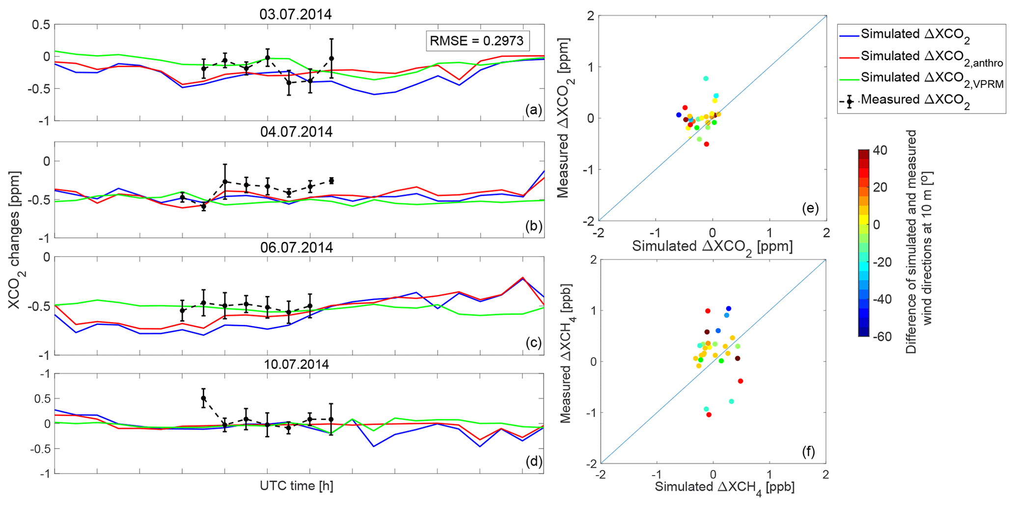
Figure 8Measured (black lines) and simulated (blue lines) ΔXCO2 on 3, 4, 6 and 10 July 2014, and comparison of hourly mean ΔXCO2 and ΔXCH4 for these 4 d. The ΔXCO2, calculated using Eqs. (6), (7) and (8), are depicted by blue lines in (a–d). The red and green lines show the variation in the differences between downwind and upwind sites in XCO2 changes from anthropogenic and biogenic activities, respectively. The points in (e–f) are coded by the difference of the simulated and measured wind directions at 10 m. The black error bars in (a–d) are the standard derivations of the minute values of the hourly mean.
The variations in ΔXCO2 (corresponding to Eqs. 6, 7 and 8) on 3, 4, 6 and 10 July are shown. In contrast to the variations in XCO2 values (Sect. 3.4; Fig. 5a), the simulated ΔXCO2 (Fig. 8a–d, blue lines) is not so much influenced by the XCO2 changes from the VPRM tracer (Fig. 8a–d, green) but more closely follows the XCO2 changes from anthropogenic activities (Fig. 8a–d, red). With DCM, the role of human activities in XCO2 changes is highlighted, and the strong effect from the biogenic component is canceled out. The ΔXCO2 measurements (Fig. 8a–d, black) show similar trends as the simulation with an RMSE of 0.2973 ppm.
To further understand the differences of ΔXCO2 and ΔXCH4 between measurements and simulations (see Fig. 7e–h and Fig. 8a–d), the comparison of hourly mean ΔXCO2 and ΔXCH4 values for these four targeted dates is illustrated in the right column of Fig. 8. Due to the restriction of measured wind information, we illustrate the differences of simulated and measured wind directions at 10 m (i.e., Fig. 2b) with respect to the hourly mean ΔXCO2 and ΔXCH4. We find that the real hourly mean ΔXCO2 and ΔXCH4 values are generally higher than the simulated values. Extreme points are colored by red and blue in the right column of Fig. 8e–f, standing for large differences between measured and simulated wind directions at 10 m. We see that a large difference of wind directions is a necessary but insufficient condition for the bias of ΔXCO2 and ΔXCH4 between measurements and simulations. In future studies, this is suggested as something to be verified further.
We conclude that DCM, as applied in this plot, reduces the model bias caused by the simulation initialization but introduces unpleasant effects which may be attributed to errors in the assumed or simulated wind directions.
4.2 Comparison between differential column concentrations and modeling results after the elimination of wind influence
As described in Sect. 4.1, the wind direction impacts the distinction between downwind and upwind sites for DCM. Devising meaningful and accurate recipes for determining the wind directions is not easy, sometimes resulting in mixed-quality results (of Sect. 4.1). Our simulated output provides the hourly wind and concentration fields. The instruments measure the concentration value every minute (Hase et al., 2015). We simply assume the wind direction to be a constant value within 1 h (the hourly vertically averaged values) in our calculation also when it comes to selecting upwind and downwind sites. This may create inaccuracies in the calculation of the measured ΔXCH4.
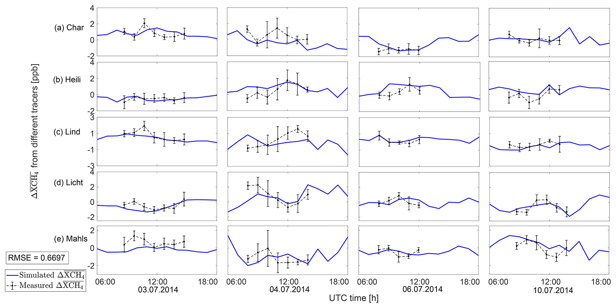
Figure 9Modeled (blue lines) and observed (black lines) site XCH4 vs. site-mean XCH4 data for five sampling sites: Charlottenburg (a: Char), Heiligensee (b: Heili), Lindenberg (c: Lind), Lichtenrade (d: Licht) and Mahlsdorf (e: Mahls). The black error bars in each subplot are the standard derivations of the minute values of the hourly mean.
In this section, we test replacing the upwind values in DCM by an all-site mean to provide a potential solution for the elimination of such problems while still applying the DCM. The mean of the column-averaged DMFs over all sampling sites () is assumed to be the background concentration within the entire urban region, replacing the XCH4 at the upwind site. The differences between the specific site and the mean of all the sites for each gas G () is then evaluated, i.e.,
where XGspecific site is the column-averaged DMF at the respective sampling site.
We now test this form of DCM for the same four targeted dates (3, 4, 6 and 10 July). The distance between any two sampling sites is around 25 km. The general trends of the simulated (Fig. 9, blue lines) and measured (Fig. 9, black lines) values appear to be more similar with an RMSE of 0.6698 ppb compared to the comparison of ΔXCH4 in Fig. 7e–h (RMSE of 1.3895 ppb). The model–measurement bias can be caused by underestimated emissions from anthropogenic activities, the smoothing of actual extreme values in the simulation and the ignorance of the line of the sun sight for the simulation. The variations in the XCH4 at the five different sampling sites on the same day are similar (Fig. 9), but the measurements show more extreme values (e.g., 4 July) compared to the simulations. A further analysis in a future study is suggested to provide deeper insight into site-specific transport characteristics.
As a final point in our analysis, we focus on simulated values for these four target dates (Fig. 10). The values (blue line) on 3, 4, 6 and 10 July in five sampling sites are mainly dominated by the XCO2 changes caused by the anthropogenic tracer (red) instead of the VPRM tracer (green). Compared to Fig. 8a–d, the red line and blue line in Fig. 10 show a stronger similarity in their trends. With this form of DCM (compared to the original form Eq. 5 in Sect. 4.1), anthropogenic activities can be clearly shown to influence XCO2 within urban areas. Meanwhile, the measurements (black lines) fit better with the simulation with an RMSE of 0.2333 ppm compared to the comparisons of ΔXCO2 depicted in Fig. 7a–d (RMSE of 0.2973 ppm).
We used WRF-GHG to quantitatively simulate the uptake, emission and transport of CO2 and CH4 for Berlin with a high resolution of 1 km. The simulated wind and concentration fields were compared with observations from 2014. Then, differential column methodology (DCM) was utilized as a post-processing method for the XCH4 comparison and the XCO2 tracer analysis.

Figure 10 (blue lines for simulations and black for measurements) for five sampling sites (i.e., the difference between XCO2 at the site and the mean XCO2 of five sampling sites): Charlottenburg (a: Char), Heiligensee (b: Heili), Lindenberg (c: Lind), Lichtenrade (d: Licht) and Mahlsdorf (e: Mahls). We furthermore show the differences in the simulated changes from biogenic (green lines) and anthropogenic (red lines) activities. The black error bars in each subplot are the standard derivations of the minute values of the hourly mean.
The measured and simulated wind fields at 10 m mostly demonstrate good agreement, but with slight errors in the wind directions. The simulated pressure vertical profile and the averaging kernel from the solar-viewing spectrometer (EM27/SUN) are used to obtain the smoothed pressure-weighted average concentration for further comparisons. The simulated XCO2 concentrations actually reproduce the observations well, but with approximately 1–2 ppm bias, which can be attributed to the coarse emission inventory, background concentrations from CAMS and the ignorance of the line of the sun sight for the simulation. Compared to the measured XCH4, some deviations can clearly be noted in the simulated XCH4, mostly caused by the relatively high background concentration fields and the errors at the tropopause height. We discussed the diurnal variation in concentration components corresponding to the major emission tracers for both CO2 and CH4. The biogenic component plays a pivotal role in the variations in XCO2. The impact from anthropogenic emission sources is somewhat weak compared to this, while the XCH4 enhancement is dominated by human activities.
We then concentrated on using DCM for focusing our analysis on relevant CO2 and CH4 contributions from the urban area. DCM highlights that the enhancement of XCO2 over the background within the inner Berlin urban area is mostly caused by anthropogenic activities. In DCM, wind direction plays a vital role in defining the upwind and downwind sites, which directly influence the calculation of differential column concentrations. In the CO2 tracer analysis, it turns out that , the difference with respect to a mean value instead of a specific upwind site, exhibits a more visible and clearer trend, which proves that the CO2 enhancement is dominated by anthropogenic activities within the urban area. We conclude that DCM, when applied with care, helps in highlighting the relevant emission sources. Similarly, for XCH4, DCM eliminates the bias of the simulated values. Furthermore, when ΔXCH4 values suffer from inconsistent wind directions, we consider to be a useful quantity for analysis.
An analysis of XCO2 in the Paris hotspot region was carried out by Vogel et al. (2019). Some of their results can be compared to the conclusions we drew in this paper. In Vogel et al. (2019), the modeled XCO2 was calculated based on the chemistry transport model CHIMERE (2 km) and flux framework CAMS (15 km), with hourly anthropogenic emissions from the IER (Institut für Energiewirtschaft und Rationelle Energieanwendung; University of Stuttgart, Germany) and EDGAR emission inventories and the natural fluxes prescribed by the CTESSEL model (Sect. 2 in Vogel et al., 2019). When comparing results from our simulation, the diurnal variation in the XCO2 enhancement over the background (Sect. 3.4 and Fig. 5a of our paper) is comparable to the findings of Vogel et al. (2019). For the analysis on the comparison of ΔXCH4 between simulations and measurements in Sect. 4.1, we found that negative column concentration differences between downwind and upwind sites appear for some periods, owing to the variation in wind directions that causes the conversion of upwind and downwind sites, which was also mentioned for the ΔXCO2 analysis in Vogel et al. (2019). Based on the CHIMERE-CAMS modeling framework, they showed that the strong decrease in XCO2 during daytime can be linked to net ecosystem exchange, while a significant enhancement compared to the background is caused by XCO2 from fossil-fuel emissions, but this is often compensated by net ecosystem exchange. We utilized DCM to bring out the role of anthropogenic activities within urban areas (see the XCO2 tracer analysis in Sect. 4 of our paper).
We conclude that WRF-GHG is a suitable model for precise GHG transport analysis in urban areas, especially when combined with DCM. DCM is not only useful for the direct evaluation of measurements but also helps us to understand the results of tracer transport models, canceling out the bias caused by initialization conditions, for example, and highlighting regional emission sources. This case is a fundamental study for the WRF-GHG mesoscale modeling framework. Emission flux estimations using WRF-GHG would be our further target to be demonstrated for the case of Munich. This Munich case is combined with the first worldwide permanent column measurement network designed in Munich. Various emission tracers will be run for this case in which more emission tracers (e.g., biogenic emissions from wetland for XCH4, traffic emission and strong point source emissions in urban areas) are being separated and analyzed using the longer time period of available measurements.
In future work, we suggest running WRF-GHG for more urban areas such that, for example, different transport, more emission tracers, topography, emission scenarios and the quantification of model errors can be studied. The influence from the line of the sun sight should be taken into account, and the relative sensitivity analysis is suggested. The WRF-GHG mesoscale simulation framework may also be combined with microscale atmospheric transport models to simulate crucial details of emission sources and transport patterns precisely, with the aim of tracing urban GHG emissions. A further promising direction for future studies may be the application of DCM and model-based analysis to satellite measurements to assess gradients across column concentrations with a dense spatial sampling.
The simulation data that support the findings of this study are available on request from the corresponding author. The measurement data are available at https://doi.org/10.5194/amt-8-3059-2015 (Hase et al., 2015).
A detailed description on how to run WRF-GHG is provided in Beck et al. (2011), and thus, only the initialization process for our study in particular is summarized here. One daily simulation with WRF-GHG is normally performed for a 30 h time period, including a 6 h spin-up for the meteorology from 18:00 to 24:00 UTC of the previous day and a 24 h simulation of the tracer transport on the actual simulation day (Beck et al., 2011).
As for the boundary conditions, a small constant offset needs to be added into the WRF boundary files for the biospheric CO2 and the soil sink CH4 tracers at the start of each run because these tracers can result in a net sink. When the concentrations become negative, the advected tracer fields will “disappear”, as the WRF code does not allow tracers with negative values. An offset applied in the initialization process helps to avoid this problem and later is subtracted in the post-processing. As for the initial conditions, the meteorological conditions are initialized with external data sources (GFS in our model) each day to update the WRF meteorological fields properly. The tracers for the total and background CO2 and CH4 flux fields are initialized only once, at the first day of the simulation period, using CAMS as an external data source. Furthermore, the lateral boundary conditions of the outer domain d01 are also initialized by the CAMS. Then, for the other days within the simulation period, these tracers for the total and background CO2 and CH4 fluxes are directly taken from the final WRF output at 24:00 UTC of the previous day to make the entire simulation continuous. The CO2 tracer for VPRM and the CH4 tracer for soil uptake are also initialized with a constant offset to avoid the appearance of negative values caused, for example, by the vegetation respiration (Beck et al., 2011). In terms of the other flux tracers, the tracer variables are initialized each day, using external data sources to provide the updated emission data for each tracer.
In the passive tracer transport simulation, the total concentration of each GHG is represented as a separate tracer, giving redundant information (with respect to the sum of all tracers for each GHG) and allowing for consistency checks. A variety of flux models and emission inventories implemented in the modules of WRF-GHG are used for the estimation of GHG fluxes. The flux values from external emission inventories are gridded and absorbed into the model. In the transport process, the relationship among the changes in concentrations from different emission tracers, the total and background concentrations (Eq. 1) should then be satisfied, ideally with ΔCO2 and ΔCH4 computational errors during the simulation process being zero. Nonzero values of ΔCO2 and ΔCH4 reflect the limited precision of the tracer transport calculation in WRF-GHG.

Figure B1The mean values (solid lines) and the 95 % confidence intervals of the computational error ΔCO2 (a) and ΔCH4 (b). ΔCO2 and ΔCH4 are calculated using Eq. (1).
Figure B1 thus shows the mean values (solid lines) and the 95 % confidence intervals of ΔCO2 and ΔCH4. As depicted in the figure, ΔCO2 ranges from −0.005 to 0.01 ppm, while ΔCH4 is in the range of −0.01 to 0.02 ppb. Divided by typical absolute values of the concentrations from different flux processes for XCO2 (around 1 ppm) and XCH4 (around 2–3 ppb) depicted in Fig. 4, the relative computational error is found to be ∼ 1 % for both CO2 and CH4.
These tiny computational errors can be caused by the slight non-linearity of the advection scheme used in the WRF-GHG model, which makes the sum of the concentrations in CO2 and CH4 from all individual flux tracers not exactly equal to the concentration from the sum tracer, representing the total sum of all fluxes related to different processes.
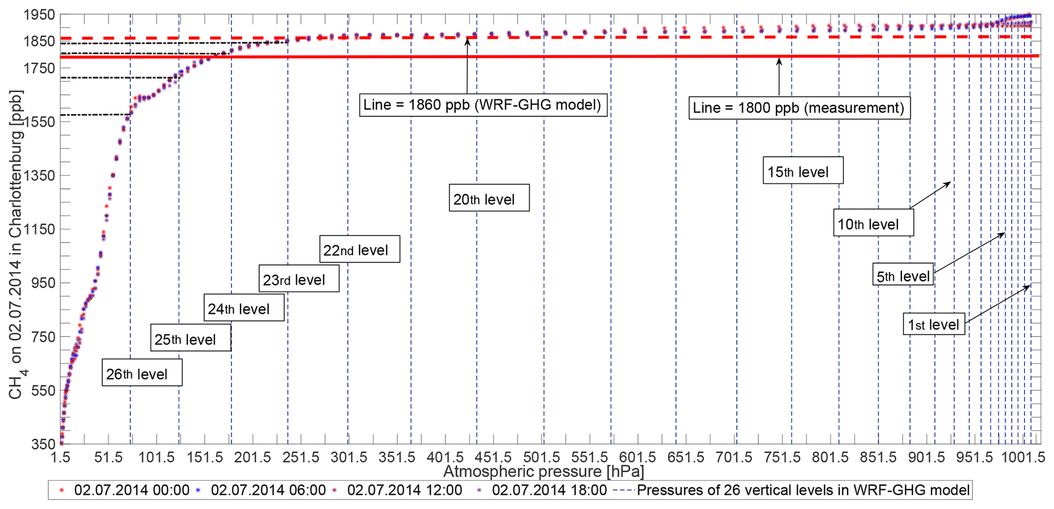
Figure C1The vertical distribution of CH4 on 2 July in Charlottenburg. The asterisks represent the XCH4 field from CAMS. The vertical dashed lines show the values of atmospheric pressure corresponding to the 26 vertical levels in our WRF-GHG. y axis levels of 1800 and 1860 ppb, corresponding to the total column measurement and the modeled value, respectively, have been marked by red horizontal (solid and dashed) lines.

Figure D1Comparison of XCO2 from WRF-GHG with and without smoothing (using our column sensitivities for EM27/SUN) for the first four simulated dates. The five colors stand for the concentrations from five sample sites. Dotted lines with the crosses represent the XCO2 without smoothing, while solid lines with the circles stand for the smoothed values.
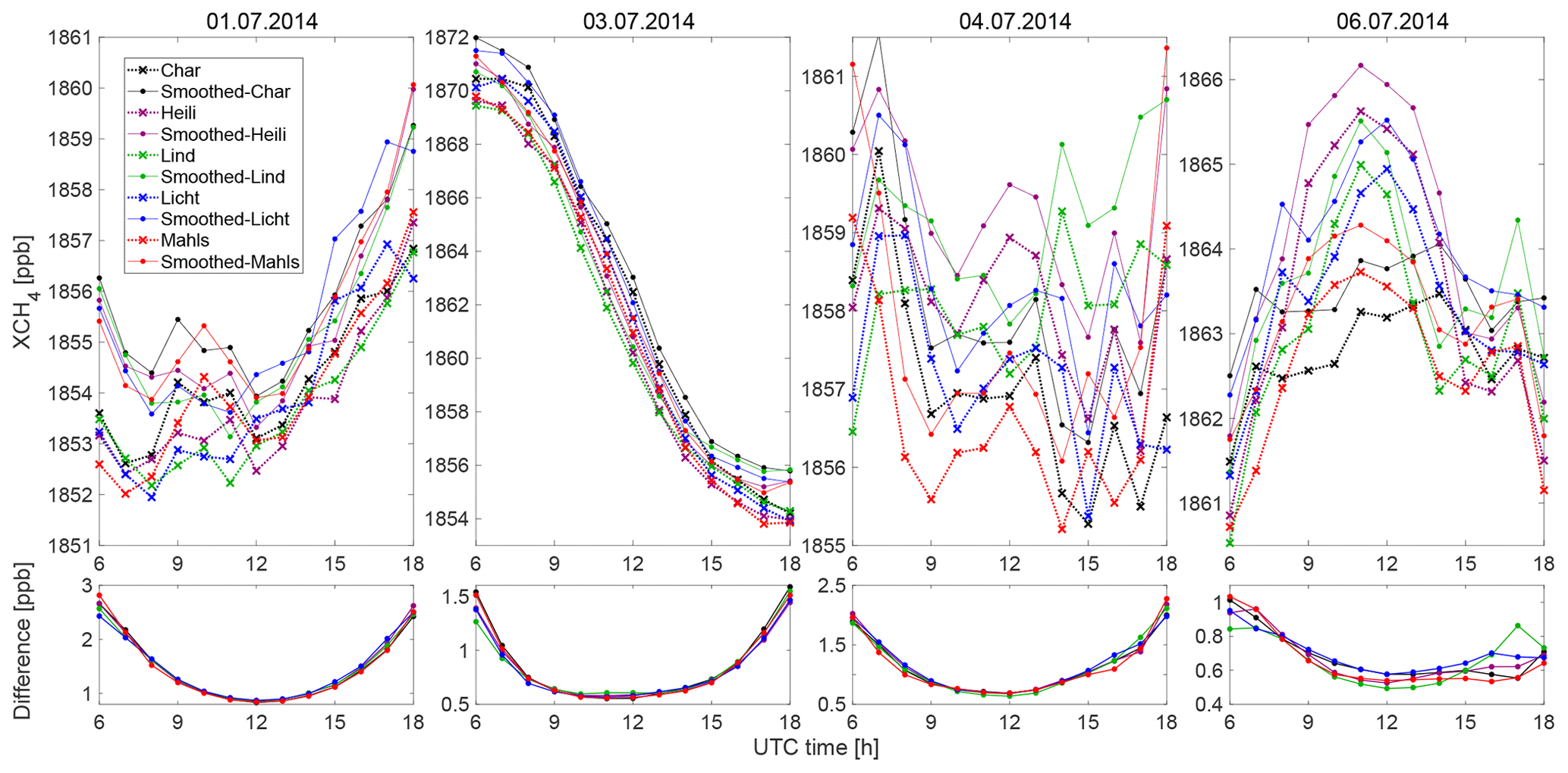
Figure D2Comparison of XCH4 from WRF-GHG with and without smoothing (using our column sensitivities for EM27/SUN) for the first four simulated dates. The five colors stand for the concentrations from five sample sites. Dotted lines with the crosses represent the XCH4 without smoothing, while solid lines with the circles stand for the smoothed values.
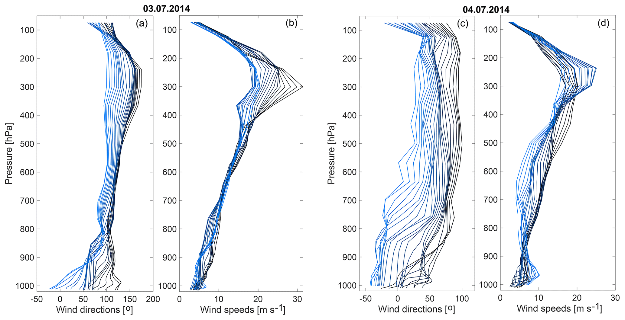
Figure E1The vertical distribution of wind fields (wind speeds and wind directions) on 3 July (a, b) and 4 July (c, d) in Tegel. The colors from black to blue represent the time from morning to evening.
XZ performed the simulations, with the support and guidance of JM, CG, JC and SH. JM provided the CAMS fields for the initialization. JC supplied the anthropogenic emission source, and CG offered the VPRM used for the simulations. MF and FH provided the measurement data for Berlin in 2014 and fruitful discussions related to the measurements. SH provided the guidance related to the running of the simulations in the Linux cluster. XZ, JC and SH designed the computational framework. XZ and JC performed the analysis of the results. XZ wrote the paper, with input from all authors. All authors provided critical feedback and helped shape the research, analysis and paper.
The authors declare that they have no conflict of interest.
We thank the personal contribution from Michal Galkowski from the Max Planck Institute for Biogeochemistry for the biogenically related CH4 flux estimates. The a priori concentration profiles from the Whole Atmosphere Community Climate Model (WACCM) were provided by James W. Hannigan (NCAR). Jia Chen is partly supported by the Technical University of Munich Institute for Advanced Study, funded by the German Excellence Initiative and the European Union Seventh Framework Programme under grant agreement no. 291763. The simulations presented in this work have been run on the Linux cluster (CooLMUC-2) of the Leibniz Supercomputing Centre (LRZ; Garching). We acknowledge support by the ACROSS research infrastructure of the Helmholtz Association.
The article processing charges for this open-access publication were covered by the Max Planck Society.
This paper was edited by Stefano Galmarini and reviewed by two anonymous referees.
Agusti-Panareda, A., Diamantakis, M., Bayona, V., Klappenbach, F., and Butz, A.: Improving the inter-hemispheric gradient of total column atmospheric CO2 and CH4 in simulations with the ECMWF semi-Lagrangian atmospheric global model, Geosci. Model Dev., 10, 1–18, https://doi.org/10.5194/gmd-10-1-2017, 2017. a
Ahmadov, R., Gerbig, C., Kretschmer, R., Koerner, S., Neininger, B., Dolman, A., and Sarrat, C.: Mesoscale covariance of transport and CO2 fluxes: Evidence from observations and simulations using the WRF-VPRM coupled atmosphere-biosphere model, J. Geophys. Res.-Atmos., 112, D22107, https://doi.org/10.1029/2007JD008552, 2007. a, b
Ahmadov, R., Gerbig, C., Kretschmer, R., Körner, S., Rödenbeck, C., Bousquet, P., and Ramonet, M.: Comparing high resolution WRF-VPRM simulations and two global CO2 transport models with coastal tower measurements of CO2, Biogeosciences, 6, 807–817, https://doi.org/10.5194/bg-6-807-2009, 2009. a
Andres, R. J., Boden, T. A., Bréon, F.-M., Ciais, P., Davis, S., Erickson, D., Gregg, J. S., Jacobson, A., Marland, G., Miller, J., Oda, T., Olivier, J. G. J., Raupach, M. R., Rayner, P., and Treanton, K.: A synthesis of carbon dioxide emissions from fossil-fuel combustion, Biogeosciences, 9, 1845–1871, https://doi.org/10.5194/bg-9-1845-2012, 2012. a
Basart, S., Bendictow, A., Blechschmidt, A.-M., Chabrillat, S., Clark, H., Cuevas, E., Flentje, H., Hansen, K. M., Kapsomenakis, U. Im, J., Langerock, B., Petersen, K., Richter, A., Sudarchikova, N., Thouret, V., Warneke, T., and Zerefos, C.: Validation report of the CAMS near-real time global atmospheric composition service, Copernicus Atmosphere Monitoring Service (CAMS), available at: https://atmosphere.copernicus.eu/sites/default/files/repository/CAMS84_2015SC2_D84.1.1.7_2017DJF_v1.1_0.pdf (last access: 22 July 2019), 2017. a
Beck, V., Koch, T., Kretschmer, R., Marshall, J., Ahmadov, R., Gerbig, C., Pillai, D., and Heimann, M.: The WRF Greenhouse Gas Model (WRF-GHG). Technical Report No. 25, Max Planck Institute for Biogeochemistry, Jena, Germany, 2011. a, b, c, d, e, f, g
Bergamaschi, P., Corazza, M., Karstens, U., Athanassiadou, M., Thompson, R. L., Pison, I., Manning, A. J., Bousquet, P., Segers, A., Vermeulen, A. T., Janssens-Maenhout, G., Schmidt, M., Ramonet, M., Meinhardt, F., Aalto, T., Haszpra, L., Moncrieff, J., Popa, M. E., Lowry, D., Steinbacher, M., Jordan, A., O'Doherty, S., Piacentino, S., and Dlugokencky, E.: Top-down estimates of European CH4 and N2O emissions based on four different inverse models, Atmos. Chem. Phys., 15, 715–736, https://doi.org/10.5194/acp-15-715-2015, 2015. a
Bergamaschi, P., Karstens, U., Manning, A. J., Saunois, M., Tsuruta, A., Berchet, A., Vermeulen, A. T., Arnold, T., Janssens-Maenhout, G., Hammer, S., Levin, I., Schmidt, M., Ramonet, M., Lopez, M., Lavric, J., Aalto, T., Chen, H., Feist, D. G., Gerbig, C., Haszpra, L., Hermansen, O., Manca, G., Moncrieff, J., Meinhardt, F., Necki, J., Galkowski, M., O'Doherty, S., Paramonova, N., Scheeren, H. A., Steinbacher, M., and Dlugokencky, E.: Inverse modelling of European CH4 emissions during 2006–2012 using different inverse models and reassessed atmospheric observations, Atmos. Chem. Phys., 18, 901–920, https://doi.org/10.5194/acp-18-901-2018, 2018. a
Caulton, D. R., Shepson, P. B., Santoro, R. L., Sparks, J. P., Howarth, R. W., Ingraffea, A. R., Cambaliza, M. O., Sweeney, C., Karion, A., Davis, K. J., Stirm, B. H., Montzka, S. A., and Miller, B. R.: Toward a better understanding and quantification of methane emissions from shale gas development, P. Natl. Acad. Sci. USA, 111, 6237–6242, https://doi.org/10.1073/pnas.1316546111, 2014. a
Chen, F., Kusaka, H., Bornstein, R., Ching, J., Grimmond, C., Grossman-Clarke, S., Loridan, T., Manning, K. W., Martilli, A., Miao, S., Sailor, D., Salamanca, F. P., Taha, H., Tewari, M., Wang, X., Wyszogrodzki, A. A., and Zhang, C.: The integrated WRF/urban modelling system: development, evaluation, and applications to urban environmental problems, Int. J. Climatol., 31, 273–288, https://doi.org/10.1002/joc.2158, 2011. a
Chen, J., Samra, J., Gottlieb, E., Budney, J., Daube, C., Daube, B. C., Hase, F., Gerbig, C., Chance, K., and Wofsy, S. C.: Boston Column Network: Compact Solar-Tracking Spectrometers and Differential Column Measurements, AGU Fall meeting, San Francisco, USA, 15–19 December 2014, A53L-3381, 2014. a
Chen, J., Viatte, C., Hedelius, J. K., Jones, T., Franklin, J. E., Parker, H., Gottlieb, E. W., Wennberg, P. O., Dubey, M. K., and Wofsy, S. C.: Differential column measurements using compact solar-tracking spectrometers, Atmos. Chem. Phys., 16, 8479–8498, https://doi.org/10.5194/acp-16-8479-2016, 2016. a, b, c
Chen, J., Dietrich, F., Franklin, J. E., Jones, T. S., André, B., Luther, A., Kleinschek, R., Hase, F., Wenig, M., Ye, S., Nouri, A., Frey, M., Knote, C., Alberti, C., and Wofsy, S.: Mesoscale column network for assessing GHG and NOx emissions in Munich, EGU General Assembly Conference Abstracts, Vol. 20, EGU2018-10192-2, Vienna, Austria, 8–13 April 2018, 2018. a
Cressot, C., Chevallier, F., Bousquet, P., Crevoisier, C., Dlugokencky, E. J., Fortems-Cheiney, A., Frankenberg, C., Parker, R., Pison, I., Scheepmaker, R. A., Montzka, S. A., Krummel, P. B., Steele, L. P., and Langenfelds, R. L.: On the consistency between global and regional methane emissions inferred from SCIAMACHY, TANSO-FTS, IASI and surface measurements, Atmos. Chem. Phys., 14, 577–592, https://doi.org/10.5194/acp-14-577-2014, 2014. a
Deutscher, N. M., Notholt, J., Messerschmidt, J., Weinzierl, C., Warneke, T., Petri, C., Grupe, P., and Katrynski, K.: TCCON data from Bialystok (PL), Release GGG2014R1, TCCON data archive, hosted by CaltechDATA, https://doi.org/10.14291/tccon.ggg2014.bialystok01.R1/1183984, 2014. a
Fragkias, M., Lobo, J., Strumsky, D., and Seto, K. C.: Does size matter? Scaling of CO2 emissions and US urban areas, PLoS One, 8, e64727, https://doi.org/10.1371/journal.pone.0064727, 2013. a
Franklin, J. E., Jones, T. S., Chen, J., Parker, H., Hedelius, J., Wennberg, P., Dubey, M. K., Cohen, Ron C., G. A., Sargent, M., Davis, K. J., Mielke, L., Fischer, M., and Wofsy, S.: A three-dimensional observation network for determining urban emissions of CO2 and CH4, 2017 North American Carbon Program, North Bethesda, MD, USA, available at: https://www.nacarbon.org/meeting_2017/abs_and_discussions/mtg2017_ab_searchab_id161.html (last access: 22 July 2019), 2017. a
Fraunhofer-Gesellschaft: ISE: Map of Power Plants, Energy Chart, data source: European Energy Exchange (EEX), available at: https://www.energy-charts.de/osm.htm, last access: 14 August 2018. a
Frey, M., Hase, F., Blumenstock, T., Groß, J., Kiel, M., Mengistu Tsidu, G., Schäfer, K., Sha, M. K., and Orphal, J.: Calibration and instrumental line shape characterization of a set of portable FTIR spectrometers for detecting greenhouse gas emissions, Atmos. Meas. Tech., 8, 3047–3057, https://doi.org/10.5194/amt-8-3047-2015, 2015. a, b, c
Friedl, M. A., Sulla-Menashe, D., Tan, B., Schneider, A., Ramankutty, N., Sibley, A., and Huang, X.: MODIS collection 5 global land cover: Algorithm refinements and characterization of new datasets, 2001–2012, Collection 5.1 IGBP Land Cover, Boston University, Boston, MA, USA, 2010. a
Galkowski, M., Gerbig, C., Marshall, J., Koch, F., Chen, J., Baum, S., Jordan, M., Fiehn, A., Roiger, A., Jöckel, P., Nickl, A., Mertens, M., Bovensmann, H., Necki, J., Swolkien, J., Ehret, G., Kiemle, C., Amediek, A., Quatrevalet, M., and Fix, A.: Airborne in-situ measurements of CO2 and CH4 and their interpretation using WRF-GHG: results from the HALO CoMet 1.0 campaign, EGU General Assembly Conference Abstracts, Vol. 21, EGU2019-14091, Vienna, Austria, 8–13 April 2019, 2019. a
Gerbig, C., Körner, S., and Lin, J. C.: Vertical mixing in atmospheric tracer transport models: error characterization and propagation, Atmos. Chem. Phys., 8, 591–602, https://doi.org/10.5194/acp-8-591-2008, 2008. a
Gisi, M., Hase, F., Dohe, S., Blumenstock, T., Simon, A., and Keens, A.: XCO2-measurements with a tabletop FTS using solar absorption spectroscopy, Atmos. Meas. Tech., 5, 2969–2980, https://doi.org/10.5194/amt-5-2969-2012, 2012. a
Hardiman, B. S., Wang, J. A., Hutyra, L. R., Gately, C. K., Getson, J. M., and Friedl, M. A.: Accounting for urban biogenic fluxes in regional carbon budgets, Sci. Total Environ., 592, 366–372, https://doi.org/10.1016/j.scitotenv.2017.03.028, 2017. a
Hase, F., Frey, M., Blumenstock, T., Groß, J., Kiel, M., Kohlhepp, R., Mengistu Tsidu, G., Schäfer, K., Sha, M. K., and Orphal, J.: Application of portable FTIR spectrometers for detecting greenhouse gas emissions of the major city Berlin, Atmos. Meas. Tech., 8, 3059–3068, https://doi.org/10.5194/amt-8-3059-2015, 2015. a, b, c, d, e, f, g, h, i, j, k
Hedelius, J. K., Viatte, C., Wunch, D., Roehl, C. M., Toon, G. C., Chen, J., Jones, T., Wofsy, S. C., Franklin, J. E., Parker, H., Dubey, M. K., and Wennberg, P. O.: Assessment of errors and biases in retrievals of , XCH4, XCO, and from a 0.5 cm−1 resolution solar-viewing spectrometer, Atmos. Meas. Tech., 9, 3527–3546, https://doi.org/10.5194/amt-9-3527-2016, 2016. a, b
Holmes, C. D.: Methane Feedback on Atmospheric Chemistry: Methods, Models, and Mechanisms, J. Adv. Model. Earth Sy., 10, 1087–1099, https://doi.org/10.1002/2017MS001196, 2018. a
Homann, G.: Climate Protection in Berlin, Tech. rep., Senate Department for the Environment, Transport and Climate Protection, available at: https://www.berlin.de/senuvk/klimaschutz/politik/download/klimaschutzpolitik_en.pdf (last access: 22 July 2019), 2018. a
Hopkins, F. M., Ehleringer, J. R., Bush, S. E., Duren, R. M., Miller, C. E., Lai, C.-T., Hsu, Y.-K., Carranza, V., and Randerson, J. T.: Mitigation of methane emissions in cities: How new measurements and partnerships can contribute to emissions reduction strategies, Earth's Future, 4, 408–425, https://doi.org/10.1002/2016EF000381, 2016. a, b
IEA (International Energy Agency): World Energy Outlook 2008, available at: https://www.iea.org/media/weowebsite/2008-1994/WEO2008.pdf (last access: 22 July 2019), 2008. a
IEA (International Energy Agency): Cities, Towns & Renewable Energy, Tech. rep., available at: http://www.iea.org/publications/freepublications/publication/cities2009.pdf (last access: 22 July 2019), 2009. a
IPCC (International Panel on Climate Change): IPCC fifth assessment report: Climate change 2014 Synthesis Report, Summary for Policymakers, available at: http://www.ipcc.ch/pdf/assessment-report/ar5/syr/AR5_SYR_FINAL_SPM.pdf (last access: 22 July 2019), 2014. a
Janssens-Maenhout, G., Crippa, M., Guizzardi, D., Dentener, F., Muntean, M., Pouliot, G., Keating, T., Zhang, Q., Kurokawa, J., Wankmüller, R., Denier van der Gon, H., Kuenen, J. J. P., Klimont, Z., Frost, G., Darras, S., Koffi, B., and Li, M.: HTAP_v2.2: a mosaic of regional and global emission grid maps for 2008 and 2010 to study hemispheric transport of air pollution, Atmos. Chem. Phys., 15, 11411–11432, https://doi.org/10.5194/acp-15-11411-2015, 2015. a
Kennedy, C., Steinberger, J., Gasson, B., Hansen, Y., Hillman, T., Havranek, M., Pataki, D., Phdungsilp, A., Ramaswami, A., and Mendez, G. V.: Greenhouse gas emissions from global cities, Environ. Sci. Technol., 43, 7297–7302, https://doi.org/10.1021/es900213p, 2009. a
Kindler, A., Klimeczek, H.-J., and Franck, U.: Socio-spatial distribution of airborne outdoor exposures – An indicator for environmental quality, quality of life, and environmental justice: The case study of Berlin, in: Urban Transformations, edited by: Kabisch, S., Koch, F., Gawel, E., Haase, A., Knapp, S., Krellenberg, K., Nivala, J., and Zehnsdorf, A., 257–279, Springer, https://doi.org/10.1007/978-3-319-59324-1_14, 2018. a
Kivi, R. and Heikkinen, P.: Fourier transform spectrometer measurements of column CO2 at Sodankylä, Finland, Geosci. Instrum. Method. Data Syst., 5, 271–279, https://doi.org/10.5194/gi-5-271-2016, 2016. a, b
Kretschmer, R., Gerbig, C., Karstens, U., and Koch, F.-T.: Error characterization of CO2 vertical mixing in the atmospheric transport model WRF-VPRM, Atmos. Chem. Phys., 12, 2441–2458, https://doi.org/10.5194/acp-12-2441-2012, 2012. a
Mahadevan, P., Wofsy, S. C., Matross, D. M., Xiao, X., Dunn, A. L., Lin, J. C., Gerbig, C., Munger, J. W., Chow, V. Y., and Gottlieb, E. W.: A satellite-based biosphere parameterization for net ecosystem CO2 exchange: Vegetation Photosynthesis and Respiration Model (VPRM), Global Biogeochem. Cy., 22, GB2005, https://doi.org/10.1029/2006GB002735, 2008. a
Marcotullio, P. J., Sarzynski, A., Albrecht, J., Schulz, N., and Garcia, J.: The geography of global urban greenhouse gas emissions: An exploratory analysis, Climatic Change, 121, 621–634, https://doi.org/10.1007/s10584-013-0977-z, 2013. a
McKain, K., Wofsy, S. C., Nehrkorn, T., Eluszkiewicz, J., Ehleringer, J. R., and Stephens, B. B.: Assessment of ground-based atmospheric observations for verification of greenhouse gas emissions from an urban region, P. Natl. Acad. Sci. USA, 109, 8423–8428, https://doi.org/10.1073/pnas.1116645109, 2012. a, b
Montzka, S. A., Dlugokencky, E. J., and Butler, J. H.: Non-CO2 greenhouse gases and climate change, Nature, 476, 43–50, https://doi.org/10.1038/nature10322, 2011. a, b
Muntean, M., Janssens-Maenhout, G., Song, S., Selin, N. E., Olivier, J. G., Guizzardi, D., Maas, R., and Dentener, F.: Trend analysis from 1970 to 2008 and model evaluation of EDGAR.V4 global gridded anthropogenic mercury emissions, Sci. Total Environ., 494, 337–350, https://doi.org/10.1016/j.scitotenv.2014.06.014, 2014. a
Newman, S., Xu, X., Gurney, K. R., Hsu, Y. K., Li, K. F., Jiang, X., Keeling, R., Feng, S., O'Keefe, D., Patarasuk, R., Wong, K. W., Rao, P., Fischer, M. L., and Yung, Y. L.: Toward consistency between trends in bottom-up CO2 emissions and top-down atmospheric measurements in the Los Angeles megacity, Atmos. Chem. Phys., 16, 3843–3863, https://doi.org/10.5194/acp-16-3843-2016, 2016. a
Notholt, J., Petri, C., Warneke, T., Deutscher, N. M., Buschmann, M., Weinzierl, C., Macatangay, R., and Grupe, P.: TCCON data from Bremen (DE), Release GGG2014R0, TCCON data archive, hosted by CaltechDATA, https://doi.org/10.14291/tccon.ggg2014.bremen01.R0/1149275, 2014. a
Ohyama, H., Morino, I., Nagahama, T., Machida, T., Suto, H., Oguma, H., Sawa, Y., Matsueda, H., Sugimoto, N., Nakane, H., and Nakagawa, K.: Column-averaged volume mixing ratio of CO2 measured with ground-based Fourier transform spectrometer at Tsukuba, J. Geophys. Res.-Atmos., 114, D18303, https://doi.org/10.1029/2008JD011465, 2009. a
Olsen, S. C. and Randerson, J. T.: Differences between surface and column atmospheric CO2 and implications for carbon cycle research, J. Geophys. Res.-Atmos., 109, D02301, https://doi.org/10.1029/2003JD003968, 2004. a
Ostler, A., Sussmann, R., Patra, P. K., Houweling, S., De Bruine, M., Stiller, G. P., Haenel, F. J., Plieninger, J., Bousquet, P., Yin, Y., Saunois, M., Walker, K. A., Deutscher, N. M., Griffith, D. W. T., Blumenstock, T., Hase, F., Warneke, T., Wang, Z., Kivi, R., and Robinson, J.: Evaluation of column-averaged methane in models and TCCON with a focus on the stratosphere, Atmos. Meas. Tech., 9, 4843–4859, https://doi.org/10.5194/amt-9-4843-2016, 2016. a
Parshall, L., Gurney, K., Hammer, S. A., Mendoza, D., Zhou, Y., and Geethakumar, S.: Modeling energy consumption and CO2 emissions at the urban scale: Methodological challenges and insights from the United States, Energ. Policy, 38, 4765–4782, https://doi.org/10.1016/j.enpol.2009.07.006, 2010. a
Pillai, D., Gerbig, C., Ahmadov, R., Rödenbeck, C., Kretschmer, R., Koch, T., Thompson, R., Neininger, B., and Lavrié, J. V.: High-resolution simulations of atmospheric CO2 over complex terrain – representing the Ochsenkopf mountain tall tower, Atmos. Chem. Phys., 11, 7445–7464, https://doi.org/10.5194/acp-11-7445-2011, 2011. a, b, c
Pillai, D., Gerbig, C., Kretschmer, R., Beck, V., Karstens, U., Neininger, B., and Heimann, M.: Comparing Lagrangian and Eulerian models for CO2 transport – a step towards Bayesian inverse modeling using WRF/STILT-VPRM, Atmos. Chem. Phys., 12, 8979–8991, https://doi.org/10.5194/acp-12-8979-2012, 2012. a
Pillai, D., Buchwitz, M., Gerbig, C., Koch, T., Reuter, M., Bovensmann, H., Marshall, J., and Burrows, J. P.: Tracking city CO2 emissions from space using a high-resolution inverse modelling approach: a case study for Berlin, Germany, Atmos. Chem. Phys., 16, 9591–9610, https://doi.org/10.5194/acp-16-9591-2016, 2016. a, b
Reusswig, F., Hirschl, B., and Lass, W.: Climate-Neutrality Berlin 2050: Results of a Feasibility Study, Tech. rep., Senate Department for Urban Development and the Environment, available at: https://www.berlin.de/senuvk/klimaschutz/studie_klimaneutrales_berlin/download/Machbarkeitsstudie_Berlin2050_EN.pdf (last access: 22 July 2019), 2014. a
Rodgers, C. D. and Connor, B. J.: Intercomparison of remote sounding instruments, J. Geophys. Res.-Atmos., 108, 4116, https://doi.org/10.1029/2002JD002299, 2003. a
Saikawa, E., Kim, H., Zhong, M., Avramov, A., Zhao, Y., Janssens-Maenhout, G., Kurokawa, J.-I., Klimont, Z., Wagner, F., Naik, V., Horowitz, L. W., and Zhang, Q.: Comparison of emissions inventories of anthropogenic air pollutants and greenhouse gases in China, Atmos. Chem. Phys., 17, 6393–6421, https://doi.org/10.5194/acp-17-6393-2017, 2017. a
Sembhi, H., Boesch, H., Agusti-Panareda, A., and Massart, S.: MACC-III project (Monitoring AtmosphericComposition and Climate), available at: ftp://ftp.ecmwf.int/pub/macc/GHG/MACC_REPORTS/MACCIII_ULeicester_D42.3_Sembhi_final.pdf (last access: 22 July 2019), 2015. a
SenStadtH: Berlin Environmental Atlas: 06.01 Actual Use of Built-up Areas/06.02 Inventory of Green and Open Spaces/06.01.1 Actual Use/06.02.1 Actual Use and Vegetation Cover (Edition 2016), available at: http://www.stadtentwicklung.berlin.de/umwelt/umweltatlas/e_text/eke601.pdf (last access: 22 July 2019), 2016. a
Skamarock, W. C., Klemp, J. B., Dudhia, J., Gill, D. O., Barker, D. M., Duda, M. G., Huang, X.-Y., Wang, W., and Powers, J. G.: Description of the Advanced Research WRF Version 3, Tech. rep., National Center for Atmospheric Research, available at: https://pdfs.semanticscholar.org/ace5/4d4d1d6c9914997ad8f4e410044fdeb95b9d.pdf (last access: 22 July 2019), 2008. a, b, c
Skamarock, W. C., Klemp, J. B., Dudhia, J., Gill, D. O., Barker, D. M., Wang, W., and Powers, J. G.: A description of the advanced research WRF Version 2, Tech. rep., National Center For Atmospheric Research Boulder Co Mesoscale and Microscale Meteorology Div., 2005. a
Toja-Silva, F., Chen, J., Hachinger, S., and Hase, F.: CFD simulation of CO2 dispersion from urban thermal power plant: Analysis of turbulent Schmidt number and comparison with Gaussian plume model and measurements, J. Wind Eng. Ind. Aerod., 169, 177–193, https://doi.org/10.1016/j.jweia.2017.07.015, 2017. a
Tukiainen, S., Railo, J., Laine, M., Hakkarainen, J., Kivi, R., Heikkinen, P., Chen, H., and Tamminen, J.: Retrieval of atmospheric CH4 profiles from Fourier transform infrared data using dimension reduction and MCMC, J. Geophys. Res.-Atmos., 121, 10–312, https://doi.org/10.1002/2015JD024657, 2016. a
UNDESA (United Nations Department of Economic and Social Affairs): World Urbanization Prospects: The 2014 Revision, available at: https://esa.un.org/unpd/wup/Publications/ (last access: 22 July 2019), 2014. a
UNDESA (United Nations Department of Economic and Social Affairs): World Urbanization Prospects: The 2018 Revision, available at: https://esa.un.org/unpd/wup/Publications/ (last access: 22 July 2019), 2018. a
Viatte, C., Lauvaux, T., Hedelius, J. K., Parker, H., Chen, J., Jones, T., Franklin, J. E., Deng, A. J., Gaudet, B., Verhulst, K., Duren, R., Wunch, D., Roehl, C., Dubey, M. K., Wofsy, S., and Wennberg, P. O.: Methane emissions from dairies in the Los Angeles Basin, Atmos. Chem. Phys., 17, 7509–7528, https://doi.org/10.5194/acp-17-7509-2017, 2017. a
Vogel, F. R., Frey, M., Staufer, J., Hase, F., Broquet, G., Xueref-Remy, I., Chevallier, F., Ciais, P., Sha, M. K., Chelin, P., Jeseck, P., Janssen, C., Té, Y., Groß, J., Blumenstock, T., Tu, Q., and Orphal, J.: XCO2 in an emission hot-spot region: the COCCON Paris campaign 2015, Atmos. Chem. Phys., 19, 3271–3285, https://doi.org/10.5194/acp-19-3271-2019, 2019. a, b, c, d, e, f, g, h
Wang, H., Fu, L., Lin, X., Zhou, Y., and Chen, J.: A bottom-up methodology to estimate vehicle emissions for the Beijing urban area, Sci. Total Environ., 407, 1947–1953, https://doi.org/10.1016/j.scitotenv.2008.11.008, 2009. a
Wu, L., Broquet, G., Ciais, P., Bellassen, V., Vogel, F., Chevallier, F., Xueref-Remy, I., and Wang, Y.: What would dense atmospheric observation networks bring to the quantification of city CO2 emissions?, Atmos. Chem. Phys., 16, 7743–7771, https://doi.org/10.5194/acp-16-7743-2016, 2016. a
Wunch, D., Wennberg, P., Toon, G., Keppel-Aleks, G., and Yavin, Y.: Emissions of greenhouse gases from a North American megacity, Geophys. Res. Lett., 36, L15810, https://doi.org/10.1029/2009GL039825, 2009. a
Wunch, D., Toon, G. C., Blavier, J.-F. L., Washenfelder, R. A., Notholt, J., Connor, B. J., Griffith, D. W., Sherlock, V., and Wennberg, P. O.: The total carbon column observing network, Philos. T. R. Soc. A, 369, 2087–2112, https://doi.org/10.1098/rsta.2010.0240, 2011. a, b
- Abstract
- Introduction
- WRF-GHG modeling system
- Model analysis and model–measurement comparison
- Model analysis using differential column methodology
- Discussion and conclusion
- Data availability
- Appendix A: WRF-GHG running process
- Appendix B: Model systematic equation errors for Eq. (1)
- Appendix C: The vertical distribution of CH4 in CAMS
- Appendix D: Accounting for instrumental limitations in comparison of measured to simulated XCO2 and XCH4
- Appendix E: The vertical wind profiles for wind speeds and wind directions
- Author contributions
- Competing interests
- Acknowledgements
- Financial support
- Review statement
- References