the Creative Commons Attribution 4.0 License.
the Creative Commons Attribution 4.0 License.
 | 28 Jan 2019
Subgrid variations of the cloud water and droplet number concentration over the tropical ocean: satellite observations and implications for warm rain simulations in climate models
Hua Song
Po-Lun Ma
Vincent E. Larson
Minghuai Wang
Xiquan Dong
Jianwu Wang
One of the challenges in representing warm rain processes in global climate models (GCMs) is related to the representation of the subgrid variability of cloud properties, such as cloud water and cloud droplet number concentration (CDNC), and the effect thereof on individual precipitation processes such as autoconversion. This effect is conventionally treated by multiplying the resolved-scale warm rain process rates by an enhancement factor (Eq) which is derived from integrating over an assumed subgrid cloud water distribution. The assumed subgrid cloud distribution remains highly uncertain. In this study, we derive the subgrid variations of liquid-phase cloud properties over the tropical ocean using the satellite remote sensing products from Moderate Resolution Imaging Spectroradiometer (MODIS) and investigate the corresponding enhancement factors for the GCM parameterization of autoconversion rate. We find that the conventional approach of using only subgrid variability of cloud water is insufficient and that the subgrid variability of CDNC, as well as the correlation between the two, is also important for correctly simulating the autoconversion process in GCMs. Using the MODIS data which have near-global data coverage, we find that Eq shows a strong dependence on cloud regimes due to the fact that the subgrid variability of cloud water and CDNC is regime dependent. Our analysis shows a significant increase of Eq from the stratocumulus (Sc) to cumulus (Cu) regions. Furthermore, the enhancement factor EN due to the subgrid variation of CDNC is derived from satellite observation for the first time, and results reveal several regions downwind of biomass burning aerosols (e.g., Gulf of Guinea, east coast of South Africa), air pollution (i.e., East China Sea), and active volcanos (e.g., Kilauea, Hawaii, and Ambae, Vanuatu), where the EN is comparable to or even larger than Eq, suggesting an important role of aerosol in influencing the EN. MODIS observations suggest that the subgrid variations of cloud liquid water path (LWP) and CDNC are generally positively correlated. As a result, the combined enhancement factor, including the effect of LWP and CDNC correlation, is significantly smaller than the simple product of Eq⋅EN. Given the importance of warm rain processes in understanding the Earth's system dynamics and water cycle, we conclude that more observational studies are needed to provide a better constraint on the warm rain processes in GCMs.
- Article
(5259 KB) - Full-text XML
- BibTeX
- EndNote


Marine boundary layer (MBL) clouds are a strong modulator of Earth's radiative energy budget (Klein and Hartmann, 1993; Trenberth et al., 2009). They can interact with other components of the climate system, such as aerosols and precipitations, in various ways. The feedback of MBL clouds to climate change remains one of the largest uncertainties in our understanding of the climate sensitivity (Bony and Dufresne, 2005; Soden and Held, 2006). Despite their importance in the climate system, simulating MBL clouds in general circulation models (GCMs) has proved to be extremely challenging. A main difficulty is rooted in the fact the typical grid size of GCMs (∼100 km) is much larger than the spatial scale of many cloud microphysical processes, and as a result these subgrid scale processes, as well as the subgrid cloud variations, have to be highly simplified and then parameterized as functions of resolved, grid-level variables.
Of particular interest in this study is the warm rain processes in MBL clouds, which have fundamental impacts on the cloud water budget and lifetime. Although in reality it is highly complicated and involves multiple factors, warm rain formation in GCMs is usually parameterized as simple functions of only key cloud parameters. For example, the drizzle in MBL clouds is initialized by the so-called autoconversion process in which the collision–coalescence of cloud droplets gives birth to large drizzle drops (Pruppacher and Klett, 1997). In GCMs, for the sake of efficiency, this process is usually parameterized as a power function of liquid water content (LWC or symbol qc) and cloud droplet number concentration (CDNC or symbol Nc). One of the most widely used parameterization schemes is developed by Khairoutdinov and Kogan (2000) (KK2000 hereafter), which has the form
where is the rain water tendency due to the autoconversion process, qc has the unit of kg kg−1, and Nc the unit of cm−3. The three parameters C=1350, βq=2.47, and are derived through a simple least-square fitting of the autoconversion rate results from a large-eddy simulation with bin microphysics that can simulate the process-level physics. Even though this is highly simplified, the parameterization scheme still faces a great challenge. The calculation of grid-mean autoconversion efficiency requires the knowledge of subgrid distributions of LWC and CDNC, but in the GCMs only grid-mean quantities 〈qc〉 and 〈Nc〉 are known and available for use in the computation of the autoconversion rate. As pointed out by Pincus and Klein (2000), for a process f(x) such as autoconversion that is nonlinearly dependent on subgrid variables, x, the grid-mean value 〈f(x)〉 is not equal to the value estimated based on the grid-mean 〈x〉, i.e., 〈f(x)〉≠f(〈x〉). Mathematically, if f(x) is convex, then f(〈x〉)<〈f(x)〉 (Larson and Griffin, 2013; Larson et al., 2001). To take this effect into account, a parameter E is often introduced in the GCM as part of the parameterization such that . It is referred to as the enhancement factor in many studies as well as this study because E>1 for a convex function. Such a nonlinear effect is not just limited to the autoconversion process. Some other examples are the plane-parallel albedo bias (Barker, 1996; Cahalan et al., 1994; Oreopoulos and Davies, 1998a), subgrid cloud droplet activation (Morales and Nenes, 2010), and accretion (Boutle et al., 2014; Lebsock et al., 2013).
The value of E is determined primarily by two factors: the nonlinearity of f(x) and the subgrid probability density function (PDF) P(x). Given the same subgrid variation of LWC, i.e., P(qc), the nonlinear effect impacts the autoconversion parameterization more than it does the accretion because the former is a more nonlinear function of qc than the latter. For the same f(x), a grid box with a narrow and symmetric P(x) would require a smaller E than another grid box with a broader and nonsymmetric P(x). Ideally, the value of the enhancement factor E should be diagnosed from the subgrid cloud PDF P(x). Unfortunately, because this is not possible in most conventional GCMs, the value of E is usually assumed to be a constant for the lack of better options. The E for autoconversion due to subgrid LWC variation is assumed to be 3.2 in the two-moment cloud microphysics parameterization schemes by Morrison and Gettelman (2008) (MG scheme hereafter), which is employed in the widely used Community Atmosphere Model (CAM). This choice of E=3.2 is based on an early study by Barker et al. (1996), in which the mesoscale variation of column-integrated optical thickness of the “overcast stratocumulus”, “broken stratocumulus”, and “scattered stratocumulus” are studied. The value E=3.2 is derived based on the mesoscale variation of the broken stratocumulus.
Clearly, a simple constant E is not adequate. The following is a list of attempts to better understand the subgrid cloud variations and the implications for warm rain simulations in GCMs. Several previous studies have shown that the mesoscale cloud water variation is a strong function of cloud regime – the subgrid cloud water variation of Sc clouds is much different from that of Cu clouds (Barker et al., 1996; Lee et al., 2010; Oreopoulos and Cahalan, 2005; Wood and Hartmann, 2006). As the first part of a two-part study, Larson and Griffin (2013) first laid out a systematic theoretical basis for understanding the effects of subgrid cloud property variations on simulating various nonlinear processes in GCMs, including not only the autoconversion but also the accretion, condensation, evaporation, and sedimentation processes. In the second part, using cloud fields from a large-eddy simulation (LES), Griffin and Larson (2013) showed that inclusion of the enhancement factor indeed leads to more rainwater at surface in single-column simulations and makes them agree better with high-resolution large-eddy simulations. Recently, using the ground-based observations from three Department of Energy (DOE) Atmospheric Radiation Measurement (ARM) sites, Xie and Zhang (2015) developed a scale-aware parameterization scheme for GCMs to account for subgrid cloud water variation. Also using ARM measurement, Ahlgrimm and Forbes (2016) analyzed the dependence of cloud water variability on cloud regime. Although these previous studies have shed important light on subgrid cloud variation and the implications for GCM, they lack a global perspective because they are only based on limited data (e.g., LES cases, in situ and ground-based measurement). Currently, satellite remote sensing observation is the only way to achieve a global perspective. Using the observations from the spaceborne radar CloudSat, Lebsock et al. (2013) showed that the subgrid cloud water variance is smaller over the Sc region than over the Cu region, and as a result the enhancement factor shows an increasing trend from Sc to Cu regions. They also highlighted importance of considering the subgrid covariability of cloud water and rain water in the computation of the accretion rate. Using a combination of in situ measurement and satellite remote sensing data, Boutle et al. (2014) analyzed the spatial variation of both cloud and rain water, as well as their covariation, and developed a simple parameterization scheme to relate the subgrid cloud water variance to the grid-mean cloud fraction. Later, the study of Boutle et al. (2014) was extended by Hill et al. (2015), who developed a cloud-regime-dependent and scale-aware parameterization scheme for simulating subgrid cloud water variation. On the modeling side, Guo et al. (2014) investigated the sensitivity of cloud simulations in the Geophysical Fluid Dynamics Laboratory (GFDL) atmospheric general circulation model (AM) to the subgrid cloud water parameterization schemes. A similar study was carried out by Bogenschutz et al. (2013) using the National Center for Atmospheric Research (NCAR) CAM. Both studies show that the more sophisticated subgrid parameterization scheme – Cloud Layers Unified by Binormals (CLUBB) (Golaz et al., 2002a, b; Larson et al., 2002) – lead to a better simulation of clouds in the model. However, a more recent study by Song et al. (2018b) reveals that the CLUBB in CAM version 5.3 (CAM5.3) overestimates the enhancement factor in the trade wind cumulus cloud region, which in turn leads to excessive drizzle in the model and “empty clouds” with near-zero cloud water. In addition to CLUBB, the so-called super-parameterization (a.k.a. multiscale modeling framework – MMF), which uses cloud resolving models embedded in the GCM grids to diagnose subgrid cloud variations (Randall et al., 2003), has also gained increasing popularity. Takahashi et al. (2017) compared the subgrid cloud water variations simulated by a CAM-MMF model with those derived from A-Train observations and found reasonable agreement.
Despite these previous studies, many questions remain unanswered. First of all, all the previous studies, as far as we know, have focused on the impact of subgrid cloud water qc variation. The potential impact of subgrid variation of Nc and the covariability of Nc with qc have been overlooked so far. Given the same amount of qc, a cloud with a smaller Nc would have larger droplets and therefore larger precipitation efficiency than another cloud with a larger Nc. For the same reason, other things being equal, a grid with a positive correlation of subgrid Nc and qc would be less efficient in terms of autoconversion than a grid with a negative correlation of the two. Secondly, most of previous studies are based on the assumption that the subgrid cloud property variation follows certain well-behaved distributions, usually either gamma (e.g., Barker, 1996; Morrison and Gettelman, 2008; Oreopoulos and Barker, 1999; Oreopoulos and Cahalan, 2005) or lognormal (e.g., Boutle et al., 2014; Larson and Griffin, 2013; Lebsock et al., 2013). However, the validity and performance of the assumed PDF shape are seldom checked. Furthermore, although the study by Lebsock et al. (2013) has depicted a global picture of the enhancement factor for the autoconversion modeling in GCM, the picture is far from clear due to the small sampling rate of CloudSat observations.
In this study, we revisit the subgrid variations of liquid-phase cloud properties over the tropical ocean using 10 years of MODIS cloud observations, with the overarching goal to better understand the potential impacts of subgrid cloud variations on the warm rain processes in the conventional GCMs. Similar to previous studies, we will quantify the subgrid cloud water variations based on MODIS observations. Going one step further, we will also attempt to unveil for the first time the subgrid Nc variation, as well as its correlation with cloud water, and investigate the implications for warm rain simulations in GCM. Moreover, we will take advantage of the wide spatial coverage of MODIS data to achieve a more detailed picture of the enhancement factor for the autoconversion simulation. Last but not least, we will evaluate the two widely used distributions, i.e., lognormal and gamma, in terms of their performance and limitations for simulating the enhancement factor. We will first explain the theoretical background in Sect. 2 and introduce the data and methodology in Sect. 3. The MODIS observations will be presented and discussed in Sect. 4. The implications for the autoconversion parameterization in the GCMs will be discussed in Sect. 5. The main findings will be summarized in Sect. 6 with an outlook for future studies.
2.1 Theoretical distributions to describe subgrid cloud property variations
In previous studies, the spatial variations of cloud properties, such as cloud optical thickness (COT), cloud liquid water path (LWP) and cloud LWC, are often described using either of two theoretical distributions – the gamma and lognormal distribution. The PDF from a gamma distribution is a two-parameter function as follows (Barker, 1996; Oreopoulos and Davies, 1998b):
where Γ is the gamma function, v is the so-called inverse relative variance, and α the so-called rate parameter. If x follows the gamma distribution, its mean value is given by
and variance given by
It follows from Eqs. (3) and (4) that the so-called inverse relative variance is
where is the relative variance. If x follows the gamma distribution for a physical process M(x) that is a power function of x,
then the expected value 〈M(x)〉 is given by
As explained in the introduction, for a nonlinear process M(x), 〈M(x)〉≠M(〈x〉). The ratio between the two E values is by definition the enhancement factor:
The PDF of a lognormal distribution is given as follows (Larson and Griffin, 2013; Lebsock et al., 2013):
where μ=〈lnx〉 and σ2=Var(lnx) correspond to the mean and variance of lnx, respectively. The mean value of the lognormal distribution is given by
and the variance by
It follows from Eqs. (10) and (11) that the inverse relative variance can be derived from the following equation:
If x follows the lognormal distribution, the expected value of 〈M(x)〉 is
Evidently, the corresponding enhancement factor is given by
Note that Eqs. (7) and (8) are only valid when because gamma function Γ(v+β) can run into singular values when . In contrast, Eqs. (13) and (14) are valid for any real value β. This is one advantage of the lognormal distribution over the gamma distribution.
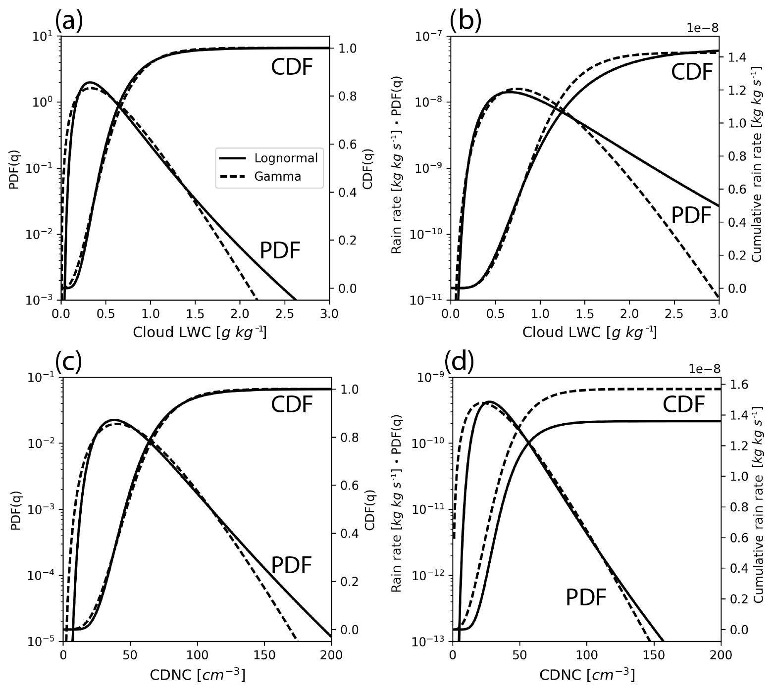
Figure 1(a) The probability density function (PDF) and cumulative distribution function (CDF) of cloud LWC (qc) that follow the gamma (dashed) and lognormal (solid) distribution. For the both distributions, 〈qc〉=0.5g kg−1 and vq=3.0. (b) The PDF and CDF of autoconversion rate computed based on the KK2000 scheme in Eq. (15) and the PDF of qc. In the computation, the Nc is kept at a constant of 50 cm−1. (c) The PDF and CDF of Nc that follow the gamma (dashed) and lognormal (solid) distribution. For the both distributions, 〈Nc〉=50 cm−3 and vN=5.0. (d) The PDF and CDF of the autoconversion rate computed based on the KK2000 scheme in Eq. (15) and the PDF of Nc. The qc is kept at 0.5 g kg−1 in the computation.
An example of the gamma and lognormal distributions for qc is shown in Fig. 1a. In this example, both distributions have the same mean 〈qc〉=0.5 g kg−1 and also the same inverse relative variance vq=3. Although the general shapes of the two PDFs are similar, they differ significantly at the two ends; the gamma PDF is larger than lognormal PDF over the small values of qc, and the opposite is true over the large values of qc. The gamma and lognormal distributions can also be used to describe the spatial variation of Nc (Gultepe and Isaac, 2004). An example is given in Fig. 1c, in which qc is a constant of 0.5 g kg−1, 〈Nc〉=50 cm−3, and vN=5.0. Figure 1b shows the autoconversion rate based on the KK2000 parameterization scheme for the gamma PG(qc) and lognormal PL(qc) that are shown in Fig. 1a. Interestingly, although the cumulative autoconversion rates based on the two types of PDFs are almost identical, the contributions to the total autoconversion rate from the different LWC bins are quite different. As shown in Fig. 1a, the PL(qc) has a longer tail than the PG(qc); i.e., the occurrence probability of large qc (e.g., qc>2.0 g kg−1) is much higher in the lognormal than in gamma PDF. This difference is further amplified in the autoconversion rate computation in Fig. 1b because the autoconversion rate is proportional to .
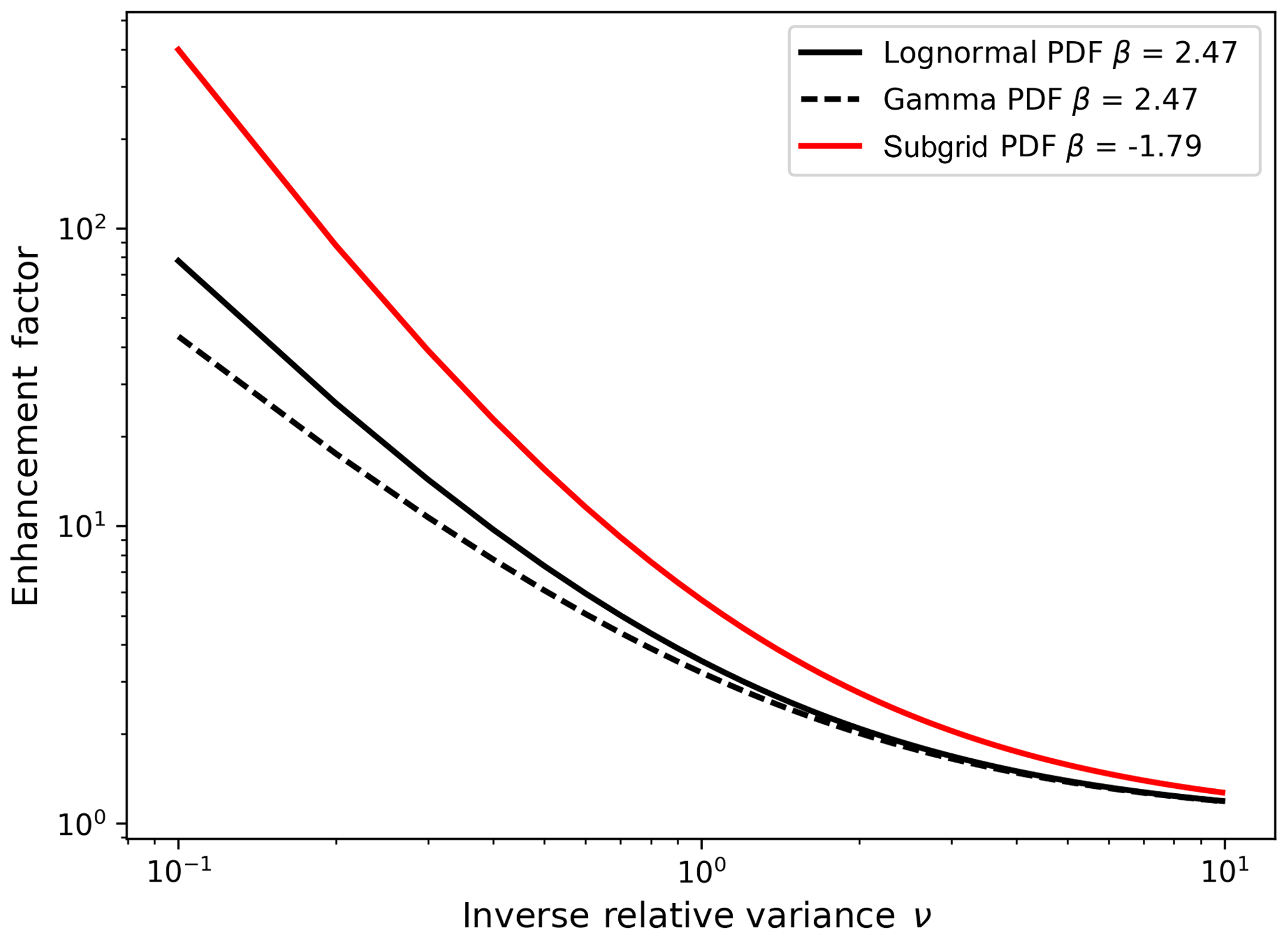
Figure 2Enhancement factors based on lognormal E(PL, β) and gamma E(PG, β) subgrid PDFs for different β as a function of the inverse relative variance v.
The enhancement factors based on the gamma (i.e., E(PG,β) in Eq. 8) and lognormal (i.e., E(PL,β) in Eq. 14) PDFs for βq=2.47 are plotted as a function of the inverse relative variance v in Fig. 2. When subgrid clouds are more homogenous, e.g., v>1, the enhancement factor based on the two PDFs are similar. However, for more inhomogeneous grids, e.g., v<1, the E(PL,β) is significantly larger than E(PG,β), which is probably because of the longer tail of PL(qc) as shown in Fig. 1a and b.
2.2 Impacts of subgrid cloud variations on warm rain parameterization in GCM
The warm rain process in MBL clouds involves many interacting microphysical processes. In this study, we focus only on the simulation of autoconversion in GCM. Other nonlinear processes, such as accretion and evaporation, have been investigated in previous studies (Boutle et al., 2014; Lebsock et al., 2013).
Ideally, if the subgrid variations of qc and Nc are known, then the grid-mean in-cloud autoconversion rate should be derived from the following integral:
where P(qc,Nc) is the joint PDF of qc and Nc. Unfortunately, most conventional GCMs lack the capability of predicting the subgrid variations of cloud properties, with only a couple of exceptions (Thayer-Calder et al., 2015). What is known from the GCM is usually the in-cloud grid-mean values 〈qc〉 and 〈Nc〉. As a result, instead of using Eq. (15), the autoconversion rate in GCMs is usually computed from the following equation:
where E is the enhancement factor defined as
The value of the enhancement factor depends on the subgrid variations of qc and Nc. If clouds are homogenous on the subgrid scale, then E∼1. In the special case where qc and Nc are independent, then the joint PDF P(qc,Nc) becomes , where P(qc) and P(Nc) are the PDF of the subgrid qc and Nc. Consequently, Eq. (15) reduces to
and Eq. (17) to
where Eq is the enhancement factor due to the subgrid variation of cloud water, which has the form
and the EN is the enhancement factor due to the subgrid variation of CDNC, which has the form
Obviously, if P(qc) and P(Nc) follow either a gamma or lognormal distribution, then the above equations reduce to Eqs. (8) or (14), respectively.
If qc and Nc both have significant subgrid variations and they are not independent, the enhancement factor should ideally be diagnosed from Eq. (17). However, the joint PDF P(qc,Nc) may not be known, and the integration can be time-consuming. Some previous studies proposed to approximate the P(qc,Nc) as a bivariate lognormal distribution as follows:
where ρ is the correlation coefficient between qc and Nc (Larson and Griffin, 2013; Lebsock et al., 2013). As such, both qc and Nc follow a marginal lognormal distribution in Eq. (9). Substituting Eq. (22) into Eq. (17), we obtain the enhancement factor for the bivariate lognormal distribution that consists of three terms:
where and EN (PL, vN, βN) = correspond to the impacts of subgrid qc and Nc variance, respectively (i.e., Eq. 14), and
corresponds to the impact of the covariation of qc and Nc on the enhancement factor. Obviously, Eq. (23) reduces to Eq. (19) when qc and Nc are uncorrelated (i.e., . If qc and Nc are negatively correlated (i.e., ρ<0 and ECOV>1), clouds with a larger qc would tend to have a smaller Nc. The autoconversion rate in such a case would be larger than that in the case where qc and Nc are positively correlated (i.e., ρ>0 and ECOV<1). A positive correlation would exist, for instance, if all droplets in clouds were the same size, but some parcels had more droplets than other parcels.
Most current GCMs do not have the capability to simulate the subgrid cloud property variations. They usually have to use predefined subgrid cloud variations in the computation of grid-mean autoconversion rate instead of using prognostic values. For example, in the MG scheme for the CAM5.3, the subgrid qc is assumed to follow the gamma distribution in Eq. (2) with a fixed vq=1 and, as a result, a constant Eq=3.2. Lately, advanced subgrid parameterization schemes, such as CLUBB, have been implemented in several GCMs, including CAM6 and GFDL AM model (Bogenschutz et al., 2018; Guo et al., 2015, 2014), which provides information on the subgrid qc variation to the host model. The information can then be used to dynamically diagnose the enhancement factor Eq, which will help the model simulate the cloud regime dependence of Eq (Guo et al., 2010, 2014).
However, as explained above, not only the subgrid variation of qc but the subgrid variation of Nc can also influence the enhancement factor. Unfortunately, this aspect has been ignored by almost all GCMs, even the latest CAM6 with CLUBB. Physically, provided the same qc, a cloud with a smaller Nc would have a larger droplet size and therefore larger precipitation efficiency than the cloud with a larger Nc. Because the autoconversion rate depends nonlinearly on Nc, the grid-mean autoconversion rate computed based on a skewed PDF of Nc (i.e., would be different from that computed based on the mean of Nc (i.e., . The autoconversion enhancement factor based on the lognormal PDF E(PL,β) for is given in Fig. 2. Interestingly, at the same inverse relative variance v, the enhancement factor based on the same lognormal PDF E(PLβ) for is actually larger than that for βq=2.47 because of the formula of the exponent in Eq. (14) (i.e., . Moreover, the correlation between Nc and qc can also be important. Going back to Eq. (23), evidently, E>Eq if and only if . After some manipulation, we can show that if βN<0 and σN>0, then
This equation reveals that when qc and Nc are weakly or negatively correlated (ρ≤0), considering only Eq would tend to underestimate E. On the other hand, however, if qc and Nc are highly positively correlated (ρ∼1), then considering Eq only would tend to overestimate E.
To derive the above-mentioned enhancement factors, we will use 10 years (2007–2016) of the latest collection 6 (C6) daily mean level-3 cloud retrieval product from the Aqua MODIS instrument (product name MYD08_D3), which contains the gridded statistics of cloud properties computed from pixel-level (i.e., level-2) retrievals. As summarized in Platnick et al. (2003, 2017), the operational level-2 MODIS cloud product provides cloud masking (Ackerman et al., 1998), cloud top height (Menzel et al., 1983), cloud top thermodynamic phase determination (Menzel et al., 2006), and COT, cloud effective radius (CER), and LWP retrievals based on the bispectral solar reflectance method (Nakajima and King, 1990). All MODIS level-2 atmosphere products, including the cloud, aerosol, and water vapor products, are aggregated to 1∘ × 1∘ spatial resolution on a daily, 8-day, and monthly basis. Aggregations include a variety of scalar statistical information, including mean, standard deviation, and max and min occurrences, as well as histograms including both marginal and joint histograms. For COT, CER, and LWP, the MODIS level-3 product provides both their in-cloud grid-mean values (〈x〉) and subgrid standard deviations (σx). The inverse relative variance v can then be derived from Eq. (5), i.e., . Note that the operational MODIS product provides two CER retrievals: one based on the observation from the band 7 centered around 2.1 µm and the other from band 20 at 3.7 µm. As discussed in several previous studies (Cho et al., 2015; Zhang and Platnick, 2011; Zhang et al., 2012, 2016), the 3.7 µm band CER retrieval is more resilient to the 3-D effects and retrieval failure than the 2.1 µm band retrievals. For these reasons, it is used as the observational reference in this study.
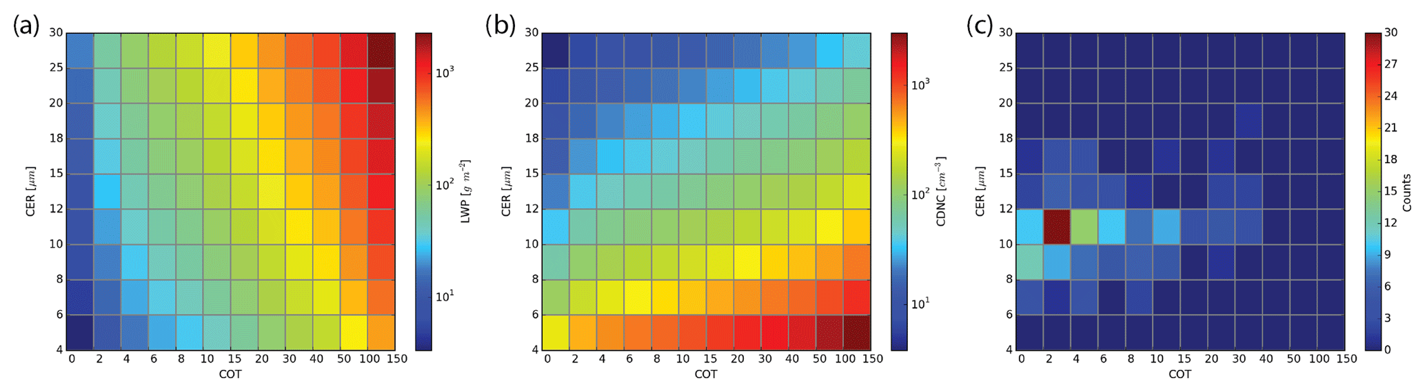
Figure 3The (a) LWP and (b) CDNC as a function of COT and CER. (c) An example of the COT–CER joint histogram observed by Aqua MODIS on 9 January 2007 at 1∘ S and 1∘ W.
Given the COT and CER retrieval, the operational MODIS product estimates the LWP of clouds using
where ρw is the density of water. Several studies have argued that a smaller coefficient of 5∕9, instead of 2∕3, should be used in estimation of LWP (Lebsock et al., 2011; Seethala and Horváth, 2010; Wood and Hartmann, 2006). The choice of coefficient does not matter in this study because it is a common factor in the calculation of v. The choice of the coefficient has no impact on our study because we are interested in the relative inverse variance . We note here that it is the LWC qc, instead of the LWP, that is used in the KK2000 scheme. So, the spatial variability of LWC is what is most relevant. However, the remote sensing of cloud water vertical profiles from satellite sensors for liquid-phase clouds is extremely challenging even with active sensors. It is why most previous studies using the satellite observations analyzed the spatial variation of LWP rather than LWC. In fact, even Lebsock et al. (2013), who used the level-2 CloudSat observations, had to use the vertically averaged LWC in their analysis. Airborne in situ measurement faces a similar challenge. For example, Boutle et al. (2014) used the LWC observation along horizontal flight tracks to study the spatial variability of cloud water, which only samples the LWC at certain levels of MBL clouds. Ground-based observations are much better than satellite and airborne observations in this regard. Recently, Xie and Zhang (2015) analyzed the cloud water profiles retrieved using ground-based radars from the three ARM sites and found no obvious in-cloud vertical dependence of the spatial variability of LWC. Following these previous studies, we assume that the horizontal subgrid variation of LWC is not strongly dependent on height, and its value can be inferred from the spatial variability of the vertically integrated quantities of LWP. The uncertainty caused by this assumption will be assessed in future studies.
The current MODIS level-3 cloud product does not provide CDNC retrievals. Following previous studies (Bennartz, 2007; Bennartz and Rausch, 2017; Grosvenor and Wood, 2014; McCoy et al., 2018), we estimate Nc of liquid-phase clouds from the MODIS-retrieved COT (τ) and CER (re) based on the classic adiabatic cloud model
where ρw is the density of water, Qe≈2 is the extinction efficiency of cloud droplets, k is the ratio of re to mean volume-equivalent radius, fad is the adiabaticity of the cloud, and Γw is the LWC lapse rate. Following previous studies, we assume k=0.8 and fad=1.0 to be constant and compute Γw from the grid-mean liquid cloud top temperature and pressure. The theoretical basis and main uncertainty sources of the CDNC estimation based on the adiabatic cloud model from MODIS-like passive cloud retrievals are nicely reviewed by Grosvenor et al. (2018).
Ideally, the values of LWP and CDNC should be estimated on a pixel-by-pixel basis from the level-2 MODIS product. However, pixel-by-pixel estimation is highly time-consuming, which makes it difficult to achieve a global perspective. Using an alternative method, many previous studies estimate the grid-level CDNC statistics from the joint histogram of COT vs. CER provided in the level-3 MODIS cloud products (Bennartz, 2007; McCoy et al., 2017, 2018). For a given 1∘ × 1∘ grid box, the liquid-phase COT–CER joint histogram provides the counts of successful cloud property retrievals with respect to 108 joint COT–CER bins that are bounded by 13 COT bin boundaries, ranging from 0 to 150, and 10 CER bin boundaries, ranging from 4 to 30 µm. With the joint histogram, which is essentially the joint PDF of COT and CER P(τre), we can estimate the grid mean and variance of CDNC from the following equations:
where x can be either LWP or CDNC. Figure 3a shows the LWP in Eq. (26) as a function of the 13 COT bins and 10 CER bins from the MODIS level-3 product. As expected, the largest LWP values are found when both COT and CER are large. Figure 3b shows the CDNC in Eq. (27) as a function of the COT and CER bins. As expected, the largest CDNC values are found when both COT is large and CER is small. Figure 3c shows an example of the COT–CER joint histogram from the Aqua MODIS daily level-3 product MYD08_D3 on 9 January 2007 at the grid box 1∘ S and 1∘ W. In this particular grid box, a combination of ∼2–4 COT and ∼10–12 µm CER is the most frequently observed cloud value. Using the joint histogram in Fig. 3c, we can derive the mean and variance of both LWP and COT using Eqs. (28) and (29).
The efficiency of using the level-3 MODIS product is accompanied by three important limitations. First of all, as mentioned earlier, MODIS provides only LWP retrievals, while LWC is needed in the KK2000 scheme. Second, the current level-3 MODIS cloud product has a fixed 1∘ × 1∘ spatial resolution. Although this resolution is highly relevant to the current generation of GCMs, i.e., Coupled Model Intercomparison Project Phase 6 (CMIP6) (Eyring et al., 2016), future GCMs may have significantly finer resolution. Third, it is difficult to subsample the pixels with the best retrieval quality. These limitations will have to be addressed in future studies.
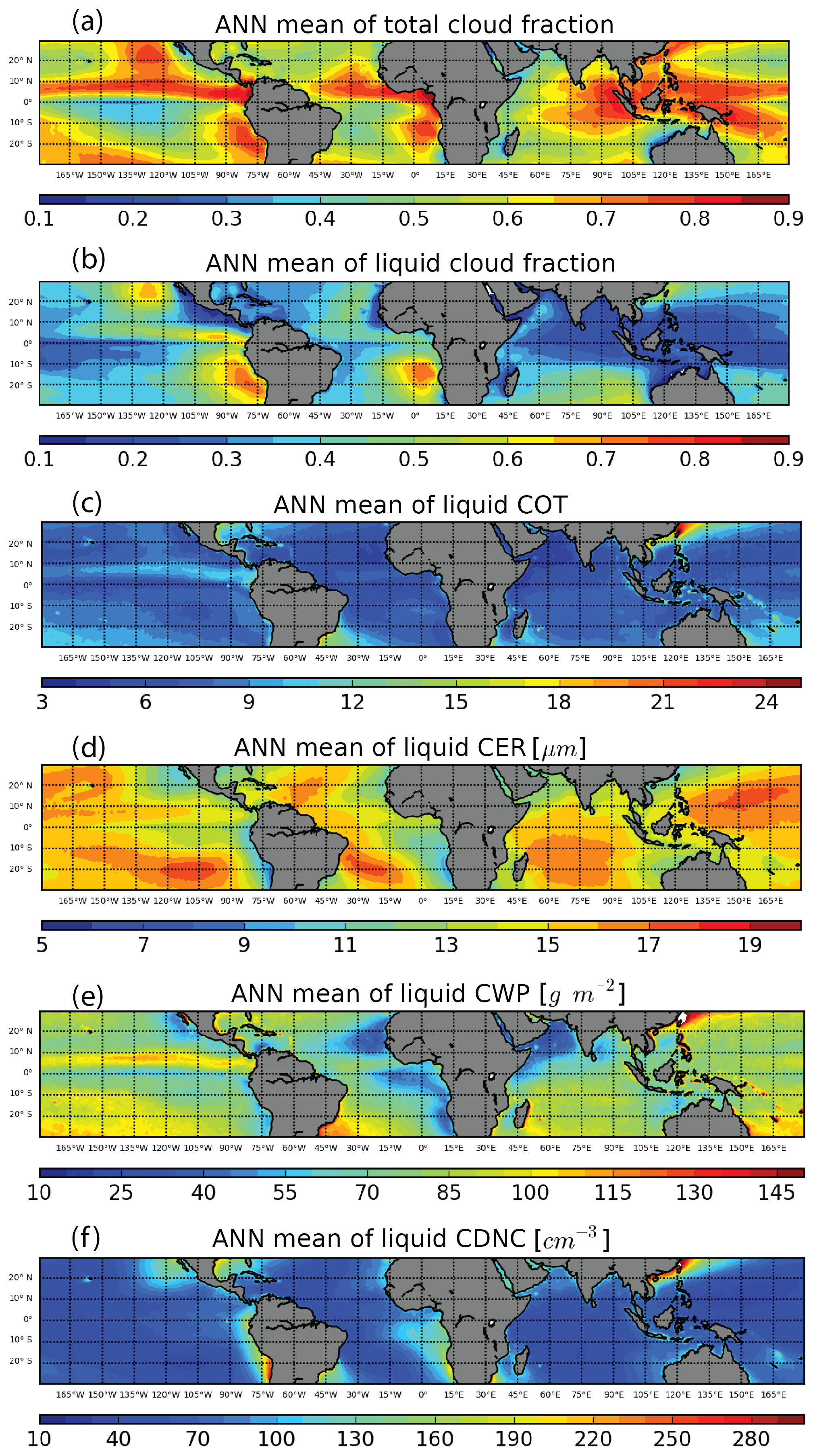
Figure 4Ten-year (2007–2016) averaged annual mean (a) total cloud fraction, (b) liquid cloud fraction, (c) cloud optical thickness, (d) cloud effective radius retrieved from the 3.7 µm band, (e) cloud water path, and (f) cloud droplet concentration retrievals from Aqua MODIS over the tropical (30∘ S–30∘ N) oceans. All quantities are in-cloud means that are averaged over the cloudy part of the grid only.
In this study, we limit our analysis to tropical oceans only where warm rain is frequent and MODIS cloud retrievals have a relatively better quality than over land or over high latitudes. The annual mean total cloud fraction (ftot), liquid-phase cloud fraction (fliq), in-cloud COT, CER from the 3.7 µm band, LWP, and estimated CDNC over the tropical oceans based on 10 years Aqua MODIS retrievals are shown in Fig. 4. The highest fliq in the tropics is usually found in the stratocumulus (Sc) decks over the eastern boundary of the ocean, e.g., the SE Pacific off the coast of Peru, the NE Pacific off the coast of California, and the SE Atlantic off the coast of Namibia. The liquid-cloud fraction reduces significantly toward the open ocean trade wind regions, where the dominant cloud types are broken cumulus (Cu). Close to the continents, the Sc decks are susceptible to the influence of the continental air mass with a higher loading of aerosols in comparison with a pristine ocean environment, which is probably the reason the SC decks have a smaller CER and higher CDNC than the open-ocean trade cumulus (Fig. 4d and f). The in-cloud COT (Fig. 4c) and LWP (Fig. 4e) generally increase from the Sc decks to the open-ocean Cu regime, although less dramatically than the transition of cloud fraction. The Sc decks and the Sc-to-Cu transition are the most prominent features of liquid-phase clouds in the tropics. However, as mentioned in the introduction, simulating these features in the GCMs proves to be an extremely challenging task, and most GCMs suffer from some common problems, such as the “too few, too bright” problem and the abrupt Sc-to-Cu transition problem (Kubar et al., 2014; Nam et al., 2012; Song et al., 2018a).
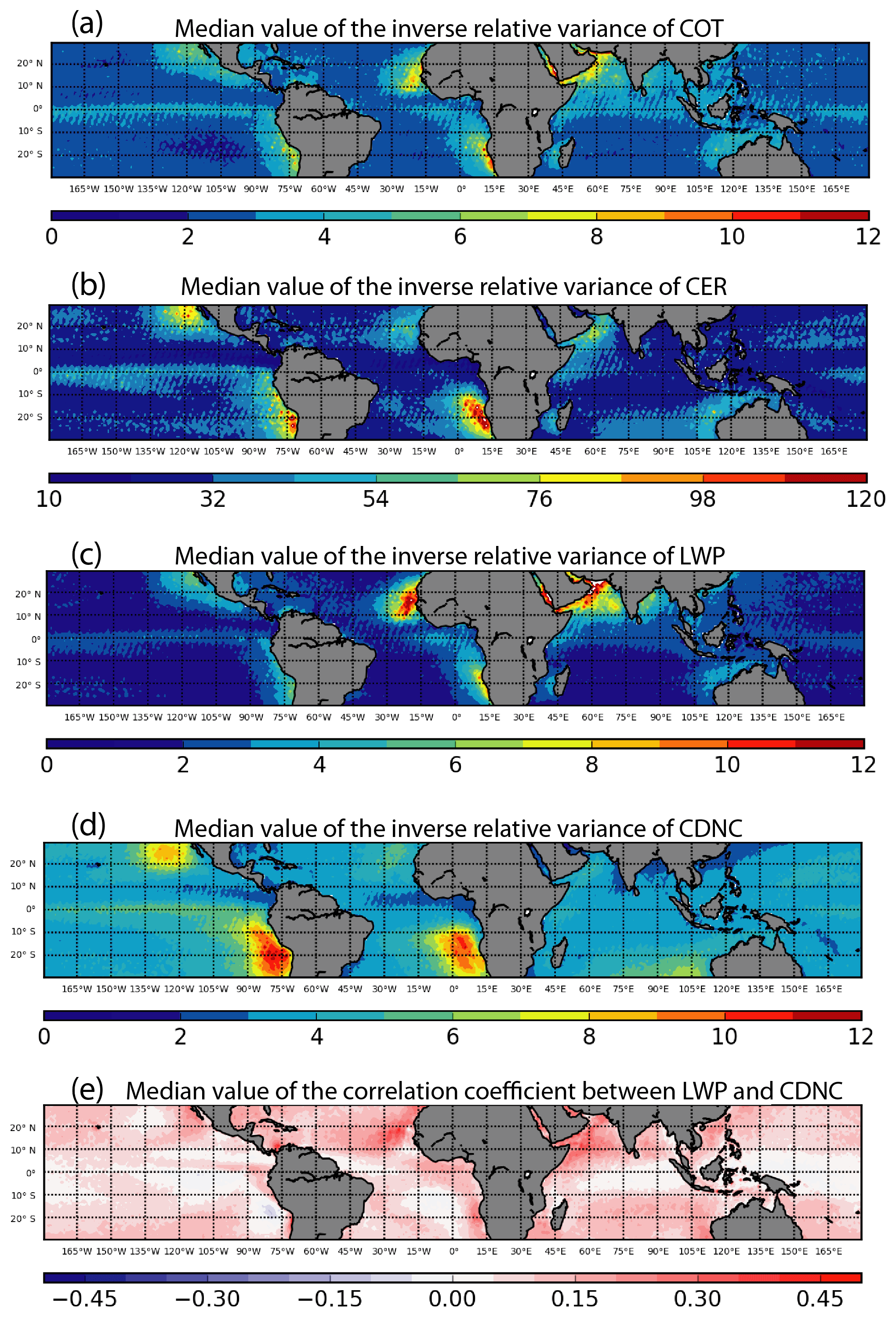
Figure 5Median value of the inverse relative variance (i.e., ) for (a) COT, (b) CER, (c) LWP, and (d) CDNC and (e) median value of the correlation coefficient between LWP and CDNC derived from 10 years of MODIS observations. Note that the color scale of CER is different from others'.
Switching the focus now from grid-mean values to subgrid variability, we will show the grid-level inverse relative variances for several key cloud properties. Here, we first derive the daily mean v and then aggregate the result to monthly mean values. Therefore, for each grid box we have 120 samples (i.e., 10 years × 12 months) of monthly mean v for analysis and visualization. Because the value of v can be ill behaved when Var(x) approaches zero, instead of the mean value, we plot the median value of based on 120 months of MODIS observations in Fig. 5. There are several interesting and important features in Fig. 5. First of all, the values of all four sets of cloud properties (i.e., COT, CER, LWP, and CDNC) all exhibit a clear and similar Sc-to-Cu transition, with larger values in the Sc regions and smaller values in the broken Cu regions. This indicates that cloud properties, including both optical and microphysical properties, are more homogenous, in terms of spatial distribution within the grid, in the Sc region than in the Cu region. Secondly, the value of of CER (i.e., 10–100 in Fig. 5b) is larger than that of the other properties (i.e., 1–10) by almost an order of magnitude, indicating that the subgrid variability of CER is very small. On the other hand, however, it is important to note that the of CDNC (Fig. 5d) is comparable with that of COT (Fig. 5a) and LWP (Fig. 5c). The reason is probably in part because the highly nonlinear relationship between CDNC and CER (i.e., ) leads to a stronger variability of CDNC than CER and also in part because the variability of CDNC is also contributed by the subgrid variation of COT. In some regions, the Gulf of Guinea, the East and South China Sea, and Bay of Bengal for example, the of CDNC is close to unity, indicating the subgrid standard deviation of CDNC is comparable to the grid-mean values in these regions. As discussed in the next section, the significant subgrid variability of CDNC in these regions should be taken into account when modeling the nonlinear processes, such as the autoconversion, in GCM to avoid systematic biases due to the nonlinearity effect.
The values of in Fig. 5 from this study are in reasonable agreement with previous studies. Barker (1996) selected a few dozens of cloud scenes, each about 100–200 km in size, from the Landsat observation and analyzed their spatial variability of COT. It is found that the typical value of v for overcast stratocumulus, broken stratocumulus, and scattered cumulus is 7.9, 1.2, and 0.7, respectively (see their Table 3), which is consistent with the Sc-to-Cu transition pattern seen in Fig. 5. Oreopoulos and Cahalan (2005) derived the subgrid inhomogeneity of COT on a global scale from the level-3 Terra MODIS retrievals. Although using a different metric (i.e., their inhomogeneity parameter is defined as ), they also found a systematic increase of inhomogeneity (decreasing value of χ) from the Sc region to Cu region. Also using the MODIS cloud property retrievals, Wood and Hartmann (2006) investigated the mesoscale spatial variability of LWP in the NE Pacific and SE Pacific regions. The v of LWP is found to increase systematically with mesoscale cloud fraction, and the relationship between the two can be reasonably explained by a simple PDF cloud thickness model in Considine et al. (1997). See also Kawai and Teixeira (2010).
As explained in Sect. 2, the correlation between cloud water and CDNC can also influence the computation of enhancement factor and thereby the grid-mean autoconversion rate. Figure 5e shows the median value of the LWP and CDNC correlation coefficient . Similar to the derivation of median , we first compute the monthly mean ρ from daily MODIS observations and then derive the median value of for each grid from the 120 months of observation. As shown in Fig. 5e, at the subgrid level, the LWP and CDNC tend to be positively correlated almost over all tropical oceans. Mathematically, this is not surprising because as shown in Fig. 5b and c, the subgrid variability of re is 1 order of magnitude smaller than that of LWP. Since CDNC is proportional to according to Eq. (27), the subgrid variability of CDNC is mainly determined by the variability of LWP, leading to the positive correlation. Physically, the correlation can be explained by several mechanisms. For example, Wood et al. (2018) and O et al. (2018) found that a large amount of low-level water clouds over the stratocumulus-to-cumulus transition are “optically thin veil clouds”. These clouds are usually associated with low LWP and low CDNC (therefore positive correlation) and probably caused by the strong precipitation scavenging process in the active cumulus. Note that our definition of ρ is the subgrid spatial correlation of LWP and CDNC. It may be different from the definition used in many aerosol indirect effect studies where the temporal correlation of monthly mean LWP and CDNC is more interesting.
5.1 Influence of subgrid variation of cloud water
As discussed in Sect. 2.2, most current GCMs only consider the impact of subgrid cloud water variation on autoconversion rate but ignore the impact of subgrid CDNC variation. To make our analysis relevant to the current GCMs, we first analyze Eq in Eq. (20) based on observations. The impacts of subgrid CDNC variation (i.e., EN) and its correlation with cloud water (i.e., ECOV) will be analyzed in the next section.
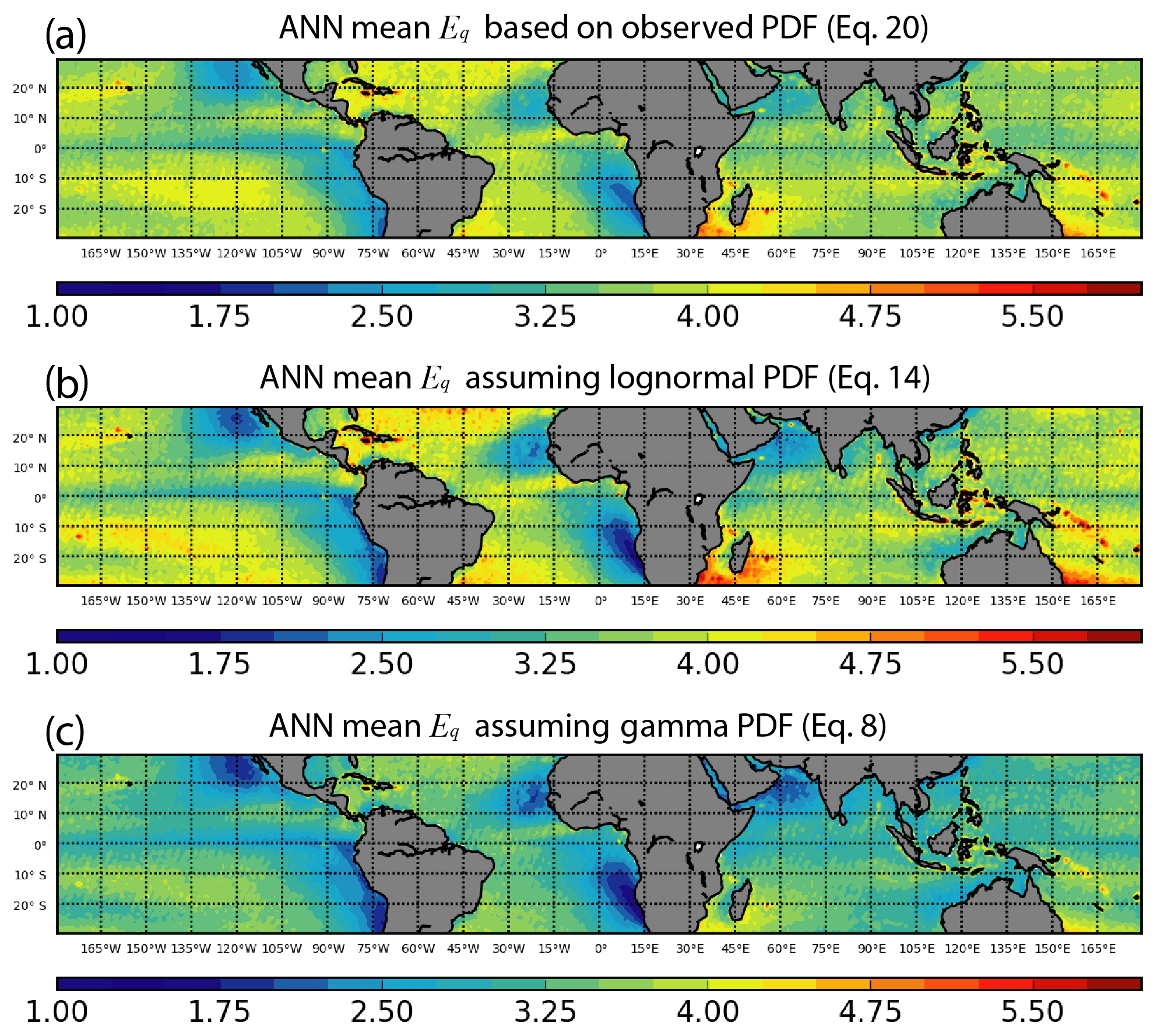
Figure 6The annual mean factor for the KK2000 scheme due to subgrid variation of LWP computed (a) directly from observation, i.e., Eq in Eq. (20), (b) from relative variance assuming lognormal PDF of LWP, i.e., Eq in Eq. (14), and (c) from relative variance assuming the gamma PDF of LWP, i.e., Eq in Eq. (8).
We derive Eq using two approaches. First, we derive it from the observed LWP PDF based on Eq. (20). As such, we do not have to make any assumptions about the shape of LWP PDF, although solving the integration in Eq. (20) is time-consuming. In the second approach, we first derive the relative inverse relative variance v of LWP and then derive the enhancement factor by assuming the subgrid PDF to be either gamma or lognormal. This approach is more efficient, but it may be subject to error if the true PDF deviates from the assumed PDF shape. Figure 6a shows the annual mean enhancement factor Eq in the tropical region derived based on Eq. (20) (i.e., the first approach) from 10 years of MODIS observations. Figure 6b and c show the annual mean enhancement factor Eq derived by assuming the subgrid cloud water follows the lognormal (i.e., Eq. 14) and gamma distribution (i.e., Eq. 8), respectively. There are a couple of interesting and important points to note. First of all, similar to the grid-mean quantities in Fig. 4, the enhancement factor Eq also shows a clear Sc-to-Cu transition. Over the Sc decks, because clouds are more homogeneous (), the enhancement factor Eq is only around 1–2.5, while over the Cu regions, the more inhomogeneous clouds with leads to a larger enhancement factor Eq around 3–5. As mentioned previously, in the current CAM5.3, Eq is assumed to be a constant of 3.2. While this value is within the observational range, it obviously cannot capture the Sc-to-Cu transition. In fact, the constant value 3.2 overestimates the Eq over the Sc region and underestimates the Eq over the Cu region, which could lead to unrealistic drizzle production in both regions and to consequential impacts on cloud water budget, radiation, and even aerosol indirect effects on the model. The second point to note is that the Eq based on the lognormal PDF assumption in Fig. 6b agrees well with the results in Fig. 6a derived directly from the observation. In contrast, the Eq based on the gamma PDF assumption in Fig. 6c tends to be smaller, especially in the Cu regions. This result seems to suggest that the lognormal distribution provides a better fit to the observed subgrid cloud water variation than the gamma distribution, which has rarely been noted and reported in the previous studies.
A flexible, cloud-regime-dependent Eq could help improve the simulation of Sc-to-Cu transition in the GCM. If a GCM employs an advanced cloud parameterization scheme, such as CLUBB, that is able to provide regime-dependent information on subgrid cloud variation, i.e., v, then the enhancement factor Eq could be diagnosed from v. However, most traditional cloud parameterization schemes do not provide information on subgrid cloud variation. In such cases, if one does not wish to use a constant Eq but a varying regime-dependent scheme, then either v or Eq need to be parameterized as a function of some grid-mean cloud properties resolved by the GCM. In fact, several attempts have been made along this line. Based on the combination airborne in situ measurements and satellite remote sensing products, Boutle et al. (2014) parameterized the “fractional standard deviation” (which is equivalent to in our definition) of liquid-phase cloud as a function of grid-mean cloud fraction. This scheme was later updated and tested in a host GCM in Hill et al. (2015) and was found to reduce the shortwave cloud radiative forcing biases in the model. In a recent study, Xie and Zhang (2015) derived the subgrid cloud variations from the ground-based observations from three DOE ARM sites, and then parameterized the inverse relative variance v as a function of the atmospheric stability.
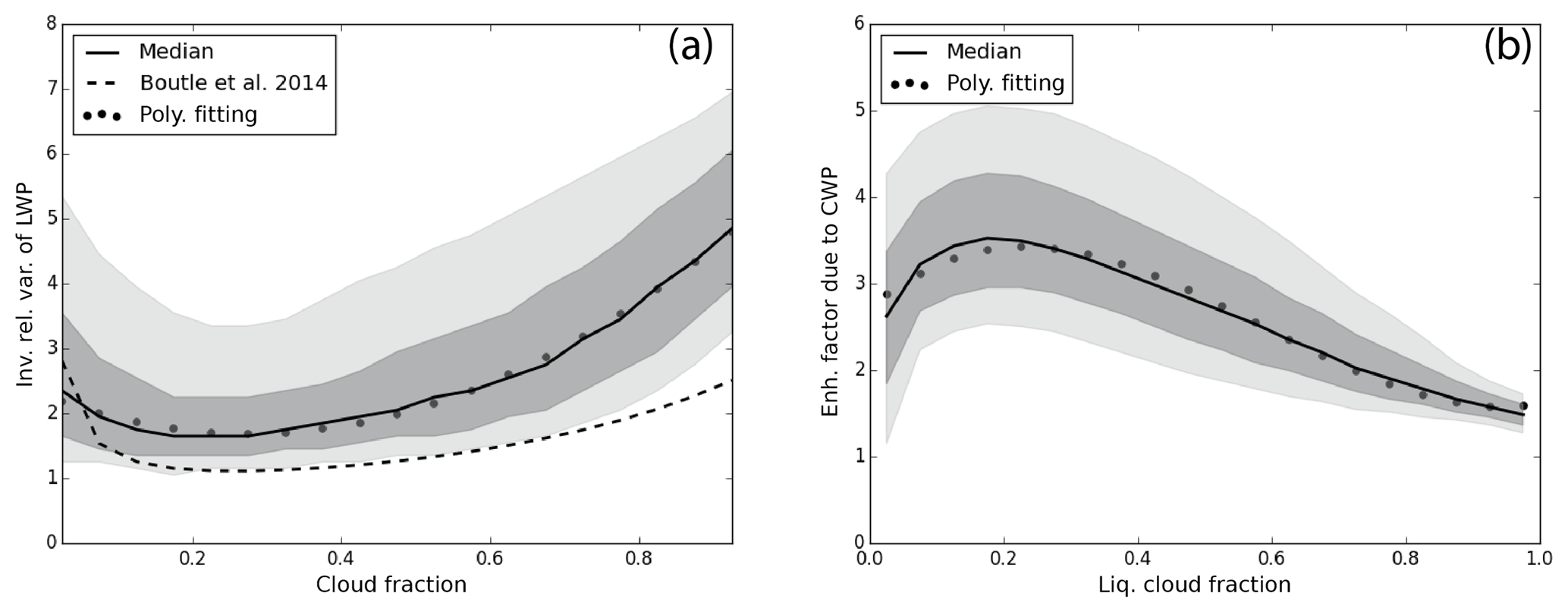
Figure 7(a) The inverse relative variance v and (b) autoconversion enhancement factor due to LWP subgrid variability assuming lognormal PDF as a function of grid-mean liquid cloud fraction, where the solid line, dark shaded area, and light shaded area correspond to the median value, 25 %–75 % percentiles, and 10 %–90 % percentiles, respectively. The dotted lines correspond to simple third-order polynomial fitting. For reference, the vq(fliq) parameterization scheme based on Boutle et al. (2014) is also plotted in panel (a).
Figure 7a shows the variation of inverse relative variance v as a function of the grid-mean liquid-phase cloud fraction fliq. In general, the value of v increases with the increasing fliq, which is expected from the Sc-to-Cu increase of fliq in Fig. 4b and the Sc-to-Cu decrease of v in Fig. 5c. The v(fliq) pattern in Fig. 7a is also consistent with the results reported in Wood and Hartmann (2006) and Lebsock et al. (2013). In the hope of obtaining a simple parameterization scheme for v(fliq) that can be used in GCMs, we fit the median value of v as a simple third-order polynomial of fliq as follows:
For comparison, we also plotted the v(fliq) parameterization developed by Boutle et al. (2014) for grid size of 100 km (dashed line in the figure). Apparently, comparing with Eq. (30), it generates slightly smaller v for a given the fliq. This difference is probably because our results are based on different data.
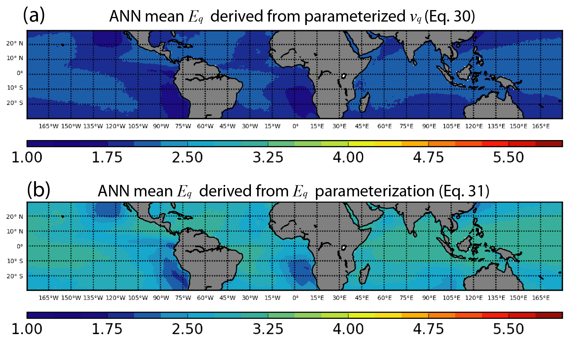
Figure 8Annual mean value of the enhancement factor EN computed based on the (a) parameterization scheme in Eq. (30) and (b) parameterization scheme in Eq. (31).
To test the performance of this simple parameterization, we first substitute the fliq from the MODIS daily mean level-3 product into the above equation and then use the resultant v to compute the enhancement factor Eq. Unfortunately, the enhancement factor Eq computed based on the parameterized v(fliq) as shown in Fig. 8a substantially underestimates the observation-based results in Fig. 6, especially over the Cu regions. The deviation is probably because the relationship between Eq and v is highly nonlinear (e.g., Eqs. 8 and 14), and therefore the above parameterization scheme that is designed for v is not able to capture the variability of Eq. Based on this consideration, we tried an alternative approach. Instead of parameterization of v, we directly parameterize the enhancement factor Eq as a function of fliq. Figure 7b shows the variation of Eq as a function of fliq. As expected, Eq generally decreases with increasing fliq. The median value of Eq is fitted with the following third-order polynomial of fliq:
As shown in Fig. 8b, the value of Eq based on the above equation clearly agrees with the observation-based values in Fig. 6 better than that based on the parameterization of v(fliq). The elimination of the middle step indeed improves the parameterization results. While this is encouraging, it should be kept in mind that Eq. (31) has very limited application; i.e., it is only useful for the autoconversion rate computation for a particular value of the autoconversion exponent beta, i.e., βq=2.47. A good parameterization of v could be useful not only for autoconversion, but also for accretion and radiation computations. Another caution is that, if applied to a GCM, the performance of the Eq(fliq) parameterization in Eq. (31) will be dependent on the simulated accuracy of fliq in the model.
5.2 Influence of subgrid variance of CDNC
Now we will investigate the impacts of subgrid CDNC variation on the autoconversion rate simulation. For the moment, we will consider EN only. The impact of CDNC and cloud water correlation will be discussed in the next section. Similar to Eq we first derive EN from the CDNC PDF based on Eq. (21). The annual mean result based on 10 years of MODIS observations is shown in Fig. 9a. There are several intriguing points to note. First of all, the value of EN is actually larger than Eq in Fig. 9 such that we even have to use a different color scale for this plot. Secondly, the regions with escalated EN seem to coincide with the downwind regions of biomass burning aerosols (e.g., Gulf of Guinea, east coast of South Africa), air pollution (i.e., East China Sea), and, most interestingly, active volcanos (e.g., Kilauea, Hawaii, and Ambae, Vanuatu). We have also checked the seasonal variation of the EN and the results also support this observation. Another interesting feature to note is that, although the dust outflow regions, such as the tropical East Atlantic and Arabian Sea, have heavy aerosol loading, the value of EN there is only moderate. Figure 9b shows the value of EN computed based on Eq. (14) from the inverse relative variance of v, assuming that the subgrid CDNC follows a lognormal PDF. Although the overall pattern is consistent with Fig. 9a, the assumption of the lognormal PDF seems to underestimate EN. A closer examination indicates that the lognormal PDF tends to underestimate the population of clouds with a small CDNC and therefore underestimate the variance of CDNC as well as EN. We did not compute the EN based on the gamma distribution because of the singular value problem mentioned in Sect. 2.1.
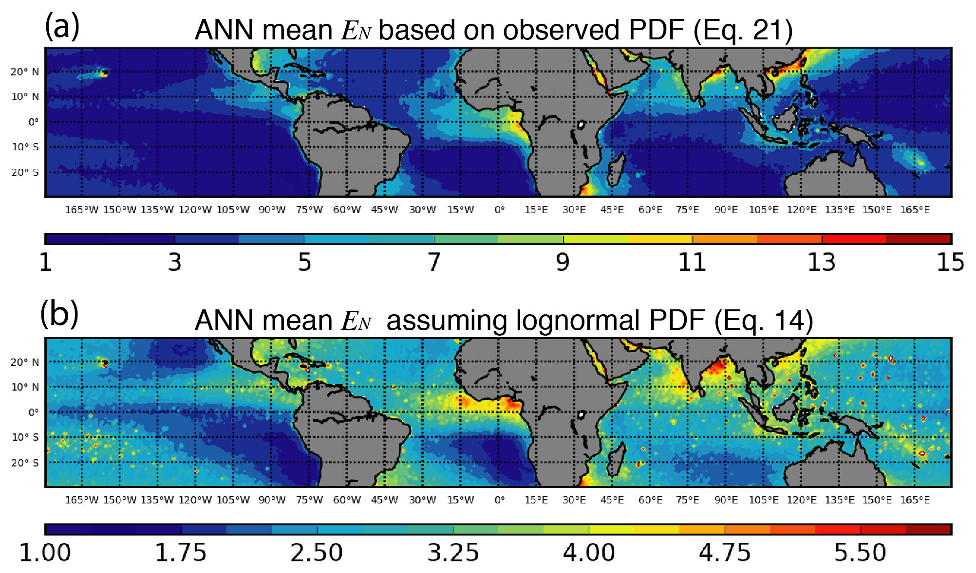
Figure 9Annual mean value of the enhancement factor EN derived from (a) observation based on Eq. (21) and (b) from Eq. (14) assuming lognormal subgrid CDNC distribution.
We could not find any previous observation-based study on the global pattern of the subgrid variation of CDNC and the corresponding EN. So, it is difficult for us to corroborate our results. On the one hand, the magnitude of EN is surprisingly large. As explained in Sect. 3, the CDNC is estimated based on Eq. (27) from the MODIS retrieval of COT and CER. Several previous studies have shown that the subpixel-level surface contamination, subpixel cloud inhomogeneity, and three-dimensional radiative transfer effects can cause significant errors in the MODIS CER retrievals, especially over broken cloud regions (Zhang and Platnick, 2011; Zhang et al., 2012, 2016). Given the fact that the CDNC retrieval is highly sensitive to CER error as a result of , the influence of retrieval uncertainty on subgrid CDNC variation cannot be ruled out. On the other hand, the pattern of EN in Fig. 9a seems to suggest that there are some underlying physical mechanisms controlling the subgrid variation of CDNC, in which aerosols seem to play an important role. To achieve a better understanding, we analyzed the dependence of EN on liquid cloud fraction and grid-mean CDNC in Fig. 10, which reveals that EN has a stronger dependence on CDNC than cloud fraction. This result seems to indicate that the pattern of EN in Fig. 9 is largely determined by physical mechanisms rather than retrieval uncertainties. Interestingly, the largest EN is usually found when liquid cloud fraction is small and CDNC is large and decreases with decreasing CDNC and increasing cloud fraction. This pattern leads us to the following hypothesis: In the regions where aerosol is limited, even weak updrafts can activate most cloud condensation nuclei (CCN). As a result, even if there is significant subgrid variation of turbulence at cloud base, the subgrid variation of CDNC remains small. In contrast, in regions where aerosol is abundant, the subgrid variation of turbulence becomes important. The subgrid variation of updraft leads to subgrid variation CDNC and thereby a large EN.
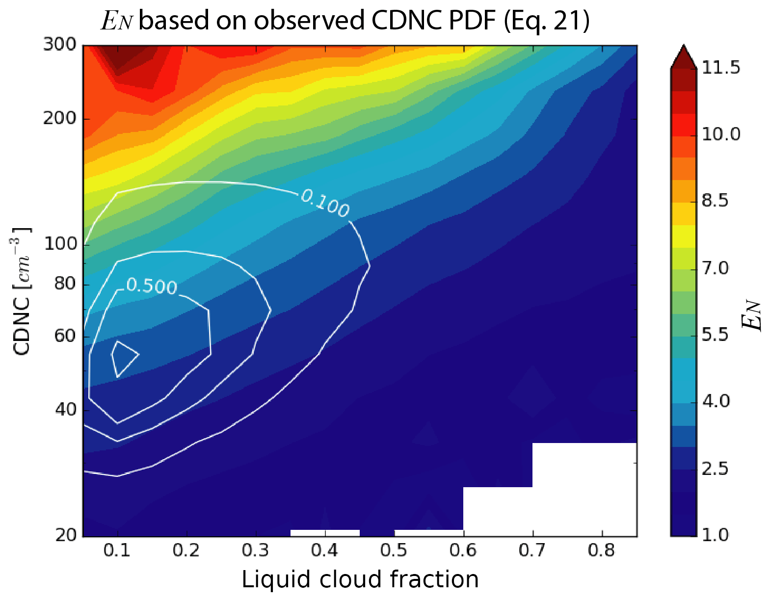
Figure 10Dependence of EN on fliq and Nd. The color map corresponds to the mean value of EN for a given Nd and fliq bin. The white contour lines correspond to the relative sampling frequency of Nd and fliq bins (i.e., the most frequently observed combination is Nd∼50 cm−3 and fliq∼0.1).
As far as we know, the results in Figs. 9 and 10 mark the first attempt based on satellite observations to unveil the global pattern of the subgrid variations of CDNC and investigate the consequential impacts on warm rain simulations in GCMs. Although obscured by satellite retrieval uncertainties, the results still provide valuable insights. First of all, the enhancement factor EN due to the subgrid variations of CDNC is non-negligible, even comparable to the effect of subgrid cloud water variation (i.e., Eq). Second, the global pattern of EN in Fig. 9 provides a valuable map for future studies.
5.3 The combined effect of subgrid variations of cloud water and CDNC
Finally, in this section we examine the combined effect of subgrid variations of cloud water and CDNC, as well as their correlation, on the autoconversion rate simulation. The annual mean combined enhancement factor E derived based on Eq. (17) from 10 years of MODIS COT and CER observations is shown in Fig. 11a. Comparing with the Eq in Fig. 6 and EN in Fig. 9, the combined enhancement factor is generally larger. It is easy to see that in some regions (e.g., Gulf of Guinea, east coast of South Africa, and East China Sea), the combined enhancement factor E resembles EN, while in other regions (i.e., trade wind cumulus regions over open ocean) it resembles more of Eq. Interestingly, because both Eq and EN are small over the Sc decks, those regions have the smallest combined enhancement factor E. As discussed in Sect. 2.2, only when the subgrid variation of cloud water is uncorrelated with the subgrid variation of CDNC can the combined enhancement factor E be decomposed into the simple product of Eq and EN (i.e., Eq. 19). Figure 11b shows the annual mean value of the simple product Eq⋅EN, without considering the correlation between cloud water and CDNC. Evidently, the simple product substantially overestimates the combined enhancement factor derived from the joint PDF of LWP and CDNC. This result can be explained by the mostly positive subgrid correlation between LWP and CDNC in Fig. 5e. As explained in Sect. 2.2, the positive correlation means that clouds with more water also tend to have more CDNC. The autoconversion rate of such configurations is lower than that when LWP and CDNC have no correlation.
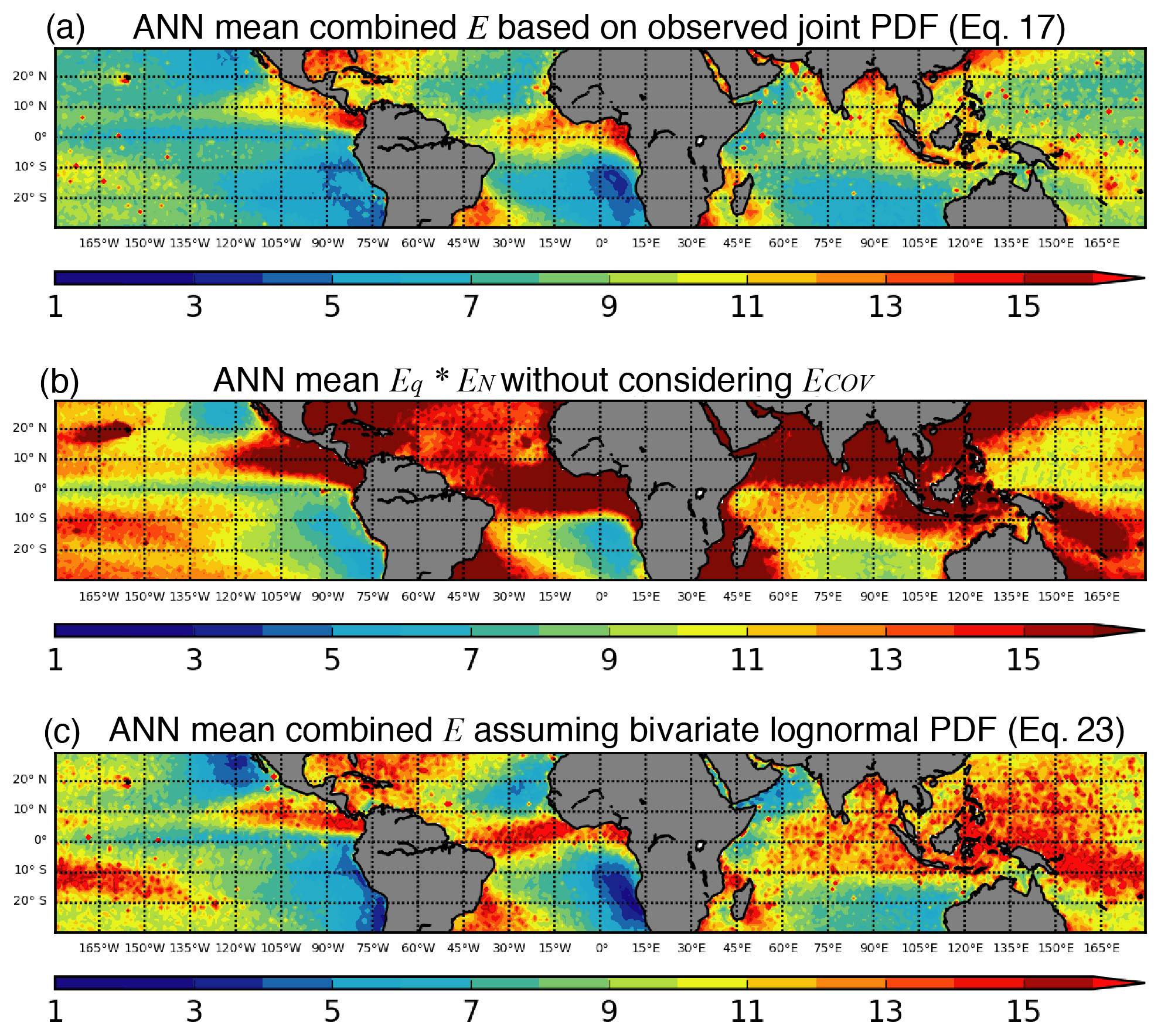
Figure 11The combined enhancement factor derived (a) based on Eq. (17) from the observed joint PDF of LWP and CDNC, (b) assuming that subgrid variations of LWP and CDNC are uncorrelated, i.e., Eq⋅EN only, and (c) based on Eq. (23) assuming that the subgrid LWP and CDNC following the bivariate lognormal distribution.
Together, the Eq in Fig. 6, EN in Fig. 9, and the combined enhancement factor in Fig. 11 lead us to the following important conclusion. It is not sufficient to consider only the impact of subgrid variation of cloud water (i.e., Eq) on the autoconversion rate simulation. The influences of subgrid CDNC variation, as well as the correlation between cloud water and CDNC, must also be taken into account to avoid significant error.
Finally, the combined enhancement factor derived based on Eq. (23), assuming that the LWP and CDNC follow the bivariate lognormal distribution, is shown in Fig. 11c. Despite the tendency of overestimation, the result agrees reasonably well with that based on observed joint PDFs in Fig. 11a, clearly better than the simple product Eq⋅EN. This is encouraging as it suggests that the bivariate lognormal distribution can be used in the future to model the combined effect of cloud water and CDNC on autoconversion rate simulation in GCMs.
One of the difficulties in GCM simulation of the warm rain parameterization is how to account for the impact of subgrid variations of cloud properties, such as cloud water and CDCN, on nonlinear precipitation processes such as autoconversion. In practice, this impact is often treated by adding the enhancement factor term to the parameterization scheme. In this study, we derived the subgrid variations of liquid-phase cloud properties over the tropical ocean using the satellite remote sensing products from MODIS and investigated the corresponding enhancement factors for parameterizations of autoconversion rate. In comparison with previous work, our study is able to shed some new light on this problem in the following regards.
-
A theoretical framework is presented to explain the importance of the subgrid variation of CDNC and its correlation with cloud water on the autoconversion rate simulation in GCMs.
-
The wide spatial coverage of the level-3 MODIS product enables us to depict a detailed quantitative picture of the enhancement factor Eq, which shows a clear cloud regime dependence, i.e., a Sc-to-Cu increase. The constant Eq=3.2 used in the current CAM5.3 model overestimates and underestimates the observed Eq in the Sc and Cu regions, respectively.
-
The Eq based on the lognormal PDF assumption performs significantly better than that based on the gamma PDF assumption. A simple parameterization scheme is provided to relate Eq to the grid-mean liquid cloud fraction, which can be readily used in GCMs.
-
For the first time, the enhancement factor EN due to the subgrid variation of CDNC is derived from satellite observation, and the results reveal several regions downwind of biomass burning aerosols (e.g., Gulf of Guinea, east coast of South Africa), air pollution (i.e., East China Sea), and active volcanos (e.g., Kilauea, Hawaii, and Ambae, Vanuatu). The largest EN is usually found where CDNC is large and liquid cloud fraction is small and decreases with decreasing CDNC and increasing cloud fraction.
-
MODIS observations suggest that the subgrid LWP and CDNC are mostly positively correlated. As a result, the combined enhancement factor is significantly smaller than the simple product of Eq⋅EN (i.e., assuming no correlation). The combined enhancement factor derived assuming LWP and CDNC follow the bivariate lognormal distribution agrees with the observation-based results reasonably well.
As noted in the previous sections, this study has several important limitations, most of which are a result of using the level-3 MODIS observations. The fixed 1∘ × 1∘ spatial resolution of the MODIS level-3 product makes it impossible for us to investigate the scale dependence of subgrid cloud variation. Similar to previous studies, we have to make several assumptions when estimating the CDNC from the level-3 MODIS product. Furthermore, the retrieval uncertainties associated with the optically thin clouds in the MODIS product pose a challenging obstacle for the quantification of subgrid cloud property variations and the corresponding enhancement factors. These limitations have to be addressed using additional independent observations from, for example, ground-based remote sensing products and/or in situ measurements from airborne field campaigns. Recently, a few novel methods have been developed to provide certain information on the subgrid cloud property variations to the host GCM. Most noticeable examples are the super-parameterization method (a.k.a. multiscale modeling framework) (Wang et al., 2015) and the PDF-based higher-order turbulence closure methods, e.g., Cloud Layer Unified By Binormals (CLUBB) (Golaz et al., 2002a; Guo et al., 2015; Larson et al., 2002) and Eddy-Diffusivity Mass Flux (EDMF) (Sušelj et al., 2013). The subgrid cloud property variations derived in this study provide the valuable observational basis for the evaluation and improvement of these schemes.
The MODIS level-3 daily averaged products used in this study are available from the Level-1 and Atmosphere Archive and Distribution System (LAADS) Distributed Active Archive Center (DAAC) of NASA. All results from the analysis can be made available upon request to the corresponding author.
ZZ conceived the idea, performed most of the analyses, and drafted the manuscript. HS helped with the data analysis and figures. PLM and VEL helped with the preparation and revision of the manuscript. MW, XD, and JW all participated in the project and helped with this study.
The authors declare that they have no conflict of interest.
Zhibo Zhang acknowledges the financial support from the
Regional and Global Climate Modeling program (grant no. DE-SC0014641) funded
by the Biological and Environmental Research program in the US DOE, Office of
Science. This work is also supported by the grant CyberTraining: DSE:
Cross-Training of Researchers in Computing, Applied Mathematics and
Atmospheric Sciences using Advanced Cyberinfrastructure Resources from the
National Science Foundation (grant no. OAC–1730250). Po-Lun Ma was support
by the US DOE, Office of Science, Biological and Environmental Research
program and Regional and Global Model Analysis program. The Pacific Northwest
National Laboratory is operated for the DOE by Battelle Memorial Institute
under contract DE-AC05-76RL01830. Vincent E. Larson is grateful for financial
support from Climate Model Development and Validation (grant no.
DE-SC0016287), which is funded by the Biological and Environmental Research
program in the US DOE, Office of Science. Minghuai Wang was supported by the
Ministry of Science and Technology of China (grant no. 2017YFA0604001). The
computations in this study were performed at the UMBC High Performance
Computing Facility (HPCF). The facility is supported by the US National
Science Foundation through the MRI program (grant nos. CNS-0821258 and
CNS-1228778) and the SCREMS program (grant no. DMS-0821311), with substantial
support from UMBC.
Edited by: Xiaohong
Liu
Reviewed by: Ian Boutle, Matthew Lebsock, and one
anonymous referee
Ackerman, S., Strabala, K., Menzel, W., Frey, R., Moeller, C., and Gumley, L.: Discriminating clear sky from clouds with MODIS, J. Geophys. Res., 103, 32141–32157, 1998.
Ahlgrimm, M. and Forbes, R. M.: Regime dependence of cloud condensate variability observed at the Atmospheric Radiation Measurement Sites, Q. J. Roy. Meteor. Soc., 142, 1605–1617, https://doi.org/10.1002/qj.2783, 2016.
Barker, H. W.: A Parameterization for Computing Grid-Averaged Solar Fluxes for Inhomogeneous Marine Boundary Layer Clouds. Part I: Methodology and Homogeneous Biases, J. Atmos. Sci., 53, 2289–2303, https://doi.org/10.1175/1520-0469(1996)053<2289:APFCGA>2.0.CO;2, 1996.
Barker, H. W., Wiellicki, B. A., and Parker, L.: A Parameterization for Computing Grid-Averaged Solar Fluxes for Inhomogeneous Marine Boundary Layer Clouds. Part II: Validation Using Satellite Data, J. Atmos. Sci., 53, 2304–2316, https://doi.org/10.1175/1520-0469(1996)053<2304:APFCGA>2.0.CO;2, 1996.
Bennartz, R.: Global assessment of marine boundary layer cloud droplet number concentration from satellite, J. Geophys. Res.-Atmos., 112, D02201, https://doi.org/10.1029/2006JD007547, 2007.
Bennartz, R. and Rausch, J.: Global and regional estimates of warm cloud droplet number concentration based on 13 years of AQUA-MODIS observations, Atmos. Chem. Phys., 17, 9815–9836, https://doi.org/10.5194/acp-17-9815-2017, 2017.
Bogenschutz, P. A., Gettelman, A., Morrison, H., Larson, V. E., Craig, C., and Schanen, D. P.: Higher-Order Turbulence Closure and Its Impact on Climate Simulations in the Community Atmosphere Model, J. Climate, 26, 9655–9676, https://doi.org/10.1175/JCLI-D-13-00075.1, 2013.
Bogenschutz, P. A., Gettelman, A., Hannay, C., Larson, V. E., Neale, R. B., Craig, C., and Chen, C.-C.: The path to CAM6: coupled simulations with CAM5.4 and CAM5.5, Geosci. Model Dev., 11, 235–255, https://doi.org/10.5194/gmd-11-235-2018, 2018.
Bony, S. and Dufresne, J.-L.: Marine boundary layer clouds at the heart of tropical cloud feedback uncertainties in climate models, Geophys. Res. Lett., 32, L20806, https://doi.org/10.1029/2005GL023851, 2005.
Boutle, I. A., Abel, S. J., Hill, P. G., and Morcrette, C. J.: Spatial variability of liquid cloud and rain: observations and microphysical effects, Q. J. Roy. Meteor. Soc., 140, 583–594, https://doi.org/10.1002/qj.2140, 2014.
Cahalan, R. F., Ridgway, W., Wiscombe, W. J., Bell, T. L., and Snider, J. B.: The Albedo of Fractal Stratocumulus Clouds, J. Atmos. Sci., 51, 2434–2455, https://doi.org/10.1175/1520-0469(1994)051<2434:TAOFSC>2.0.CO;2, 1994.
Cho, H. M., Zhang, Z., Meyer, K., Lebsock, M., Platnick, S., Ackerman, A. S., Di Girolamo, L., C.-Labonnote, L., Cornet, C., Riedi, J., and Holz, R. E.: Frequency and causes of failed MODIS cloud property retrievals for liquid phase clouds over global oceans, J. Geophys. Res.-Atmos., 120, 2015JD023161, https://doi.org/10.1002/2015JD023161, 2015.
Considine, G., Curry, J. A., and Wielicki, B.: Modeling cloud fraction and horizontal variability in marine boundary layer clouds, J. Geophys. Res., 102, 13517–13525, 1997.
Eyring, V., Bony, S., Meehl, G. A., Senior, C. A., Stevens, B., Stouffer, R. J., and Taylor, K. E.: Overview of the Coupled Model Intercomparison Project Phase 6 (CMIP6) experimental design and organization, Geosci. Model Dev., 9, 1937–1958, https://doi.org/10.5194/gmd-9-1937-2016, 2016.
Golaz, J.-C., Larson, V. E., and Cotton, W. R.: A PDF-Based Model for Boundary Layer Clouds. Part I: Method and Model Description, JAS, 59(24), 3540–3551, https://doi.org/10.1175/1520-0469(2002)059< 3540:APBMFB>2.0.CO;2, 2002a.
Golaz, J.-C., Larson, V. E., and Cotton, W. R.: A PDF-Based Model for Boundary Layer Clouds. Part II: Model Results, J. Atmos. Sci., 59, 3552–3571, https://doi.org/10.1175/1520-0469(2002)059<3552:APBMFB>2.0.CO;2, 2002b.
Griffin, B. M. and Larson, V. E.: Analytic upscaling of a local microphysics scheme. Part II: Simulations, Q. J. Roy. Meteor. Soc., 139, 58–69, https://doi.org/10.1002/qj.1966, 2013.
Grosvenor, D. P. and Wood, R.: The effect of solar zenith angle on MODIS cloud optical and microphysical retrievals within marine liquid water clouds, Atmos. Chem. Phys., 14, 7291–7321, https://doi.org/10.5194/acp-14-7291-2014, 2014.
Grosvenor, D. P., Sourdeval, O., Zuidema, P., Ackerman, A., Alexandrov, M. D., Bennartz, R., Cairns, B., Chiu, C., Christensen, M., Diamond, M., Feingold, G., Fridlind, A., Hunerbein, A., Knist, C., Kollias, P., Marshak, A., McCoy, D., Merk, D., Painemal, D., Rausch, J., Rosenfeld, D., Russchenberg, H., Seifert, P., Sinclair, K., Stier, P., vanDiedenhoven, B., Wendisch, M., Werner, F., Wood, R., Zhang, Z., and Quaas, J.: Remote sensing of droplet number concentration in warm clouds: A review of the current state of knowledge and perspectives, Rev. Geophys., 56, 409–453, https://doi.org/10.1029/2017RG000593, 2018.
Gultepe, I. and Isaac, G. A.: Aircraft observations of cloud droplet number concentration: Implications for climate studies, Q. J. Roy. Meteor. Soc., 130, 2377–2390, https://doi.org/10.1256/qj.03.120, 2004.
Guo, H., Golaz, J.-C., Donner, L. J., Larson, V. E., Schanen, D. P., and Griffin, B. M.: Multi-variate probability density functions with dynamics for cloud droplet activation in large-scale models: single column tests, Geosci. Model Dev., 3, 475–486, https://doi.org/10.5194/gmd-3-475-2010, 2010.
Guo, Z., Wang, M., Qian, Y., Larson, V. E., Ghan, S., Ovchinnikov, M., Bogenschutz, P. A., Zhao, C., Lin, G., and Zhou, T.: A sensitivity analysis of cloud properties to CLUBB parameters in the single-column Community Atmosphere Model (SCAM5), J. Adv. Model. Earth Sy., 6, 829–858, https://doi.org/10.1002/2014MS000315, 2014.
Guo, H., Golaz, J. C., Donner, L. J., Wyman, B., Zhao, M., and Ginoux, P.: CLUBB as a unified cloud parameterization: Opportunities and challenges, Geophys. Res. Lett., 42, 4540–4547, https://doi.org/10.1002/2015GL063672, 2015.
Hill, P. G., Morcrette, C. J., and Boutle, I. A.: A regime-dependent parametrization of subgrid-scale cloud water content variability, Q. J. Roy. Meteor. Soc., 141, 1975–1986, https://doi.org/10.1002/qj.2506, 2015.
Kawai, H. and Teixeira, J.: Probability Density Functions of Liquid Water Path and Cloud Amount of Marine Boundary Layer Clouds: Geographical and Seasonal Variations and Controlling Meteorological Factors, J. Climate, 23, 2079–2092, https://doi.org/10.1175/2009JCLI3070.1, 2010.
Khairoutdinov, M. and Kogan, Y.: A New Cloud Physics Parameterization in a Large-Eddy Simulation Model of Marine Stratocumulus, Mon. Weather Rev., 128, 229–243, 2000.
Klein, S. and Hartmann, D.: The seasonal cycle of low stratiform clouds, J. Climate, 6, 1587–1606, 1993.
Kubar, T. L., Stephens, G. L., Lebsock, M., Larson, V. E., and Bogenschutz, P. A.: Regional Assessments of Low Clouds against Large-Scale Stability in CAM5 and CAM-CLUBB Using MODIS and ERA-Interim Reanalysis Data, J. Climate, 28, 1685–1706, https://doi.org/10.1175/JCLI-D-14-00184.1, 2014.
Larson, V. E. and Griffin, B. M.: Analytic upscaling of a local microphysics scheme. Part I: Derivation, Q. J. Roy. Meteor. Soc., 139, 46–57, https://doi.org/10.1002/qj.1967, 2013.
Larson, V. E., Wood, R., Field, P. R., Golaz, J.-C., Vonder Haar, T. H., and Cotton, W. R.: Systematic Biases in the Microphysics and Thermodynamics of Numerical Models That Ignore Subgrid-Scale Variability, J. Atmos. Sci., 58, 1117–1128, https://doi.org/10.1175/1520-0469(2001)058<1117:SBITMA>2.0.CO;2, 2001.
Larson, V. E., Golaz, J.-C., and Cotton, W. R.: Small-Scale and Mesoscale Variability in Cloudy Boundary Layers: Joint Probability Density Functions, J. Atmos. Sci., 59, 3519–3539, https://doi.org/10.1175/1520-0469(2002)059<3519:SSAMVI>2.0.CO;2, 2002.
Lebsock, M., Morrison, H., and Gettelman, A.: Microphysical implications of cloud-precipitation covariance derived from satellite remote sensing, J. Geophys. Res.-Atmos., 118, 6521–6533, https://doi.org/10.1002/jgrd.50347, 2013.
Lebsock, M. D., L'Ecuyer, T. S., and Stephens, G. L.: Detecting the Ratio of Rain and Cloud Water in Low-Latitude Shallow Marine Clouds, J. Appl. Meteorol. Clim., 50, 419–432, https://doi.org/10.1175/2010JAMC2494.1, 2011.
Lee, S., Kahn, B. H., and Teixeira, J.: Characterization of cloud liquid water content distributions from CloudSat, J. Geophys. Res., 115, D00A23, https://doi.org/10.1029/2009JD013272, 2010.
McCoy, D. T., Bender, F. A. M., Mohrmann, J. K. C., Hartmann, D. L., Wood, R., and Grosvenor, D. P.: The global aerosol-cloud first indirect effect estimated using MODIS, MERRA, and AeroCom, J. Geophys. Res.-Atmos., 122, 1779–1796, https://doi.org/10.1002/2016JD026141, 2017.
McCoy, D. T., Bender, F. A.-M., Grosvenor, D. P., Mohrmann, J. K., Hartmann, D. L., Wood, R., and Field, P. R.: Predicting decadal trends in cloud droplet number concentration using reanalysis and satellite data, Atmos. Chem. Phys., 18, 2035–2047, https://doi.org/10.5194/acp-18-2035-2018, 2018.
Menzel, W. P., Baum, B. A., Strabala, K. L., and Frey, R. A.: Cloud top properties and cloud phase – Algorithm theoretical basis document, Goddard Space Flight Center, Greenbelt, MD, USA, Tech. Rep. ATBDMOD-04, 2002.
Menzel, W., Smith, W., and Stewart, T.: Improved Cloud Motion Wind Vector and Altitude Assignment Using VAS, J. Appl. Meteorol., 22, 377–384, 1983.
Morales, R. and Nenes, A.: Characteristic updrafts for computing distribution-averaged cloud droplet number and stratocumulus cloud properties, J. Geophys. Res., 115, 1227, https://doi.org/10.1029/2009JD013233, 2010.
Morrison, H. and Gettelman, A.: A new two-moment bulk stratiform cloud microphysics scheme in the Community Atmosphere Model, version 3 (CAM3). Part I: Description and numerical tests, J. Climate, https://doi.org/10.1175/2008JCLI2105.1, 2008.
Nakajima, T. and King, M. D.: Determination of the Optical Thickness and Effective Particle Radius of Clouds from Reflected Solar Radiation Measurements. Part I: Theory, J. Atmos. Sci., 47, 1878–1893, https://doi.org/10.1175/1520-0469(1990)047<1878:DOTOTA>2.0.CO;2, 1990.
Nam, C., Bony, S., Dufresne, J. L., and Chepfer, H.: The “too few, too bright”tropical low-cloud problem in CMIP5 models, Geophys. Res. Lett., 39, L21801, https://doi.org/10.1029/2012GL053421, 2012.
O, K. T., Wood, R., and Tseng, H. H.: Deeper, Precipitating PBLs Associated With Optically Thin Veil Clouds in the Sc-Cu Transition, Geophys. Res. Lett., 27, 5177–5184, https://doi.org/10.1029/2018GL077084, 2018.
Oreopoulos, L. and Barker, H. W.: Accounting for subgrid-scale cloud variability in a multi-layer 1d solar radiative transfer algorithm, Q. J. Roy. Meteor. Soc., 125, 301–330, https://doi.org/10.1002/qj.49712555316, 1999.
Oreopoulos, L. and Cahalan, R. F.: Cloud Inhomogeneity from MODIS, J. Climate, 18, 5110–5124, https://doi.org/10.1175/JCLI3591.1, 2005.
Oreopoulos, L. and Davies, R.: Plane Parallel Albedo Biases from Satellite Observations. Part I: Dependence on Resolution and Other Factors, J. Climate, 11, 919–932, 1998a.
Oreopoulos, L. and Davies, R.: Plane Parallel Albedo Biases from Satellite Observations. Part II: Parameterizations for Bias Removal, J. Climate, 11, 933–944, 1998b.
Pincus, R. and Klein, S. A.: Unresolved spatial variability and microphysical process rates in large-scale models, J. Geophys. Res., 105, 27059–27065, https://doi.org/10.1029/2000JD900504, 2000.
Platnick, S., King, M. D., Ackerman, S. A., Menzel, W. P., Baum, B. A., Riédi, J. C., and Frey, R. A.: The MODIS cloud products: algorithms and examples from Terra, IEEE T. Geosci. Remote Sens., 41, 459–473, https://doi.org/10.1109/TGRS.2002.808301, 2003.
Platnick, S., Meyer, K. G., King, M. D., Wind, G., Amarasinghe, N., Marchant, B., Arnold, G. T., Zhang, Z., Hubanks, P. A., Holz, R. E., Yang, P., Ridgway, W. L., and Riedi, J.: The MODIS Cloud Optical and Microphysical Products: Collection 6 Updates and Examples From Terra and Aqua, IEEE T. Geosci. Remote Sens., 55, 502–525, https://doi.org/10.1109/TGRS.2016.2610522, 2017.
Pruppacher, H. R. and Klett, J. D.: Microphysics of Clouds and Precipitation, 2nd Edn., 954 pp., Kluwer Academic Publishers: Dordrecht, the Netherlands, 1997.
Randall, D., Khairoutdinov, M., Arakawa, A., and Grabowski, W.: Breaking the Cloud Parameterization Deadlock, B. Am. Meteorol. Soc., 84, 1547–1564, https://doi.org/10.1175/BAMS-84-11-1547, 2003.
Seethala, C. and Horváth, Á.: Global assessment of AMSR-E and MODIS cloud liquid water path retrievals in warm oceanic clouds, J. Geophys. Res., 115, D13202, https://doi.org/10.1029/2009JD012662, 2010.
Soden, B. and Held, I.: An assessment of climate feedbacks in coupled ocean–atmosphere models, J. Climate, 2006.
Song, H., Song, H., Zhang, Z., Ma, P.-L., Ghan, S. J., and Wang, M.: An Evaluation of Marine Boundary Layer Cloud Property Simulations in the Community Atmosphere Model Using Satellite Observations: Conventional Subgrid Parameterization versus CLUBB, J. Climate, 31, 2299–2320, https://doi.org/10.1175/JCLI-D-17-0277.1, 2018a.
Song, H., Zhang, Z., Ma, P.-L., Ghan, S. J., and Wang, M.: An Evaluation of Marine Boundary Layer Cloud Property Simulations in the Community Atmosphere Model Using Satellite Observations: Conventional Subgrid Parameterization versus CLUBB, J. Climate, 31, 2299–2320, https://doi.org/10.1175/JCLI-D-17-0277.1, 2018b.
Sušelj, K., Teixeira, J., and Chung, D.: A Unified Model for Moist Convective Boundary Layers Based on a Stochastic Eddy-Diffusivity/Mass-Flux Parameterization, J. Atmos. Sci., 70, 1929–1953, https://doi.org/10.1175/JAS-D-12-0106.1, 2013.
Takahashi, H., Lebsock, M., Suzuki, K., Stephens, G., and Wang, M.: An investigation of microphysics and subgrid-scale variability in warm-rain clouds using the A-Train observations and a multiscale modeling framework, J. Geophys. Res.-Atmos., 138, 2151, https://doi.org/10.1002/2016JD026404, 2017.
Thayer-Calder, K., Gettelman, A., Craig, C., Goldhaber, S., Bogenschutz, P. A., Chen, C.-C., Morrison, H., Höft, J., Raut, E., Griffin, B. M., Weber, J. K., Larson, V. E., Wyant, M. C., Wang, M., Guo, Z., and Ghan, S. J.: A unified parameterization of clouds and turbulence using CLUBB and subcolumns in the Community Atmosphere Model, Geosci. Model Dev., 8, 3801–3821, https://doi.org/10.5194/gmd-8-3801-2015, 2015.
Trenberth, K. E., Fasullo, J. T., and Kiehl, J.: Earth's Global Energy Budget, B. Am. Meteorol. Soc., 90, 311–323, https://doi.org/10.1175/2008BAMS2634.1, 2009.
Wang, M., Larson, V. E., Ghan, S., Ovchinnikov, M., Schanen, D. P., Xiao, H., Liu, X., Rasch, P., and Guo, Z.: A multiscale modeling framework model (superparameterized CAM5) with a higher-order turbulence closure: Model description and low-cloud simulations, J. Adv. Model. Earth Sy., 7, 484–509, https://doi.org/10.1002/2014MS000375, 2015.
Wood, R. and Hartmann, D.: Spatial variability of liquid water path in marine low cloud: The importance of mesoscale cellular convection, J. Climate, 19, 1748–1764, https://doi.org/10.1175/JCLI3702.1, 2006.
Wood, R., O, K.-T., Bretherton, C. S., Mohrmann, J., Albrecht, B. A., Zuidema, P., Ghate, V., Schwartz, C., Eloranta, E., Glienke, S., Shaw, R., Fugal, J., and Minnis, P.: Ultraclean layers and optically thin clouds in the stratocumulus to cumulus transition: part I. Observations, J. Atmos. Sci., 75, 1631–1652, https://doi.org/10.1175/JAS-D-17-0213.1, 2018.
Xie, X. and Zhang, M.: Scale-aware parameterization of liquid cloud inhomogeneity and its impact on simulated climate in CESM, J. Geophys. Res.-Atmos., 120, 8359–8371, https://doi.org/10.1002/2015JD023565, 2015.
Zhang, Z. and Platnick, S.: An assessment of differences between cloud effective particle radius retrievals for marine water clouds from three MODIS spectral bands, J. Geophys. Res., 116, D20215, https://doi.org/10.1029/2011JD016216, 2011.
Zhang, Z., Ackerman, A. S., Feingold, G., Platnick, S., Pincus, R., and Xue, H.: Effects of cloud horizontal inhomogeneity and drizzle on remote sensing of cloud droplet effective radius: Case studies based on large-eddy simulations, J. Geophys. Res., 117, D19208, https://doi.org/10.1029/2012JD017655, 2012.
Zhang, Z., Werner, F., Cho, H. M., Wind, G., Platnick, S., Ackerman, A. S., Di Girolamo, L., Marshak, A., and Meyer, K.: A framework based on 2-D Taylor expansion for quantifying the impacts of sub-pixel reflectance variance and covariance on cloud optical thickness and effective radius retrievals based on the bi-spectral method, J. Geophys. Res.-Atmos., 121, 7007–7025, https://doi.org/10.1002/2016JD024837, 2016.