Perfluorocyclobutane (PFC-318, c-C₄F₈) in the global atmosphere

We reconstruct atmospheric abundances of the potent greenhouse gas c-C₄F₈ (perfluorocyclobutane, perfluorocarbon PFC-318) from measurements of in situ, archived, firn, and aircraft air samples with precisions of ∼1 %–2 % reported on the SIO-14 gravimetric calibration scale. Combined with inverse methods, we found near-zero atmospheric abundances from the early 1900s to the early 1960s, after which they rose sharply, reaching 1.66 ppt (parts per trillion dry-air mole fraction) in 2017. Global c-C₄F₈ emissions rose from near zero in the 1960s to 1.2±0.1 (1σ) Gg yr⁻¹ in the late 1970s to late 1980s, then declined to 0.77±0.03 Gg yr⁻¹ in the mid-1990s to early 2000s, followed by a rise since the early 2000s to 2.20±0.05 Gg yr⁻¹ in 2017. These emissions are significantly larger than inventory-based emission estimates. Estimated emissions from eastern Asia rose from 0.36 Gg yr⁻¹ in 2010 to 0.73 Gg yr⁻¹ in 2016 and 2017, 31 % of global emissions, mostly from eastern China. We estimate emissions of 0.14 Gg yr⁻¹ from northern and central India in 2016 and find evidence for significant emissions from Russia. In contrast, recent emissions from northwestern Europe and Australia are estimated to be small (≤1 % each). We suggest that emissions from China, India, and Russia are likely related to production of polytetrafluoroethylene (PTFE, “Teflon”) and other fluoropolymers and fluorochemicals that are based on the pyrolysis of hydrochlorofluorocarbon HCFC-22 (CHClF₂) in which c-C₄F₈ is a known by-product. The semiconductor sector, where c-C₄F₈ is used, is estimated to be a small source, at least in South Korea, Japan, Taiwan, and Europe. Without an obvious correlation with population density, incineration of waste-containing fluoropolymers is probably a minor source, and we find no evidence of emissions from electrolytic production of aluminum in Australia. While many possible emissive uses of c-C₄F₈ are known and though we cannot categorically exclude unknown sources, the start of significant emissions may well be related to the advent of commercial PTFE production in 1947. Process controls or abatement to reduce the c-C₄F₈ by-product were probably not in place in the early decades, explaining the increase in emissions in the 1960s and 1970s. With the advent of by-product reporting requirements to the United Nations Framework Convention on Climate Change (UNFCCC) in the 1990s, concern about climate change and product stewardship, abatement, and perhaps the collection of c-C₄F₈ by-product for use in the semiconductor industry where it can be easily abated, it is conceivable that emissions in developed countries were stabilized and then reduced, explaining the observed emission reduction in the 1980s and 1990s. Concurrently, production of PTFE in China began to increase rapidly. Without emission reduction requirements, it is plausible that global emissions today are dominated by China and other developing countries. We predict that c-C₄F₈ emissions will continue to rise and that c-C₄F₈ will become the second most important emitted PFC in terms of CO₂-equivalent emissions within a year or two. The 2017 radiative forcing of c-C₄F₈ (0.52 mW m⁻²) is small but emissions of c-C₄F₈ and other PFCs, due to their very long atmospheric lifetimes, essentially permanently alter Earth's radiative budget and should be reduced. Significant emissions inferred outside of the investigated regions clearly show that observational capabilities and reporting requirements need to be improved to understand global and country-scale emissions of PFCs and other synthetic greenhouse gases and ozone-depleting substances.

1 Introduction

The perfluorocarbon (PFC) perfluorocyclobutane (c-C₄F₈, PFC-318, octafluorocyclobutane, CAS 115-25-3) is a very long-lived and potent greenhouse gas (GHG) regulated under the Paris Agreement of the United Nations Framework Convention on Climate Change (UNFCCC). Ravishankara et al. (1993) concluded that the most important atmospheric loss process of c-C₄F₈ is Lyman-α photolysis resulting in an atmospheric lifetime of 3200 years. Later, Morris et al. (1995) argued that if reactions of c-C₄F₈ with electrons and positive ions in the mesosphere and aloft are irreversible, the lifetime could be reduced to 1400 years, which, on human timescales, is still essentially infinite. c-C₄F₈ has a radiative efficiency of 0.32 W m⁻² ppb⁻¹ (parts per billion) and, assuming a 3200-year lifetime, a global warming potential of 9540 on a 100-year timescale (GWP₁₀₀) (Myhre et al., 2013; Engel et al., 2018). Due to the long lifetime and high radiative efficiency, emissions of c-C₄F₈ (and other perfluorinated compounds) essentially permanently alter the radiative budget of Earth (Victor and MacDonald, 1999).

Lovelock (1971) predicted the accumulation of c-C₄F₈ in the global atmosphere, but to the best of our knowledge, the earliest atmospheric measurements of c-C₄F₈ were presented in Sturges et al. (1995) and in the PhD theses of Travnicek (1998) and Oram (1999, discussed further below). Sturges et al. (2000) determined from one vertical balloon-borne profile in 1994 that c-C₄F₈ mole fractions declined from ∼1.1 ppt (parts per trillion) in the lower atmosphere of the Northern Hemisphere (NH) to ∼0.6 ppt in the stratosphere, while Harnisch (1999) reported that Sturges et al. (1995) had found 0.4 ppt in the troposphere decreasing to ∼0.1 ppt at 25 km in 1994, suggesting a revised calibration scale. Harnisch et al. (1998) and Harnisch (1999) estimated from this atmospheric gradient global emissions of 1–2 Gg yr⁻¹ (kt yr⁻¹, 1 t = 0.001 Gg). Travnicek (1998) reported ∼0.2 ppt in 1977 and ∼0.7 ppt in 1997 in the NH troposphere, from which Harnisch (2000) estimated average global emissions of 0.7 Gg yr⁻¹. Despite differences in early measurements and emission estimates, perhaps due to different calibration scales and analytical methods, these studies were consistent with the accumulation of c-C₄F₈ in the global atmosphere.

Harnisch (1999, 2000) stated that c-C₄F₈ had limited economic relevance, with some use for plasma etching in the semiconductor industry, that c-C₄F₈ can be formed via dimerization of tetrafluoroethylene (TFE), and that thermal decomposition or combustion of polytetrafluoroethylene (PTFE) and other fluoropolymers (Morisaki, 1978) (during waste disposal) possibly led to the accumulation of atmospheric c-C₄F₈.

Today we have stronger evidence for c-C₄F₈ emissions from the semiconductor and microelectronics industry as it has been increasingly used since the 1990s for dry etching, chemical vapor deposition chamber cleaning, and as deposition gas (Bosch process). Compared to other fluorinated gases used for these processes, more selective etching, cost reduction in plasma cleaning, easier abatement, and hence potentially lower contribution to global warming have been cited as advantages of c-C₄F₈ (e.g., Sasaki et al., 1998; Christophorou and Olthoff, 2001; Raju et al., 2003; Kokkoris et al., 2008; and references therein). However, due to efficient abatement with modern emission controls (up to 90 %), today's c-C₄F₈ emissions from this industry could also be small (Zhihong et al., 2001).

Today we also have further evidence that the thermal decomposition of PTFE and other fluoropolymers can lead to the formation of c-C₄F₈, TFE, and hexafluoropropylene (HFP) (van der Walt et al., 2008; Bezuidenhoudt et al., 2017); the resultant c-C₄F₈ could therefore be emitted to the atmosphere.

One potentially major source of c-C₄F₈ that seems to have received too little attention is the production of TFE and HFP monomers, the building blocks for PTFE, fluorinated ethylene propylene (FEP, TFE/HFP copolymer), and other fluoropolymers, which involves pyrolysis of hydrochlorofluorocarbon 22 (HCFC-22, CHClF₂) as c-C₄F₈, the dimer of TFE, is a by-product/intermediate of this process (Chinoy and Sunavala, 1987; Broyer et al., 1988; Gangal and Brothers, 2015). This reaction can be steered towards HFP or c-C₄F₈ by controlling the dimerization of TFE to c-C₄F₈ and the co-pyrolysis of c-C₄F₈ with TFE to HFP (Jianming, 2006). c-C₄F₈ could therefore be emitted during TFE–HFP–PTFE–FEP production if it is not abated or recovered, e.g., for use in the semiconductor industry or for pyrolysis with TFE to HFP at a later stage, perhaps at a different facility.

Several other, perhaps minor, emissive uses of c-C₄F₈ are also known (see Lewis, 1989; Chung and Bai, 2000; Harnisch, 2000; Christophorou and Olthoff, 2001; Kim et al., 2002; Liu et al., 2008; and reference therein), e.g., in foamed/sprayed foods, as a food packaging gas, in retinal detachment surgery, for contrast-enhanced ultrasound imaging, in radar systems, as a specialty refrigerant (e.g., in submarines where R-405A (43 % c-C₄F₈) can replace pure HCFC-22 and the chlorofluorocarbon CFC-12, CCl₂F₂), as an electrically insulating dielectric gas (e.g., in mixtures with sulfur hexafluoride, SF₆), as a medium for polymerization reactions, in fire extinguishers, and perhaps as a geohydrological tracer (Kass, 1998). Several chemical reactions in which c-C₄F₈ is used to introduce –CF₃ groups into organic molecules are known (https://scifinder.cas.org/, last access: 19 June 2019) as well as reactions leading to desirable products such as HFO-1234yf, a fourth-generation refrigerant used in newer mobile air conditions (MACs; see Supplement) or HFP, but also various other compounds. Production of c-C₄F₈ for these uses, via the pyrolysis of HCFC-22 or perhaps from 1,2-dichlorotetrafluoroethane (CFC-114) (Siegemund et al., 2016), may cause emissions as well. While the major atmospheric PFC tetrafluoromethane (CF₄) as well as the minor PFCs hexafluoroethane (C₂F₆) and octafluoropropane (C₃F₈) are released during primary aluminum production (Holliday and Henry, 1959; Tabereaux, 1994; Fraser et al., 2013), no evidence for c-C₄F₈ emissions has been presented so far. Cai et al. (2018) presented evidence for negligible emissions of c-C₄F₈ from the similar electrolytic production of rare earth elements in China. There are no known natural sources of c-C₄F₈. In summary, there may be multiple c-C₄F₈ emission sources, but the extent and time evolutions of these various potential emission sources are unclear.

Saito et al. (2010) reported the first continuous, approximately 4-year-long, in situ measurement record of c-C₄F₈ at two stations in the NH, with mean baseline 2006–2009 mole fractions of ∼1.22 ppt at Cape Oshiishi (43.1^∘ N, 145.3^∘ E) and ∼1.33 ppt at Hateruma Island (24.1^∘ N, 123.8^∘ E) (NIES calibration scale). Saito et al. (2010) determined increase rates of 0.01–0.02 ppt yr⁻¹ and global emissions of 0.6±0.2 Gg yr⁻¹.

Oram et al. (2012) published the first multi-decade-long atmospheric record of c-C₄F₈ in the Southern Hemisphere (SH). They combined previous measurements of subsamples of the Cape Grim Air Archive (CGAA) for the SH with air dates prior to 1994 (from Oram, 1999, converted to a new, 19.6 % lower calibration scale with an estimated uncertainty of ≤7 %) with newer measurements of CGAA subsamples with air dates after 1994 and a change of analytical method after 2006. They found an increase in c-C₄F₈ at Cape Grim from 0.35 ppt in 1978 to ∼0.8 ppt in 1995 and 1.2 ppt in 2010, with a current increase rate of ∼0.03 ppt yr⁻¹. They reported that global c-C₄F₈ emissions increased from ∼0.9 Gg yr⁻¹ in the early 1980s to ∼1.7 Gg yr⁻¹ in 1986 before declining to a minimum of ∼0.4 Gg yr⁻¹ in 1993, after which they increased to ∼1.1 Gg yr⁻¹ in 2006 and 2007 and may have stabilized. Oram et al. (2012) noted that the global emissions determined by Saito et al. (2010) were lower than their estimate and suggested that the underlying atmospheric rise rate measured by Saito et al. (2010) may be too small.

In summary, calibration differences between previous studies are significant, no multi-decadal c-C₄F₈ record for the NH has been published, and global emissions have not been reassessed since Oram et al. (2012). Therefore our primary goals have been to develop an independent gravimetric c-C₄F₈ calibration scale and to characterize the abundances of c-C₄F₈ with high precisions in both hemispheres in order to determine updated historic and recent global emissions. We present measurements of c-C₄F₈ with precisions of ∼1 %–2 % on the SIO-14 calibration scale (∼2 % accuracy) developed by the Scripps Institution of Oceanography (SIO) using instrumentation and calibration methods of the Advanced Global Atmospheric Gases Experiment (AGAGE) program (Prinn et al., 2018). We discuss historic atmospheric mole fractions of c-C₄F₈ based on measurements of the CGAA for the extratropical SH, archived air samples from various sources for the extratropical NH, continuous atmospheric measurements in both hemispheres at multiple remote AGAGE stations since mid-2010, combined with measurements of air extracted from firn from both hemispheres. Using our measurements and inverse modeling methods, we infer global c-C₄F₈ emissions since the beginning of the 20th century until 2017. To improve our understanding of prominent c-C₄F₈ sources and source regions, we investigate regional c-C₄F₈ emission strengths as observed by the global AGAGE network in eastern Asia, Europe, parts of Australia, and Russia and by an aircraft campaign over India. We also summarize and discuss available inventory based “bottom-up” emissions and compare them to the emissions we determined with our atmospheric-measurement-based “top-down” approach.

2 Experimental methods

2.1 Instrumentation, data availability, and calibration

c-C₄F₈ and ∼40 other halogenated compounds were measured by AGAGE in 2 L air samples with the Medusa cryogenic pre-concentration systems with a gas chromatograph (GC, Agilent 6890) and quadrupole mass selective detector (MSD) (Miller et al., 2008; Prinn et al., 2018). Data from 12 in situ measurement sites and 14 Medusa instruments were used. At Monte Cimone, Italy, c-C₄F₈ was measured with a commercial adsorption–desorption system with a gas chromatograph and mass spectrometer (ADS–GC–MS) (Maione et al., 2013). Table 1 shows the availability of in situ, archived air (Sect. 2.2), firn air (Sect. 2.3), and aircraft air sample (Sect. 2.4) measurements with information for each site. For all measurements, each sample was alternated with a reference gas (Prinn et al., 2000; Miller et al., 2008), resulting in up to 12 fully calibrated samples per day (Medusa and ADS-GC–MS). The reference gases at each site were calibrated relative to parent standards at SIO.

Table 1 Availability of c-C₄F₈ in situ, flask, firn, and aircraft air measurements, measurements sites, and instrumentation.

^∗ Shorter interruptions are excluded. AGAGE: Advanced Global Atmospheric Gases Experiment (Prinn et al., 2018). NEEM08: firn air samples collected in 2008 at the Northern Greenland Eemian Ice Drilling Project, Greenland, were collected by the University of Copenhagen, Denmark, the NEEM consortium, and the Commonwealth Scientific and Industrial Research Organisation (CSIRO) (Buizert et al., 2012). Summit13: Firn samples collected in 2013 near Summit station, Greenland, by the University of Rochester and Oregon State University. UK DECC: the Tacolneston (TAC) site is part of the UK Deriving Emissions linked to Climate Change network (Stanley et al., 2018). DSSW20K: firn samples collected in December 1997 at Dome Summit South West 20 km, Law Dome, by CSIRO, the Australian Antarctic Division (AAD), and the Australian Nuclear Science and Technology Organisation (ANSTO) (see Trudinger et al., 2016, and citations therein). SPO01: firn samples collected in 2001 at South Pole, Antarctica, by Bowdoin College, the National Oceanic and Atmospheric Administration (NOAA), the University of Colorado and the National Science Foundation (NSF) (Aydin et al., 2004; Sowers et al., 2005). ICO-OV: measurements at the Italian Climate Observatory “O. Vittori” Monte Cimone (CMN) were performed with a commercial adsorption–desorption system with a gas chromatograph and mass spectrometer (ADS–GC–MS) (Maione et al., 2013). CMA: China Meteorological Administration. KNU: Kyungpook National University, South Korea. SIO & other: most archived northern hemispheric (NH) samples were collected by the Scripps Institution of Oceanography, La Jolla, and measured on Medusa 7. FAAM/UoB: air samples over India and the Indian Ocean were taken aboard the UK's FAAM (Facility for Airborne Atmospheric Measurements) BAe-146 research aircraft and analyzed on Medusa 21 at the University of Bristol (UoB) (Say et al., 2019). CGAA: Cape Grim Air Archive samples were collected by the CSIRO Oceans and Atmosphere and the Bureau of Meteorology (BoM), Australia, and predominantly measured on the Aspendale Medusa 9 at CSIRO (Langenfelds et al., 2014; Fraser et al., 2018).

c-C₄F₈ measurements are reported on the SIO-14 calibration scale as part per trillion dry-air mole fractions. The calibration scale is based on four gravimetric halocarbon∕nitrous oxide (N₂O) mixtures via a stepwise dilution technique with large dilution factors for each step (10³ to 10⁵) (Prinn et al., 2000, 2001). High-purity c-C₄F₈ (99.999 %, Matheson Tri-gas) and N₂O (99.9997 %, Scott Specialty Gases) were further purified by repeated cycles of freezing (−196 ^∘C), vacuum removal of non-condensable gases, and thawing. Artificial air (ultra-zero grade, Airgas) was further purified via an absorbent trap filled with glass beads, molecular sieve (MS) 13X, charcoal, MS 5Å, and Carboxen 1000 at −80 ^∘C (ethanol/dry ice). Zero air was measured to verify insignificant c-C₄F₈ and other halocarbon blank levels before being spiked with the c-C₄F₈∕N₂O mixtures. The resulting mixtures of c-C₄F₈ in artificial air have prepared values of ∼1.3 ppt and the relative standard deviation of the calibration scale is 0.23 %. We estimate the uncertainties of the calibration scale propagation from SIO to the sites to be ∼0.6 % and the calibration scale uncertainty to be ∼2 % (see Prinn et al., 2000, 2001, 2018).

The primary calibration instrument for the AGAGE network at SIO (La Jolla, California), Medusa 1, and all field instruments used a Porabond Q (25 m, 0.32 mm I.D., 5 µm film thickness, Varian) chromatographic main column and, initially Agilent 5973, later 5975 series MSDs. The original Medusa design is described by Miller et al. (2008); subsequently all Medusas were converted or newly built to measure nitrogen trifluoride (NF₃) (Arnold et al., 2012), but this did not affect the c-C₄F₈ measurement methodology or the results. While 5975 MSDs are beneficial for samples and compounds with very low mole fractions, precisions for c-C₄F₈ measurements of archived air samples (3–7 replicates, see next section) were similar, i.e., better than ∼0.01 ppt. Daily reference gas measurement precisions slightly improved from ∼0.02 ppt (∼1.5 %–2 %) to ∼0.01 ppt (∼1 %–1.5 %) with the 5975 MSDs. Detection limits (3 times baseline noise) for 2 L air samples were ∼0.01–0.03 ppt for both types of MSDs.

In addition to calibrations, Medusa 1 was also used to measure in situ local ambient air and several archived air samples (see Sect. 2.2). However, analysis of most archived air samples at SIO occurred on a second instrument, Medusa 7, as it was equipped with a more sensitive 5975 MSD at that time. For these measurements, we temporarily converted Medusa 7 to use a GasPro GSC (60 m, 0.32 mm I.D., Agilent) main column as it promised better separation performance for several higher PFCs (Ivy et al., 2012) measured along with c-C₄F₈. Similarly, Medusa 9, the instrument used to measure most CGAA samples at the Commonwealth Scientific and Industrial Research Organisation (CSIRO, Aspendale) and ambient air after October 2010, had been converted to use a GasPro column. On both types of main columns, c-C₄F₈ was measured on mass-over-charge ratios (m∕z) of 131 (${\mathrm{C}}_{\mathrm{3}}{{\mathrm{F}}_{\mathrm{5}}}^{+}$) and 100 (${\mathrm{C}}_{\mathrm{2}}{{\mathrm{F}}_{\mathrm{4}}}^{+}$) and reported by height using carefully chosen integration parameters as perfluorobutane (C₄F₁₀) shares both m∕z and elutes on the tail of c-C₄F₈. The m∕z ratios remained the same despite the very different separation principles of these two main columns. Measurements of archived air samples on Medusa 7 with both main columns agreed within less than 0.01 ppt (ratio of 1.0016, R²=1.0000, n=4, 0.237–1.11 ppt). In situ c-C₄F₈ measurements at SIO with Medusa 1 (Porabond Q) and 7 (with the GasPro column) continued to agree within typical precisions. We also compared archived air measurements on Medusa 1 and 7, both before and while Medusa 7 used the GasPro column, and results agree within precisions of 0.02 ppt or better (Medusa 1 vs. Medusa 7, both Porabond Q, ratio of 1.0001, R²=0.9987, n=95, 0.237–1.616 ppt, Medusa 1, Porabond Q vs. Medusa 7, GasPro, ratio of 1.0018, R²=0.9979, n=39, 0.239–1.515 ppt). These tests show that the different main columns did not cause any bias.

The analytical systems showed no significant c-C₄F₈ blanks. The linearity of Medusa 7 (SIO) and 9 (CSIRO) used to measure archived air samples was assessed with a series of diluted air samples (parent tank at 1.252 ppt, dilutions from 100 % to 6.25 %; Ivy et al., 2012) and a series of different volumes of a working standard (parent tank at 1.60 ppt, sample volumes from 200 % to 5 % of usual 2 L volume). A small deviation from linearity was observed for the most diluted samples and the smallest volumes, probably due to a memory or blank of ∼0.014 ppt on Medusa 9, for which a correction was applied. Medusa 7 showed an effect of ∼0.008 ppt, but as this was just below the detection limits and within the typical precisions, we chose not to correct for this.

2.2 Archived air samples of the extratropical Southern Hemisphere (SH, Cape Grim Air Archive, CGAA) and extratropical Northern Hemisphere (NH)

To reconstruct the atmospheric history of c-C₄F₈ in the extratropical SH, 41 unique CGAA samples (collected 1978–2009; Langenfelds et al., 2014) were measured at CSIRO in 2011 (Ivy et al., 2012). In addition, eight subsamples of CGAA parent tanks and four additional SH samples were measured at SIO to demonstrate that measurements at CSIRO and SIO agree (for details see the Supplement). Based on an iterative filtering process designed to reject outliers greater than 2σ deviations from curve fits through the results for all 60 SH samples (41 at CSIRO and 19 at SIO) and pollution-filtered monthly mean measurements (O'Doherty et al., 2001; Cunnold et al., 2002) at the extratropical stations CGO and ASA (Australia), 13 SH samples were rejected as outliers, leaving 47 SH samples (78 %).

To reconstruct the atmospheric history in the extratropical NH, 126 unique air samples mostly filled at SIO and THD (1973–2016) were measured at SIO. Additionally, three NH samples (filled in 1980 and 1999) were measured at CSIRO to demonstrate that measurements at CSIRO and SIO agree (for details see the Supplement). Most of the NH samples had been filled during baseline conditions for various purposes using modified diving compressors (RIX Industries, US, SA-3 and SA-6, Weiss and Keeling laboratories) and did not show any artifacts for many gases (e.g., Mühle et al., 2010; O'Doherty et al., 2014; Vollmer et al., 2016). For c-C₄F₈, however, comparisons with concurrent in situ measurements at MHD, THD, SIO, and JFJ revealed artifacts for most of these samples and the iterative filtering process only retained c-C₄F₈ data for 11 NH samples. In contrast, CGAA tanks were filled with a cryogenic method which did not produce any bias. Due to the sparse NH data and poor data quality before in situ measurements started in the NH, the fits used for the iterative filtering process of NH data had to be guided by the final SH fit shifted by 1.5 years to allow for the delay of c-C₄F₈ accumulation between the SH and NH due to interhemispheric transport (Mühle et al., 2010; Vollmer et al., 2016). Without this guidance, initial NH fits were dominated by high outliers, resulting in bad fits. It should be pointed out that most of the filtered NH tanks were filled in 2003 and later, typically many tanks on one or two days in a given year, which would add little information to the reconstruction given the onset of in situ data at multiple stations in 2011 and the high quality of the CGAA data used to guide the filtering. Figure 1 shows the filtered data and the final suggested fits and 95 % confidence bands.

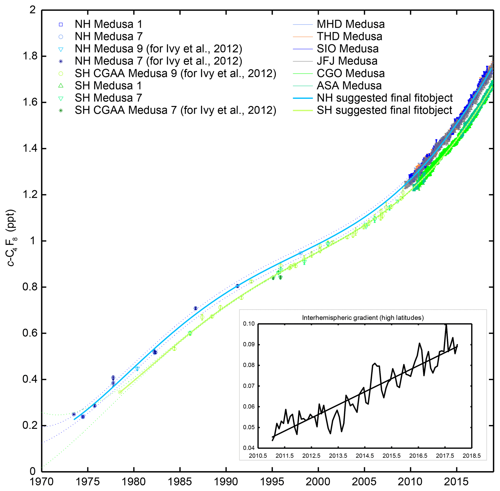
Figure 1 c-C₄F₈ mole fractions reconstructed from the late 1970s to 2018 from archived air samples and in situ measurements in both hemispheres. Cape Grim Air Archive (CGAA) and archived NH air samples are shown with symbols in shades of green and blue, respectively, reflecting different data subsets. For recent years, in situ measurements are shown as pollution removed monthly means for extratropical stations in the NH (MHD in light blue, THD in orange, SIO in darker blue, JFJ in grey) and in the SH (CGO in lighter green, ASA in pale green). Shown are the final data after an iterative filtering process described in the main text. The final suggested fits are shown as bold light green (SH) and bold light blue (NH) polynomial fits. Confidence bands (2σ) are shown as dotted lines. Results for the tropical stations, RPB and SMO, the Asian stations, GSN and SDZ, and the Arctic station, ZEP, are omitted here for clarity. For individual samples, error bars reflect measurement precisions. For monthly means, error bars represent standard deviations. The inset shows the interhemispheric gradient from in situ measurements at high latitudes (MHD, THD, SIO, and CGO) from 2011 to 2017.

2.3 Air extracted from firn

To augment the data set of in situ and archived air measurements, we measured c-C₄F₈ in samples from a subset of the firn sites described in Trudinger et al. (2016), namely NEEM08 in the NH and DSSW20K and SPO01 in the SH, plus one new site in the NH, Summit13, Greenland. We used the CSIRO firn model (Trudinger et al., 1997, 2013) to characterize the age of the air in these samples (detailed in Sect. 4.1). Here, we give a brief description of the firn sites. For a full description of the calibration of the CSIRO firn model for NEEM08, DSSW20K, and SPO01, see Trudinger et al. (2013), and for Summit13 see Fig. S1 in the Supplement.

NEEM08. Firn air was extracted from the EU borehole in July 2008 in northern Greenland, drilled near the North Greenland Eemian Ice Drilling Project (NEEM) deep ice core drilling site (77.45^∘ N, 51.06^∘ W) (Buizert et al., 2012). This site has a moderate snow accumulation rate of 199 kg m⁻² yr⁻¹.

Summit13. Firn air was collected in May 2013 at Summit, Greenland, from a borehole (72.66^∘ N, 38.58^∘ W) drilled 10 km NNW of Summit Station, Greenland. The US Firn Air system (Battle et al., 1996) was used to extract the air from 19 depth levels in the firn from the surface to just above 80.06 m (below this depth firn air can no longer be collected as the open channels in firn have closed off and formed discrete bubbles embedded in ice). The 3 in. borehole was drilled with the Eclipse Ice Drill (IDDO) and new rubber bladders (1∕8 in. thick) were fabricated (Greene Rubber Co., Woburn, MA) for use in this campaign. The 2.5 L glass flasks were filled at all depths for high-resolution measurements of gases performed by the National Oceanic and Atmospheric Administration (NOAA) (CO₂, CH₄, CO, N₂O, SF₆, H₂). Larger volume samples from preselected depth levels were filled in 35 L electro-polished SS tanks using a KNF Neuberger pump (with neoprene diaphragms). These samples were measured at SIO for c-C₄F₈ and other trace gases (including CH₄, N₂O, CFCs, HFCs, HCFCs, and SF₆). For quality control purposes, the sample line was measured on site for CO₂ and CH₄ by cavity ring-down spectroscopy (CRDS, Los Gatos Research, μ-GGA) and CO by a reducing compound photometer (Peak Labs, RCP1) prior to filling the flasks. Summit has a moderate snow accumulation rate of 211 kg m⁻² yr⁻¹. CSIRO firn model calculations for Summit use the density profile from Adolph and Albert (2014) and mean annual temperature and pressure of 241.75 K and 665 mbar. The diffusivity profile and related parameters were calibrated using the measurements of CO₂, CH₄, N₂O, SF₆, CFC-11, CFC-12, CFC-113, CH₃CCl₃, HFC-134a, HCFC-141b, and HCFC-142b described above. Firn model results for these tracers are shown in Fig. S1.

DSSW20K. Firn air was collected in January 1998 in eastern Antarctica (66.73^∘ S, 112.83^∘ E) from a borehole drilled 20 km west of the deep Dome Summit South (DSS) drill site near the summit of Law Dome (Smith et al., 2000; Sturrock et al., 2002; Trudinger et al., 2002). This site has a short firn column and a moderate snow accumulation rate of 150 kg m⁻² yr⁻¹.

SPO01. We only measured one sample collected in 2001 from 120 m from a borehole at the South Pole, Antarctica (90^∘ S, 119^∘ W) (Aydin et al., 2004; Sowers et al., 2005). This site has a deep firn column and a low snow accumulation rate of 75 kg m⁻² yr⁻¹, resulting in old firn air.

Firn air extracted from the DSSW20K, NEEM08, and SPO01 sites was measured at CSIRO in 2012 (Medusa 9), while Summit13 firn air was measured at SIO (Medusa 7), see Table 1. c-C₄F₈ firn measurement data are included in the data file listed in the Supplement. Other gases such as CH₄ and N₂O were measured as well.

2.4 Air samples collected over India and the Indian Ocean

Air samples were collected on board the UK FAAM (Facility for Airborne Atmospheric Measurements) BAe-146 aircraft during 11 flights conducted from 12 June to 9 July 2016 (9–28^∘ N, 72–86^∘ E) into 3 L pre-evacuated electropolished stainless steel flasks (SilcoCan, Restek) sealed with metal bellows valves (SS-BNVVCR-4, Swagelok). During the time it took to compress the air samples to 3.8 bar (30–60 s, depending on altitude) using a metal bellows pump (PWSC 28823-7, Senior Aerospace, USA), the aircraft traveled ∼7 km. Nine flights occurred over northern India and two over southern India and the Indian Ocean. In total, 176 flask samples were collected, with the majority (> 90 %) of these samples filled below 1.5 km altitude. The size of the subsamples analyzed with Medusa 21 at the University of Bristol was reduced to 1.75 L (from 2 L) and the sampling rate to 50 mL min⁻¹ (from 100 mL min⁻¹) to allow for triplicate analyses of each flask and to accommodate for the lower flask pressure. c-C₄F₈ measurements are reported on the SIO-14 calibration scale. Detection limits, blanks, and precisions were similar to those stated above. For further details, see Say et al. (2019).

3 Bottom-up emission inventories (UNFCCC, EDGAR, NIRs, WSC)

Emissions of compounds, such as c-C₄F₈, into the atmosphere are often estimated by so called “bottom-up” methods, which are based on information such as purchased, produced or imported amounts, industrial activities referred to as activity data, and estimated emission factors for each emissive process. Developed countries report annual emissions of GHG, including c-C₄F₈, to the UNFCCC using such bottom-up methods. However, these data are inherently not representative of total global emissions since developing countries do not have the same comprehensive UNFCCC reporting requirements, including countries such as South Korea, China, and Taiwan with sizable electronics and PTFE manufacturing capacities and thus with potentially significant c-C₄F₈ emissions. An additional complication is that several countries report unspecified mixes of PFCs or of PFCs and HFCs and other fluorinated compounds, making it difficult or impossible to estimate emissions of individual compounds, such as c-C₄F₈. In the Supplement, we gather available inventory information from submissions to UNFCCC, National Inventory Reports (NIRs), the Emissions Database for Global Atmospheric Research (EDGAR), the World Semiconductor Council (WSC), and the U.S. Environmental Protection Agency (EPA) in an effort to estimate contributions from unspecified mixes and countries not reporting to UNFCCC to compile a meaningful bottom-up inventory. Globally these add up to 10–30 t yr⁻¹ (0.01–0.03 Gg yr⁻¹) from 1990 to 1999, 30–40 t yr⁻¹ (0.03–0.04 Gg yr⁻¹) from 2000 to 2010, and 100–116 t yr⁻¹ (∼0.1 Gg yr⁻¹) from 2011 to 2014 (with a substantial fraction due to the US emissions from fluorocarbon production reported by the U.S. EPA). As has been found by Saito et al. (2010) and Oram et al. (2012), we show in Sect. 5.2 and 5.3 that measurement-based (top-down) global and most regional emissions are significantly larger than the compiled bottom-up c-C₄F₈ emission inventory information (see Fig. 5), analogous to what has been found for other PFCs (Mühle et al., 2010), reflecting the shortcomings of current emission reporting requirements and inventories.

4 Modeling studies

4.1 CSIRO firn model

The CSIRO firn model and its use in global inversion frameworks has been described in detail (Trudinger et al., 2013, 2016; Vollmer et al., 2016, 2018, 2019). Air samples taken far away from pollution sources represent the background atmospheric trace gas composition at that time. Once air enters the firn, vertical diffusion and other physical processes in the firn lead to mixing of air of different ages. Therefore, air extracted from firn must be described with an age distribution. We used the CSIRO firn model to describe the relationship between trace gas mole fractions measured in each extracted air sample from a given depth and the corresponding age distribution of high-latitude atmospheric mole fractions. The diffusion coefficient of c-C₄F₈ relative to that of CO₂ in air at 253 K used here was 0.47 with an estimated uncertainty of ∼10 %. This value was determined using Eq. (4) from Fuller et al. (1966) with Le Bas volume increments (e.g., Table 1.3.1, Mackay et al., 2006 and a multiplier for the Le Bas increments of 0.97, which minimizes the difference of calculated relative diffusion coefficients of a number of compounds from values measured by Matsunaga et al., 1993, 2002, 2005).

Figure 2 shows the measured depth profile of c-C₄F₈ (ppt) in air extracted from polar firn sites in the NH (Greenland) and the SH (Antarctica); for site details see Table 1. All samples showed c-C₄F₈ mole fractions above the detection limit. The firn reconstructed depth profiles are discussed in Sect. 4.3.1.

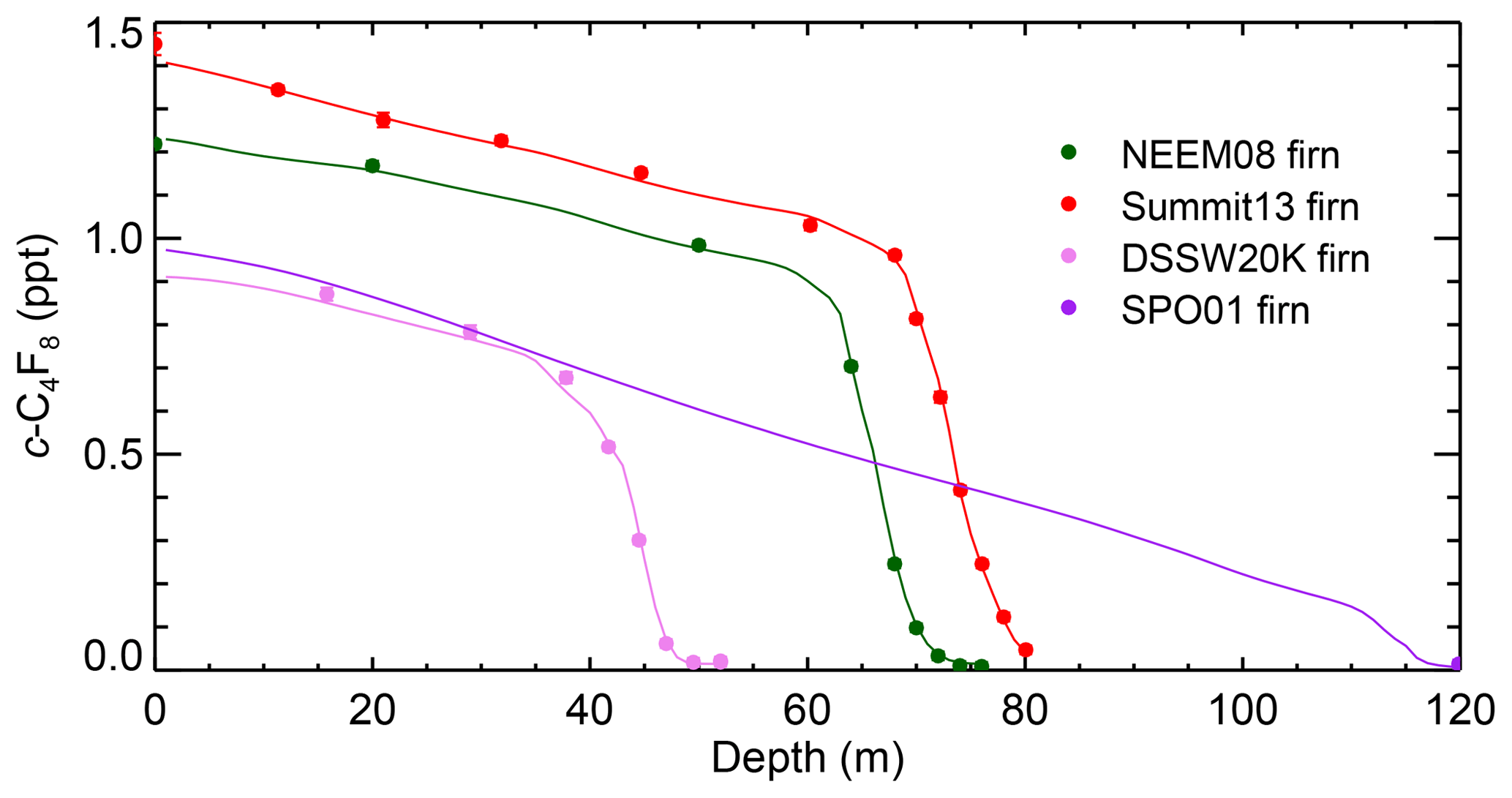
Figure 2 Depth profile of c-C₄F₈ measured dry-air molar mole fractions (parts per trillion, ppt) in air extracted from polar firn at NEEM08 (northern Greenland, dark green) and Summit13 (Greenland, red) in the NH and DSSW20K (eastern Antarctica, pink) and SPO01 (South Pole, purple) in the SH, together with the simulated depth profiles for each site (dark green, red, pink, and purple lines) that correspond to the emissions inferred by the CSIRO inversion. The modeled depth profiles for each site (solid lines) are based on the inversion of measurements from all firn sites, archive, and in situ data. Measurement precisions (1σ) are shown as error bars and are generally smaller than the plotting symbol.

4.2 AGAGE 12-box model of the global atmosphere

The AGAGE 12-box two-dimensional model (Cunnold et al., 1983, 1997; Rigby et al., 2013) describes the transport and loss of trace gases in the global atmosphere. The model divides the atmosphere into four latitudinal bands at 0^∘ and 30^∘ S and ^∘ N and three altitude bands at 500 and 200 hPa and calculates the mole fractions in each box. The AGAGE background sites (MHD, THD, RPB, SMO, and CGO; see Table 1) were historically chosen to represent the trace gas mole fractions in the four lower (tropospheric) model “boxes”. Model transport parameters were varied seasonally, but repeated annually. Given the very long atmospheric lifetime of c-C₄F₈ compared to the study period, the lifetime of c-C₄F₈ was assumed to be infinite in the model.

4.3 Global inversion methods

We used the AGAGE 12-box model in two different Bayesian inversions, denoted as the “CSIRO” and “Bristol” inversions, to estimate historic c-C₄F₈ emissions from our observations and to reconstruct historic abundances. Both inversions used in situ and archive data and the CSIRO inversion additionally used firn data. The observations need to be representative of clean background air at each sampling location. For in situ data, the AGAGE statistical method was used to remove pollution events and to calculate pollution-free monthly mean background air mole fractions for each AGAGE station (O'Doherty et al., 2001; Cunnold et al., 2002). As explained in Sect. 2.2, an iterative filtering algorithm starting out with all the archived air data and the pollution-free monthly means was then used to reject outliers for the extratropical SH and NH, mostly from the NH archive data. Due to the remoteness of the firn sample sites, we assumed background conditions without any filtering.

4.3.1 CSIRO inversion

The CSIRO inversion was developed to infer annual emissions at the global scale from firn, ice core, and atmospheric measurements (Sturrock et al., 2002; Trudinger et al., 2002, 2016). Green's functions from the CSIRO firn model were used to relate the measured air in the firn samples to air in the atmosphere in the past, and Green's functions from the AGAGE 12-box model were used to relate global emissions with a specified latitudinal distribution to mole fraction in the extratropical SH and NH. The inversion included constraints to avoid negative mole fractions, negative emissions, and unrealistic changes in emissions; these constraints were required due to the characteristics of inverting firn data and sparse archive data. The uncertainties in reconstructed mole fractions and inferred emissions were calculated using a bootstrap method that included the uncertainty in firn measurements, annual mean mole fraction (this uncertainty is temporally correlated; see Supplement in Vollmer et al., 2019), calibration scale (±2 %), and the firn model through the use of an ensemble of Green's functions corresponding to different firn model parameters including relative diffusivity (Trudinger et al., 2013, 2016; Vollmer et al., 2016).

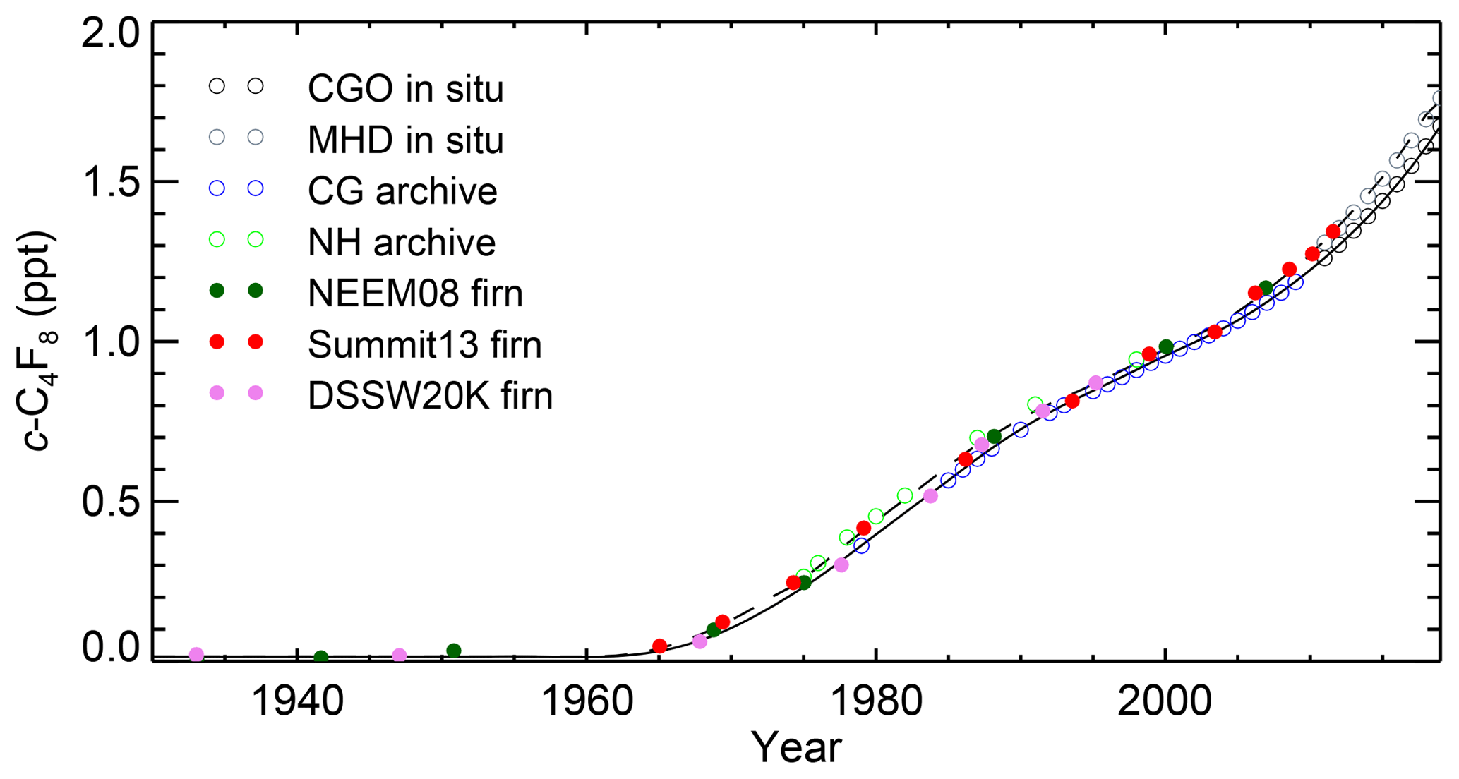
Figure 3 Historic atmospheric c-C₄F₈ mole fractions reconstructed for the extratropical Northern Hemisphere and Southern Hemisphere from air extracted from polar firn (full circles, NEEM08 in dark green, Summit13 in red, DSSW20K in pink, against mean or effective ages; SPO01 with mean age of ∼1890 is not shown), annual values from spline fits to Cape Grim Air Archive (CG archive, open blue circles) and in situ measurements at Cape Grim (CGO, open black circles), archived air samples (NH archive, open green circles), and in situ measurements at Mace Head (MHD, open grey circles). Also shown are reconstructed abundances based on optimized emissions determined by the CSIRO inversion for the extratropical SH (black line) and NH (dashed black line).

Figure 3 shows the data that were used in the CSIRO inversion: annual values based on 10-year smoothing spline fits (i.e., 50 % attenuation at periods of 10 years) to monthly means of pollution-free in situ measurements at the AGAGE background sites CGO (SH) and MHD (NH), annual values based on 10-year smoothing spline fits to measurements of the CGAA and archived NH air samples, and air extracted from polar firn in both hemispheres. Annual means from the spline were only used in the inversion when there were pollution-free archive or in situ measurements around that time. Figure 3 also shows the final reconstructed abundances for the extratropical SH (solid black line) and NH (dashed black line) based on the optimized emissions. The measured mole fractions in firn air are plotted against their effective atmospheric ages if that age is after 1965, where the effective ages are calculated using the reconstructed history of atmospheric mole fractions determined by the CSIRO inversion (Trudinger et al., 2002). Before 1965, the growth rate in the atmosphere was small and uncertain; this makes it difficult to determine effective ages, so the earlier firn measurements are plotted against their mean ages (see also Fig. S7). Firn depth profiles for each firn site corresponding to the CSIRO inversion results are shown in Fig. 2 (solid lines) and they typically agree with the measurements within precisions (1σ, shown as error bars).

Overall, the abundances reconstructed with the CSIRO inversion agree very well with the measurement data (see also Fig. S2). In Fig. S3, we show the effect of excluding different sites from the inversion on reconstructed emissions and mixing ratios and the sensitivity of the inversion to the relative diffusion coefficient of c-C₄F₈.

It should be pointed out that the deepest NEEM08 firn air sample for the NH showed slightly lower mole fractions (0.0085 ppt) than the deepest DSSW20K samples for the SH (0.021 and 0.0185 ppt), although the mean ages are similar (1930s). The same applies to the second deepest NEEM08 (0.0105 ppt) and DSSW20K (0.018 ppt) samples (1940s), which is unexpected for a long-lived anthropogenic compound predominantly emitted in the NH. While the differences seem significant within the nominal precisions (0–0.0014 ppt) achieved for these firn samples measured only one to two times, they are not significant within typical precisions achieved for archive samples (∼0.01–0.02 ppt), which are typically measured three or more times and these data are just at or below the typical detection limits of 0.01–0.03 ppt. Based on the order in which the firn samples were measured and the absence of detectable blanks, it seems unlikely that a small blank, memory, calibration, or measurement problem could have caused this small discrepancy. The early part of the reconstructed record, with near-zero mole fractions, is also most susceptible to small uncertainties in the calibrated diffusivity profiles versus depth for all sites used in the firn model, uncertainties in the firn model structure (e.g., physical properties being invariant of time), or uncertainties in the diffusivity of different tracers relative to each other. Thus, there are a number of possible reasons for the higher mixing ratio in the SH firn data at this time, and we do not interpret this as evidence of higher mole fraction in the SH in the 1930s or 1950s.

4.3.2 Bristol inversion

The Bristol inversion was used to estimate annual fluxes of c-C₄F₈ using archive and in situ observations only (Rigby et al., 2011, 2014; Vollmer et al., 2018). A priori, it was assumed that emissions were similar from year to year such that the a priori year-to-year emission growth rate was assumed to be zero with an uncertainty of 200 t yr⁻² (0.2 Gg yr⁻², 1σ), approximately twice the bottom-up estimate in Sect. 3. The derived emission uncertainties include contributions from the measurement repeatability, the calibration scale uncertainty, and the model–measurement representation error (Rigby et al., 2014). Furthermore, because some archive air samples exhibit substantial short-timescale (< 1 year) variations that are unlikely to represent real changes in the background atmosphere (Fig. 11), the minimum uncertainty was set to the maximum deviation of the archive air samples from the smooth curve in Fig. 11 (0.03 ppt). Model representation errors were estimated as the variability of the pollution-free monthly baseline means determined by the AGAGE pollution algorithm (O'Doherty et al., 2001; Cunnold et al., 2002) from the high-frequency in situ data at each station for each given month. For periods without in situ data, the representation error was assumed to be equal to the average baseline variability from in situ data in the same latitudinal band scaled by the measured c-C₄F₈ abundance. The calibration scale propagation uncertainty is estimated based on propagation uncertainties of the c-C₄F₈ calibration scale from primary gravimetric standards to secondary standards within the “R1” relative calibration framework used in AGAGE and on propagation uncertainties from the R1 framework to the standards used to measure individual samples. Figure 4 shows that there is good agreement between the archived air samples (Sect. 2.2) and the pollution-free monthly mean in situ data from the AGAGE background sites (MHD and THD, RPB, SMO, and CGO) used in the Bristol inversion and the reconstructed mole fractions for the four latitudinal bands which these samples represent (see also Fig. S4).

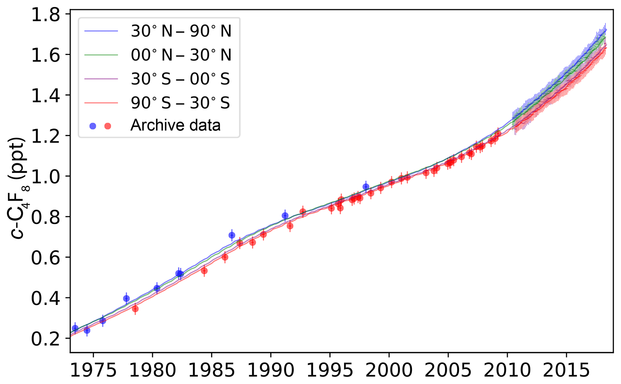
Figure 4 Historic c-C₄F₈ mole fractions from archive samples in both hemispheres (filled circles) and pollution-free monthly mean in situ data from AGAGE background sites (MHD and THD in blue, RPB in green, SMO in purple, and CGO in green vertical bars; bar size represents variability of monthly means) are shown together with the Bristol inversion results for the four latitudinal bands represented by these background sites (30–90, 0–30^∘ N, 0–30, and 30–90^∘ S, solid lines of same color).

4.4 Regional model and inversion study using NAME-HB for eastern Asia

To investigate regional emissions in eastern Asia (20–50^∘ N and 110–160^∘ E) from our observations we used an inversion method based on Bayesian inference. We estimated annual mean emissions, assuming that emissions are constant in both space and magnitude during each calendar year. Here, the inversion used observations from the Gosan station as this site was operated with relatively few interruptions from October 2010 to the end of 2017, with best data coverage from 2011 to 2015. These observations were binned into 12 hourly averages. The inversion method requires an atmospheric transport model to derive the sensitivity of the observations to a surface emission field. We used the Lagrangian NAME (Numerical Atmospheric dispersion Modelling Environment) model from the UK Met Office (Jones et al., 2007), driven by meteorology from the Met Office Unified Model (Walters et al., 2014). The sensitivity was derived by releasing 20 000 hypothetical air parcels per hour of measurement from Gosan station, which were transported backwards in time for up to 30 d. The model recorded the time and location that air parcels interacted with the surface (below 40 m above ground level at a spatial resolution of 0.352^∘ by 0.234^∘), and these data were used to form an aggregated 30 d sensitivity or “footprint” map for each hour of measurement. In addition, the model recorded the time and location that air parcels left the domain boundaries to provide the sensitivity to the boundary conditions. The footprint maps, generated over the domain 5^∘ S–74^∘ N and 55–192^∘ E and up to 19 km, were aggregated into 12 h averages.

We used a trans-dimensional hierarchical Bayesian method (NAME-HB) with a Metropolis–Hastings Markov chain Monte Carlo (MCMC) algorithm (Metropolis et al., 1953; Hastings, 1970) to solve the inverse problem. This allowed spatial emission estimates of c-C₄F₈ to be derived, whilst considering the uncertainties in the model, measurements, and a priori information and, importantly, the uncertainty in these uncertainties. Bayesian methods require a priori knowledge, here the emissions and boundary conditions. As little information on eastern Asia's c-C₄F₈ emissions (see Sect. 3) was available, we based our mean a priori emissions on those estimated by Saito et al. (2010). We spread their emissions for each reported country uniformly over the area of each country, rather than use population density (as in Saito et al., 2010) as that is not likely a good proxy of c-C₄F₈ emissions. We also spread 0.11 Gg yr⁻¹ of emissions over the rest of the domain where the footprint was calculated. The value of 0.11 Gg yr⁻¹ is an approximate scaling of the global total emissions based on population in this outer domain, i.e., the remainder of the domain not defined as eastern Asia. While we do not report emission estimates outside of eastern Asia due to large posterior uncertainties, they are still estimated in the inversion as they are useful when modeling the emissions in eastern Asia and their uncertainties that we do report. We assigned a large uncertainty to these a priori emissions (Table S1), which were governed by a lognormal distribution, so that they were uninformative and the observations dominated the estimation. We set a priori boundary conditions to be the mean background mole fractions measured at MHD on each vertical boundary (N, E, W, S) of the NAME domain. Offsets to the boundary conditions on each boundary were estimated in the inversion on a monthly basis.

The hierarchical nature of the inversion method means that hyper-parameters were also incorporated to include uncertainties in the NAME sensitivities, which are described by a multivariate normal distribution (see Ganesan et al., 2014). The reversible jump, or trans-dimensional, aspect of the inversion means that the underlying resolution at which the emissions are estimated is itself explored during inference (Lunt et al., 2016). Table S1 shows the a priori probability distributions assigned to the emissions and boundary condition scaling factors, model uncertainty, and the underlying grid. The posterior emission estimates and their uncertainties were governed by exploring the spaces of each of these parameters and hyper-parameters. The sensitivity of the emissions generally decreases with distance from the measurement site, which leads to increased uncertainty in the inversion, in both the spatial distribution of emissions and their overall magnitude. The further away emissions occur, the more likely the regional inversion method will allocate these emissions to a general diffuse region, rather than identify individual c-C₄F₈ point sources.

4.5 Regional model and inversion study using InTEM for western Europe

To investigate regional emissions in western Europe (36–66^∘ N and −14–31^∘ E) we used InTEM, an inversion framework (Arnold et al., 2018) based on the NAME Lagrangian transport model (Jones et al., 2007), together with observations from MHD, Tacolneston (TAC), Jungfraujoch (JFJ), and Monte Cimone (CMN). A priori estimates were considered unknown (see Sect. 3 and the Supplement) and therefore set to a uniform distribution of 0.2 Gg yr⁻¹ over the whole land area within the inversion domain with an uncertainty of 0–0.62 Gg yr⁻¹. Observational uncertainty was time varying and estimated as the variability of the observations in a 6 h moving window plus the measurement repeatability determined from repeat measurements of the on-site calibration standards. Model uncertainty was estimated every 2 h as the larger of the median of all pollution events at each station in a year or 16.5 % of the magnitude of the pollution event. A temporal correlation of 12 h was assumed in the model uncertainty at each station. An analytical solution was found that minimized the residual between the model and the observations and the difference between the posterior and the a priori flux estimate, balanced by the uncertainties of both. The baseline was estimated in the inversion following Arnold et al. (2018). The variable resolution of the inversion grid was calculated and refined within InTEM based on the magnitude of the footprint and emissions from each grid box. The inversions were run 24 times per year, each time with a randomly generated subsample (90 %) of the available observations from each station (10 % removed in 5 d blocks), to further explore the uncertainty. Emissions and uncertainties were averaged across the 24 individual inversions thereby assuming 100 % correlation between uncertainties in these separate inversions. We performed 1-year inversions covering the period 2013–2017.

4.6 Regional model and inversion study using NAME-HB for India

To investigate regional emissions from the Indian subcontinent from the samples taken on board a research aircraft in June and July 2016 (see Sect. 2.4) we used the NAME-HB inversion method described in Sect. 4.4 and Table S1. Here, the domain spanned from 6 to 48^∘ N and from 55 to 109^∘ E with an altitude up to 19 km and emissions were estimated as the mean over the 2-month period. As with eastern Asia and western Europe studies, the sensitivity of the atmospheric measurements to surface emissions was derived using the NAME model. Back-trajectories were simulated for each minute of each flight path for up to 30 d backward in time. To account for the motion of the aircraft, hypothetical air parcels were released from a cuboid whose dimensions were defined as the change in latitude, longitude, and altitude of the aircraft during each 1 min period, at a release rate of 1000 air parcels min⁻¹. Wherever possible, samples were collected during periods of level flight, to minimize the altitude component of the release volume. India's a priori emissions were set to 18 % of global c-C₄F₈ emissions (from Sect. 5.2), equal to India's fraction of the global population, but uniformly distributed over India. A large uncertainty was assigned (Table S1 in the Supplement) to reflect the lack of information on India's current c-C₄F₈ emissions. A priori vertical boundary conditions were assigned using background mole fractions from MHD (N, E, and W) and CGO (S). Offsets to these boundary conditions were estimated in the inversion. Due to the limited number of samples taken on board the aircraft, the regional inversion for the Indian subcontinent may have more difficulty identifying individual point sources (see Sect. 4.4), which may also not be emitting at all times. We report only emissions for northern and central India (NCI) as the inversion has low sensitivity over southern India and Sri Lanka and the northwestern edge of the domain, and no sensitivity beyond the Himalayas (see Fig. S5). Sensitivity tests indicate that c-C₄F₈ emissions determined for NCI are insensitive to the choice of a priori emissions (see Fig. S6).

4.7 Pollution events at Zeppelin station

The Zeppelin (ZEP) station is located in a clean Arctic environment and receives air masses representative mostly of the Arctic background. Nevertheless, 10 cases of enhanced c-C₄F₈ mole fractions were observed with the arrival of air masses from Eurasia. To trace the origin of these events, we used 3-hourly 50 d backward simulations for a passive tracer with version 10 of the Lagrangian particle dispersion model FLEXPART (Stohl et al., 2005). The model was driven with operational meteorological analyses of the European Centre for Medium Range Weather Forecasts (ECMWF, https://www.ecmwf.int/, last access: 10 February 2019). The model set-up was similar to that typically used for inversion studies (Stohl et al., 2009), but the number of events observed at the station was too small for a sensible regional inversion. Instead, we inserted unit emission sources (∼1 kg s⁻¹) at two facilities in Russia producing PTFE and halogenated chemicals including c-C₄F₈ (HaloPolymer, Kirovo-Chepetsk, Kirov Oblast and Galogen Open Joint-Stock Company, Perm), one or both of which we suspect to be responsible for the observed enhancements. We then scaled the modeled c-C₄F₈ mole fractions based on these two unit sources to the observed enhancements to estimate the source strength required to explain the observations. The two sources are quite close to each other and thus very much correlated so it was impossible to quantify the influence of each source individually, but it turned out that each source required about the same flux to produce a similar good match with the observations.

5 Results and discussion

5.1 Atmospheric histories of c-C₄F₈ in both hemispheres

Figure 1 shows the atmospheric histories of c-C₄F₈ in the extratropical NH and SH determined from several sets of archive measurements and pollution filtered data from six in situ measurement stations. As detailed in Sect. 2.2, the data shown have gone through an iterative filtering process which mostly removed outliers from the NH record. The pollution-free monthly mean in situ data for the four extratropical NH stations shown here and ZEP agree within precisions, although JFJ data tend to be at the lower range since early 2015 for unknown reasons. The two extratropical SH stations CGO and ASA also agree well with each other. Mole fractions measured in both hemispheres show a clear and consistent interhemispheric gradient reflecting the high precision of the measurements and indicating that emissions of c-C₄F₈ predominantly occur in the NH. These data form a consistent atmospheric record of c-C₄F₈ from the late 1970s to 2017 in both hemispheres, albeit with very sparse data for the NH before in situ measurements started at JFJ and at other NH stations. The inset in Fig. 1 shows that the interhemispheric gradient, based on in situ measurements at high-latitude stations in the NH (MHD, THD, SIO) and SH (CGO) has been rising from ∼0.05 ppt in 2011 to ∼0.09 ppt in 2017, which suggests increasing, predominantly NH, emissions.

To augment our c-C₄F₈ data set and to extend our reconstruction further backwards in time, we measured air samples extracted at several firn sites from both hemispheres and interpreted the data with the CSIRO global inversion framework. The CSIRO inversion (see Sect. 4.3.1) yields the atmospheric history of c-C₄F₈ starting in 1900 until present, although abundances are essentially not different from zero (< 0.02 ppt) until the early 1960s (Fig. 3). Average global c-C₄F₈ mole fractions from the CSIRO inversion reached 0.45 ppt in 1980, 0.74 ppt in 1990, 0.97 ppt in 2000, 1.29 ppt in 2010, and 1.66 ppt in 2017. The Bristol inversion (see Sect. 4.3.2) does not incorporate firn data; still, atmospheric histories of the two inversions are generally in good agreement (see Fig. S7).

The CSIRO inversion reconstructs that the global rise rate of c-C₄F₈ accelerated from near zero before the late 1960s to ∼0.03–0.04 ppt yr⁻¹ in the mid-1970s to late 1980s, after which the rise rate slowed to ∼0.02 ppt yr⁻¹ in the early 1990s to mid-2000s. It increased again in the early 2000s and reached ∼0.07 ppt yr⁻¹ in 2017.

Compared to Oram et al. (2012), our work extends the SH record from 2008 until present and, arguably, from 1978 back to 1900. Furthermore, it adds the full NH record. SH mole fractions reconstructed by Oram et al. (2012) are very similar in 1978 and 1990, but ∼0.06 ppt lower in the mid-1980s (∼11 %) and the late 1990s to late 2000s (∼5 %; see Fig. S8). Although the stated precision in Oram et al. (2012) of 0.8 % (∼0.01 ppt at 1.2 ppt) is similar to the 0.01–0.02 ppt achieved here, the resulting precisions of the CGAA measurements achieved here are significantly improved. For example, the noise in the CGAA reconstruction by Oram et al. (2012) is about as large as the interhemispheric gradient determined here (see Fig. S8). The estimated accuracy of the SIO-14 c-C₄F₈ calibration scale of ∼2 % also compares favorably to previous calibration scale uncertainties.

5.2 Global c-C₄F₈ emissions

Global c-C₄F₈ emissions (Fig. 5 and Supplement) started to increase in the early 1960s (CSIRO inversion) from near zero to ∼1.2 Gg yr⁻¹ in the late 1970s to the late 1980s. The Bristol inversion initially reconstructs lower emissions, but the differences are within the estimated uncertainties for the reconstructed histories (see Fig. 5). Afterwards, emissions determined by both inversions declined to ∼0.8 Gg yr⁻¹ in the mid-1990s to early 2000s. After that emissions kept increasing, reaching ∼2.2 Gg yr⁻¹ in 2017. Both inversions reconstruct emissions which are significantly larger than available bottom-up inventory information (see Sect. 3 and the Supplement), reflecting the shortcomings of the current UNFCCC reporting requirements and bottom-up inventories.

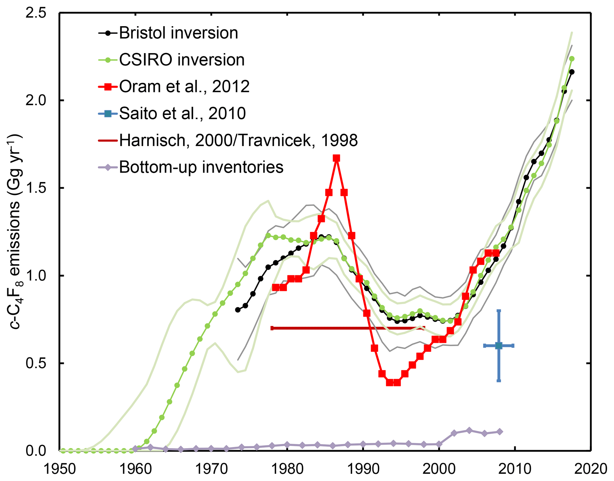
Figure 5 Global c-C₄F₈ emissions reconstructed by the CSIRO inversion (green dots and line, light green 2σ uncertainty bands) from 1950 and by the Bristol inversion (black dots and line, grey 1σ uncertainty bands) from the early 1970s to present. In situ and archive data are used in both inversions, while firn air data are only used in the CSIRO inversion. Emission estimates by Oram et al. (2012) (red), Saito et al. (2010) (blue), Harnisch (2000)/Travnicek (1998) (brown), and from available bottom-up inventory information (grey) are shown for comparison.

Emissions presented by Oram et al. (2012) agree very well from 2001 to 2007 with our results and on average also from 1978 to 2001, although they show larger variability. Global emissions roughly estimated by Harnisch (2000) based on measurements by Travnicek (1998) of ∼0.7 Gg yr⁻¹ from 1978 to 1997 are 30 % lower than our estimate of 1.01±0.10 Gg yr⁻¹. Saito et al. (2010) estimated global emissions of 0.6±0.2 Gg yr⁻¹ from January 2006 to September 2009, about half of our 1.16±0.09 Gg yr⁻¹ estimate. This difference is likely due to slowly changing c-C₄F₈ mole fractions in calibration tanks used by NIES (Takuya Saito, personal communication, 2018), which would significantly affect the background rise rate and thus global emissions, but would have had less influence on the regional emissions estimated by Saito et al. (2010) as these are mostly dependent on the magnitude of the much larger pollution events above background.

Global emissions of c-C₄F₈ have clearly not leveled off at 2005–2008 levels as had been suggested by Oram et al. (2012), but kept rising. In contrast, emissions of other minor PFCs, C₂F₆ and C₃F₈, have decreased since the early 2000s and stabilized in recent years (Trudinger et al., 2016), reflecting that emission sources and/or use patterns of c-C₄F₈ are different from those of the other minor PFCs. Weighted by GWP₁₀₀ (100-year timescale) estimated 2017 emissions of c-C₄F₈, C₃F₈, C₂F₆, and CF₄ were 0.021, 0.005, 0.022, and 0.083 billion metric tons (tonnes) of CO₂-eq., respectively (see Fig. S9). c-C₄F₈ CO₂-eq. emissions have been larger than those of C₃F₈ since 2004 and, assuming continued growth, will also surpass C₂F₆ emissions within a year or two, so that c-C₄F₈ will become the second most important PFC emitted into the global atmosphere in terms of CO₂-eq. emissions. In the next section, we will investigate regional emissions of c-C₄F₈ to gain a better understanding how individual regions and sources may contribute to the global emissions.

5.3 Regional c-C₄F₈ emission studies

5.3.1 Emissions from eastern Asia

Within the AGAGE network, the two stations in eastern Asia, Gosan (GSN) and Shangdianzi (SDZ), show by far the most frequent and most pronounced pollution events of up to ∼14 ppt above NH background, indicating significant regional emissions (see Fig. S10). Therefore, we use a regional inverse method (NAME-HB) to infer the emissions in this region (20–50^∘ N and 110–160^∘ E; see Sect. 4.4). We focus on the observations from GSN as this site was operated with relatively few interruptions from June 2010 to the end of 2017 and had almost full coverage for each year from 2011 to 2015. Significantly longer data gaps exist for SDZ, which would have made interpretation of inversion results more difficult. The sensitivity of the inversion generally decreases with distance to the receptor station, resulting in relatively low sensitivity for emissions from western China, eastern Japan, and parts of Taiwan (the cumulative footprint map for 2010–2017 is shown in Fig. S11). Therefore, we report in Table 2 and Fig. 6 estimated emissions for eastern China, western Japan, South Korea, North Korea, and Taiwan. c-C₄F₈ emissions in this eastern Asian domain increased from 0.36±0.07 Gg yr⁻¹ in 2010 to 0.73±0.13 Gg yr⁻¹ in 2016 and 2017 and were dominated by emissions from eastern China. The a priori emissions for eastern China of 0.185 Gg yr⁻¹ are based on the Saito et al. (2010) estimate for all of China for November 2007 to September 2009, but the inversion suggests emissions that are ∼62 % higher in 2010 and more than triple in 2017. Note that if we were to sum up emissions for all regions of China, including those where the inversion has low sensitivity, total emissions would be another ∼50 %–75 % higher. In contrast, the EDGAR 4.2 emission inventory, the only available bottom-up information (see Sect. 3 and the Supplement), suggests no significant emissions from China.

Table 2 Regional c-C₄F₈ emissions derived for eastern Asia from Gosan measurements (NAME-HB inversion) and comparison to global emissions (Gg yr⁻¹, kt yr⁻¹).

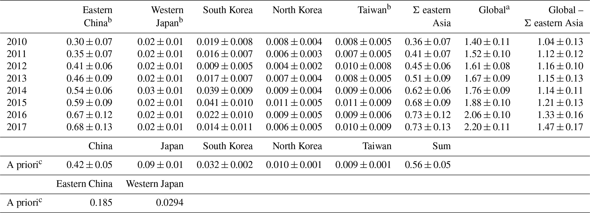
^a Global emissions are the average of the emissions determined by the CSIRO and the Bristol inversion in this work. ^b Eastern China contains the provinces Anhui, Beijing, Hebei, Henan, Jiangsu, Liaoning, Shandong, Shanghai, Shanxi, Tianjin, and Zhejiang. Western Japan contains the prefectures Chugoku, Kansai, Shikoku, and Okawa and Kyushu. Due to the lower sensitivities of the inversion in western China, eastern Japan, and parts of Taiwan, where potential source industries are located, we cannot exclude further emissions in these regions and therefore total emissions are probably larger. ^c Saito et al. (2010) emission estimates based on atmospheric measurements from November 2007 to September 2009 were used as a priori information and were spread for each country uniformly over the area of each country. The resulting a priori estimates for eastern China and western Japan are additionally listed for comparison with the inversion results for these regions. Gosan measurements started in June 2010 with most complete coverages from 2011 to 2015.

For western Japan we find emissions of ∼0.02 Gg yr⁻¹ (no trend), ∼30 % lower than the a priori emissions (from Saito et al. 2010; see Sect. 4.4). While total country emissions are likely higher, the available bottom-up information (see Sect. 3 and Supplement) suggests an order of magnitude lower emissions for all of Japan. For South Korea, the inversion adjusts emissions down to 0.01–0.02 Gg yr⁻¹ in most years and up to ∼0.04 Gg yr⁻¹ in 2014 and 2015. Except perhaps for 2012 and 2017, emissions from South Korea are significantly higher than the 0.003–0.008 Gg yr⁻¹ suggested by the available bottom-up information. Emissions from Taiwan show no trend and are relatively small with ∼0.01 Gg yr⁻¹, which is ∼50 % of ∼0.02 Gg yr⁻¹ indicated by the Taiwanese NIR, though it should be noted that the inversion has relatively low sensitivities for some parts of Taiwan (see Fig. S11). Overall, emissions from western Japan, South Korea, and Taiwan are small, despite their large semiconductor industries (see also Fig. 7), suggesting that this industry sector is not a major emitter of c-C₄F₈. Emissions from North Korea are also small.

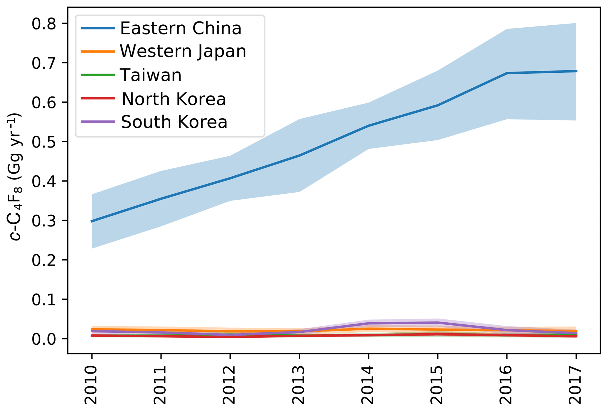
Figure 6 c-C₄F₈ emissions in eastern Asia as determined by the NAME-HB regional inversion of measurements at the Gosan station, Jeju Island, South Korea, are dominated by emissions from China (blue). Emissions from western Japan (orange) and South Korea (violet) are much smaller; the latter show a small maximum in 2014 and 2015. Emissions from Taiwan (green) and North Korea (red) are also small. Shadings represent uncertainty bands of emissions.

Combined regional c-C₄F₈ emissions doubled from 2010 to 2016, driven by Chinese emissions. They represent 31±4 % of global emissions (2010–2017), while eastern China's emissions represent 28±4 %. The difference between global and eastern Asian emissions remained relatively consistent, ranging from ∼1.04 Gg yr⁻¹ in 2010 to 1.47 Gg yr⁻¹ in 2017 with an average of 1.20±0.14 Gg yr⁻¹ from 2010 to 2017 and 1.15±0.03 Gg yr⁻¹ from 2011 to 2015, the years with the best data coverage at GSN and thus highest confidence in the results. This means that the increase in global emissions is essentially explained by the increase in eastern Asian emissions, i.e., mostly from China, but also that significant emissions of ∼1.16 Gg yr⁻¹ exist outside of the investigated region (a fraction of which may stem from industries located in parts of China and perhaps Japan where the inversion has low sensitivity).

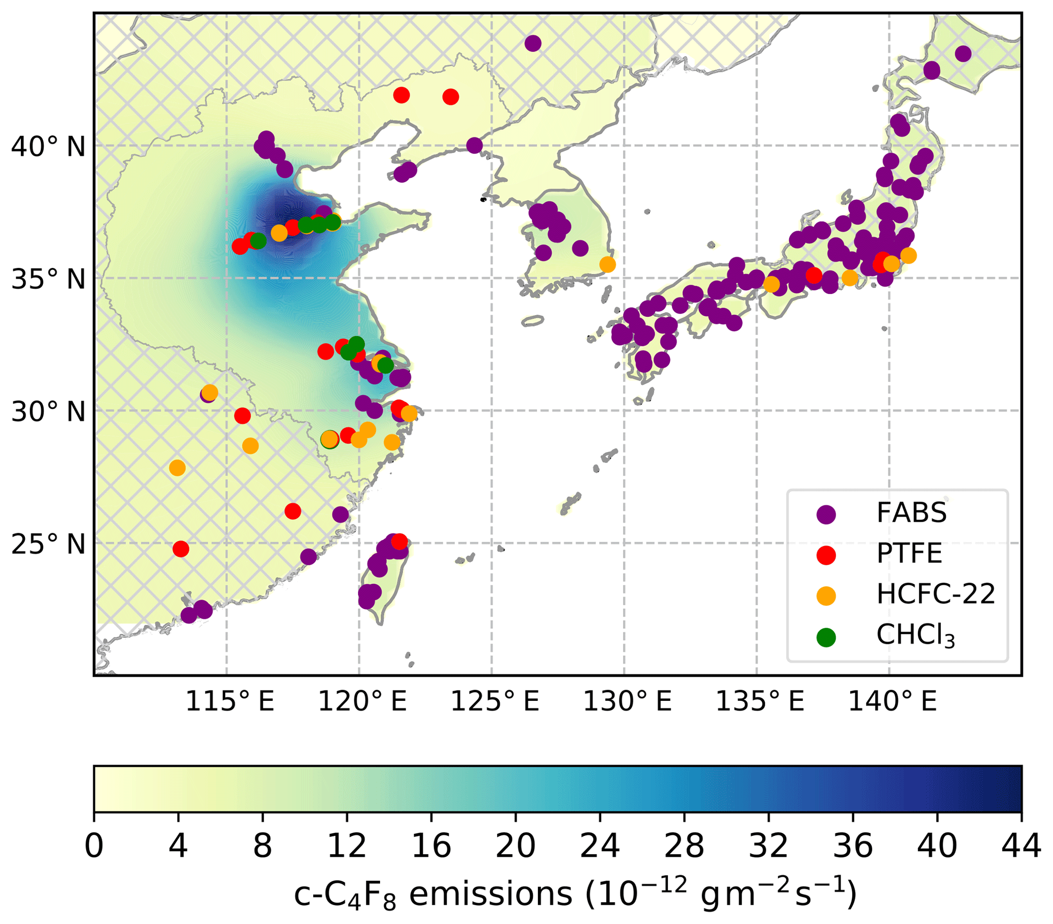
Figure 7 Mean c-C₄F₈ emission strength (shades of green and blue, 10⁻¹² g m⁻² s⁻¹) in eastern Asia from 2010 to 2017 determined by the NAME-HB inversion from measurements at the Gosan station, Jeju Island, South Korea. The hatching indicates areas for which emissions are not reported due to relatively low sensitivities of the inversion. Emissions predominantly occur in the densely industrialized Shandong, Tianjin, and parts of Henan and Hebei provinces south/southwest of Beijing as well as in Shanghai and neighboring provinces Jiangsu (to the north), Anhui (to the west), and Zhejiang (to the south) of the Yangtze River Delta region. Shown are industries with potential c-C₄F₈ emissions: semiconductor fabrication plants (FABS, purple dots, https://en.wikipedia.org/wiki/List_of_semiconductor_fabrication_plants, last access: 3 December 2018; http://www.10stripe.com/featured/map/semiconductor-fabs.php, last access: 3 December 2018; and other sources) and TFE–HFP–PTFE–FEP production facilities (PTFE, red dots, https://www.qianzhan.com/analyst/detail/220/170629-c33a2ca7.html, last access: 12 December 2018; and other sources). HCFC-22 (orange dots) and chloroform (CHCl₃, green dots) production facilities are shown as the TFE and HFP monomers needed to produce PTFE and FEP fluoropolymers are produced via pyrolysis of HCFC-22 and c-C₄F₈ is an intermediate/by-product in this process, while HCFC-22 is manufactured from CHCl₃.

Figure 7 shows that from 2010 to 2017 emissions in eastern China occur from the highly industrialized provinces Shandong, Tianjin, and parts of Henan and Hebei (south/southwest of Beijing) as well as from Shanghai and neighboring Jiangsu (to the north), Anhui (to the west), and Zhejiang (to the south) in the Yangtze River Delta region. Also shown are locations of potential industrial c-C₄F₈ point sources. For South Korea, western Japan and Taiwan, semiconductor fabrication plants do not seem to be dominant c-C₄F₈ emitters as they are not co-located with large c-C₄F₈ emissions (though the inversion has low sensitivity for eastern Japan, where many more semiconductor fabrication plants (FABS) and several PTFE and HCFC-22 plants are located; hence emissions from this region cannot be analyzed).

In China, the picture is less clear than in South Korea, Japan, and Taiwan, as several semiconductor fabrication plants in the Yangtze River Delta region are co-located with strong c-C₄F₈ emissions, while those near Beijing are not. Many of the potential production facilities of TFE and HFP monomers and PTFE and FEP polymers are co-located with areas where strong c-C₄F₈ emissions occur. This is consistent with information from the second largest producer of PTFE in China that they do not recover c-C₄F₈ by-product, but do emit c-C₄F₈ to the atmosphere (Jianxin Hu, personal communication, 2018). Still, the two facilities northeast of Beijing do not seem to emit c-C₄F₈, perhaps reflecting that some producers minimize c-C₄F₈ emissions, e.g., to increase yield or to use c-C₄F₈ for other purposes, such as for the semiconductor industry. Several facilities are also located in provinces for which the inversion has low sensitivity. Most HCFC-22 production facilities are not co-located with strong c-C₄F₈ emissions, while CHCl₃ production facilities tend to be in areas with c-C₄F₈ emissions. This may reflect that CHCl₃ production has shifted from use as a feedstock to produce HCFC-22 for dispersive applications (refrigeration or foam blowing), where no c-C₄F₈ emissions occur, to production of TFE–HFP–PTFE–FEP via HCFC-22 pyrolysis, where c-C₄F₈ by-product emissions occur, perhaps at the same or close-by facilities. This would be consistent with the start of the HCFC phase-out for dispersive applications in developing countries mandated by the Montreal Protocol on Substances that Deplete the Ozone Layer. Then again, CHCl₃ has other uses, e.g., as solvent (Tsai, 2017), without any potential c-C₄F₈ emissions.

Note that at one or both of the PTFE production facilities in Zhejiang province (Juhua Group Corporation) HFO-1234yf has been produced since 2016, using a process which starts out with the same chemistry needed for PTFE–FEP production, that is the pyrolysis of HCFC-22 to TFE and HFP, with c-C₄F₈ as a potential by-product (see Supplement).

There is no strong correlation between c-C₄F₈ emission distribution and population density, e.g., emissions from Henan and Hebei provinces are significantly lower than those from Shandong despite similar total population, which may indicate that combustion of fluoropolymers in waste incineration facilities (Morisaki, 1978; Kannan et al., 2005; van der Walt et al., 2008; Ji et al., 2016; Bezuidenhoudt et al., 2017) is not a dominant source of c-C₄F₈ emissions.

If c-C₄F₈ emissions in eastern Asia are predominantly associated with TFE–HFP–PTFE–FEP production via the pyrolysis of HCFC-22, c-C₄F₈ emissions may co-occur with small emissions of TFE and HFP. HFC-23 emissions may also co-occur as HCFC-22 is produced from CHCl₃ and HFC-23 is a by-product that in developing countries is probably again vented to the atmosphere since the UNFCCC Clean Development Mechanism (CDM) funding to avoid HFC-23 emissions has expired (Simmonds et al., 2018; Say et al., 2019). While the global atmospheric lifetime of TFE is only ∼2 d, the lifetime of HFP is ∼6 d (Acerboni et al., 2001), so that HFP may be detectable near strong emission sources and serve as a sensitive marker for regional TFE–HFP–PTFE–FEP production. After adding HFP to the measurements in late 2018, we find that HFP pollution events at SDZ always coincide with c-C₄F₈ and HFC-23 pollution events (see Fig. S12 and its caption in the Supplement). HFP pollution events at GSN are much weaker, reflecting the short atmospheric lifetime and the more distant source region, but they also coincide with c-C₄F₈ and HFC-23 pollution events. At both sites, however, c-C₄F₈ pollution events also coincide with enhancements of other anthropogenic compounds which may just point to generally polluted air in the region, so it is difficult to draw definitive conclusions. Still it is clear that HFP is emitted in eastern Asia, likely in China, and HFP as well as c-C₄F₈ emissions can be explained by PTFE–FEP production. Measurements of HFP at SIO and ASA confirm that it is virtually absent (≤0.01 ppt) from the global background atmosphere even in urban environments.

Overall, the strong c-C₄F₈ emissions in eastern China and their source regions are consistent with our hypothesis of emissions from TFE–HFP–PTFE–FEP production facilities due to little or no recovery or abatement of c-C₄F₈ by-product and the significant fraction of global PTFE production (53 %–67 % in 2015) occurring in China (see Table S3).

5.3.2 Emissions from northwestern Europe

Outside of eastern Asia, the TAC station in East Anglia, UK, shows by far the most frequent and most pronounced c-C₄F₈ pollution events of any AGAGE station, with a few reaching ∼5 to 10 ppt above NH background, indicating close-by emissions. Data from the TAC, MHD, JFJ, and CMN stations and the InTEM regional inverse method (see Sect. 4.5) were used to estimate emissions from northwestern Europe (42 to 59^∘ N and −11 to 15^∘ E) based on the areas of highest sensitivity to the observations (see Fig. S13). Compared to eastern Asia, we find only small emissions of 0.026±0.013 Gg yr⁻¹ (Ireland, UK, France, Germany, Belgium, the Netherlands, Luxemburg, and Denmark, 2013–2017) without any significant temporal trend, corresponding to only ∼1 % of global emissions, despite an estimated 14 % of global PTFE production in 2015 (see Table S3). The mean distribution of emissions is shown in Fig. 8. Similar to eastern Asia, many identified semiconductor FABS in Europe are not co-located with c-C₄F₈ emission hot spots, while several FABS in northern France, the UK, Ireland, and the Netherlands seem to be co-located. Producers of PTFE and FEP and facility locations in Europe were determined from company websites (3M/Dyneon, AGC/Asahi Glass, Arkema, Chemours/DuPont, Saint-Gobain, Solvay) and the European Pollutant Release and Transfer Register (https://prtr.eea.europa.eu/#/home, last access: 16 January 2019), but it is very difficult to determine at which of the many facilities PTFE or FEP is actually produced and thus where c-C₄F₈ may be emitted. It seems that several facilities in the Netherlands, Belgium, the UK, France, and Italy which likely produce PTFE are co-located with identified c-C₄F₈ emission hot spots (Fig. 8). Still, many mismatches exist, reflecting the uncertainties in determining the exact facility locations, the relatively small emission strength, and uncertainties of the inversion. As in eastern Asia, there seems to be no correlation with population density, which suggests that waste incineration of fluoropolymers is not a dominant c-C₄F₈ source here either. The inversion is broadly consistent with emissions from TFE–HFP–PTFE–FEP production and FABS, but emissions from other industrial sources may also play a role. While emissions of 0.026±0.013 Gg yr⁻¹ are relatively small, it is noteworthy that UNFCCC reports suggest much smaller c-C₄F₈ emissions (0.0007 Gg yr⁻¹, UNFCCC, 2013–2014 and 0.0017 Gg yr⁻¹, bottom-up emission inventories, Sect. 3, 2013–2014).

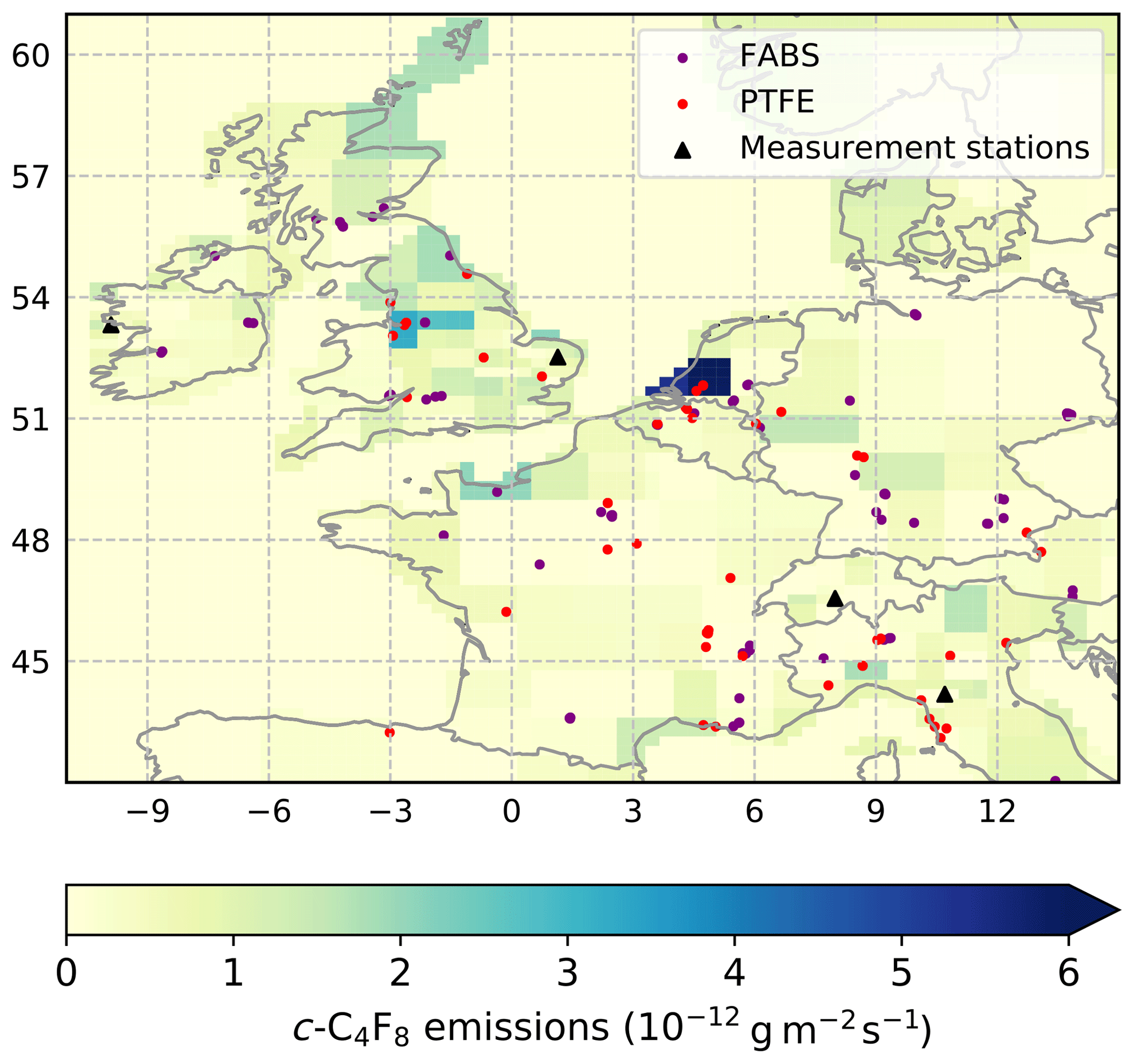
Figure 8 Mean c-C₄F₈ emission strength (shades of green and blue, 10⁻¹² g m⁻² s⁻¹) in northwestern Europe (42 to 59^∘ N and −11 to 15^∘ E) from 2013 to 2017 determined by the InTEM inversion from measurements at four sites (Mace Head, Ireland, Tacolneston, United Kingdom, Jungfraujoch, Switzerland, and Monte Cimone, Italy, black triangles). Also shown are potential industrial emitters of c-C₄F₈. Locations of potential TFE/HFP/PTFE/FEP production facilities (red dots) are based on company websites (3M, Chemours, Daikin, DuPont, Saint-Gobain, and Solvay) and are much less certain than the corresponding location information for eastern Asia. Also shown are semiconductor fabrication plants (purple dots, https://en.wikipedia.org/wiki/List_of_semiconductor_fabrication_plants, last access: 3 December 2018; http://www.10stripe.com/featured/map/semiconductor-fabs.php, last access: 3 December 2018; and other sources).

5.3.3 Emissions from southeastern Australia

Other urban locations of the AGAGE network, such as SIO, USA, and ASA, Australia, show much smaller pollution events above global background (up to ∼2.5 ppt) than those seen at TAC, suggesting even lower emissions. Still, the few pollution events at ASA and even CGO are interesting as production of PFCs in Australia has never been recorded. CFC-11, CFC-12, and HCFC-22 were manufactured starting in 1962 at two facilities in Sydney, but production ceased in 1995 and trace gas emissions from Sydney are rarely if ever observable at CGO or ASA. Without any currently known fluorocarbon production, any c-C₄F₈ pollution events observed at CGO or ASA should not be due to fugitive emissions. c-C₄F₈ imports to Australia are ∼4 to 50 kg yr⁻¹ (2011–2015), likely for minor refrigeration uses. In contrast, small but identifiable c-C₄F₈ pollution episodes at CGO suggest Melbourne emissions of ∼2 t yr⁻¹ (0.002 Gg yr⁻¹) in 2016 (down from ∼5 t yr⁻¹ in 2009, inter-species correlation method, ISC; see Fraser et al., 2014; Dunse et al., 2018). Scaled by population to Australia (for lack of a better proxy), emissions from 2009 to 2016 could be ∼10–25 t yr⁻¹ (0.01–0.025 Gg yr⁻¹), 2–3 orders of magnitude higher than import data suggest. Since early 2017, HFP has been measured at ASA (see Fig. S12 caption). Occasionally, small HFP pollution events, which are often, but not always, associated with c-C₄F₈ pollution events, may point to small-scale production of TFE–HFP–PTFE–FEP in Melbourne or perhaps these small emissions stem from incineration of waste-containing fluoropolymers. Another possible explanation could be that more c-C₄F₈ is imported in products for minor applications than identified in import data due to inadequate labeling. On a global scale, estimated Australian c-C₄F₈ emissions of ∼0.015 Gg yr⁻¹ are small, ∼0.7 % of global emissions. PFC (CF₄, C₂F₆) pollution episodes at Cape Grim and Aspendale due to PFC emissions from southeastern Australian aluminum smelters (Portland and Pt. Henry, Victoria, and Bell Bay, Tasmania) do not show any evidence of c-C₄F₈ emissions (Fraser et al., 2013; CSIRO unpublished data).

5.3.4 Emissions from under-sampled regions such as the US, India, and Russia

The AGAGE network does not closely monitor large areas of the globe where c-C₄F₈ emissions may occur. For example, many semiconductor FABS are located in the western, southern, and eastern US and chemical facilities located in the southern and eastern US are estimated to account for ∼10 % of global PTFE production in 2015, while facilities in India and Russia are estimated to account for ∼8 % and ∼6 %, respectively (see Tables S3 and S4). The two AGAGE stations in California are only able to capture a fraction of these emissions due to predominant westerly winds and therefore we cannot estimate c-C₄F₈ emissions from the continental US. If PTFE production facilities in the US are operated as in NW Europe, emissions should be similarly small. If facilities in India and Russia are operated as in China, emissions could be significant as well. In the case of Russia this seems likely as the original technology for fluoropolymer production in China apparently stems from Russia (Buznik, 2009).

5.3.5 Emissions from India

Say et al. (2019) recently presented measurements from an aircraft campaign in June and July 2016 (see Sect. 2.4) over the Indian subcontinent to determine emissions of ODS and HFCs. Here we use their c-C₄F₈ measurements and the NAME-HB inversion (see Sect. 4.6) and estimate emissions of 0.14 (0.09–0.20) Gg yr⁻¹ for northern and central India (NCI). Data are only available for two months in 2016, but seasonality in industrial emissions of c-C₄F₈ is not expected. Given the limitations of the inversion method to identify distant point sources from a relatively small number of samples (see Sect. 4.4 and 4.6), the posterior emission distribution (Fig. 9) is consistent with emissions from facilities producing PTFE. Several of the HCFC-22 production facilities are co-located or very close to these PTFE-producing facilities, suggesting that a fraction of HCFC-22 is pyrolyzed to produce monomers for PTFE and FEP. Two HCFC-22 production facilities are outside of areas with strong c-C₄F₈ emissions, possibly because these two sites focus on production of HCFC-22 for dispersive applications (refrigeration or foam blowing), where no c-C₄F₈ emissions occur. The single FAB in India we are aware of is not co-located with significant c-C₄F₈ emissions. As in eastern Asia and northwestern Europe, there is no apparent correlation of c-C₄F₈ emissions with population density. Emissions predominantly occur outside of the Indo-Gangetic plain, the most densely populated region of India, which excludes potential sources that scale with population. Instead the inversion allocates emissions in a much less densely populated region in which multiple likely industrial point sources for c-C₄F₈ are located. The derived emissions account for 6.8 (4.4–9.7) % of global c-C₄F₈ emissions in 2016, in comparison to the estimated ∼8 % of 2015 global PTFE production capacity (see Table S3). While we cannot categorically exclude an unknown industrial source, these results are consistent with the chemistry of TFE–HFP–PTFE–FEP production as a dominant c-C₄F₈ emission source. Note that one of the facilities in western India (Navin Fluorine International, Surat, Gujarat) is known to also produce HFO-1234yf since 2016, using a process which starts out with the same chemistry, that is the pyrolysis of HCFC-22 to TFE and HFP, with c-C₄F₈ as potential by-product (see Supplement). All known Indian PTFE manufacturers are located within the NCI domain; hence the estimated emissions are likely to be roughly representative of India's national total, though further atmospheric measurements would be required to confirm this.

Figure 9 Mean c-C₄F₈ emission strength (shades of green and blue, 10⁻¹⁴ g m⁻² s⁻¹) over the Indian subcontinent for June and July 2016 determined by the NAME-HB inversion based on air samples taken on board UK's FAAM (Facility for Airborne Atmospheric Measurements) BAe-146 research aircraft. Also shown are the locations of one semiconductor fabrication plant (FAB, purple dot) and several potential TFE–HFP–PTFE–FEP production facilities (PTFE, red dots, Solvay/CYTEC, Hindustan Fluorocarbons, and Gujarat Fluorochemicals facilities) as potential c-C₄F₈ sources. HCFC-22 (orange dots) production facilities are also shown as the TFE and HFP monomers needed to produce PTFE and FEP fluoropolymers are produced via pyrolysis of HCFC-22 and c-C₄F₈ is an intermediate/by-product in this process. The outline of the northern and central India (NCI) model domain is shown as a pink line.

5.3.6 Emissions from facilities in Russia

Measurements at the ZEP site in remote Svalbard show 10 small c-C₄F₈ pollution events above the NH background of up to ∼0.4 ppt. FLEXPART backward simulations could trace some of these events to two facilities in Russia which produce PTFE and halogenated chemicals including c-C₄F₈ itself (HaloPolymer, Kirovo-Chepetsk, Kirov Oblast, and Galogen Open Joint-Stock Company, Perm). Figure S14 shows the FLEXPART footprint emission sensitivity map for the largest observed c-C₄F₈ enhancement on 19 November 2016, suggesting direct transport from the two sites. The emission sensitivity maps indicate that for six of the 10 observed pollution events the air had clearly passed over one or both of these two sources, even though the timing of the observed events was often not well matched by the model, which was sometimes off by up to about half a day. While this is not surprising given the large distance between the source and the receptor, it means that the two sources could not be clearly separated, especially since the FLEXPART emission sensitivity often also covered both sites for the same arrival times at ZEP. Assuming a unit emission at those two locations and scaling the resulting simulated mole fractions at ZEP to the observed enhancements above background, we estimated the emission strength for the two sites together for each event (see Sect. 4.7). Five of the 10 pollution events could be approximately reproduced by this method and required a flux of 0.18±0.06 Gg yr⁻¹, while the sixth event required ∼0.54 Gg yr⁻¹. Averaged for all six events 0.24±0.15 Gg yr⁻¹ would be required. Either of these fluxes would be significant, representing 9±3 %, 26 %, and 12±7 % of global emissions, respectively, compared to ∼6 % of estimated global PTFE production in Russia. The uncertainty of this estimate is large because only a few events were observed and not all of them were reproduced equally well by FLEXPART. Similar to eastern Asia, the largest c-C₄F₈ pollution event also showed enhancements of HFC-23, pointing to TFE–HFP–PTFE chemistry as a source (see Fig. S15), but other halogenated compounds were also elevated.

6 Summary and conclusions

We determine the atmospheric histories of c-C₄F₈ (PFC-318, perfluorocyclobutane) in both hemispheres based on measurements of archived, in situ, and firn air samples in conjunction with the CSIRO firn model, the AGAGE 12-box model, and two global inversion frameworks. Compared to previous studies, our work extends the Southern Hemisphere record from 1978 back to 1900 and from 2008 until 2017 and adds a Northern Hemisphere record, all reported with improved precisions for air archive measurements (∼1 %–2 %) and a lower uncertainty (2 %) of the SIO-14 gravimetric calibration scale. We find global c-C₄F₈ atmospheric mole fractions near zero (< 0.02 ppt) from 1900 until the early 1960s, after which they rose sharply, reaching 0.45 ppt in 1980, 0.74 ppt in 1990, 0.97 ppt in 2000, 1.29 ppt in 2010, and 1.66 ppt in 2017. Global c-C₄F₈ emissions started to increase in the 1960s from near zero to $\sim \mathrm{1.2}\pm \mathrm{0.1}$ (1σ) Gg yr⁻¹ in the late 1970s to the late 1980s. After this, emissions declined to $\sim \mathrm{0.77}\pm \mathrm{0.03}$ Gg yr⁻¹ in the mid-1990s to early 2000s. After this emissions again increased, reaching ∼ 2.20±0.05 Gg yr⁻¹ in 2017. These global emissions are significantly larger than what can be compiled from available bottom-up inventory information (70±17 times, 1990–1996, 29±5 times, 1997–2010, 15±1 times, 2011–2014).

Using the NAME-HB regional inverse method and observations at Gosan station we find that emissions from eastern Asia rose from ∼0.36 Gg yr⁻¹ in 2010 to ∼0.73 Gg yr⁻¹ in 2016 and 2017, representing 31±4 % of global emissions, predominantly from eastern China. Strong c-C₄F₈ emissions are found from heavily industrialized provinces south/southwest of Beijing and near the Yangtze River Delta. In contrast, emissions from western Japan, South Korea, and Taiwan are small, suggesting that their large semiconductor industries are not major c-C₄F₈ emitters. While we cannot categorically exclude emissions from other industrial sources, overall, the strong c-C₄F₈ emissions in eastern China and their spatial pattern are roughly consistent with emissions from production of TFE–HFP–PTFE–FEP and other fluorochemicals. A significant fraction of global PTFE production (53 %–67 % in 2015) occurs in China and, as indicated by the second largest producer of PTFE in China, the c-C₄F₈ by-product from the underlying HCFC-22 pyrolysis process is not recovered or abated, but rather emitted to the atmosphere.

Based on samples collected over the Indian subcontinent in mid-2016, we determine emissions of 0.14 (0.09–0.20) Gg yr⁻¹ c-C₄F₈ from northern and central India (NCI), ∼6.8 (4.4–9.7) % of global emissions. Within the limitations of the inversion, the determined emission map is also roughly consistent with emissions from TFE–HFP–PTFE–FEP production.

Using the InTEM regional inverse method and measurements at four western European stations, we only find small NW European emissions of $\sim \mathrm{0.026}\pm \mathrm{0.013}$ Gg yr⁻¹ c-C₄F₈ from 2013 to 2017 (∼1 % of global emissions), in contrast to an estimate of 14 % of global PTFE production capacity in 2015. The inversion also points to facilities which may produce PTFE and FEP and semiconductor fabrication plants though the picture is less clear.

No obvious correlation between population density and c-C₄F₈ emissions is found in eastern Asia, NCI, and NW Europe, indicating that incineration of waste-containing fluoropolymers is not a major source of c-C₄F₈.

Based on data from two Australian stations and an inter-species correlation method, Australian c-C₄F₈ emissions are estimated to be small, perhaps ∼0.7 % of global c-C₄F₈ emissions. We find no evidence for c-C₄F₈ production from three large aluminum smelters in SE Australia.

Based on a few c-C₄F₈ pollution events observed at Zeppelin station and a rough FLEXPART analysis, we estimate that emissions from two Russian facilities known to produce PTFE and halocarbons including c-C₄F₈ itself could be $\sim \mathrm{0.24}\pm \mathrm{0.15}$ Gg yr⁻¹. While this could represent a significant fraction of global emissions (possibly ranging from 5 % to 26 %), uncertainties are very large.

In summary, for the year 2016, we find global c-C₄F₈ emissions of 2.06±0.10 Gg yr⁻¹, with 0.73±0.12 Gg yr⁻¹ from parts of eastern Asia (36 % of the global total), 0.14 (0.09–0.20) Gg yr⁻¹ from northern and central India (6.8 %), $\sim \mathrm{0.026}\pm \mathrm{0.013}$ Gg yr⁻¹ from northwestern Europe (∼1 %), and ∼0.015 Gg yr⁻¹ from Australia (∼ 0.7 %).

Current monitoring capabilities of the AGAGE network leave large areas with potential c-C₄F₈ emission sources un- or under-monitored, e.g., most of the US, India, Russia, western China, and eastern Japan, where various semiconductor facilities and fluorochemical and fluoropolymer production plants are located.

While many possible uses and emission sources of c-C₄F₈ are found in the literature and though we cannot categorically exclude unknown industrial sources, the start of significant c-C₄F₈ emissions around the 1960s may well be related to the initial synthesis of PTFE in 1938 with commercial production of PTFE (Teflon) by DuPont commencing in 1947 (Gangal and Brothers, 2015) via pyrolysis of HCFC-22, with c-C₄F₈ as a by-product/intermediate. It seems unlikely that process control or abatement to minimize c-C₄F₈ by-production was in place in the early decades of PTFE production and c-C₄F₈ by-product was probably emitted to the atmosphere, explaining the steep increase in global emissions reconstructed here. With the advent of UNFCCC by-product reporting requirements in the 1990s, concern about climate change and product stewardship, abatement, and perhaps collection of c-C₄F₈ for use in the semiconductor industry where it can be easily abated, it is conceivable that fugitive c-C₄F₈ emissions in developed countries (UNFCCC Annex 1) overall were reduced, explaining the observed stabilization and reduction of global emissions in the 1980s and 1990s. Similar efforts to contain and destroy by-product emissions of fluorocarbons, e.g., HFCs, from the 1980s to the 2000s are documented in the Toxics Release Inventory (https://www.epa.gov/toxics-release-inventory-tri-program, last access: 5 February 2019) Program of the U.S. EPA and the European Pollutant Release and Transfer Register. Concurrently, production of PTFE in China increased rapidly, e.g., from 2000 to 2005 by ∼ 26 % yr⁻¹, followed by a slowdown to ∼14 % yr⁻¹ from 2005 to 2015 and perhaps ∼8 % yr⁻¹ from 2015 onward, reaching an estimated 53 %–67 % of global production in 2015 (see Tables S2, 3, and 4). Without any emission reduction requirements, it is conceivable that fugitive emissions of c-C₄F₈ from TFE–HFP–PTFE–FEP production in China, and other developing (UNFCC non-Annex 1) countries today dominate global emissions. The 2010 to 2016 rise in rates of eastern Chinese (eastern Asian) c-C₄F₈ emissions of ∼15 % yr⁻¹ (∼13 % yr⁻¹) determined here is compatible with these PTFE production increase rates of 14 to 8 % yr⁻¹ in China. Barring other developments, we predict that c-C₄F₈ emissions will continue to rise and that c-C₄F₈ will become the second most important PFC emitted to the global atmosphere in terms of CO₂-eq. emissions within a year or two. While the 2017 radiative forcing of c-C₄F₈ (∼0.52 mW m⁻²) is very small compared to that of CO₂, emissions of c-C₄F₈ and other perfluorinated compounds with similarly long lifetimes and high radiative efficiencies essentially permanently alter the radiative budget of Earth. The fact that significant emissions of ∼1.16 Gg yr⁻¹ of global emissions (56 %) exist outside of the monitored regions clearly shows that observational capabilities and reporting requirements need to be improved to understand global and country-wide emissions of PFCs and other synthetic greenhouse gases and ozone-depleting substances.