Machine learning for observation bias correction with application to dust storm data assimilation

Data assimilation algorithms rely on a basic assumption of an unbiased observation error. However, the presence of inconsistent measurements with nontrivial biases or inseparable baselines is unavoidable in practice. Assimilation analysis might diverge from reality since the data assimilation itself cannot distinguish whether the differences between model simulations and observations are due to the biased observations or model deficiencies. Unfortunately, modeling of observation biases or baselines which show strong spatiotemporal variability is a challenging task. In this study, we report how data-driven machine learning can be used to perform observation bias correction for data assimilation through a real application, which is the dust emission inversion using PM₁₀ observations.

PM₁₀ observations are considered unbiased; however, a bias correction is necessary if they are used as a proxy for dust during dust storms since they actually represent a sum of dust particles and non-dust aerosols. Two observation bias correction methods have been designed in order to use PM₁₀ measurements as proxy for the dust storm loads under severe dust conditions. The first one is the conventional chemistry transport model (CTM) that simulates life cycles of non-dust aerosols. The other one is the machine-learning model that describes the relations between the regular PM₁₀ and other air quality measurements. The latter is trained by learning using 2 years of historical samples. The machine-learning-based non-dust model is shown to be in better agreement with observations compared to the CTM. The dust emission inversion tests have been performed, through assimilating either the raw measurements or the bias-corrected dust observations using either the CTM or machine-learning model. The emission field, surface dust concentration, and forecast skill are evaluated. The worst case is when we directly assimilate the original observations. The forecasts driven by the a posteriori emission in this case even result in larger errors than the reference prediction. This shows the necessities of bias correction in data assimilation. The best results are obtained when using the machine-learning model for bias correction, with the existing measurements used more precisely and the resulting forecasts close to reality.

1 Introduction

For centuries, East Asia experienced regular dust storms in the springtime. Those dust events mainly originated from the dust source regions of the Gobi and Taklamakan deserts. Annually, thousands of metric tons of “yellow sands” are blown eastward over the densely populated areas in China, the Korean peninsula, and Japan by the prevailing winds. Dust storms can also carry irritating spores, bacteria, viruses, and persistent organic pollutants (WMO, 2017). In addition to affecting human health, the resulting low visibility can cause a severe disruption of transportation systems. For example, more than 1100 flights have been delayed/canceled in Beijing after the city was struck by a choking dust storm in early May 2017.

A large number of dust simulation models have been developed over the past decades (Wang et al., 2000; Gong et al., 2003; Liu et al., 2003). These chemistry transport models help to understand the life cycles of the dust storms, and are also used for dust forecasts and to aid early-warning systems. Apart from advances in simulation of dust storms, progress has also been made in the monitoring of dust or general aerosol loads. Field station networks are constructed to observe the in situ particulate matter (PM) levels over densely populated regions (Li et al., 2017a). Ground-based sun photometers, e.g., the global Aerosol Robotic Network (AERONET) (Cesnulyte et al., 2014), are widely used to monitor column-integrated aerosol profiles. Satellite onboard instruments such as the Moderate Resolution Imaging Spectroradiometer (MODIS) (Remer et al., 2005), Cloud-Aerosol Lidar and Infrared Pathfinder Satellite Observations (CALIPSO) (Sekiyama et al., 2010), and Advanced Himawari Imager/Himawari-8 (Yoshida et al., 2018) provide measurements of airborne particles with further wide coverages. These measurements could be used to calibrate the parametrization in dust simulation models and to evaluate their ability to forecast dust concentrations. Moreover, the observations could be combined with a dust modeling system through data assimilation to improve the forecast skills.

A wide variety of data assimilation techniques have been used with dust simulation models, including variational methods (Yumimoto et al., 2008; Niu et al., 2008; Gong and Zhang, 2008; Jin et al., 2018) and ensemble-based sequential methods (Lin et al., 2008; Sekiyama et al., 2010; Khade et al., 2013; Di Tomaso et al., 2017). In these systems, the available observations are used to either estimate the model states (dust concentrations) or reduce uncertainties in the emissions and/or other model parameters. Challenges for dust assimilations include development of more and more accurate dust simulations and use of new types of observations including vertical profiles from lidars and the latest satellite observations. A further challenge for any assimilation system is the proper definition of the observation and representation errors, as well as characterization of biases.

In general, the commonly used data assimilation schemes all rely on the basic assumption of an unbiased observation. In real applications, however, measurement biases are often unavoidable. In the presence of biases, it is impossible to determine whether a difference between a priori simulation and an observation is due to biased observations or model deficiencies. The biases might lead to assimilations that diverge from reality (Lorente-Plazas and Hacker, 2017). A well-known example of observation biases is in radiance observation assimilation systems in the presence of clouds (Eyre, 2016; Berry and Harlim, 2017). To avoid problems with these biases, up to 99 % of cloudy observed measurements are discarded, although they may also contain valuable information. If dust storms are coincident with clouds, it is also possible that in satellite retrieval algorithms clouds are mistaken for dust, leading to strong biases in the data to be assimilated (Jin et al., 2019).

Another example of where observation biases are important is when ground-based PM₁₀ measurements are assimilated in dust simulation models. Due to the high temporal resolution and the rather dense observation network, ground-based air quality observing networks have become a powerful source of measurements on dust aerosols. The records, mainly the PM₁₀ feature, were widely used to calibrate, assess, or estimate the dust model (Lin et al., 2008; Wang et al., 2008; Huneeus et al., 2011; Yumimoto et al., 2016; Benedetti et al., 2018). However, the observed PM₁₀ concentrations do not only consist of dust, but are actually the sum of the dust and other regular particles. The latter are emitted not only from anthropogenic activities such as industries, vehicles, and households, but also from natural sources such as wildfires and sea spray. In this paper we will simply refer to these particles as the non-dust fraction of the total PM₁₀. The concentrations of non-dust aerosols in urbanized areas could be substantial, reaching values up to 500 µg m⁻³ (Shao et al., 2018).

Although PM₁₀ observations include a nontrivial bias, the widespread availability still makes them useful in a dust storm assimilation system. During dust storm events, extreme high peaks of more than 1000–2000 µg m⁻³ PM₁₀ are recorded, which can be attributed mainly to dust. If these were assimilated directly in a dust simulation model, ignoring the fact that at least some part represents non-dust, the assimilation system would diverge to states that overestimate the dust load. In the case of less severe dust events, the dust analysis divergence would then become extremely critical.

However, modeling of observation biases is very challenging when they have strong spatial and temporal variabilities. Little progress has been made in bias correction of fully aerosol measurements for their use in dust storm data assimilation. Lin et al. (2008) selected only PM₁₀ observations for assimilation when at least one occurrence of dust clouds was reported by the local stations. In Jin et al. (2018), it was found that on sites with both PM₁₀ and PM_2.5 observations, only the PM₁₀ concentration increased during a dust episode, while the PM_2.5 concentrations were not affected and remained at a constant level. In addition, Xu et al. (2017) and Jin et al. (2018) suggested a strong correlation between PM_2.5 and non-dust PM₁₀. Therefore, a very simple non-dust PM₁₀ baseline removal (called observation bias correction) was proposed, in which the available PM_2.5 was used to approximate the non-dust PM₁₀ (or baseline) during a dust event by

$$\begin{array}{}\text{(1)}& {\text{PM}}_{\mathrm{10}}^{\text{non-dust}}=b+r\times {\text{PM}}_{\mathrm{2.5}},\end{array}$$

where b and r>1 are linear regression parameters based on a 24 h history of measurements before arrival of the dust storm.

The aforementioned methods either exclude a selection of the measurements, which may still contain useful information, or work under ideal circumstances only when a simple correlation R between PM₁₀ and PM_2.5 is valid. For instance, in the dust event studied in Jin et al. (2018) the application of Eq. (1) at many sites failed since R is weak. To have a quality-assured bias correction, Eq. (1) is performed only when the Pearson correlation coefficient ℛ>0.8. Consequently, measurements at around 45 % sites are rejected in that case. To fully exploit the dust information present in total PM observations, a more advanced method is needed. In this paper we proposed two methods, using either a conventional chemistry transport model or a machine-learning model.

A chemistry transport model (CTM) implements all available knowledge on emission, transport, deposition, and other physical processes in order to simulate concentrations of trace gases and, important here, aerosols. Daily air quality forecasts are often provided using such CTMs. A simulation model for dust storm events is usually just a CTM with all tracers removed except dust; by using the full CTM, an estimate of the non-dust part of the aerosol load could be made. In this study, the LOTOS-EUROS CTM is used to simulate the dust as well as the non-dust aerosol concentrations. If the non-dust model were perfect, the difference between simulation and observed PM₁₀ would be unbiased, and assimilation could be applied to the combined dust and non-dust concentrations. In the case of a dust storm event, it remains necessary to distinguish between the dust and non-dust part of the simulations since the two parts will have very different error characteristics. The dust part is quickly varying and has a large uncertainty, while the non-dust part is more smooth but very persistent in time and has a relatively small uncertainty. An assimilation system on the combined simulations should be able to handle these differences. However, the error attribution to their proper sources (dust and non-dust error) then becomes extremely critical as explained in Sect. 2.4. Since this paper focuses on dust during a severe event only, we will not explore the error characteristics of the non-dust part of the model. Therefore we will not apply an assimilation to the combined aerosol (dust and non-dust) model. Instead, the non-dust simulations will solely be used to remove the non-dust baseline from PM₁₀ observations.

Similar to the air quality forecast, the accuracy of a CTM for non-dust aerosols is hampered by lack of accurate input data. For example, the timely update of anthropogenic emission inventories is always a key issue for air quality forecasts. With ever-increasing complexity and resolution, CTMs are now becoming highly nonlinear and time-consuming. However, they may still not be able to identify explicit representations of the non-dust aerosol dynamics, especially regarding fine-scale processes.

In addition to conventional CTMs, we propose a new method for removing the non-dust part of the PM₁₀ observations, which is based on machine learning (ML). Data-driven methods have already been proven to be a powerful tool to provide air quality forecasts for horizons of a few days (e.g., Li et al., 2016, 2017b; Fan et al., 2017; Chen et al., 2018). Different from chemistry transport models, which simulate aerosol physical processes, machine-learning models describe mathematical relations of input–output and are trained by learning a large number of samples from historical records. Our machine-learning system used a neural network, namely long short-term memory (LSTM). The input is formed by air quality indices for a number of relevant tracers (PM_2.5, SO₂, NO₂, CO, and O₃), as well as meteorology data. The output of the system is an estimate of the non-dust PM₁₀ concentration. The input features are to a large extent independent of the dust storms, even the PM_2.5 concentrations as shown in Jin et al. (2018); observations of PM₁₀ are excluded since excessive dust loads are visible mainly in this component. Recent development and the availability of open-source machine-learning tools provide a good opportunity to estimate the air quality indices using a data-driven machine-learning model.

Whereas these are previous studies on dust storm data assimilation using various kinds of combined aerosol measurements, we are the first to investigate the necessities of bias correction for these fully aerosol observations in order to use them as “real” dust measurements in a dust storm assimilation system. The adding values of observation bias correction in dust emission inversion are explored through the ground-based PM₁₀ measurement assimilation. It can easily be used for other general applications, e.g., remote-sensing data assimilation. Our contributions are threefold. Firstly, we present and examine the conventional CTM for removing the non-dust part from PM₁₀ observations. Secondly, we design and examine a novel machine-learning-based bias correction which is data-driven and free of time-consuming numerical CTMs. Thirdly, we evaluate the two non-dust aerosol model simulations by comparing to the PM₁₀ measurements during regular periods (rare dust events involved); we evaluate dust emission fields, surface dust concentration simulation and forecast skills which are obtained by assimilating either the raw PM₁₀ data or bias-corrected measurements using either a CTM or machine-learning model.

The paper is organized as follows. A brief description of our dust simulation model (LOTOS-EUROS/dust) and the four-dimensional variational data assimilation method for emission inversion are presented in Sect. 2. The biased observation representing error and its influence on the assimilation system are also explained. The two bias correction methods, the non-dust aerosol regional chemistry transport model and a machine-learning model, are discussed and the bias simulation is evaluated in Sect. 3. Section 4 reports the assimilation results using the two bias correction methods, and evaluates the forecast skills using independent measurements. Section 5 discusses the necessities of observation bias correction in assimilation work and highlights our key contributions.

2 Dust storm data assimilation system

2.1 Dust model

The dust storm event studied in this paper took place in East Asia in April 2015, and has already been used as a test case for assimilation experiments in Jin et al. (2018). The LOTOS-EUROS/dust simulation model is used with configurations similar to those in our previous studies, which were configured on a domain from 15 to 50^∘ N and 70 to 140^∘ E, but with a higher model resolution of 0.25^∘. The model is driven by European Centre for Medium-Range Weather Forecasts (ECMWF) operational forecasts for horizons of 3–12 h. The dust load is described by five aerosol bins within a diameter range of 0.01 µm $<D_{\text{p}}<$ 10 µm. Physical processes included are emission, advection, diffusion, dry and wet deposition, and sedimentation. The dust emission scheme implemented in LOTOS-EUROS is mainly based on the formulation of horizontal saltation flux (Marticorena and Bergametti, 1995) and sandblasting efficiency (Shao et al., 1996). A terrain preference parameter F_ps was used in the dust emission in Jin et al. (2018). This geographic-dependent parameter was first introduced by Ginoux et al. (2001), and used to approximate the probability of having accumulated sediments that can be resuspended. In this work, F_ps is disabled since the preference factor was found to limit the emission rate in some regions where the fine-scale topographic feature is actually unknown. Snapshots of a reference simulation of the dust episode have been taken and are shown in Fig. 8a.

2.2 Observation network

The China Ministry of Environmental Protection (MEP) has commenced to release the hourly-average measurements of atmospheric constituents including PM_2.5, PM₁₀, CO, O₃, NO₂, and SO₂ since 2013. A huge number of ground stations measuring these air quality indices have been established in densely populated areas. At the present, the monitoring network has grown to 1500 field stations covering all of China as shown in Fig. 1.

Figure 1 The China MEP air quality monitoring network and the potential dust storm source region. LSTM-based non-dust PM₁₀ forecasts are performed only at stations with a blue dot (N=1351), while ones with black circles are skipped.

2.3 Reduced tangent linearization 4D-Var

The assimilation system, which will be used to combine bias-corrected PM₁₀ observations with simulations, is based on a reduced-tangent-linearization four-dimensional variational (4D-Var) data assimilation. The goal of a 4D-Var technique is to find the maximum likelihood estimation of a state vector, which is here the dust emission field f, given the available observations over a time window. A common approach is to use an incremental formulation, which aims to find the optimal emission deviation δf as the minimum of the cost function:

$$\begin{array}{}\text{(2)}& \begin{array}{rl}J\left(\mathit{\delta }\mathit{f}\right)=& {\displaystyle \frac{\mathrm{1}}{\mathrm{2}}}\mathit{\delta }\mathit{f}{\mathbf{B}}^{-\mathrm{1}}\mathit{\delta }\mathit{f}+{\displaystyle \frac{\mathrm{1}}{\mathrm{2}}}\sum _{i=\mathrm{1}}^k{\left({\mathbf{H}}_i{\mathbf{M}}_i\mathit{\delta }\mathit{f}+{\mathit{d}}_i\right)}^T\\ & {\mathbf{R}}_i^{-\mathrm{1}}\left({\mathbf{H}}_i{\mathbf{M}}_i\mathit{\delta }\mathit{f}+{\mathit{d}}_i\right)\end{array},\end{array}$$

where k is the number of time steps within the assimilation window. The vector δf denotes a perturbation of the emissions with respect to the background one. For an observation time i, the innovation vector (length m_i) is defined as the difference between the simulations and observations:

$$\begin{array}{}\text{(3)}& {\mathit{d}}_i={\mathcal{H}}_i\left({\mathcal{M}}_i\right(\mathit{f}\left)\right)-{\mathit{y}}_i,\end{array}$$

where ℳ_i denotes the LOTOS-EUROS/dust transport model, ℋ_i is the operator that converts state variables into observation space, and y_i is the vector with dust observations at this time step i. The operators H_i and M_i denote linearizations of ℋ_i and ℳ_i around the reference emission vector f_b. Following Jin et al. (2018), the errors in dust emission field were assumed to be only caused by the uncertainty in the friction velocity threshold in the dust windblown parametrization, and similar assumptions on the uncertainty are used to build an emission error covariance B. The friction velocity threshold is perturbed with a spatially varying multiplicative factor β. β is configured with a mean of 1 and a standard deviation of 0.1. In addition, an exponential profile of distance-based spatial correlation is posed on β values (Jin et al., 2018). The observation error term is weighted by an observation error covariance R, for which the individual elements will be described in Sect. 4.1.

To reduce the computational cost in calculating the tangent linear model M_i, a reduced-tangent-linearized 4D-Var (Jin et al., 2018, 2019) is used. The simplified method is based on proper orthogonal decomposition (POD) of the background covariance B, which efficiently carries out model reduction by identifying the few most energetic modes:

$$\begin{array}{}\text{(4)}& \begin{array}{rl}& \mathbf{B}={\mathbf{UU}}^T\approx \stackrel{\mathrm{̃}}{\mathbf{U}}{\stackrel{\mathrm{̃}}{\mathbf{U}}}^T\\ & \mathit{\delta }\mathit{f}\approx \stackrel{\mathrm{̃}}{\mathbf{U}}\mathit{\delta }\mathit{w}\end{array},\end{array}$$

where $\mathbf{U}\in {\mathbf{R}}^{P\times P}$ is the background emission covariance square root, with P the size of the emission field of O(10⁴) elements, while $\stackrel{\mathrm{̃}}{\mathbf{U}}\in {\mathbf{R}}^{P\times p}$ is the truncation of U based on POD, with p the reduced rank size of O(10²). The vector δw∈R^p stores the transformed control variables.

The cost function of the reduced-tangent-linearization 4D-Var is formulated as

$$\begin{array}{}\text{(5)}& \begin{array}{rl}J\left(\mathit{\delta }\mathit{w}\right)=& {\displaystyle \frac{\mathrm{1}}{\mathrm{2}}}\mathit{\delta }{\mathit{w}}^T\mathit{\delta }\mathit{w}+{\displaystyle \frac{\mathrm{1}}{\mathrm{2}}}\sum _{i=\mathrm{1}}^k{\left({\mathbf{H}}_i{\stackrel{\mathrm{̃}}{\mathbf{M}}}_i\stackrel{\mathrm{̃}}{\mathbf{U}}\mathit{\delta }\mathit{w}+{\mathit{d}}_i\right)}^T\\ & {\mathbf{R}}_i^{-\mathrm{1}}\left({\mathbf{H}}_i{\stackrel{\mathrm{̃}}{\mathbf{M}}}_i\stackrel{\mathrm{̃}}{\mathbf{U}}\mathit{\delta }\mathit{w}+{\mathit{d}}_i\right)\end{array},\end{array}$$

where ${\stackrel{\mathrm{̃}}{\mathbf{M}}}_i$ denotes the reduced tangent linear model with a rank p, which is approximated using the perturbation method. More details about the reduced-tangent-linearization 4D-Var algorithm can be found in Jin et al. (2018).

2.4 Biased observation representing error

In real applications, the observations inevitably have biases which cannot be attributed to the model simulation, as follows:

$$\begin{array}{}\text{(6)}& {\mathit{y}}_i={\mathcal{H}}_i\left({\mathcal{M}}_i\right(\mathit{f}\left)\right)+{\mathit{b}}_i+{\mathit{\sigma }}_i,\end{array}$$

where σ_i is the vector of Gaussian-distributed observation errors which have zero means and a known covariance matrix R_i, and b_i denotes the vector of observation bias. In our application, the vector y_i contains the observed PM₁₀ concentrations, while the aerosols released in the local anthropogenic activities and other non-dust-related processes are referred to as b_i. Note that the PM₁₀ measurements themselves might also contain “native” biases due to incorrect sensor reading or systematic errors. However, this part of the bias in the PM₁₀ observations is unknown and not considered in this study.

In the course of data assimilation, it is impossible to determine whether the departures (d_i) of the prior simulations from the observations are due to the biased observations b_i or emission errors δf. Thus, the assimilation result will diverge from the true state when a bias is present. In complex dynamic models such as the atmospheric transport model, the biases (non-dust aerosols) could have high spatial and temporal variabilities and are therefore difficult to quantify.

In this work, we proposed two methods to quantify the bias levels for the observation bias correction. The first one is the non-dust parts of the LOTOS-EUROS chemistry transport model (CTM) which simulates the aerosol life cycles including emission, transport, and deposition. The second method is to describe the non-dust aerosol levels using a data-driven machine-learning model. Details of these two methods are illustrated in Sect. 3.

In fact, both LOTOS-EUROS CTM and the machine-learning model are imperfect, and some biases might still exist after the correction. The former is known to be limited by errors in the emission inventories, meteorological forecasts, and all kinds of input sources. The latter is then hampered by the deficiency of the type model (e.g., insufficient to represent the complexity of the phenomenon) and an inadequate amount of training data. However, by combining the bias-corrected observation with the dust model, the assimilation will adapt to a posteriori values which are more close to reality.

There were a few studies that addressed both the model deficiency and uncertainty in observation bias simultaneously using either variational data assimilation (Dee and Uppala, 2009) or sequential filters (Dee, 2005; Lorente-Plazas and Hacker, 2017). Those assimilation schemes not only require a formulation of a model for the bias, but also need a quality-assured reference to describe the uncertainty of the bias model. The need to attribute errors to their proper sources is obviously a key part in any assimilation system but becomes especially critical when it involves bias correction. This is because a wrong error attribution will force the assimilation to be consistent with a biased source. If the source of a known bias is uncertain, assimilation without considering the uncertainty of the bias model is the safest option (Dee, 2005). Therefore, these two non-dust models are solely set as references for the bias, and the uncertainties are not explored here.

Figure 2 Timeline of observation availability, assimilation cycles, and forecasts.

2.5 Assimilation window

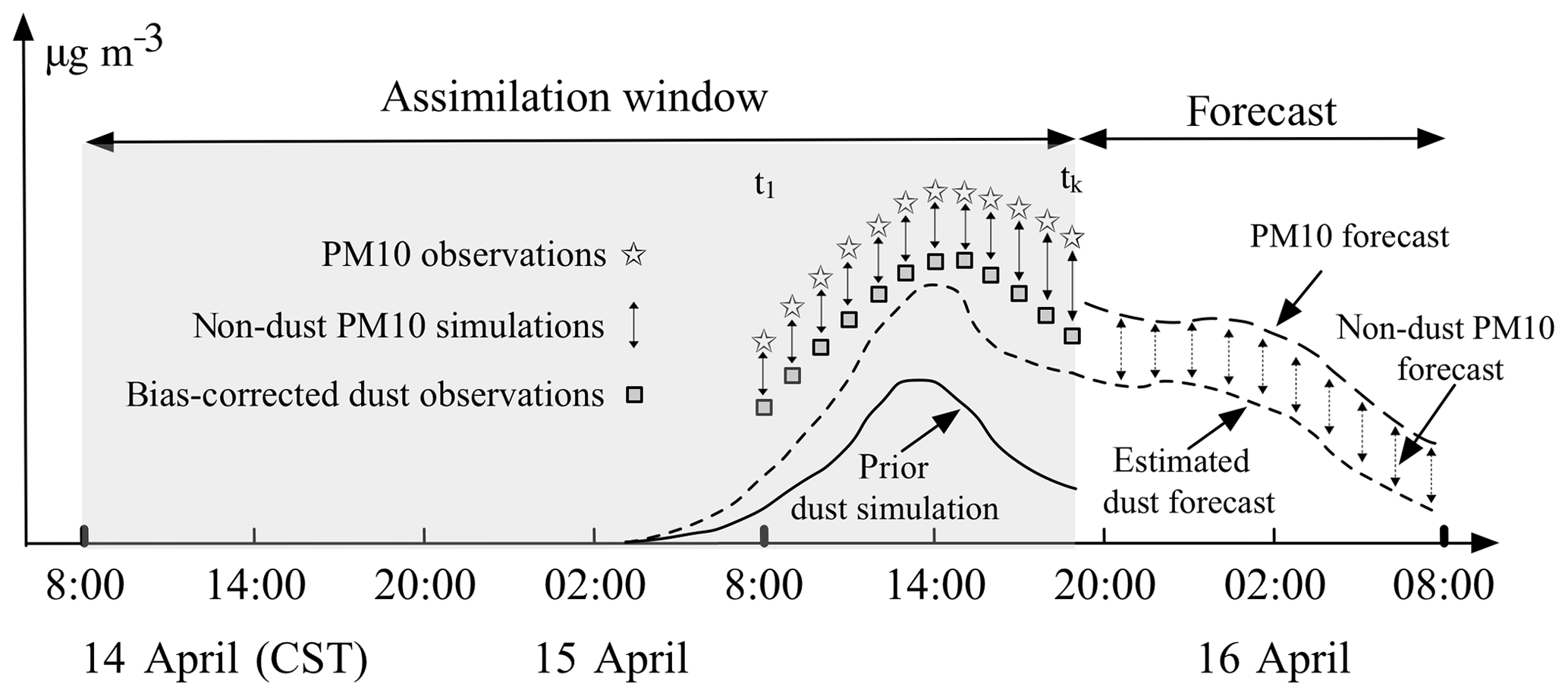
Figure 2 shows a timeline for the assimilation experiment around the April 2015 dust event, which is very similar to what was used in Jin et al. (2018). The dust event has a short duration, and therefore only a single assimilation window with a length of 36 h is used. The dust emissions take place at the start of the window, while the observations become available at the end of the window since they are located downwind from the source region (see Fig. 1). A long assimilation window is therefore necessary in order to estimate the correct emission parameters given the observations.

When we perform the assimilation analysis on 15 April, 19:00 China standard time (for all times throughout the paper), only the dust observations from 15 April, 08:00 to 19:00, will be assimilated and they are calculated by subtracting the non-dust part (CTM based or ML based) from the PM₁₀ observations. After the analysis, the simulation model is used to perform a dust forecast for the next 12 h using the newly estimated emission parameters. A fully aerosol PM₁₀ forecast will then be calculated by adding the dust forecast and non-dust aerosol forecast, where the latter again originates from either the CTM or the machine-learning model.

3 Observation bias correction methods

Two systems are introduced to correct the non-dust bias when using PM₁₀ observations in a dust assimilation. The first one is the CTM LOTOS-EUROS/non-dust that simulates the physical processes of the non-dust aerosols. The second is the machine-learning model that estimates the non-dust aerosol based on historical records. The following sections describe the two methods in more detail.

3.1 Chemistry transport model (LOTOS-EUROS/non-dust)

The regional CTM LOTOS-EUROS/non-dust is configured similar to LOTOS-EUROS/dust used in the assimilation, but now includes all trace gases and non-dust aerosols. The configuration is similar to what is used for daily air quality simulations over China as described in Timmermans et al. (2017). Anthropogenic emissions are taken from the Multi-resolution Emission Inventory for China (MEIC) (http://www.meicmodel.org, last access: 1 July 2019). Natural emissions included are the sea salts that are calculated online, biogenic emissions that are calculated online using MEGAN (Guenther et al., 2006), and wildfires which were taken from the operational GRAS product (Kaiser et al., 2012). The LOTOS-EUROS full aerosol operational forecast over this modeling domain is released via the MarcoPolo–Panda projects (http://www.marcopolo-panda.eu/, last access: 1 July 2019).

The operational CTM LOTOS-EUROS over China is in its early phase of development as well as the other six CTMs used in the MarcoPolo–Panda projects. The purpose of these projects is to diagnose statistical differences between the ensemble model simulations and observations. An important objective is to determine ways by which the models can be improved. These differences are mostly attributed to inaccuracy in the weather forecast and errors in the adopted surface emissions (Brasseur et al., 2019; Petersen et al., 2019). Indeed, there is room for minimizing the forecast–observation differences using nudging methods like data assimilation, which requires considerable efforts and is not yet exploited in that study.

3.2 Machine learning for non-dust PM₁₀ simulation

Given a set of training data, a machine-learning algorithm attempts to find the relation between input and output. When a proper model is used, the machine-learning algorithm can learn to reproduce the complex behaviors of a dynamic system. The description is purely based on the data; physical knowledge is not included. Machine-learning algorithms are popular tools to forecast air quality indices using historical records (Li et al., 2016; Fan et al., 2017; Chen et al., 2018; Lin et al., 2019). In this study, the machine-learning algorithm used is the long short-term memory (LSTM) neural network, which has demonstrated its ability in predicting time series problems (Li et al., 2017b).

The LSTM operator ℒ, which is configured with parameters θ, for predicting non-dust PM₁₀ can be described as

$$\begin{array}{}\text{(7)}& {\mathit{b}}^{t_{\mathrm{0}}+t}={\mathcal{L}}_{\mathit{\theta }}({\mathit{x}}^{t_{\mathrm{0}}},{\mathit{x}}^{t_{\mathrm{0}}-\mathrm{1}},\mathrm{\dots },{\mathit{x}}^{t_{\mathrm{0}}-m+\mathrm{1}}),\end{array}$$

where ${\mathit{b}}^{t_{\mathrm{0}}+t}$ represents the predictor, which is in this study the non-dust PM₁₀ concentration forecast t hours in advance. The temporal correlation between the input and output features declines when t increases. In our system, the maximum forecast period t is 12 h. The input vectors ${\mathit{x}}^{t_{\mathrm{0}}},{\mathit{x}}^{t_{\mathrm{0}}-\mathrm{1}},\mathrm{\dots },{\mathit{x}}^{t_{\mathrm{0}}-m+\mathrm{1}}$ are the observed data of the past m hours, which is set as 18 h empirically. The input vectors consist of

• hourly observations of PM_2.5, SO₂, NO₂, O₃, and CO from the ground-based air quality network described in Sect. 2.2;

• observations of PM_2.5 at the nearby sites;

• local meteorological data (temperature and dew point at 2 m, wind speed at 10 m), which are taken from the LOTOS-EUROS model input and originate from the European Centre for Medium-Range Weather Forecasts (ECMWF).

The LSTM neural network parameters θ are determined by minimizing the objective function J_θ that represents the mean-squared error of predictors b with respect to the measured values y^b:

$$\begin{array}{}\text{(8)}& J_{\mathit{\theta }}={\displaystyle \frac{\mathrm{1}}{m}}\sum _{i=\mathrm{1}}^m({\mathit{b}}_i-{\mathit{y}}_i^b{)}^{\mathrm{2}}.\end{array}$$

The training dataset covers the period from January 2013 to March 2015. In other words, the LSTM model ℒ is trained to best fit the samples from this period. The two months April and May 2015 in which the studied dust event occurred are set as the testing period.

Dust storms themselves occur with very low frequency. To our knowledge, the studied dust event is the most severe one since 2002, and there are no such large-scale dust events recorded in our training period. Note that cities that are close to the Gobi and Mongolia deserts might have experienced several small-scale dust events with a limited increase in dust concentrations. However, the machine learning tries to find the global best fits for the whole training dataset. The default learning rate, which determines the weights are updated during training, on a simple sample is 10⁻⁴ in our machine-learning algorithm. Therefore, the PM₁₀ records y^b are very close to the non-dust PM₁₀ concentrations, and the rare dust event records are not excluded from the training dataset for convenience and for the expected little impact on the training result. The regression model ℒ is thus assumed to reflect only the relation between input features and the non-dust PM₁₀.

Note that including PM₁₀ observations in the series of input vectors will certainly improve the skill of the machine-learning forecasts. However, the LSTM model would then lack the ability to discriminate between the dust and non-dust fractions in PM₁₀ during a dust event. Earlier studies showed that the input variables, including PM_2.5, are independent of the dust storm as illustrated in Jin et al. (2018).

For the non-dust PM₁₀ machine-learning forecasts in a given site, observations from its nearby sites are also vital and are used in two ways. First, missing data records are unavoidable in an air quality monitoring network, while the LSTM model training requires an uninterrupted time series of features. In this study, data interpolations of air quality measurements (PM₁₀, PM_2.5, SO₂, NO₂, O₃, and CO) are performed using both a linear interpolation and a k-nearest-neighbor algorithm (Zhang, 2012) if a site has no more than 30 % of missing data. Otherwise, all the measurements at the given sites are abandoned. Generally, more information available from the nearby sites will result in a more accurate interpolation. Second, learning in the presence of data errors is pervasive in machine learning, and the measurements from nearby stations are used to limit their influence. Data errors occur due to incorrect sensor readings, software bugs in the data processing pipeline, or even inaccurate data interpolation. Statistical analysis tests have been conducted which did not only indicate a strong correlation between the non-dust PM₁₀ and air quality measurements at the given sites, but also show that the predictor (non-dust PM₁₀) is correlated with the observation indices (especially the PM_2.5) at its nearby sites. In order to eliminate errors caused by incorrect inputs at the modeling site, the measurements at the nearby stations are considered to be the essential indices. In this study, a data instance will only be selected for training the LSTM model if there is at least one nearby site within an empirical radius 0.8^∘ (approx. 80 km), and a maximum of three nearby sites will be randomly selected where observation stations are densely distributed. To save the computation costs on machine-learning model training, only PM_2.5 from nearby sites is included as input in this study.

The machine-learning model for non-dust PM₁₀ forecast is trained site by site, with the hyper-parameters shown in Table 1. With the following hyper-parameters, the machine-learning model training takes several minutes for each site. The training at each site is independent; hence, the whole workload is highly parallelizable.

Table 1 LSTM hyper-parameters.

Figure 1 presents the original field observation network (N≈1500) established by the China Ministry of Environmental Protection (MEP) up to 2018, as well as the sites (N=1351) where LSTM-based non-dust forecasts are performed. It is clear that the LSTM forecast cannot be performed at each monitoring site. A few of the sites are skipped due to the lack of nearby sites; the rest are skipped because of a high data missing rate in the training period.

3.3 Evaluation of non-dust PM₁₀ bias corrections

Our two bias models, LOTOS-EUROS/non-dust and LSTM, could both be used for air quality forecast operationally when there is no dust storm. Once a dust storm is observed, the dust emission inversion system will be enabled, and the two non-dust PM₁₀ models will then be used in dust observation bias correction. The forecasts are expected to have a good performance when dust is not present and to underestimate the PM₁₀ levels in the case of dust storms.

Both CTM LOTOS-EUROS and LSTM are tested to forecast non-dust PM₁₀ over April–May 2015. This period includes the 2–3-day dust event that is used as a test case for the assimilation. Figure 3a–c show density plots comparing PM₁₀ observations with either LOTOS-EUROS/non-dust forecasts or LSTM forecast 0 and 12 h in advance.

The CTM LOTOS-EUROS/non-dust in general underestimates the non-dust PM₁₀. The forecast results in a relatively large root-mean-square error (RMSE) of 89.4 µg m⁻³. This could be explained by the fact that not all types of particulate matters, such as secondary organic aerosols, are included in the model, and some aerosol emissions are very difficult to estimate (e.g., wood burning by households). The two LSTM forecasts show on average a good agreement with the observations. The RMSEs of the forecasts by the two machine-learning models in the 2 years of the training period are reduced to 55.9 and 60.7 µg m⁻³, and in the 2-month test period (excluding the dust event from 14 to 16 April) they also stay at comparable low levels of 58.6 and 60.2 µg m⁻³. As expected, a smaller forecast period t=0 h gives a better result than the forecast over 12 h.

The scatters in the dust period (14–16 April) are denoted using different markers in Fig. 3. The underestimation of PM₁₀ during the dust period (14–16 April) is visible in the bottom right corners of these plots.

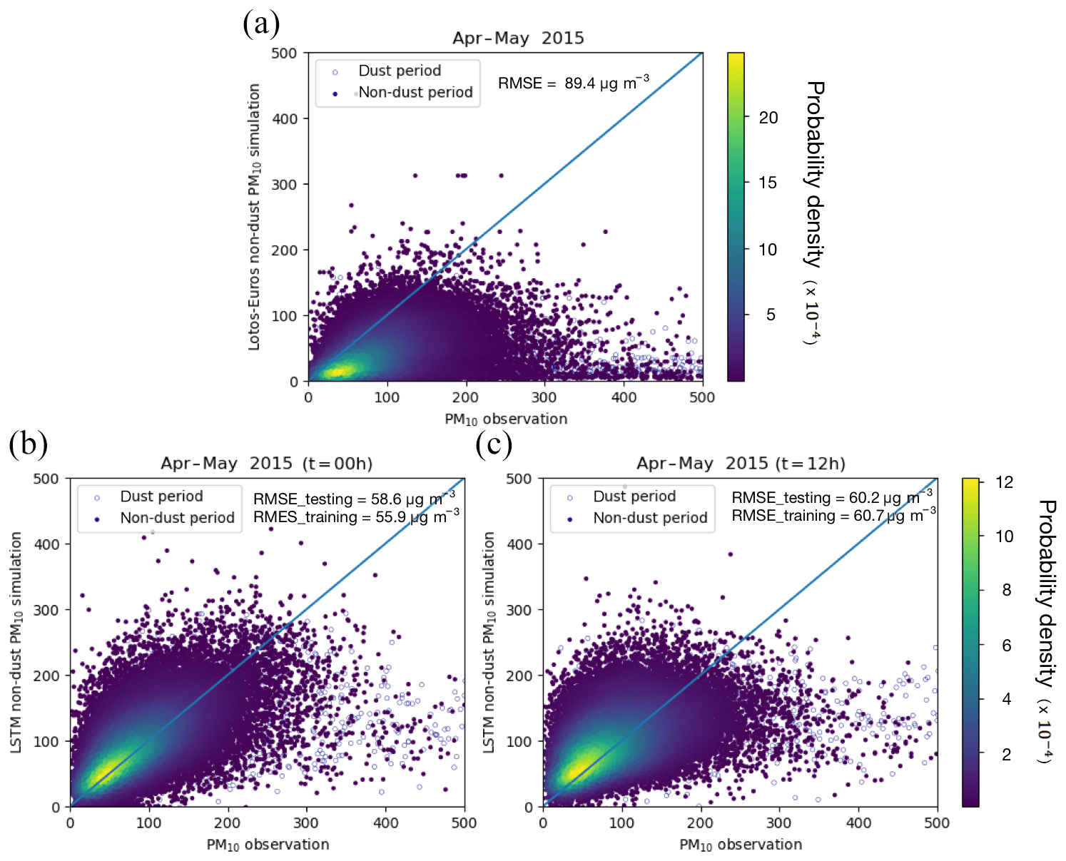
Figure 3 Non-dust PM₁₀ simulation evaluations. (a) LOTOS-EUROS/non-dust forecast vs. PM₁₀ measurements; (b) LSTM forecast 0 h in advance vs. PM₁₀ measurements; (c) LSTM forecast 12 h in advance vs. PM₁₀ measurements (note that the solid circles show the 5 % random samples over the non-dust period from April to May 2015 while the hollow ones denote the 5 % random ones from the dust period (14–16 April)).

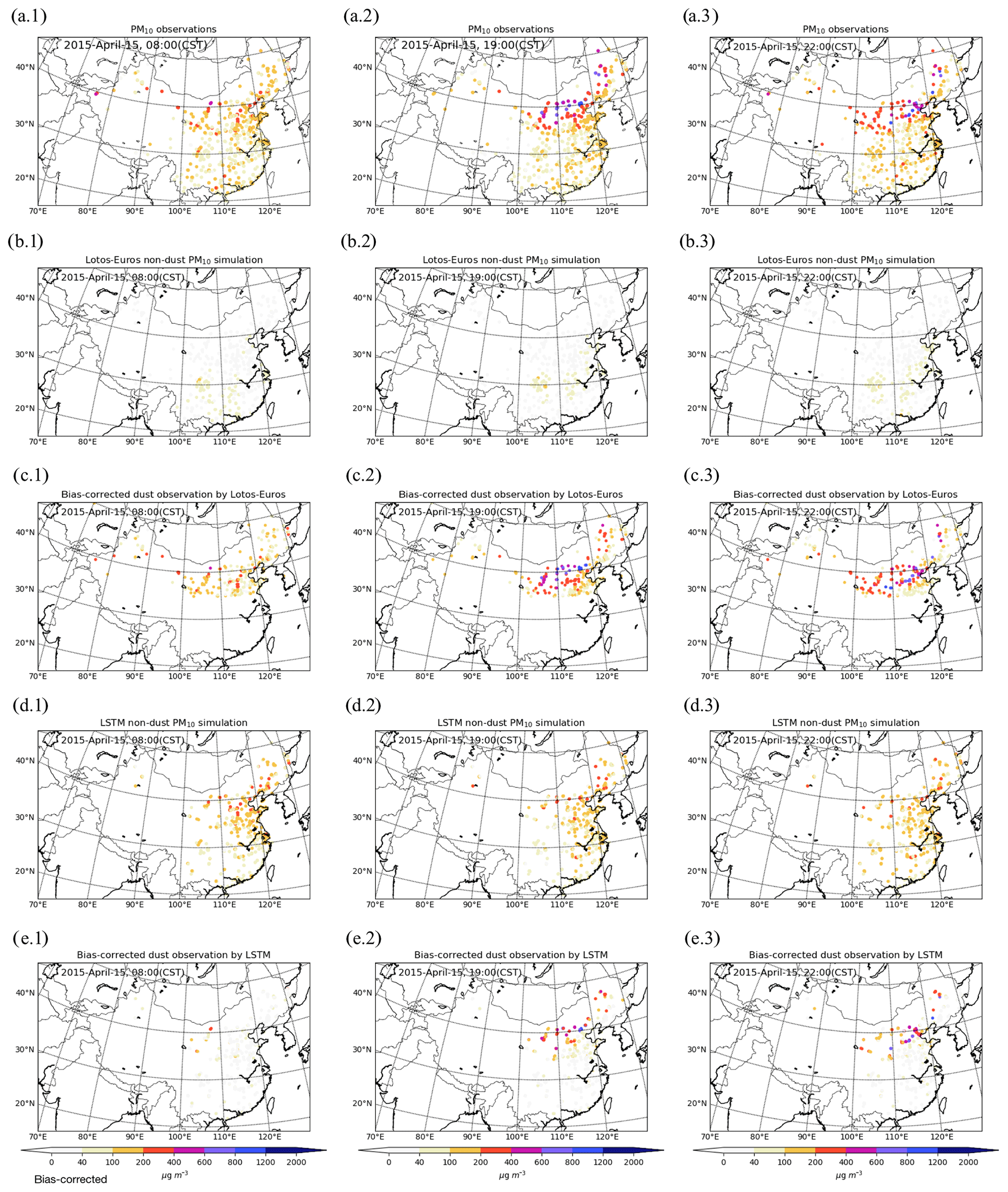
Figure 4 Original PM₁₀ measurements (a.1–a.3), LOTOS-EUROS/non-dust simulated PM₁₀ (b.1–b.3), the corresponding bias-corrected dust observations (c.1–c.3), LSTM-predicted non-dust PM₁₀ (d.1–d.3), and the derived dust observations (e.1–e.3) at three time snapshots: 15 April, 08:00 (a.1–e.1), 19:00 (a.2–e.2), and 22:00 (a.3–e.3).

When we perform the assimilation analysis on 15 April, 19:00, the short period of t=0 h forecast will be treated as the non-dust levels in the bias correction of the original PM₁₀ measurements. Note that here t=0 forecasts denote the forecasts are valid at each specific snapshot of the observations, while the 12 h forecasts are valid 12 h in advance; e.g., the non-dust PM₁₀ forecast (12 h) on 16 April at 07:00 is valid on 15 April at 19:00. Subsequently, the bias-corrected data are used to estimate the dust emissions over the past 36 h window. Obviously, one important aim of the assimilation is to make a better forecast, in this study, the forecast skills will be evaluated in the following 12 h from 15 April, 19:00. In addition, the forecast is assessed by comparing the combined PM₁₀ forecasts to PM₁₀ observations. The LSTM forecast with t=12 h in advance will be added to the dust storm forecast to build the combined aerosol forecast.

Figure 5 Time series of PM₁₀ measurements and LOTOS-EUROS/non-dust- and LSTM-predicted PM₁₀ levels at six cities: Hohhot, Changchun, Beijing, Baoding, Xingtai, and Yulin. LE: LOTOS-EUROS; LSTM: long short-term memory.

3.3.1 Spatial patterns at observation sites

To assess our two non-dust PM₁₀ models, Fig. 4 shows the snapshots of the PM₁₀ measurements, LOTOS-EUROS/non-dust simulations, LSTM forecasts, and the corresponding bias-corrected dust observations at three time stamps: 15 April 08:00, 19:00, and 22:00. These first two moments are the start and end of the observation interval in the assimilation window (only observations from the last 12 h of the assimilation window are assimilated as shown in Fig. 2), and observations at 22:00 are treated as independent data for cross-validation. At 08:00, only few stations close to the dust source area have already observed the dust storm. Some of the sites in central China observed high PM₁₀ concentrations, which are believed to be caused by the presence of non-dust aerosols. Nearly all the stations in north China reported this dust storm at 19:00 and 22:00, as a band covering central and northeast China; see Fig. 4a.2–a.3. Figure 4b.1–b.3 show that the LOTOS-EUROS/non-dust model forecasts quite stable and constant non-dust PM₁₀ levels; most of the simulated values are less than 100 µg m⁻³. Subsequently, the corresponding bias-corrected dust measurements (see Fig. 4c.1–c.3) are very similar to the original PM₁₀ observations. This could be problematic when trying to measure the dust storm from the PM₁₀ observations; for instance at 08:00 in Fig. 4c.1, according to the bias-corrected observations the dust storm seems to have already reached central China, which was probably not the case. In comparison, the LSTM-based bias-corrected dust observations (see Fig. 4e.1–e.3), which are calculated by subtracting the LSTM non-dust part (see Fig. 4d.1–d.3) from the raw PM₁₀ measurements, are close to our expectations. Only for sites that are very close to the source regions' high dust concentrations are derived at 08:00, while for the other sites hardly any dust is derived. At 19:00, 11 h later, at half of the stations in the north of the domain high dust concentrations are derived. In the southeast of the domain, the derived dust concentrations remain almost zero since the dust plume did not arrive there yet. At 22:00, the plume is moved further south, and the dust load closer to the source region started to decrease.

3.3.2 Time series

To further evaluate the two bias correction methods, Fig. 5 shows the time series at the following selected cities: Hohhot, Changchun, Beijing, Baoding, Xingtai, and Yulin. The location of these cities/sites can be found in Fig. 1. These cities were selected because they all experienced severe pollution and illustrated the general performance of the LOTOS-EUROS/non-dust and LSTM methods. In addition, each of these cities has at least four monitoring sites, which assured a high accuracy.

The LOTOS-EUROS grid cells with the selected sites all include other observation sites as well, and to illustrate the spread in the observations the maximum and minimum observed values in the grid cell are added to the time series too. Similarly, the LSTM non-dust PM₁₀ simulation is given together with the spread within the grid cell.

Before the dust storm arrives at these cites, the LSTM model reproduces the variations in PM₁₀ rather well. Some errors are present, for example as can be seen on 14 April from 12:00 to 23:00 in Yulin. After the arrival of the dust storm, the PM₁₀ observations strongly increase, while the LSTM non-dust fraction remains at a low level since it is independent of the dust storm. The real dust measurement is then calculated by subtracting the non-dust part from the raw PM₁₀ observations.

The LOTOS-EUROS/non-dust simulations underestimate the non-dust PM₁₀ at all six locations. Thus, the derived bias-corrected dust observations overestimate the actual dust load, and this will affect the dust assimilation results.

4 Data assimilation experiments

Three different sets of observations are now available for assimilation in the dust model: the original PM₁₀ observations, the PM₁₀ observations with LOTOS-EUROS bias correction, and the PM₁₀ observations with machine-learning bias correction. The results have been compared in terms of the a posteriori dust emission fields and surface dust concentrations.

A practical use of assimilated concentrations is to use them as a start point for a forecast. This could be used to provide early information about the arrival of the dust plume and the expected dust level. The dust forecast after the end of the assimilation window at 15 April 19:00 uses the newly estimated emissions. Apart from the dust concentrations, the forecast will also be evaluated in terms of skill scores for the total PM₁₀ concentrations in Sect. 4.3.

4.1 Observation error configuration

A key element of the data assimilation system is the observation error covariance matrix R. This covariance quantifies the possible difference between simulations and observations. The observations with a smaller error have a higher weight in the assimilation process.

In related works, the dust observation errors were usually empirically quantified. Lin et al. (2008) assumed that the observation error is proportional to the measurement with a constant factor of 10 %. Jin et al. (2018) used a similar error setting but also assigned a larger error to low-value measurements since the model might easily result in relatively large errors when simulating minor dust loads.

Theoretically, the observation uncertainties are due to the representation errors as well as the measurement errors, while the former is widely considered the largest source. Limited by the computation resources, our dust model uses a spatial resolution of 25 km, while the in situ measurements cover much less of the atmosphere surrounding them (Schutgens et al., 2016). This of course limits our capability of resolving the fine-scale fields that are reflected in observation spaces. Therefore, the spatial representation error is assumed to be the dominant error source and taken into the account in approximating the observation uncertainties. In addition, the error due to the different bias correction terms is indeed another source. It is not yet considered in this study but will be exploited for a more accurate assimilation operation in our future work.

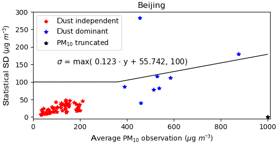
Figure 6 Average vs. standard deviation of the hourly PM₁₀ observations ranges from 14 April at 08:00 to 17 April at 07:00 in the grid cell of Beijing. See Fig. 5c for the time series.

The spatial representation error quantification itself is a complex task. It could be calculated through comparing the model simulations at different scales of resolutions. In this study, the availability of multiple measurement sites in a single model grid cell provides an alternative way to quantify the representation error. When multiple observations are present, the statistical error in the observed values reflects the spatial representation uncertainty. An example is the grid cell covering the city of Beijing, where observations from 12 different field stations are available. Note that it is the grid cell which has the most monitoring stations. The spread of the hourly measurements is shown in Fig. 5c. For each hour, the standard deviation of the measured PM₁₀ values is plotted against the mean in Fig. 6, where the red markers represent “regular” polluted conditions, and the blue markers the dust event. The result shows that the spread in the observations closely agrees with the average pollution level during the dust event. Based on this result, a simple linear regression is used to obtain a parametrization for the observation representation error:

$$\begin{array}{}\text{(9)}& \mathit{\sigma }=max(a\cdot y+b,{\mathit{\sigma }}_{\text{min}})\left[\mathrm{\mu }\mathrm{g}{\mathrm{m}}^{-\mathrm{3}}\right],\end{array}$$

where a=0.12 and b=55.7 are the linear regression parameters based on the dust event data (blue markers). It should be noted that the observation sites in Beijing truncate observations at a maximum of 1000 µg m⁻³, and therefore observations close to this number are not used since the true values might have been much higher. A minimum observation representation uncertainty of σ_min=100 µg m⁻³ is used for the dust observations (PM₁₀ with bias correction) to avoid a too strong impact of low-value observations (hardly dust) on the estimation of dust emissions. In case the simulation model estimates dust concentrations at the surface while in reality the plume is elevated, the low-value observations might lead to an unrealistically strong decrease in the dust emissions.

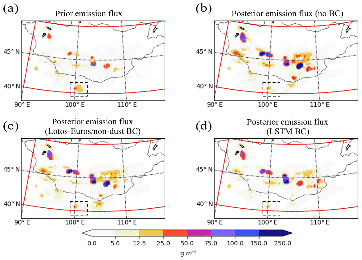
Figure 7 Accumulated dust emission map ℱ between 14 April at 08:00 and 15 April at 19:00 of the a priori model (a) or (b) a posteriori estimates using the original PM₁₀ observations, (c) LOTOS-EUROS, or (d) LSTM-based bias-corrected dust measurements. BC: bias correction.

The representation uncertainty has already been validated to fluctuate in space (Schutgens et al., 2016). However, for most other grid cells the number of observation sites is simply one, which makes it difficult to parametrize a representation error in a similar way. Therefore, the representation error parametrized for Beijing is used for all other locations too.

Note that the raw PM₁₀ and the bias-corrected dust measurements might have different uncertainties in representing the real dust storm level. This is not yet taken into account in our study, and the three types of the assimilated measurements, raw PM₁₀ and bias-corrected dust observation using either a CTM or machine learning, are all configured with the same observation error in Eq. (9). In addition, all the measurements are assumed to be independent; hence, the observation error covariance R is diagonal.

4.2 Dust emission estimation

To evaluate the a posteriori dust emission field that is obtained by assimilation of the bias-corrected dust observations, an emission index ℱ_i (g m⁻²) is defined as in Jin et al. (2018). The index represents the accumulated dust emission in a cell i between 14 April 08:00 and 15 April 19:00. Figure 7 shows the emission index map of the a priori model and a posteriori emissions obtained from assimilation of either the original PM₁₀ observations, or the LOTOS-EUROS- or LSTM-based bias-corrected dust measurements.

As shown in Fig. 7a, the a priori emission was in general rather weak, which resulted in an underestimated surface dust concentration simulation as can be seen for example in Fig. 8a.1–a.2. The a posteriori emissions are almost everywhere higher than the a priori. An exception is the region marked in black, where the a priori emissions are higher. The emissions from this black-dashed region contributed to a too-early arrival of the dust peak in the model cells over Hohhot and Xingtai as shown in Fig. 9a and c.

Figure 7b shows the emission index ℱ that results from directly assimilating the original PM₁₀ measurements. As expected the estimated emissions are higher than those obtained by assimilating the bias-corrected observations since all airborne aerosols observed are considered to be dust. In comparison, the assimilation with the LSTM baseline removed data results at a modest emission level as shown in Fig. 7d. The emissions estimated with LOTOS-EUROS-based bias-corrected observations are in between since the resulting dust observations also overestimate the actual dust loads compared to the LSTM-based bias-corrected dust measurements.

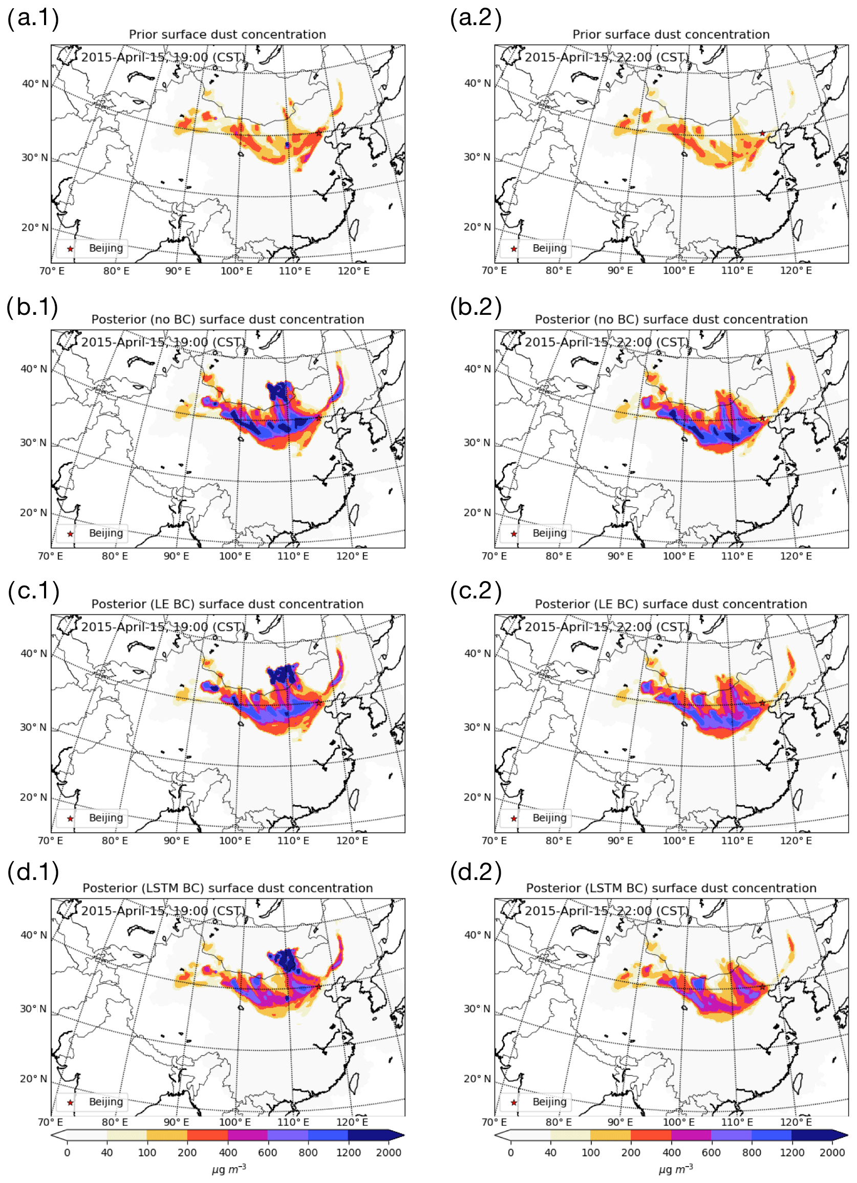
Figure 8 Surface dust concentration of a priori (a.1–a.2), a posteriori using no bias-corrected (no BC) data (b.1– b.2), a posteriori using LOTOS-EUROS/non-dust bias-corrected (LE BC) data (c.1–c.2), and a posteriori using no bias-corrected (LSTM BC) data (d.1–d.2) on 15 April at 19:00 (a.1–d.1) and 22:00 (a.2–d.2).

4.3 Dust simulation and forecast skill

Figure 8a–d show the dust simulations at the surface layer at the end of the assimilation window (15 April, 19:00, left column) and the forecast 3 h later (22:00, right column) using the newly estimated emission field. Note that the average dust concentration over the affected downwind regions reached a peak around 22:00. Compared to background simulations in Jin et al. (2018), the a priori model simulations have been improved by disabling the topography-based preference factor as mentioned in Sect. 2.1; however, a large difference from the bias-corrected PM₁₀ observations in Fig. 4e is still present.

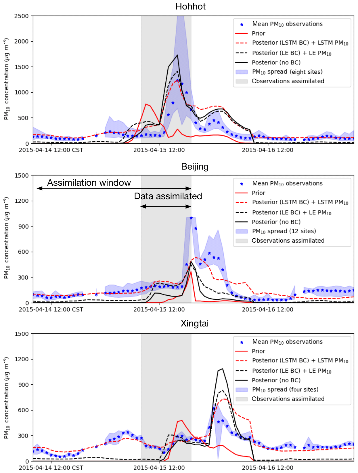
Figure 9 Time series of a posteriori dust concentration and PM₁₀ observations in three cities: Hohhot, Beijing, Xingtai (observations in the gray shaded part are assimilated).

The a posteriori concentrations in Fig. 8b.1–b.2 are the result of assimilating the original PM₁₀ observations shown in Fig. 4a.1–a.2. As expected, these lead to the highest simulated dust concentrations since all the aerosols observed are assumed to represent dust. Especially in the center of the plume, the dust concentration can be as large as 2000 µg m⁻³. Figure 8c.1–c.2 show the results when using the LOTOS-EUROS/non-dust bias-corrected PM₁₀ observations as dust, and although concentrations are lower, they are still likely to overestimate the real dust levels. The a posteriori results using the LSTM bias-corrected measurements provide the lowest dust concentrations as shown in Fig. 8d. Only in the grid cells that are close to the source region, do the surface dust concentration reach values as large as 2000 µg m⁻³, while in the downwind areas the maximum dust concentrations are usually below 1200 µg m⁻³.

To illustrate the improvements of assimilating bias-corrected measurements, Fig. 9 shows the observed and simulated PM₁₀ concentrations in the aforementioned grid cells covering Hohhot, Beijing, and Xingtai. These locations are neither the best nor the worst examples, but illustrate typical results and challenges to be solved in future. For a fair comparison with the PM₁₀ observations, the non-dust aerosol concentrations obtained from either LOTOS-EUROS/non-dust or LSTM were added to the dust simulations from the inversion system.

Figure 10 Time series of root-mean-square error compared to the ground PM₁₀. The assimilation window is set from 14 April at 08:00 to 15 April at 19:00, and PM₁₀ observations in the gray shaded area are assimilated.

The site Hohhot is close to the main dust source region. The a priori model simulated the arrival of the dust plume 8 h before it was actually visible in the PM₁₀ observations. The assimilation of the observations is able to produce simulations in which the dust plume arrives at the correct time. The assimilation with LSTM bias-corrected data has the best performance, with the peak of the simulated concentrations (dust plus bias) most close to the observed PM₁₀. During the forecast period (t> 15 April, 19:00), all three assimilation-based forecasts show a decline in concentrations, which slightly overestimate the observations. This can be explained from the fact that the dust storm is a strong flow-dependent phenomenon in which concentrations at a certain location are strongly correlated to earlier concentrations at upwind locations. For Hohhot, only a limited number of observation sites are located upwind, and therefore hardly any data are available to constrain the concentrations at this location. To improve the forecast at Hohhot it will be necessary to have additional observation data, for example from sites actually within the source region, or from satellites observing the aerosol load over the source region (Jin et al., 2019).

For the grid cell Beijing, which is located further downwind from the dust source region, the arrival of the dust peak is correctly simulated. However, the amplitude of the concentration peak is underestimated compared to the average PM₁₀ observations. As can be seen in Fig. 8, the dust plume forms a rather small band over central and northeast China. In each of the three assimilations, the dust concentrations in the band are rather low around Beijing. This suggests that the simulation model simply is not able to increase the dust concentrations here, for example because of uncertainties in the meteorological data, a removal of dust that is too efficient, or because some local sources of dust are absent (equally, non-dust PM₁₀ levels are underestimated).

The grid cell Xingtai is located more to the south, and the model is able to simulate high dust concentrations here. The a priori model simulates the arrival of a first dust peak already at 13:00, which is however not visible in the PM₁₀ data. The assimilation postpones the arrival of the main dust, which according to the measurements takes place around 22:00 and is already in the forecast period. The forecast simulations all overestimate the amplitude of the peak, especially when using the original PM₁₀ data as proxy for dust. The assimilation with the LSTM-based baseline removal shows the best agreement with the observations.

4.4 Evaluation of forecast skill

To evaluate the forecast skill of the assimilation(s), the root-mean-square error (RMSE) of the reference and three a posteriori fully aerosol simulations (dust forecasts plus non-dust predictions) with respect to the observed PM₁₀ over the whole observation sites has been computed for each hour. A time series of this RMSE is shown in Fig. 10; after the assimilation window (marked period), the results are based on the forecast simulations. The a priori RMSE values at the end of the assimilation window and during the forecast are about 200–250 µg m⁻³. Direct assimilation of the original PM₁₀ measurement actually increases these values to above 300 µg m⁻³ during the forecast since dust concentrations become strongly overestimated. Assimilation of the LOTOS-EUROS/non-dust baseline-removed observations nonetheless reduces the RMSE, in particular within the assimilation window. The strongest decrease in RMSE is obtained using the LSTM-based baseline removal, with values of 120–200 µg m⁻³ during the forecast.

5 Summary and conclusion

In this study, a dust storm data assimilation experiment has been performed for an event over East Asia in the spring of 2015. PM₁₀ observation data from the China Ministry of Environmental Protection observing network were assimilated into a dust simulation model to estimate the dust emissions. The PM₁₀ measurements themselves are considered unbiased. They clearly show the arrival of a dust plume throughout the region due to the high spatiotemporal resolution. However, the data cannot be compared directly to dust simulations since they actually represent a sum of the dust particles and other non-dust aerosols. Direct assimilation of these measurements would introduce a bias in the assimilation system since it cannot distinguish between model and observation errors.

Two methods have been implemented to remove the non-dust part of the PM₁₀ observations during the dust event in order to use them as a dust proxy in a dust assimilation system. The first method uses a conventional regional chemistry transport model, LOTOS-EUROS/non-dust, which simulates the emission, transport, chemistry, and deposition of aerosols mainly related to anthropogenic activities. The second method uses a machine-learning model that statistically describes the relations between regular PM₁₀ concentrations (outside dust events) and available air quality and meteorological data.

The two methods to estimate the non-dust part of the PM₁₀ load have been validated. The simulations by the LOTOS-EUROS/non-dust model in general underestimate the PM₁₀ concentrations. The root-mean-square error stays at a relatively high level of 89.4 µg m⁻³. It is mainly caused by missing emissions and aerosol components such as secondary organic matter. In comparison, the data-driven machine-learning model agrees more closely with the real measurements; the RMSE declines to 58.6 µg m⁻³.

A variational data assimilation system has been used to estimate the dust emissions that led to a severe dust storm in April 2015. The system assimilated either the original PM₁₀ observations or the bias-corrected dust observations based on either LOTOS-EUROS/non-dust or the LSTM model. The a posteriori simulations using the original observations resulted in a strong overestimation of the dust concentrations since all PM₁₀ is simply attributed to dust. Using the LOTOS-EUROS/non-dust bias-corrected observations, a clear improvement on the dust simulation has been obtained, but overestimation of dust concentrations is still present. The best results are obtained when using a LSTM model to remove the non-dust part of the PM₁₀ observations, with a posteriori concentrations in good agreement with the measurements.

The dust emissions estimated using the assimilation can be used to drive a dust forecast. When the original PM₁₀ observations were used in the assimilation, the forecast skill of the system actually decreased due to the strong overestimation of dust concentrations, and the RMSE rose from on average 230 (prior forecast) to 300 µg m⁻³. Better forecasts are obtained when using the model-based and especially the machine-learning-based bias-corrected observations. The RMSE of the former was reduced to 200 µg m⁻³ while the RMSE of the latter further declined to 150 µg m⁻³.

Future work

Both our CTM and machine-learning-based bias correction methods have room for improvements. It might be useful to improve the CTM simulations by assimilating PM₁₀ observations during the hours where no dust storms are present and use these improved simulations to remove the non-dust part of the observations during an event. These additional assimilations would then involve repeated forward ensemble bias–model runs which could be computationally expensive. The machine-learning model in our non-dust PM₁₀ simulation can also be further optimized, such as using a different configuration or deeper neural network, including extra input features like non-dust PM₁₀ simulation from CTMs (Lin et al., 2019) and other related records.

We will exploit the variabilities of the representation errors comparing the model simulations at different spatial resolutions. The error from the bias correction term will also be taken into account while calculating the observation error.