the Creative Commons Attribution 4.0 License.
the Creative Commons Attribution 4.0 License.
 | 12 Jul 2018
A very limited role of tropospheric chlorine as a sink of the greenhouse gas methane
Carl A. M. Brenninkmeijer
Patrick Jöckel
Unexpectedly large seasonal phase differences between CH4 concentration and its 13C ∕ 12C isotopic ratio and their inter-annual variations observed in southern hemispheric time series have been attributed to the Cl + CH4 reaction, in which 13CH4 is discriminated strongly compared to OH + CH4, and have provided the only (indirect) evidence of a hemispheric-scale presence of oxidative cycle-relevant quantities of tropospheric atomic Cl. Our analysis of concurrent New Zealand and Antarctic time series of CH4 and CO mixing and isotope ratios shows that a corresponding 13C ∕ 12C variability is absent in CO. Using the AC-GCM EMAC model and isotopic mass balancing for comparing the periods of presumably high and low Cl, it is shown that variations in extra-tropical Southern Hemisphere Cl cannot have exceeded 0.9 × 10³ atoms cm−3. It is demonstrated that the 13C ∕ 12C ratio of CO is a sensitive indicator for the isotopic composition of reacted CH4 and therefore for its sources. Despite ambiguities about the yield of CO from CH4 oxidation (with this yield being an important factor in the budget of CO) and uncertainties about the isotopic composition of sources of CO (in particular biomass burning), the contribution of Cl to the removal of CH4 in the troposphere is probably much lower than currently assumed.
- Article
(634 KB) - Full-text XML
-
Supplement
(1063 KB) - BibTeX
- EndNote


Compared to the troposphere's main oxidant OH (hydroxyl radical), the role of Cl (atomic chlorine) for CH4 is small. A recently published detailed model-based estimate attributes ∼ 2.6 % of methane's photochemical tropospheric loss to Cl (Hossaini et al., 2016). Because this loss constitutes only a small term in the methane budget, it might be deemed irrelevant. Nevertheless, growing spatial and temporal coverage in CH4 observational data allows for top-down estimates of changes in the source–sink budget to the order of ∼ 1 %. Moreover, considering that the photochemical sink is the dominant and best-known term in the global methane budget, it makes sense to improve our calculations. The grateful aspect of this endeavour clearly is that one does not need an accurate estimate of Cl as a global tropospheric sink of CH4 as such. It would already be helpful to have independent estimates of the upper limit for this interesting sink of CH4, whose rise in the Anthropocene thus far has contributed one-fifth to global warming.
Irrespective of the implications for the CH4 budget, it stands to reason to fully understand tropospheric Cl and its chemistry in different air masses, from marine boundary layer air to strongly polluted air masses, and several studies address these complex processes. It is also clear that the budget of a species as fickle as atomic chlorine is hard to determine in general terms (which forms a less grateful aspect of “assessing chlorine”). Nevertheless, a new effort – in assessing chlorine's role on a larger than regional scale, on the basis of trace gas measurements, may be useful.
Even more so than for OH, estimates of the abundance of Cl atoms are chiefly based on indirect evidence. Direct measurements of OH concentrations ([OH]) are difficult and rare, and for [Cl] this is even much more so. Therefore, the method (by choice or opportunity) is indirect. Not only are indirect measurements easier, the use of trace gases that react with OH and Cl also has the advantage that space- and time-averaged estimates are obtainable. In this case, one can select for instance two hydrocarbons, one of which has a comparatively high reactivity to Cl. The change in ratio between the two hydrocarbon concentrations gives information on [Cl] relative to [OH].
Using stable isotope ratio information offers another such indirect method. The intrinsic advantage here is that one can use a single trace gas, a single hydrocarbon, or even the much studied greenhouse gas CH4 itself. Although the rate coefficient for the reaction of OH with 12CH4 is only ∼ 4 ‰ faster than that with 13CH4 (Saueressig et al., 2001), for Cl + CH4 the difference is much larger (Saueressig et al., 1995; Crowley et al., 1999), viz. 63–75 ‰ (at the range of tropospheric temperatures). Broadly speaking, the presence of 13C-enriched CH4 points to reaction with Cl. If this were not enough, one could measure the D ∕ H ratio of CH4 and obtain additional valuable information because of the large isotope fractionation (KIE, kinetic isotope effect, formerly and still expressed using the kinetic fractionation constant ε= α−1) and the differences between the KIEs for 13C and D. A recent paper (Whitehill et al., 2017) reports changes in the clumped isotopic composition of CH4 in reaction with Cl based on laboratory experiments, raising hope that clumped isotope measurements (which are very difficult) may in an additional way assist to further assess the role of Cl in the oxidation of CH4 in the atmosphere.
An advantage is that the “stable isotope method” in principle removes the uncertainty about the variability induced by having to use two different trace gas species, each of which may have an independent, variable source. Routinely overlooked is another (principle) advantage of stable isotope analysis offered in the case of atmospheric CH4 → CO conversion, namely measurement of the isotopic composition of the reaction product CO. Even though variations in [CO] may not be resolvable due to the large spatio-temporal variability of its sources and sink, its 13C ∕ 12C ratio may well tell a clearer story. This is the added advantage of the stable isotope method (we note that the lifetime of 14C is sufficiently long to render much of what is stated to also apply to this well-known radioisotope, but there are complications on which we cannot dwell here).
In this way the presence of Cl during Antarctic ozone hole conditions could be inferred in an independent fashion (Brenninkmeijer et al., 1996). Not only did the CH4 inventory become slightly enriched in 13C due to the large KIE in Cl + CH4, the CO ensuing from CH4 resulted in strong depletions in the background 13CO. There are at least three reasons for the strong isotope depletion. First, CO concentrations are low in the stratosphere and the in situ produced CO had a large impact. Second, the 13C content of CH4 is characteristically low due to its chiefly bacterial origin. Third, and this is an important point mentioned above, the 13C KIE for Cl + CH4 happens to be very large. The combination of these effects renders the stable isotope analysis of CO a sensitive indicator. Dealing with tropospheric Cl, the same principle has been applied during springtime tropospheric ozone depletion events in the Arctic. Short-term bursts of free Cl could be inferred from concomitant decreases in δ13C(CO) within a per mil1 range (Röckmann et al., 1999).
We record that there also is a removal of CO by reaction with Cl atoms, with the rate constant typically being 6 times smaller than that of CO + OH. Given this very low rate coefficient and the low Cl ∕ OH ratio, only an extremely large KIE in the CO + Cl reaction could impact significantly on δ13C of the CO inventory. In contrast, the rate constant for CH4 + Cl is typically 20 times larger than that for CH4 + OH. Cl is not expected to play a significant role in atmospheric CO removal, except possibly at polar sunrise (Hewitt et al., 1996) and in some stratospheric chemistry analyses (see, for example, Müller et al., 1996; Sander et al., 2011b). None of a few of papers on tropospheric CO thus mentions Cl as a sink for CO because of its negligible share; fortunately, because the reaction product is not so nice.
In this brief account we cannot do justice to all tropospheric Cl-related papers in the literature and we refer to the recent model-based paper by Hossaini et al. (2016) and references therein. In comparison with OH, which is recycled in about two of three reactions in the troposphere (Lelieveld et al., 2016), the role of recycling of Cl is lower and not well known. The presence of Cl in the marine boundary layer has been inferred using hydrocarbon measurements (early study by Parrish et al., 1993) and likewise during polar sunrise (Jobson et al., 1994), Cl2 has been measured in situ in coastal air (Spicer et al., 1998) and in the Arctic (Liao et al., 2014). ClNO2, which is an important precursor, has been measured (Osthoff et al., 2008 and Thornton et al., 2010), also by Young et al. (2012), although they found no Cl fingerprint in hydrocarbon ratios.
Recently, Baker et al. (2016) inferred the presence of Cl in pollution outflow from continental Asia using hydrocarbon measurements on air samples collected at cruise altitude by the CARIBIC Lufthansa Airbus aircraft observatory. Before that, Baker et al. (2011) had likewise inferred that Cl is formed in an emission plume of the Eyjafjallajökull volcano probed by the same CARIBIC A340 aircraft. All these and other publications discuss the presence of Cl in a variety of tropospheric environments wrestling with the complexity of its chemistry and paucity of experimental data.
The additional importance of revisiting the role of Cl radicals in the present atmosphere actually surfaces in the reconstruction and understanding of the budget of CH4 in the past. Changes in the tropospheric burden of CH4 that occurred in the past (last glacial maximum to present) are due to changes in CH4 sources and to a minor degree to changes in OH chemistry (Levine et al., 2011b). One would a priori expect δ13C(CH4) to provide additional information on source changes, as it did for immediate past changes (Schaefer et al., 2016), were it not the case that large changes in Cl abundance may well have affected the δ13C(CH4) record (Levine et al., 2011a). If this is indeed the case, changes in Cl abundance in the past may have not affected the CH4 budget itself significantly, but may have invalidated to a certain degree the δ13C(CH4) isotope method for determining changes in sources (biogenic vs. biomass burning).
We turn our attention to a paradox concerning today's tropospheric Cl, namely: if the presence of tropospheric Cl could be inferred from 13C isotope enrichment in CH4, why is this effect not visible as concurrent isotope depletion in CO? Or, more explicitly stated, if the δ13C(CO) isotope method for Cl detection works well for the austral polar stratosphere in spring (Brenninkmeijer et al., 1996) and for the polar sunrise in the Arctic (Röckmann et al., 1999), why not so for the troposphere, or does it? Is a clear negative signal in δ13C(CO) indeed absent, and if so, does this absence allow us to cap estimates of tropospheric Cl levels?
2.1 Chlorine in the Southern Hemisphere
Because the budgets of CH4 and CO in the Southern Hemisphere (SH) are less complicated than in the Northern Hemisphere, as is shown by their compact regular seasonal cycles at remote observatories2, and because long records of CO and CH4 including isotopic data are available, we focus on the Southern Hemisphere. In the SH evidently the emphasis is on Cl generated in the marine boundary layer (MBL).
We first revisit the information on Cl based on δ13C measurements of CH4. Initially, mixing ratio and δ13C(CH4) values for shipboard collected air samples in the Pacific pointed to a large apparent sink isotope fractionation (“apparent” KIE) of 12–15 ‰ – well in excess of the aforementioned 4 ‰ from OH + CH4 – which led to the conjecture that a fraction of CH4 is removed in the MBL by Cl atoms which discriminate strongly against 13CH4 (Lowe et al., 1999; Allan et al., 2001). Following several publications exploring this effect, Allan et al. (2007) (hereinafter referred to as A07) using global modelling and observational data from the extratropical Southern Hemisphere (ETSH), confirmed a large apparent KIE and could estimate a global marine boundary layer based Cl sink for CH4 averaging at 25 Tg(CH4) yr−1.
Given this number, a first-order estimate of the accompanying response of δ13C of CO to the production of CO from Cl + CH4 can be made. Assuming a 100 % yield of CO from OH + CH4 (and likewise Cl + CH4), the 25 Tg yr−1 CH4 sink corresponds to a Cl-based annual CO production of 44 Tg yr−1, which is ∼ 1.8 % of the total CO budget. By using a δ13C value of CO of −28 ‰ (annual tropospheric average), that of CH4 of −48 ‰ and a KIE of 70 ‰, (Cl + CH4) causes a negative shift in δ13C(CO) of about 1.6 ‰. Considering that the lifetime of CO is much shorter than that of CH4 and that Cl is concentrated in the MBL, the local and/or seasonal effect on δ13C(CO) would be even larger.
Unfortunately, a negative shift in δ13C(CO) is unwelcome in attempts to close the SH CO budget using δ13C. As Manning et al. (1997) have pointed out, budget closure is only possible when the yield of CO from CH4 + OH (denoted hereinafter as λ) is assumed to be merely about 0.7. In other words, even without incorporating the formation of CO from Cl + CH4, the CH4-derived 13C-depleted fraction of CO (which is high in the ETSH at above 40 %) appeared to be too dominant and had to be reduced by assuming lower yields of CO from CH4. Soon thereafter, Bergamaschi et al. (2000) also encountered this problem in a 3-D inverse modelling study using the isotopic composition of CO and could best reconcile data and model by reducing λ to about 0.86. They do mention that incorporating CO from Cl + CH4 would require λ values as low as 0.71. Platt et al. (2004), who discuss mechanisms for the production of Cl in the marine boundary layer, also allude to the necessity to have to reduce the assumed CO yield of OH + CH4.
One difficult feature of the δ13C(CH4)-based Cl estimate was a large inter-annual variability that could not be explained. A07 identified two periods of different Cl abundance in the ETSH, namely 1994–1996, with MBL values of 28 × 103 atoms cm−3 (high-Cl period, “HC”) and 1998–2000 with much lower values, viz. 9 × 10³ atoms cm−3 (low-Cl period, “LC”). The nearly 3-fold drop in the resulting Cl + CH4 sink rate (37 to 13 Tg(CH4) yr−1, or 6.4 to 2.2 % of the total, respectively) inferred from δ13C(CH4) for the two periods is not discernible in the simultaneous δ13C(CO) record (see Sect. 2.2).
Later, Lassey et al. (2011) investigated the apparent KIE in detail and found that it can differ markedly from both the seasonal and mass-balanced KIEs. In other words, the apparent KIE derived from the seasonal changes in [CH4] and δ13C(CH4) values appeared not to properly represent the respective effects of the two KIEs. The implication is that the inferred very large range of [Cl] may be in error, and the absence of a corresponding signal in δ13C(CO) is in that respect an experimental confirmation. Below we will go into detail.
2.2 Observations in the ETSH
We scrutinise the mixing and 13C ∕ 12C ratios of CH4 and CO in the MBL air at Baring Head, New Zealand (41.41∘ S, 174.87∘ E, 85 m a.s.l., denoted hereinafter “BHD”) and at Scott Base, Antarctica (77.80∘ S, 166.67∘ E, 184 m a.s.l., denoted “SCB”)3 provided by the National Institute of Water and Atmospheric Research (NIWA, 2010). Examined in the A07 study on CH4, these data are the result of laboratory analyses of large air samples collected on a monthly to weekly basis. The collection strategy (using wind direction, CO2 mixing ratio temporal stability and back-trajectory analysis) allows air masses that represent background ETSH air to be selected. Established over two decades, these time series confer the longest continuous records of 13CH4 and 13CO observations to date. The reported overall uncertainties of the CH4 mixing ratio and δ13C do not exceed ±0.3 % (about ±5 nmol mol−1) and ±0.05 ‰ (Lowe et al., 1991). For CO, the respective uncertainties are ±4 % ∕ ±0.2 ‰ (prior to 1994, Brenninkmeijer, 1993) and ±7 % ∕ ±0.8 ‰ (since 1994, NIWA, 2010). The CO records from BHD and SCB exhibit small variations in annual (minimum-to-maximum) span and no significant long-term trend in both mixing and isotope ratios throughout 1990–2005 (see Gromov, 2013, Sect. 4.1.1). In contrast to this, the concomitant [CH4] values have increased on average by about 5 % within the same period, which is consistent with other observational records (Lassey et al., 2010). It can be concluded that such augmentation of atmospheric burden of the major (and largely depleted in 13C) in situ sources of CO remains statistically indiscernible in the ETSH δ13C(CO) record, because of more perceptible variations caused by changes in sink and/or the other (foremost biomass burning) sources of CO.
We subsequently regard the statistics of the two subsets of observational data falling into the HC and LC periods, as shown in Fig. 1. For testing the robustness of our comparison against the timing of the air sampling, we “bootstrap” the data by selecting only the pairs of CH4 ∕ CO samples collected within 1-week windows (shown with solid boxes in Fig. 1). This operation has virtually no effect on CO distributions, as its statistic is smaller (total of 116 and 88 samples at BHD and SCB, respectively) and controls the sub-sampling of the datasets. For CH4, no effect is noted either, with an exception of significant (i.e. exceeding measurement uncertainty) changes to the “bootstrapped” median CH4 mixing ratio at BHD, which is some 6 nmol mol−1 lower during the HC. This is an indication that the CO sampling times are likely to be more representative for background air. Overall, we conclude that the CH4 and CO datasets reflect variations in the composition of the same background air. Contrary to CH4, there is no perceptible reduction in seasonal variations of mixing and isotope ratios of CO at SCB throughout the HC period.
To determine the significance of observed changes in CO using sufficient statistics, we derive quasi-annual averages (QAAs) of CO mixing ∕ isotope ratio averages representing the HC, LC and long-term periods (all data and from 1994 onwards). For the correct temporal weighting of the samples, we first calculated quasi-monthly averages and their variances, which then contributed equally to the QAA. Table 1 lists the results along with the number of samples used in the calculation. Note that there are about twice as many outliers4 in the entire BHD record (3.8 %) compared to those in the SCB (2.2 %), which suggests that the estimated difference between the HC and LC averages (HC − LC, denoted Δ) is probably more influenced by regional sources at BHD. Except for δ13C(CO) at SCB (with considerable significance of Δ being negative, p value of 0.79), we conclude that all CO QAAs emerge as statistically indistinguishable, also when compared to the long-term averages. For CO mixing ratios, the Cl-driven difference should amount up to 1.2 nmol mol−1 (conservatively assuming up to 50 % of CO derived from CH4 oxidation changed by 4.2 %), which is 2.5–3 times smaller than the errors in Δ. At both stations, the Δ values indicate changes to the atmospheric reservoir involving 13C-depleted CO, but in opposite directions (i.e. a removal at BHD – which contradicts A07 – and an addition at SCB). It is important to note that the CO + OH sink alters atmospheric CO in a similar fashion (i.e. the remaining CO burden becomes enriched in 13C).
Table 1Statistics on quasi-annual average (QAA) mixing and isotope ratios of CO observed and simulated at BHD and SCB.
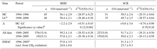
Notes: Values in parentheses are the number of outliers (mild/extreme; see the footnote 4); the latter were excluded from the calculation of the long-term (up to 2005) averages. Quoted are standard errors of quasi-annual averages (±1σ). a Time-interpolated value is used for February (no samples are available at SCB during the LC period). b The p value is estimated for the null hypothesis that Δ of δ13C(CO) QAA is below (left-tail test). c The aggregate of the emission inventories used in the simulation correspond closest to 2000 (see details in Gromov et al., 2017).

Figure 1Statistics on the CH4 and CO mixing and 13C ∕ 12C ratios observed at Baring Head (BHD) and Scott Base (SCB) throughout the high-Cl (HC, orange shaded) and low-Cl (LC, grey shaded) periods hypothesised by Allan et al. (2007) (see text for details). Panels (c, d) show statistics on the anomalies with respect to the annual averages (denoted with “Δyr”). Panel (g) displays the number of samples in each subset. The full time series of the data are shown in the Supplement (Fig. S2). Boxes and whiskers present the median and interquartile ranges and ±1σ (of the population) of the data. Circles and minus symbols denote the averages and samples falling outside ±1σ. Solid boxes denote the subset of data when CH4 and CO samples were taken simultaneously (up to 7 days apart); hatched boxes refer to all data.
2.3 EMAC model
For extending the interpretation of observed ETSH CO, we resort to the results of simulations performed with the ECHAM5/MESSy Atmospheric Chemistry (EMAC) general circulation model (Jöckel et al., 2010). EMAC includes all relevant processes (atmospheric transport, calculation of chemistry kinetics, photolysis rates, trace gas emissions, etc.) for simulating the current global atmospheric state. The set-up we use resembles that of the EMAC evaluation study (MESSy Development Cycle 2, Jöckel et al., 2010) and is augmented with kinetic tagging tools (Gromov et al., 2010). These allow direct quantification of the CO component stemming from CH4 oxidation (and as corollary provide λ) by following the carbon (C) exchanges through all intermediates (shown in Supplement Fig. S1) within a comprehensive chemistry mechanism simulated by the MECCA sub-model (Module Efficiently Calculating the Chemistry of the Atmosphere, Sander et al., 2011a). The emission set-up contains only the standard emissions and precursors of Cl and yields average MBL Cl concentrations in the order of 101–102 atoms cm−3 (see the detailed simulated budgets in the Supplement, Table S1). These results are in line with MBL [Cl] of (0.5–2) × 102 atoms cm−3 obtained by Hossaini et al. (2016) in a similar model set-up (ORG2).
The QAAs of [CO] simulated in EMAC for the period 1996–2005 in the grid boxes enclosing the locations of BHD and SCB are also given in Table 1. Despite the spatial and temporal averaging used (∼ 2.8∘ horizontal grid cell size at the T42L31ECMWF resolution, weekly averages), model QAAs match observations well and have similar uncertainties (resulting from monthly means variation; the observed and simulated seasonalities are shown in the Supplement, Fig. S3). Due to longer lifetimes of CO and CH4 in the well-mixed ETSH and, more importantly, their synchronous sink and production via OH, we expect much lower (factor ∼ 1∕5 compared to that of the total CO) variation in the CH4-derived [CO] component. The fraction of the latter (denoted γ, see Table 2) is proportional to the average tropospheric λ of 93 % (diagnosed simulated value). Depending on the zonal domain, Cl atoms in EMAC initiate (0.15–0.25) % of CH4 sink in the troposphere. The fraction of CH4 removed in the ETSH (43 Tg(C) yr−1) is minor compared to that in the tropics (271 Tg(C) yr−1). About 13 % of tropospheric sink occurs in the boundary layer.
Additionally, we simulate the sink-effective 13C enrichment in CO (denoted ηc) resulting from the 12C-preferential CO + OH reaction and removal of the CH4 → CO chain intermediates (dry or wet deposition, when γ < 1), convoluted with atmospheric mixing and transport. The corresponding ηc value at a given space–time point denotes how much higher the δ13C of airborne CO is compared to the case when sink KIEs were absent5. Altogether, values of γ and ηc at the stations and domain-wise integrals of CH4 sink (S) and λ (listed in Table 2) are used in the calculations that follow now.
2.4 Sensitivity of δ13C(CO) to the CH4 + Cl sink
Using the observational and model data, we attempt to estimate the sensitivity of δ13C(CO) at a given station to supposed inter-annual changes in the Cl-initiated CH4 sink. The QAA of δ13C(CO) (denoted δc) can be approximated as a two-component mixture of CH4- and non-CH4-derived CO sources augmented by the effective sink enrichment:
We refer the reader to Table 2 for the explanation of the parameters and their values. In essence, we account for the fractionations induced in atmospheric sinks (ηc in CO and εm in CH4) and mix the sources in the proportion defined by γ. Exemplifying the estimate from A07, SH Cl changes should cause εm to drop from 15 ‰ to 7 ‰ between the HC and LC, rendering δ13C of the carbon from CH4 arriving to CO of −62.2 ‰ and −54.2 ‰, respectively. By rearranging Eq. (1) we derive the non-CH4 CO source δ13C signature δn (see Table 2). Since there are virtually no surface sources of CO south of 40∘ S in the ETSH (see, for example, Gromov et al., 2017, Sect. 3.4), the difference in δn at BHD and SCB could be driven only by poleward 13C enrichment of the non-CH4 in situ sources (e.g. oxidation of higher hydrocarbons) and/or a stronger (than simulated in EMAC) zonal gradient in ηc. Note that the station-wise δn discrepancy scales with the εm value, although not strongly: at εm of OH sink KIE (3.9 ‰) it reduces from (2.2 ± 2.1) ‰ to (1.5 ± 2.2) ‰. In a statistical sense, the derived δn values reflect the same underlying source signature (p value is 0.31).
Table 2Parameters used in calculus.
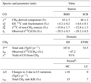
Notes: Quoted QAAs and standard errors (±1σ); the latter are omitted for the components contributing to δc and δn errors insignificantly. a Estimate based on EMAC results. b Derived at εm= 11 ‰ (average of the LC and HC periods). c Includes the LC Cl sink term from A07 (9.7 Tg(C) yr−1). For the SH, the sum of the ETSH and halved intra-tropical integrals is taken. d Estimates from A07.
Using Eq. (1) to define δc in the HC and LC periods, one obtains its sensitivity (Δδc) to changes in the CH4 + Cl sink (ΔS) and in the total sink KIE (Δεm)6:
Here superscripts indicate the period the values are taken for, Δ denotes the HC − LC difference (same as in Sect. 2.2 above) and is the change in the total CH4 sink S relative to the LC conditions. The value of S represents the tropospheric column of a given domain, i.e. we assume that ΔS is distributed homogeneously over the SH or ETSH. Formulated using γ, Eq. (2) allows the projection of the results for the alternative CO yield value λa (different from that obtained in EMAC), as our simulations confirm that λ directly proportionates γ and S in the tropospheric column (but not in the MBL). Furthermore, Δδc is derived under the assumption of constancy of ηc and δn values. Whilst for ηc such is likely the case (judging by the very similar observed CO mixing ratios, and hence lifetimes, during HC and LC), for the latter an upper limit of ±1 ‰ can be put from the typical variation in the δ13C of the underlying sources (see Gromov et al., 2017, Table 5). This is lower than the uncertainty associated with δn values derived here (cf. Table 2); we discuss the range of δn values required to concomitantly mask the changes in δc below.

Figure 2(a) Top: expected CH4 + Cl sink-driven changes to δ13C(CO) between HC and LC periods at the ETSH stations (Δδc) as a function of CH4-derived CO fraction (γ, top axis) resulting from assumed yield values (λa, bottom axis, approximate). Large symbols denote the observed (ordinate) and simulated (abscissa, EMAC) values. Thick lines present Δδc values calculated using Eq. (2) assuming that hypothesised changes to the CH4 + Cl sink occur within the entire SH (solid) and ETSH only (dashed). Thin dashed–dotted lines exemplify the effect due to mere changes in CH4 sink KIE (Δεm). Bottom: average augmentation to the non-CH4 sources signature (Δδn) required to compensate Δδc at the respective values and domains (note the different axis shown in red). Errors bars and areas denote ±1σ of the annual means and derived estimates. See Sects. 2.4 and 3 for details. (b) Tropospheric yield of CO from CH4 oxidation reckoned in the current and previous studies. Symbols (error bars) denote the best (range of) estimates or the global (domain) averages. Abbreviations refer to the following: L81 – Logan et al. (1981), LC91 – Lelieveld and Crutzen (1991), T92 – Tie et al. (1992), M97 – Manning et al. (1997), B00 – Bergamaschi et al. (2000), F06 – Folberth et al. (2006), D07 – Duncan et al. (2007), E10 – Emmons et al. (2010), H11 – Hooghiemstra et al. (2011), G13 – Gromov (2013), GT14 – Gromov and Taraborrelli, MPI-C (unpublished results using EMAC, 2014), F17 – Franco et al. (2018), EMAC – current study.
Figure 2a shows the values of Δδc, calculated for different stations and domains, as a function of γ (implicitly scaling with arbitrarily chosen yield value λa). Very large changes are expected for the ETSH, where μ is about 4 times that in the SH. Importantly, the LCS value includes the Cl sink term from A07 (which is ∼ 29 times greater than the total tropospheric CH4 + Cl sink simulated in EMAC); hence, we receive the “lowest sensitivity” for the case when the Cl sink is added up to (instead of partly replacing) the other CH4 sinks, e.g. that via OH. Alternatively, Δδc will additionally intensify by −0.2 ‰ and −(1.8–2.1) ‰ in the SH and ETSH, respectively. By setting μ= 0 in Eq. (2), we quantify the contribution of the CH4 sink KIE (which increases by Δεm) only. Independent from the assumptions on the Cl sink domain and magnitude, it demonstrates the effect of lowering of δ13C of C arriving to CO from CH4 and accounts for one-third to two-thirds of the total Δδc value (cf. Fig. 2, thin dashed–dotted line).
Finally, we estimate the equivalent increase in the δ13C value of the non-CH4 sources (Δδn) that would be required to mask the depleting effect of a hypothetical CH4 + Cl sink increase. We subtract Eq. (1) written for the HC and LC and solve it assuming Δδc= 0 (notation from Eq. 2 is kept):
Averages of Δδn at BHD and SCB are plotted in the lower panel of Fig. 2a, respectively. Similar to Δδc, Δδn scales with the assumed domain and CH4 input to CO, albeit stronger, because δn is closer to the δ13C of the total CO source (δc−ηc) compared to that for CH4 (δm−εm). Thus, if we accept the EMAC-suggested tropospheric CO yield in the SH of λ= 93 %, Cl-driven changes to the δ13C(CO) at BHD and SCB are expected to be of at least −(5.8–6.3) ‰ between the LC and HC, unless these are masked by unrealistic concurrent increases in δ13C of the non-CH4 sources of about +(11.6–13.5) ‰. If one assumes the CH4 + Cl sink changes only within the ETSH, these estimates scale to −(13.1–14.5) ‰ and +(46–61) ‰, respectively. It is important to note that we gauge the expected changes to the annual averages of δ13C(CO), which do integrate seasonal variations. The latter are observed at merely ±1.5 ‰ (cf. Figs. 1 and S2) and should also increase strongly, if the Cl sink has a similar seasonal variation to that of OH (although A07 used a seasonal cycle based on dimethyl-sulfide-related species in the SH, which has a shorter summer maximum).
The photochemical yield of CO from CH4 constitutes a major factor of uncertainty in the CO budget. Modelling studies to date agreed on values of λ≥ 0.7 (see the overview in Fig. 2b). Several recent studies (see D07, E10 and H11) suggest, however, that λ is close to unity and by doing so contradict findings of 13CO-inclusive studies (see M97, B00 and G13). Assuming that λ < 0.7 or that λ ∼ 1 would be in conflict with basic principles, i.e. photochemical kinetics and dry and wet removal processes affecting the intermediates of the CH4 → CO chain, or their erroneous implementation in the global atmospheric models.
Our estimates of Δδc bear the uncertainty of the assumed λ value; nonetheless, they affirm that even if only 70 % of reacted CH4 molecules yield CO, at least one-third of the changes to the δ13C signature of this source (that is, (δm+εm) times 0.7) should be expressed in the ETSH δ13C(CO). Since δm changed by about +0.1 ‰ between the HC and LC periods (cf. Fig. 1b), we conclude that εm could not change by more than +2 ‰ in the SH as well (with this estimate being lower for λ above 0.7)7. Furthermore, statistically significant non-zero Δδc values (p value of 0.01) should appear at very low λ, viz. above 0.05 (ETSH sink) and 0.12 (SH sink, respectively). We regard these two atmospheric domains because observations in the well-mixed ETSH may not single out the actual location of the Cl + CH4 sink: The large part of sink-driven variations in the mixing ratio and δ13C of CH4 and CO is merely transported into the ETSH from the tropics, where almost three-quarters of the total CH4 sink and accompanying CO production is expected (see Table S1 for EMAC results, also Gromov, 2013, Sect. 6.2.3). Accordingly, Hossaini et al. (2016) also assign a major fraction of the CH4 + Cl sink to the lower latitudes. If such were not the case (i.e. if varying Cl + CH4 sink were confined to the ETSH), the estimated effect on δ13C(CO) would be roughly twice that reckoned for the SH, i.e. extreme values.
There are a few remarks on the usability of the method used by A07, in addition to the thorough theoretical enquiry by Lassey et al. (2011). Evidence, or at least indications, for Cl in the ETSH is based on the [CH4] vs. δ13C(CH4) Lissajous (a.k.a. phase) diagrams being ellipses in the case of seasonal cycles. The slope of their major axis gives the “apparent” KIE, from which the ratio Cl ∕ OH can be inferred when the individual KIEs are known. Clearly, Cl was not assessed on the basis of the annual average value of δ13C(CH4) but on the basis of its seasonal cycle, which is small. Using annual averages, however, is still impeded by perceptible long-term trends in [CH4] and δ13C(CH4), which neither A07 (who consider the final 8 equilibrated years of the 40-year spin-up simulations) nor Lassey et al. (2011) (who use a rather idealised model) have accounted for. For example, presence and asynchronous evolution of [CH4] and δ13C(CH4) long-term trends could result in different mixing and transport of CH4 isotopologues compared to that resulting from trend-free simulated seasonal variations. We note that while observed [CH4] growth is similar throughout both HC and LC periods, such is not the case for δ13C(CH4), which does not increase in the LC (cf. Fig. S2a, c and, in particular, the seasonal time series fits for CH4 at the NIWA website8). Furthermore, the latter is likely a global signal of the 2000–2007 intermittent stop in tropospheric CH4 growth, which manifested itself in δ13C earlier than in mixing ratios and terminated with the reversed 13C ∕ 12C trend (see, for example, Nisbet et al., 2016). Currently available observational data do not allow unambiguous attribution of this global phenomenon to one or several causes proposed (Turner et al., 2017), however.
Our incomplete information about the 13C isotopic composition of CH4 sources presently prevents a Cl-induced input into the annual average value of δ13C(CH4) being singled out, even though it should be perceptible (about +1.5 ‰, assuming for the sake of matter a 2.5 % Cl sink). The corresponding negative shift in δ13C(CO) is about 1.6 ‰ (estimated in Sect. 2.1). In this respect, δ13C(CH4) and δ13C(CO) are equally sensitive to Cl. Because oxidation of CH4 is a main source of CO in the ETSH, and the isotopic composition of atmospheric CH4 is better known than that of its sources, it may well be that variation in the annual average value of δ13C(CO) is a more useful variable for estimating [Cl]. The relatively long lifetime and small seasonality in sources result in weak seasonal cycles of mixing ratio and δ13C in CH4. In contrast, the seasonal cycle of δ13C(CO) is dominated by the large difference in isotopic composition of its sources, with the main driver being the switch between CO from CH4 oxidation and that of the other sources. Since the presence of Cl makes CH4 oxidation an even more 13C-depleted source, the impact of CH4 oxidation on CO in the ETSH peaks and may render the seasonal amplitude (in particular summer minima) of δ13C(CO) a sensitive indicator for Cl. Unfortunately, deficit of observational data (large uncertainties due to insufficient statistics) currently hinder such application.
A fundamental problem remains that the ETSH δ13C(CO) budget cannot be closed even when a Cl sink is excluded, unless a CO yield from CH4 of 0.7–0.86 is assumed (Manning et al., 1997; Bergamaschi et al., 2000). Yields below unity leave, however, the possibility that a positive fractionation in the removal of the CH4 → CO intermediates may be at play. Using λ= (0.7–0.86) and γ= 0.3 for the troposphere, one calculates that an average KIE of (11–33) ‰ should escort the removal of intermediates in order to offset the Cl input to δ13C(CO). This estimate is 3–8 times higher than current parameterisations suggest (about 4 ‰, see Gromov, 2013, Sect. 6.2.4) and is even higher in the SH, where γ is above 0.4. Another complication is potentially present because one cannot exclude that the room temperature laboratory data for the 13C KIE for CO+OH reaction are not applicable to the bulk of the troposphere, even though the reaction itself is little temperature- but mostly pressure-dependent (see Gromov, 2013, Sect. 6.1.4). The unbalanced 13C(CO) budget may then be the consequence of underestimating the CO sink KIE in the models, despite adequate estimates of the sources' 13C ∕ 12C ratios.
We emphasise the value of long-term observations of CO isotopic composition, especially at locations like Scott Base (Antarctica), where influence of local sources is smallest and the fraction of photochemically produced CO is largest. In combination with modelling (e.g. EMAC), δ13C(CO) allows monitoring for intra-annual changes in the carbon isotopic composition of CH4-derived CO, namely the δ13C value of reacted CH4 modified by the total sink KIE (εm). Within the range of probable λ values (0.7–0.93), we are able to cap the potential changes in εm by +(2.0–1.5) ‰ between 1994–1996 and 1998–2000 in the ETSH, which contrasts the +8 ‰ derived by Allan et al. (2007). Conversely, δ13C(CO) may also be employed for “top-down” estimates of δ13C values of CH4 sources, provided the εm is equilibrated on a scale of a tropospheric CH4 lifetime. This could be achieved in a differential mixing model (also known as the “Keeling” plot) contrasting small variance in CH4-derived [CO] and δ13C and largely varying input from other CO sources (e.g. biomass burning).
We conclude that δ13C(CO) is particularly sensitive to the CH4 + Cl sink. Its temporal variations, if they exist, may allow an independent “bottom-up” [Cl] proxy to be calibrated, e.g. emissions of Cl simulated in process-based models. For example, changes in observed δ13C(CO) at SCB (see Table 1) allow variations of the Cl-driven sink of CH4 not larger than (1.5 % of its total (assuming the yield λa of CO from CH4). Projecting this figure onto EMAC results (Table S1, zonal tropospheric integrals) implies that variations in mean ETSH chlorine abundance should have not exceeded Δ[Cl] = (0.9 atoms cm−3 between 1994–1996 and 1998–2000. Regarding the fact that Manning et al. (1997) and Bergamaschi et al. (2000) could only close the SH 13C(CO) budget assuming λ values of 0.7 and 0.86, which are within the generally accepted range, it is unlikely that tropospheric Cl is as high as assumed in the literature.
Although invoking isotopic information is often like opening a can of worms (scientists' favourite diet), relevant conclusions emerge. Lassey et al. (2011) exposed shortcomings of the phase diagram method; we show here, using a low- and high-Cl scenario, that unrealistic yield values of CO from CH4 oxidation (λ below 0.12 in the SH) and/or implausible increases in the δ13C of non-CH4 sources of CO (exceeding +7 ‰ at realistic λ≥ 0.7) would have to be assumed to explain the absence of concurrent inter-annual variations in δ13C(CO) in the ETSH. This constitutes an independent, observation-based evaluation of [Cl] variations envisaged by Allan et al. (2007), from which we conclude that such variations are extremely unlikely. Concerning estimates of background levels of Cl, even attributing 1 % of the total tropospheric sink of CH4 to Cl aggravates the non-trivial problem of balancing the global 13C(CO) budget. It follows that the role of tropospheric Cl as a sink of CH4 oxidation (see, for example, Saunois et al., 2016, and references therein) is seriously overestimated.
The Modular Earth Submodel System (MESSy) is continuously further developed and applied by a consortium of institutions. The usage of MESSy (including the EMAC model) and access to the source code is licensed to all affiliates of institutions which are members of the MESSy Consortium. Institutions can become a member of the MESSy Consortium by signing the MESSy Memorandum of Understanding. Visit the MESSy Consortium website (http://www.messy-interface.org, last access: 27 September 2017) for more information.
Below we detail the derivation of Eqs. (2) and (3). The former is obtained by writing Eq. (1) for the HC and LC periods.
and subtracting these to yield the respective change to δc:
Note that γ is proportional to the product (λ⋅S) and hence increases by (1 + ΔS ∕ LCS) during the HC period. Thus, using
and factoring with respect to LCγ, one obtains:
Finally, the value of Δδc can be projected for any arbitrary yield value λa (different to λ obtained in EMAC and used in our calculations) by scaling the value of LCγ with λa ∕ λ, which yields Eq. (2).
Derivation of Eq. (3) is done in a similar fashion, i.e. equating the right-hand sides of Eq. (1) written for HC and LC periods (assuming that δc does not change):
Rearranging the above expression for Δδn (required change in δn sought) and factoring with respect to LCγ yields the following:
where LCγ can be further modulated by λa ∕ λ to account for an arbitrary yield value, as shown in Eq. (3).
The supplement related to this article is available online at: https://doi.org/10.5194/acp-18-9831-2018-supplement.
The authors declare that they have no conflict of interest.
We are indebted to Martin Manning and the anonymous referee whose expertise and valuable input led to significant improvement of this paper. We thank Taku Umezawa, Sander Houweling and Martin Heimann for discussions on the isotopic composition of CH4. The unique long-term trace gas records from Baring Head (New Zealand) and Scott Base (Antarctica) made available by National Institute of Water and Atmospheric Research (NIWA, 2010) are of great value. We also thank Roland Eichinger for useful comments during the paper preparation.
This work was supported by German Federal Ministry of Education and Research
(BMBF) as a Research for Sustainability initiative (FONA,
http://www.fona.de, last access: 16 March 2018) through the PalMod
project (FKZ: 01LP1507A).
The article
processing charges for this open-access
publication were
covered by the Max Planck Society.
Edited by:
Martin Heimann
Reviewed by: Martin Manning and one anonymous
referee
Allan, W., Manning, M. R., Lassey, K. R., Lowe, D. C., and Gomez, A. J.: Modeling the variation of δ13C in atmospheric methane: Phase ellipses and the kinetic isotope effect, Global Biogeochem. Cy., 15, 467–481, https://doi.org/10.1029/2000gb001282, 2001.
Allan, W., Struthers, H., and Lowe, D. C.: Methane carbon isotope effects caused by atomic chlorine in the marine boundary layer: Global model results compared with Southern Hemisphere measurements, J. Geophys. Res.-Atmos., 112, D04306, https://doi.org/10.1029/2006jd007369, 2007.
Baker, A. K., Rauthe-Schöch, A., Schuck, T. J., Brenninkmeijer, C. A. M., van Velthoven, P. F. J., Wisher, A., and Oram, D. E.: Investigation of chlorine radical chemistry in the Eyjafjallajökull volcanic plume using observed depletions in non-methane hydrocarbons, Geophys. Res. Lett., 38, L13801, https://doi.org/10.1029/2011GL047571, 2011.
Baker, A. K., Sauvage, C., Thorenz, U. R., van Velthoven, P., Oram, D. E., Zahn, A., Brenninkmeijer, C. A. M., and Williams, J.: Evidence for strong, widespread chlorine radical chemistry associated with pollution outflow from continental Asia, Sci. Rep., 6, 36821, https://doi.org/10.1038/srep36821, 2016.
Bergamaschi, P., Hein, R., Brenninkmeijer, C. A. M., and Crutzen, P. J.: Inverse modeling of the global CO cycle 2. Inversion of 13C ∕ 12C and 18O ∕ 16O isotope ratios, J. Geophys. Res.-Atmos., 105, 1929–1945, https://doi.org/10.1029/1999jd900819, 2000.
Brenninkmeijer, C. A. M.: Measurement of the abundance of 14CO in the atmosphere and the 13C ∕ 12C and 18O ∕ 16O ratio of atmospheric CO with applications in New Zealand and Antarctica, J. Geophys. Res.-Atmos., 98, 10595–10614, https://doi.org/10.1029/93JD00587, 1993.
Brenninkmeijer, C. A. M., Müller, R., Crutzen, P. J., Lowe, D. C., Manning, M. R., Sparks, R. J., and van Velthoven, P. F. J.: A large 13CO deficit in the lower Antarctic stratosphere due to “Ozone Hole” Chemistry: Part I, Observations, Geophys. Res. Lett., 23, 2125–2128, https://doi.org/10.1029/96gl01471, 1996.
Craig, H.: Isotopic standards for carbon and oxygen and correction factors for mass-spectrometric analysis of carbon dioxide, Geochim. Cosmochim. Ac., 12, 133–149, https://doi.org/10.1016/0016-7037(57)90024-8, 1957.
Crowley, J. N., Saueressig, G., Bergamaschi, P., Fischer, H., and Harris, G. W.: Carbon kinetic isotope effect in the reaction CH4 + Cl: a relative rate study using FTIR spectroscopy, Chem. Phys. Lett., 303, 268–274, https://doi.org/10.1016/S0009-2614(99)00243-2, 1999.
Duncan, B. N., Logan, J. A., Bey, I., Megretskaia, I. A., Yantosca, R. M., Novelli, P. C., Jones, N. B., and Rinsland, C. P.: Global budget of CO, 1988–1997: Source estimates and validation with a global model, J. Geophys. Res.-Atmos., 112, D22301, https://doi.org/10.1029/2007jd008459, 2007.
Emmons, L. K., Walters, S., Hess, P. G., Lamarque, J.-F., Pfister, G. G., Fillmore, D., Granier, C., Guenther, A., Kinnison, D., Laepple, T., Orlando, J., Tie, X., Tyndall, G., Wiedinmyer, C., Baughcum, S. L., and Kloster, S.: Description and evaluation of the Model for Ozone and Related chemical Tracers, version 4 (MOZART-4), Geosci. Model Dev., 3, 43–67, https://doi.org/10.5194/gmd-3-43-2010, 2010.
Folberth, G. A., Hauglustaine, D. A., Lathière, J., and Brocheton, F.: Interactive chemistry in the Laboratoire de Météorologie Dynamique general circulation model: model description and impact analysis of biogenic hydrocarbons on tropospheric chemistry, Atmos. Chem. Phys., 6, 2273–2319, https://doi.org/10.5194/acp-6-2273-2006, 2006.
Franco, B., Taraborrelli, D., Gromov, S., Pozzer, A., Clarisse, L., Coheur, P.-F., Mahieu, E., Lumenstock, T., Clerbaux, C., De Mazière, M., De Smedt, I., Griffith, D. W. T., Hannigan, J. W., Hase, F., Jones, N., Lutsch, E., Ortega, I., Paton-Walsh, C., Pommier, M., Sander, R., Schneider, M., Strong, K., Van Roozendael, M., Vigouroux, C., Kiendler-Scharr, A., and Wahner, A.: Ubiquitous production of organic acids mediated by warm clouds, in review, 2018.
Gromov, S., Jöckel, P., Sander, R., and Brenninkmeijer, C. A. M.: A kinetic chemistry tagging technique and its application to modelling the stable isotopic composition of atmospheric trace gases, Geosci. Model Dev., 3, 337–364, https://doi.org/10.5194/gmd-3-337-2010, 2010.
Gromov, S., Brenninkmeijer, C. A. M., and Jöckel, P.: Uncertainties of fluxes and 13C ∕ 12C ratios of atmospheric reactive-gas emissions, Atmos. Chem. Phys., 17, 8525–8552, https://doi.org/10.5194/acp-17-8525-2017, 2017.
Gromov, S. S.: Stable isotope composition of atmospheric carbon monoxide: A modelling study, Johannes Gutenberg-Universität, Mainz, urn:urn:nbn:de:hebis:77-37475, available at: http://nbn-resolving.de/urn:nbn:de:hebis:77-37475, 2013.
Hewitt, A. D., Brahan, K. M., Boone, G. D., and Hewitt, S. A.: Kinetics and mechanism of the Cl + CO reaction in air, Int. J. Chem. Kinet., 28, 763–771, https://doi.org/10.1002/(SICI)1097-4601(1996)28:10<763::AID-KIN7>3.0.CO;2-L, 1996.
Hooghiemstra, P. B., Krol, M. C., Meirink, J. F., Bergamaschi, P., van der Werf, G. R., Novelli, P. C., Aben, I., and Röckmann, T.: Optimizing global CO emission estimates using a four-dimensional variational data assimilation system and surface network observations, Atmos. Chem. Phys., 11, 4705–4723, https://doi.org/10.5194/acp-11-4705-2011, 2011.
Hossaini, R., Chipperfield, M. P., Saiz-Lopez, A., Fernandez, R., Monks, S., Feng, W., Brauer, P., and von Glasow, R.: A global model of tropospheric chlorine chemistry: Organic versus inorganic sources and impact on methane oxidation, J. Geophys. Res.-Atmos., 121, 271–214, 297, https://doi.org/10.1002/2016JD025756, 2016.
Jobson, B. T., Niki, H., Yokouchi, Y., Bottenheim, J., Hopper, F., and Leaitch, R.: Measurements of C2–C6 hydrocarbons during the Polar Sunrise1992 Experiment: Evidence for Cl atom and Br atom chemistry, J. Geophys. Res.-Atmos., 99, 25355–25368, https://doi.org/10.1029/94JD01243, 1994.
Jöckel, P., Kerkweg, A., Pozzer, A., Sander, R., Tost, H., Riede, H., Baumgaertner, A., Gromov, S., and Kern, B.: Development cycle 2 of the Modular Earth Submodel System (MESSy2), Geosci. Model Dev., 3, 717–752, https://doi.org/10.5194/gmd-3-717-2010, 2010.
Lassey, K. R., Brailsford, G. W., Bromley, A. M., Martin, R. J., Moss, R. C., Gomez, A. J., Sherlock, V., Allan, W., Nichol, S. E., Schaefer, H., Connor, B. J., Robinson, J., and Smale, D.: Recent changes in methane mixing ratio and its 13C content observed in the southwest Pacific region, J. Integr. Environ. Sci., 7, 109–117, https://doi.org/10.1080/19438151003621441, 2010.
Lassey, K. R., Allan, W., and Fletcher, S. E. M.: Seasonal inter-relationships in atmospheric methane and companion δ13C values: effects of sinks and sources, Tellus B, 63, 287–301, https://doi.org/10.1111/j.1600-0889.2011.00535.x, 2011.
Lelieveld, J. and Crutzen, P. J.: The Role of Clouds in Tropospheric Photochemistry, J. Atmos. Chem., 12, 229–267, https://doi.org/10.1007/BF00048075, 1991.
Lelieveld, J., Gromov, S., Pozzer, A., and Taraborrelli, D.: Global tropospheric hydroxyl distribution, budget and reactivity, Atmos. Chem. Phys., 16, 12477–12493, https://doi.org/10.5194/acp-16-12477-2016, 2016.
Levine, J. G., Wolff, E. W., Jones, A. E., and Sime, L. C.: The role of atomic chlorine in glacial-interglacial changes in the carbon-13 content of atmospheric methane, Geophys. Res. Lett., 38, L04801, https://doi.org/10.1029/2010GL046122, 2011a.
Levine, J. G., Wolff, E. W., Jones, A. E., Sime, L. C., Valdes, P. J., Archibald, A. T., Carver, G. D., Warwick, N. J., and Pyle, J. A.: Reconciling the changes in atmospheric methane sources and sinks between the Last Glacial Maximum and the pre-industrial era, Geophys. Res. Lett., 38, L23804, https://doi.org/10.1029/2011GL049545, 2011b.
Liao, J., Huey, L. G., Liu, Z., Tanner, D. J., Cantrell, C. A., Orlando, J. J., Flocke, F. M., Shepson, P. B., Weinheimer, A. J., Hall, S. R., Ullmann, K., Beine, H. J., Wang, Y., Ingall, E. D., Stephens, C. R., Hornbrook, R. S., Apel, E. C., Riemer, D., Fried, A., Mauldin Iii, R. L., Smith, J. N., Staebler, R. M., Neuman, J. A., and Nowak, J. B.: High levels of molecular chlorine in the Arctic atmosphere, Nat. Geosci., 7 , 91–94, https://doi.org/10.1038/ngeo2046, 2014.
Logan, J. A., Prather, M. J., Wofsy, S. C., and McElroy, M. B.: Tropospheric chemistry: A global perspective, J. Geophys. Res.-Oceans, 86, 7210–7254, https://doi.org/10.1029/JC086iC08p07210, 1981.
Lowe, D. C., Brenninkmeijer, C. A. M., Tyler, S. C., and Dlugkencky, E. J.: Determination of the isotopic composition of atmospheric methane and its application in the Antarctic, J. Geophys. Res.-Atmos., 96, 15455–15467, https://doi.org/10.1029/91JD01119, 1991.
Lowe, D. C., Allan, W., Manning, M. R., Bromley, T., Brailsford, G., Ferretti, D., Gomez, A., Knobben, R., Martin, R., Mei, Z., Moss, R., Koshy, K., and Maata, M.: Shipboard determinations of the distribution of 13C in atmospheric methane in the Pacific, J. Geophys. Res.-Atmos., 104, 26125–26135, https://doi.org/10.1029/1999jd900452, 1999.
Manning, M. R., Brenninkmeijer, C. A. M., and Allan, W.: Atmospheric carbon monoxide budget of the southern hemisphere: Implications of 13C ∕ 12C measurements, J. Geophys. Res.-Atmos., 102, 10673–10682, https://doi.org/10.1029/96JD02743, 1997.
Müller, R., Brenninkmeijer, C. A. M., and Crutzen, P. J.: A Large 13CO deficit in the lower Antarctic stratosphere due to “ozone hole” chemistry: Part II, Modeling, Geophys. Res. Lett., 23, 2129–2132, https://doi.org/10.1029/96gl01472, 1996.
Natrella, M.: NIST/SEMATECH e-Handbook of Statistical Methods, edited by: Croarkin, C. and Tobias, P., NIST/SEMATECH, available at: http://www.itl.nist.gov/div898/handbook/ (last access: 20 August 2015), 2003.
Nisbet, E. G., Dlugokencky, E. J., Manning, M. R., Lowry, D., Fisher, R. E., France, J. L., Michel, S. E., Miller, J. B., White, J. W. C., Vaughn, B., Bousquet, P., Pyle, J. A., Warwick, N. J., Cain, M., Brownlow, R., Zazzeri, G., Lanoisellé, M., Manning, A. C., Gloor, E., Worthy, D. E. J., Brunke, E. G., Labuschagne, C., Wolff, E. W., and Ganesan, A. L.: Rising atmospheric methane: 2007–2014 growth and isotopic shift, Global Biogeochem. Cy., 30, 1356–1370, https://doi.org/10.1002/2016GB005406, 2016.
NIWA: Publicly available data on from several greenhouse gas measurement projects (TROPAC), National Institute of Water and Atmospheric Research, New Zealand, available at: ftp://ftp.niwa.co.nz/tropac/ (last access: 23 June 2016), 2010.
Osthoff, H. D., Roberts, J. M., Ravishankara, A. R., Williams, E. J., Lerner, B. M., Sommariva, R., Bates, T. S., Coffman, D., Quinn, P. K., Dibb, J. E., Stark, H., Burkholder, J. B., Talukdar, R. K., Meagher, J., Fehsenfeld, F. C., and Brown, S. S.: High levels of nitryl chloride in the polluted subtropical marine boundary layer, Nat. Geosci., 1, 324–328, https://doi.org/10.1038/ngeo177, 2008.
Parrish, D. D., Hahn, C. J., Williams, E. J., Norton, R. B., Fehsenfeld, F. C., Singh, H. B., Shetter, J. D., Gandrud, B. W., and Ridley, B. A.: Reply [to Comment on “Indications of photochemical histories of Pacific air masses from measurements of atmospheric trace species at Point Arena, California' by D. D. Parrish et al.”], J. Geophys. Res.-Atmos., 98, 14995–14997, https://doi.org/10.1029/93JD01416, 1993.
Platt, U., Allan, W., and Lowe, D.: Hemispheric average Cl atom concentration from 13C / 12C ratios in atmospheric methane, Atmos. Chem. Phys., 4, 2393–2399, https://doi.org/10.5194/acp-4-2393-2004, 2004.
Röckmann, T., Brenninkmeijer, C. A. M., Crutzen, P. J., and Platt, U.: Short-term variations in the 13C/12C ratio of CO as a measure of Cl activation during tropospheric ozone depletion events in the Arctic, J. Geophys. Res.-Atmos., 104, 1691–1697, https://doi.org/10.1029/1998JD100020, 1999.
Sander, R., Baumgaertner, A., Gromov, S., Harder, H., Jöckel, P., Kerkweg, A., Kubistin, D., Regelin, E., Riede, H., Sandu, A., Taraborrelli, D., Tost, H., and Xie, Z.-Q.: The atmospheric chemistry box model CAABA/MECCA-3.0, Geosci. Model Dev., 4, 373–380, https://doi.org/10.5194/gmd-4-373-2011, 2011a.
Sander, S. P., Friedl, R. R., Abbatt, J. P. D., Barker, J. R., Burkholder, J. B., Golden, D. M., Kolb, C. E., Kurylo, M. J., Moortgat, G. K., Wine, P. H., Huie, R. E., and Orkin, V. L.: Chemical Kinetics and Photochemical Data for Use in Atmospheric Studies, Evaluation No. 17(JPL Publication 10-6), NASA Jet Propulsion Laboratory, Pasadena, CA, 2011b.
Saueressig, G., Bergamaschi, P., Crowley, J. N., Fischer, H., and Harris, G. W.: Carbon kinetic isotope effect in the reaction of CH4 with Cl atoms, Geophys. Res. Lett., 22, 1225–1228, https://doi.org/10.1029/95GL00881, 1995.
Saueressig, G., Crowley, J. N., Bergamaschi, P., Brühl, C., Brenninkmeijer, C. A. M., and Fischer, H.: Carbon 13 and D kinetic isotope effects in the reactions of CH4 with O(1D) and OH: New laboratory measurements and their implications for the isotopic composition of stratospheric methane, J. Geophys. Res.-Atmos., 106, 23127–23138, https://doi.org/10.1029/2000jd000120, 2001.
Saunois, M., Bousquet, P., Poulter, B., Peregon, A., Ciais, P., Canadell, J. G., Dlugokencky, E. J., Etiope, G., Bastviken, D., Houweling, S., Janssens-Maenhout, G., Tubiello, F. N., Castaldi, S., Jackson, R. B., Alexe, M., Arora, V. K., Beerling, D. J., Bergamaschi, P., Blake, D. R., Brailsford, G., Brovkin, V., Bruhwiler, L., Crevoisier, C., Crill, P., Covey, K., Curry, C., Frankenberg, C., Gedney, N., Höglund-Isaksson, L., Ishizawa, M., Ito, A., Joos, F., Kim, H.-S., Kleinen, T., Krummel, P., Lamarque, J.-F., Langenfelds, R., Locatelli, R., Machida, T., Maksyutov, S., McDonald, K. C., Marshall, J., Melton, J. R., Morino, I., Naik, V., O'Doherty, S., Parmentier, F.-J. W., Patra, P. K., Peng, C., Peng, S., Peters, G. P., Pison, I., Prigent, C., Prinn, R., Ramonet, M., Riley, W. J., Saito, M., Santini, M., Schroeder, R., Simpson, I. J., Spahni, R., Steele, P., Takizawa, A., Thornton, B. F., Tian, H., Tohjima, Y., Viovy, N., Voulgarakis, A., van Weele, M., van der Werf, G. R., Weiss, R., Wiedinmyer, C., Wilton, D. J., Wiltshire, A., Worthy, D., Wunch, D., Xu, X., Yoshida, Y., Zhang, B., Zhang, Z., and Zhu, Q.: The global methane budget 2000–2012, Earth Syst. Sci. Data, 8, 697–751, https://doi.org/10.5194/essd-8-697-2016, 2016.
Schaefer, H., Fletcher, S. E. M., Veidt, C., Lassey, K. R., Brailsford, G. W., Bromley, T. M., Dlugokencky, E. J., Michel, S. E., Miller, J. B., Levin, I., Lowe, D. C., Martin, R. J., Vaughn, B. H., and White, J. W. C.: A 21st century shift from fossil-fuel to biogenic methane emissions indicated by 13CH4, Science, 352, 80–84, https://doi.org/10.1126/science.aad2705, 2016.
Spicer, C. W., Chapman, E. G., Finlayson-Pitts, B. J., Plastridge, R. A., Hubbe, J. M., Fast, J. D., and Berkowitz, C. M.: Unexpectedly high concentrations of molecular chlorine in coastal air, Nature, 394, 353–356, https://doi.org/10.1038/28584, 1998.
Thornton, J. A., Kercher, J. P., Riedel, T. P., Wagner, N. L., Cozic, J., Holloway, J. S., Dubé, W. P., Wolfe, G. M., Quinn, P. K., Middlebrook, A. M., Alexander, B., and Brown, S. S.: A large atomic chlorine source inferred from mid-continental reactive nitrogen chemistry, Nature, 464, 271–274, https://doi.org/10.1038/nature08905, 2010.
Tie, X., Jim Kao, C. Y., and Mroz, E. J.: Net yield of OH, CO, and O3 from the oxidation of atmospheric methane, Atmos. Environ. A-Gen., 26, 125–136, https://doi.org/10.1016/0960-1686(92)90265-M, 1992.
Turner, A. J., Frankenberg, C., Wennberg, P. O., and Jacob, D. J.: Ambiguity in the causes for decadal trends in atmospheric methane and hydroxyl, P. Natl. Acad. Sci. USA, 114, 5367–5372, https://doi.org/10.1073/pnas.1616020114, 2017.
Whitehill, A. R., Joelsson, L. M. T., Schmidt, J. A., Wang, D. T., Johnson, M. S., and Ono, S.: Clumped isotope effects during OH and Cl oxidation of methane, Geochim. Cosmochim. Ac., 196, 307–325, https://doi.org/10.1016/j.gca.2016.09.012, 2017.
Young, C. J., Washenfelder, R. A., Roberts, J. M., Mielke, L. H., Osthoff, H. D., Tsai, C., Pikelnaya, O., Stutz, J., Veres, P. R., Cochran, A. K., VandenBoer, T. C., Flynn, J., Grossberg, N., Haman, C. L., Lefer, B., Stark, H., Graus, M., de Gouw, J., Gilman, J. B., Kuster, W. C., and Brown, S. S.: Vertically Resolved Measurements of Nighttime Radical Reservoirs in Los Angeles and Their Contribution to the Urban Radical Budget, Environ. Sci. Technol., 46, 10965–10973, https://doi.org/10.1021/es302206a, 2012.
Hereinafter we report the 13C ∕ 12C ratio as per mil delta values. The δ13C is defined as δ13C = (R ∕ Rst − 1), where R and Rst denote the sample and standard 13C ∕ 12C ratios. We use the VPDB scale with Rst= 11237.2 × 10−6 (Craig, 1957) throughout this paper (for details on choosing this value see Gromov et al., 2017, Appendix A).
see, for example, the synthesis of the CO and CH4 observational data at https://www.esrl.noaa.gov/gmd/ccgg/gallery/figures/ and references provided therein (last access: 25 November 2017).
Sample collection takes place at the designated clean air site Arrival Heights; some of the NIWA datasets use the abbreviation “AHT” for this site.
We follow the conventions from Natrella (2003) for identifying statistically significant outliers in the datasets. Samples with mixing ratios falling outside inner and outer statistical fences of ±1.5 and ±3 interquartile ranges about the median are considered mild and extreme outliers, respectively.
This value is obtained in a sensitivity simulation (e.g. without the KIEs in CO sink and removal of CH4 → CO chain intermediates) and implies linearity (additivity) of atmospheric mixing and transport processes with respect to species δ13C (see details in Gromov, 2013, Sects. 6.2.4–5).
Explicit derivation of this and following equations is shown in Appendix A.
Calculated as (Δδ13C(CO) − 0.1 ‰) ∕ (γ⋅λ) for values at SCB (see Tables 1 and 2).
https://www.niwa.co.nz/atmosphere/our-data/trace-gas-plots/methane (last access: 17 December 2017).