Technical note: Evaluation of the simultaneous measurements of mesospheric OH, HO₂, and O₃ under a photochemical equilibrium assumption – a statistical approach

This Technical Note presents a statistical approach to evaluating simultaneous measurements of several atmospheric components under the assumption of photochemical equilibrium. We consider simultaneous measurements of OH, HO₂, and O₃ at the altitudes of the mesosphere as a specific example and their daytime photochemical equilibrium as an evaluating relationship. A simplified algebraic equation relating local concentrations of these components in the 50–100 km altitude range has been derived. The parameters of the equation are temperature, neutral density, local zenith angle, and the rates of eight reactions. We have performed a one-year simulation of the mesosphere and lower thermosphere using a 3-D chemical-transport model. The simulation shows that the discrepancy between the calculated evolution of the components and the equilibrium value given by the equation does not exceed 3–4 % in the full range of altitudes independent of season or latitude. We have developed a statistical Bayesian evaluation technique for simultaneous measurements of OH, HO₂, and O₃ based on the equilibrium equation taking into account the measurement error. The first results of the application of the technique to MLS/Aura data (Microwave Limb Sounder) are presented in this Technical Note. It has been found that the satellite data of the HO₂ distribution regularly demonstrate lower altitudes of this component's mesospheric maximum. This has also been confirmed by model HO₂ distributions and comparison with offline retrieval of HO₂ from the daily zonal means MLS radiance.

1 Introduction

A prominent feature of atmospheric photochemical systems is the presence of a large number of chemical components with short lifetimes and concentrations close to stable photochemical equilibrium at every instant. The condition of balance between their sources and sinks is described by a system of algebraic equations. This system can be used to determine characteristics of hard-to-measure atmospheric species through other measurable components, evaluate results of remote or in situ measurements, estimate reaction rates usually known with significant uncertainty, and to understand processes and chemical reactions that influence the variability in the most important atmospheric components, e.g., ozone, in the geographical region of interest.

This approach has found the following wide applications:

1. In 3-D chemical transport models that include a large set of physical and chemical processes with a broad spectrum of spatio-temporal scales. In particular, the chemical family concept is widely used for simulating gas-phase photochemistry of the lower and middle atmosphere (e.g., Douglass et al., 1989; Kaye and Rood, 1989; Rasch et al., 1995), when transport is taken into account only for the concentration of a chemical family, while relative concentrations of the constituent fast components are calculated from the instantaneous stable equilibrium condition. Complemented with Henry's law (e.g., Djouad et al., 2003; Tulet et al., 2006) in multiphase models, this approach markedly saves calculation time and increases the overall stability of the numerical scheme. Moreover, use of the photochemical equilibrium condition to simulate fast component dynamics reduces the phase space dimension of box models significantly (e.g., Kulikov and Feigin, 2014), allowing a comprehensive analysis of nontrivial nonlinear dynamic properties of various atmospheric photochemical systems (e.g., Feigin and Konovalov, 1996; Feigin et al., 1998; Konovalov et al., 1999; Konovalov and Feigin, 2000; Kulikov et al., 2012).

2. In investigations of the chemistry of the surface layer and free troposphere in different regions (over megalopolises, in rural areas, in the mountains, over the seas) based on measurements of nitrogen species, peroxy radicals, ozone, aerosols, and other components aimed at understanding processes impacting the surface ozone formation and air quality. The equilibrium condition is most frequently used for nitrogen species. For example, Chameides (1975) proposed a model for determining the vertical distribution of odd nitrogen, in which the HNO₃ profile could be deployed to retrieve profiles of five other components (NO, NO₂, NO₃, N₂O₅, and HNO₂) from their photochemical equilibrium condition. In the paper by Stedman et al. (1975), the equation for NO₂ equilibrium that accounted only for the main source and sink of this component was applied to determine the photodissociation constant J(NO₂). A more accurate equation for the NO₂ equilibrium was used by Crawford et al. (1996) and Koike et al. (1996) to determine NO₂∕NO partitioning and NO_x, allowing for, in particular, an investigation of the spatial distribution of NO_x∕NO_y over the Pacific.

   Nighttime equilibrium in the NO₂-NO₃-N₂O₅ system is used to determine surface layer N₂O₅ concentration, equilibrium constant of this system, equilibrium partitioning between NO₃ and N₂O₅, and loss coefficients of NO₃, N₂O₅, and NO_x (Martinez et al., 2000; Brown et al., 2003; Crowley et al., 2010; McLaren et al., 2010; Benton et al., 2010; Sobanski et al., 2016).

   Platt et al. (1979) used the CH₂O photochemical equilibrium condition to analyze results of simultaneous measurement of CH₂O, O₃, and NO₂ and to identify mechanisms of CH₂O formation over rural areas and in maritime air. In the papers by Ko et al. (2003), Cantrell et al. (2003), and Penkett et al. (1997, 1998) algebraic expressions derived from equilibrium conditions for H₂O₂, peroxy radicals, and nitrogen species were used to determine equilibrium values of peroxide concentration, total peroxy radical level, and NO∕NO₂ ratio, and to diagnose the ozone production and loss levels in a clean or polluted troposphere.

3. In stratospheric chemistry studies, including determination of a critical parameter in catalytic cycles of ozone destruction in the polar stratosphere. In particular, the equilibrium condition for ClO and Cl₂O₂ along with the measurement data of daytime and nighttime concentrations of these components in the polar stratosphere are used to evaluate the temperature dependence of the ClO concentration, reaction constants determining the ClO + ClO + M ↔ Cl₂O₂ + M equilibrium, and the photolysis rate of Cl₂O₂ (Ghosh et al., 1997; Avallone et al., 2001; Solomon et al., 2002; Stimpfle et al., 2004; von Hobe et al., 2005, 2007; Berthet et al., 2005; Butz et al., 2007; Kremser et al., 2011; Sumińska-Ebersoldt et al., 2012; Wetzel et al., 2012).

   Pyle et al. (1983) proposed a method for derivation of the OH concentration from satellite infrared measurements of NO₂ and HNO₃ using a simple algebraic relation following from the equilibrium condition for HNO₃. Algorithms for retrieving distributions of OH and HO₂ from the satellite measurement data of O₃, NO₂, H₂O, HNO₃ by LIMS/Nimbus-7 and UARS with the help of algebraic models following from the photochemical equilibrium of O_x, HO_x, and HNO₃ components were proposed by Pyle and Zavody (1985) and Pickett and Peterson (1996). It is also noteworthy that similar models are widely used for calculating concentrations of components with a short lifetime (e.g., O(¹D) and OH) and subsequently evaluating vertical distributions of eddy diffusivity from measurements of trace gas concentration profiles (e.g., see Massie and Hunten, 1981).

   Kondo et al. (1988) made use of the photochemical equilibrium between NO and NO₂ for understanding diurnal variations in NO concentration measured during aircraft flights. In the paper by Webster et al. (1990) simultaneous in situ balloon-borne measurements of NO, NO₂, HNO₃, O₃, and N₂O and the photochemical equilibrium condition for various nitrogen components were used to determine OH, N₂O₅, and NO_y concentrations. A similar approach was employed by Kawa et al. (1990), who obtained NO₂, N₂O₅, ClNO₃, HNO₃, and OH concentrations from aircraft measurements of NO, ClO, and O₃ concentrations. Hauchecorne et al. (2010) found that NO₃ concentration measured by GOMOS/ENVISAT positively correlates with temperature at altitudes up to 45 km in the region where NO₃ is in chemical equilibrium with O₃. Funke et al. (2005) used NO and NO₂ stable-state photochemistry to verify correctness of the new approach of retrieving distributions of those components from MIPAS/ENVISAT measurement data. Marchand et al. (2007) proposed a method to retrieve the temperature distribution in the stratosphere between 30 and 40 km from O₃ and NO₃ measurements by GOMOS with the help of a simple equation derived from the nighttime NO₃ chemical equilibrium.

4. In investigations of the chemistry of O_x-HO_x components and atmospheric glows in the mesosphere to lower thermosphere (MLT) area. In particular, Kulikov et al. (2006, 2009a) proposed algorithms for the simultaneous retrieval of O, H, HO₂, and H₂O from joint OH and O₃ satellite measurement, in which the assumption of photochemical equilibrium of O₃, OH, and HO₂ was utilized. For several decades the assumption of the photochemical equilibrium of ozone (PEO) was widely used to determine distributions of atomic oxygen and atomic hydrogen at altitudes of the MLT via satellite and rocket measurements of ozone concentration and airglow emissions (e.g., Evans and Llewellyn, 1973; Good, 1976; Pendleton et al., 1983; McDade et al., 1985; McDade and Llewellyn, 1988; Evans et al., 1988; Thomas, 1990; Llewellyn et al., 1993; Llewellyn and McDade, 1996; Mlynczak et al., 2007, 2013a, b, 2014; Smith et al., 2010; Siskind et al., 2008, 2015). Russell and Lowe (2003) applied PEO to infer the seasonal and global climatology of atomic oxygen using WINDII/UARS. PEO was deployed to investigate hydroxyl emission mechanisms, morphology, and variability in the MLT region (Marsh et al., 2006; Xu et al., 2010, 2012; Kowalewski et al., 2014). Mlynczak and Solomon (1991, 1993) and Mlynczak et al. (2013b) used the equilibrium assumption to derive exothermic chemical heat. The PEO assumption was employed for studying the mesospheric OH* layer response to gravity waves (Swenson and Gardner, 1998). In ultimately theoretical works, e.g., Grygalashvyly et al. (2014) and Grygalashvyly (2015), PEO was used to derive the dependence of excited hydroxyl layer concentration and altitude on atomic oxygen and temperature. In the paper by Sonnemann et al. (2015) it was used to analyze annual variations of the OH* layer. Moreover, PEO is frequently applied implicitly, when authors are equating the nighttime loss of ozone in the reaction with atomic hydrogen and production of ozone by a 3-body reaction of molecular and atomic oxygen (e.g., Nikoukar et al., 2007).

In the present Technical Note we demonstrate how the photochemical equilibrium condition of several atmospheric components may be employed to statistically validate data of their simultaneous measurements, particularly in the case when measurement error is large.

We consider the simultaneous photochemical daytime equilibrium of OH, HO₂, and O₃ at the altitudes of the mesosphere. We have derived a simplified algebraic equation

$${\displaystyle }F(\mathrm{OH},{\mathrm{HO}}_{\mathrm{2}},{\mathrm{O}}_{\mathrm{3}})=\mathrm{1},$$

describing the relationship between local concentrations of the components at the altitudes of 50–100 km. The only parameters of the equation are temperature, neutral density, local zenith angle, and constants of eight reactions. A one-year simulation of the mesosphere and lower thermosphere based on a 3-D chemical-transport model shows that the discrepancy between the calculated evolution of the components and the equilibrium value given by the equation does not exceed 3–4 % in the full range of altitudes independent of season or latitude.

We have developed a statistical Bayesian evaluation technique for simultaneous measurement of OH, HO₂, and O₃ based on the mentioned equilibrium equation taking into account the measurement error. The first results of its application to MLS/Aura data (Wang et al., 2015a, b; Schwartz et al., 2015) are presented. It is found that the satellite data of the HO₂ distribution regularly demonstrate lower altitudes of this component's mesospheric maximum. These results confirm the ones obtained via the offline retrieval of HO₂ from the MLS primary data (Millán et al., 2015).

This Technical Note is structured as follows. A 3-D chemical transport model is briefly described in Sect. 2. In Sect. 3, a simplified algebraic relationship between the equilibrium concentrations of OH, HO₂, and O₃ is derived and verified by 3-D simulations. Section 4 presents the method of statistical evaluation of simultaneous data of OH, HO₂, and O₃. The results of applying the method to MLS/Aura data are presented in Sect. 5. The last section contains a discussion of the results followed by concluding remarks.

2 Model and calculations

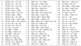
For our calculations we used the global 3-D chemical transport model (CTM) of the middle atmosphere developed by the Leibniz Institute of Atmospheric Physics (IAP; e.g., Berger, 1994; Ebel et al., 1995; Kremp et al., 1999; Berger and von Zahn, 1999; Hartogh et al., 2004, 2011; Sonnemann et al., 1998, 2006, 2007). It was designed particularly for investigation of the spatio-temporal structure of phenomena in the MLT region and specifically in the extended mesopause region. The grid-point model extends from the ground up to the middle thermosphere (0–150 km; 118 pressure-height levels). The horizontal resolution amounts to 5.625^∘ latitudinally and 5.625^∘ longitudinally. The chemical module described in numerous papers (e.g., Sonnemann et al., 1998; Körner and Sonnemann, 2001; Grygalashvyly et al., 2009, 2011, 2012) consists of 19 constituents, 49 chemical reactions, and 14 photo-dissociation reactions (see Table 1). The reaction rates used in the model are taken from Burkholder et al. (2015). The temperature-dependent reaction rates are calculated online; thus, they are sensitive to small temperature fluctuations. We make use of the pre-calculated dissociation rates (Kremp et al., 1999).

Table 1 List of reactions.

The evolution of the components of the HO_x (H, OH, HO₂, H₂O₂) and NO_x (N, NO, NO₂, NO₃) families is calculated using the chemical family concept proposed by Shimazaki (Shimazaki, 1985). This is done because of the presence of short-lived components among these families, with lifetimes much shorter than those of the families themselves, which imposes significant restrictions on the value of the CTM's integration step. For example, the daytime lifetimes of OH and HO₂ above 70 km are about 1 s or less, while the lifetime of the HO_x family is about 10⁴ s or more. Therefore, when calculating these components individually it is necessary to set the CTM's integration step to be much less than 1 s. In our work, the Shimazaki technique is applied for calculating the evolution of each component of the HO_x and NO_x families. We emphasize that this technique does not explicitly use the steady-state approximation for the components, instead it utilizes the approach based on an implicit Euler scheme (see Shimazaki, 1985). This allows for increasing the integration step of the CTM significantly without loss of accuracy in calculating the short-lived components. In our work the integration time is chosen to be 9 s.

The model includes 3-D advective and vertical diffusive transport (turbulent and molecular). Three-dimensional fields of temperature and winds are taken from the Canadian Middle Atmosphere Model (CMAM) for the year 2000 (de Grandpre et al., 2000; Scinocca et al., 2008). We use the Walcek scheme (Walcek and Aleksic, 1998; Walcek, 2000) for advective transport and the implicit Thomas algorithm as described in Morton and Mayers (1994) for diffusive transport. The vertical eddy diffusion coefficient is based on the results by Lübken (1997).

Figure 1 Daytime monthly averaged zonal mean F distributions.

We calculate the annual variation in spatio-temporal distributions of OH, HO₂, and O₃ and constructed distributions of the F(OH, HO₂,O₃) function introduced in Sect. 1. To remove transitional regions that correspond to sunset and sunrise, we only take into account periods of local time with the solar zenith angle χ<85^∘. The obtained results are presented in the model coordinates, so the pressure-height levels are used for the vertical axes. In addition, the approximate altitudes are shown in the figures of Sect. 1, calculated for a given month utilizing averaged temperature profiles of the model and hydrostatic equilibrium.

Figure 2 Daytime monthly averaged zonal mean P_OH distributions (in cm⁻³ s⁻¹).

3 Daytime photochemical equilibrium of OH, HO₂, and O₃ at the altitudes of the mesosphere

The daytime balance of OH concentration at mesospheric altitudes is determined by the following primary reactions (Brasseur and Solomon, 2005):

$$\begin{array}{ll}{\displaystyle }& {\displaystyle }{\mathrm{HO}}_{\mathrm{2}}+\mathrm{O}\to \mathrm{OH}+{\mathrm{O}}_{\mathrm{2}}\left(\mathrm{R}\mathrm{18}\mathrm{in}\mathrm{Table}\mathrm{1}\right),\\ {\displaystyle }& {\displaystyle }\mathrm{H}+{\mathrm{O}}_{\mathrm{3}}\to \mathrm{OH}+{\mathrm{O}}_{\mathrm{2}}\left(\mathrm{R}\mathrm{21}\right),\\ {\displaystyle }& {\displaystyle }\mathrm{H}+{\mathrm{HO}}_{\mathrm{2}}\to \mathrm{2}\mathrm{OH}\left(\mathrm{R}\mathrm{14}\right),\\ {\displaystyle }& {\displaystyle }\mathrm{OH}+\mathrm{O}\to \mathrm{H}+{\mathrm{O}}_{\mathrm{2}}\left(\mathrm{R}\mathrm{17}\right),\\ {\displaystyle }& {\displaystyle }\mathrm{OH}+{\mathrm{O}}_{\mathrm{3}}\to {\mathrm{HO}}_{\mathrm{2}}+{\mathrm{O}}_{\mathrm{2}}\left(\mathrm{R}\mathrm{22}\right).\end{array}$$

The daytime balance of the HO₂ concentration is

$$\begin{array}{ll}{\displaystyle }& {\displaystyle }\mathrm{H}+{\mathrm{O}}_{\mathrm{2}}+M\to {\mathrm{HO}}_{\mathrm{2}}+M,M\mathrm{is}\mathrm{molecule}\mathrm{of}\mathrm{air}\left(\mathrm{R}\mathrm{20}\right),\\ {\displaystyle }& {\displaystyle }\mathrm{OH}+{\mathrm{O}}_{\mathrm{3}}\to {\mathrm{HO}}_{\mathrm{2}}+{\mathrm{O}}_{\mathrm{2}}\left(\mathrm{R}\mathrm{22}\right),\\ {\displaystyle }& {\displaystyle }{\mathrm{HO}}_{\mathrm{2}}+\mathrm{O}\to {\mathrm{O}}_{\mathrm{2}}+\mathrm{OH}\left(\mathrm{R}\mathrm{18}\right).\end{array}$$

The daytime balance of the O₃ concentration is

$$\begin{array}{ll}{\displaystyle }& {\displaystyle }\mathrm{O}+{\mathrm{O}}_{\mathrm{2}}+M\to {\mathrm{O}}_{\mathrm{3}}+M\left(\mathrm{R}\mathrm{12}\right),\\ {\displaystyle }& {\displaystyle }{\mathrm{O}}_{\mathrm{3}}+\mathit{\text{hv}}\to {\mathrm{O}}_{\mathrm{2}}+\mathrm{O}\left(\mathrm{R}\mathrm{52}\right),\\ {\displaystyle }& {\displaystyle }{\mathrm{O}}_{\mathrm{3}}+\mathit{\text{hv}}\to {\mathrm{O}}_{\mathrm{2}}+\mathrm{O}{(}^{\mathrm{1}}\mathrm{D}\left)\right(\mathrm{R}\mathrm{53}),\\ {\displaystyle }& {\displaystyle }{\mathrm{O}}_{\mathrm{3}}+\mathrm{H}\to \mathrm{OH}+{\mathrm{O}}_{\mathrm{2}}\left(\mathrm{R}\mathrm{21}\right).\end{array}$$

Expressions for local concentrations of OH, HO₂, and O₃ in the photochemical equilibrium are written in the form

$$\begin{array}{}\text{(1)}& {\displaystyle }& {\displaystyle }\mathrm{OH}={\displaystyle \frac{k_{\mathrm{18}}\cdot {\mathrm{HO}}_{\mathrm{2}}\cdot \mathrm{O}+\mathrm{2}{k}_{\mathrm{14}}\cdot {\mathrm{HO}}_{\mathrm{2}}\cdot \mathrm{H}+k_{\mathrm{21}}\cdot {\mathrm{O}}_{\mathrm{3}}\cdot \mathrm{H}}{k_{\mathrm{17}}\cdot \mathrm{O}+k_{\mathrm{22}}\cdot {\mathrm{O}}_{\mathrm{3}}}},\text{(2)}& {\displaystyle }& {\displaystyle }{\mathrm{HO}}_{\mathrm{2}}={\displaystyle \frac{k_{\mathrm{20}}\cdot M\cdot {\mathrm{O}}_{\mathrm{2}}\cdot \mathrm{H}+k_{\mathrm{22}}\cdot {\mathrm{O}}_{\mathrm{3}}\cdot \mathrm{OH}}{k_{\mathrm{18}}\cdot \mathrm{O}}},\text{(3)}& {\displaystyle }& {\displaystyle }{\mathrm{O}}_{\mathrm{3}}={\displaystyle \frac{k_{\mathrm{12}}\cdot M\cdot {\mathrm{O}}_{\mathrm{2}}\cdot \mathrm{O}}{k_{\mathrm{52}}+k_{\mathrm{53}}+k_{\mathrm{21}}\cdot \mathrm{H}}},\end{array}$$

where k_i are the corresponding reaction constants from Burkholder et al. (2015).

We eliminate O and H from Eqs. (1)–(3) and derive an expression depending only on OH, HO₂, and O₃.

Figure 3 Daytime monthly averaged zonal mean $P_{\mathrm{OH}}^{{\mathrm{H}}_{\mathrm{2}}\mathrm{O}}/P_{\mathrm{OH}}$ distributions.

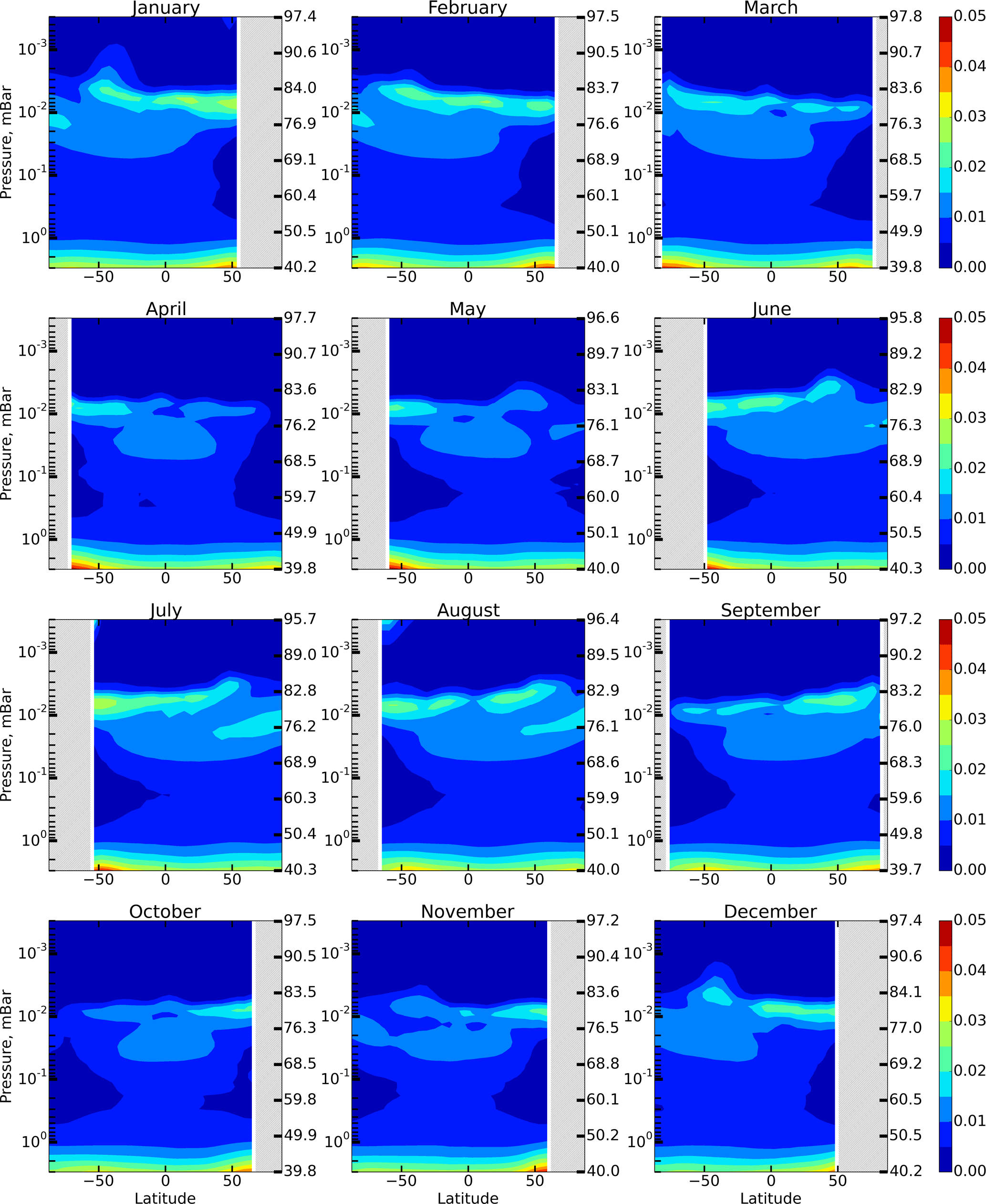
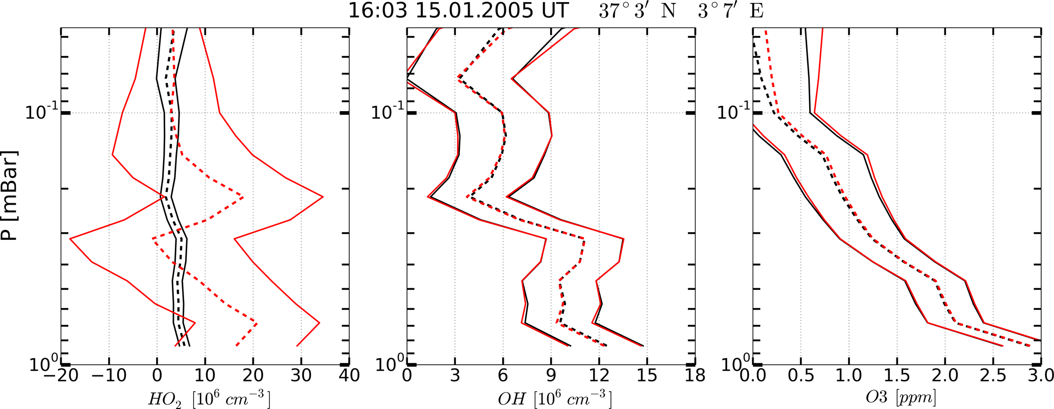
Figure 4 Example of OH, HO₂, and O₃ vertical profiles measured (red curves) on 15 January 2005 at 16:03 UT, 37^∘3^′ N, 3^∘7^′ E and corresponding retrieved profiles (black curves). Solid curves: boundaries of the 65 % confidence intervals, dashed curves: medians.

Almost everywhere in the mesosphere and lower thermosphere (with the exception of 85–95 km, see Kulikov et al., 2017) the photodissociation is the main ozone sink, i.e., $k_{\mathrm{52}}+k_{\mathrm{53}}\gg k_{\mathrm{21}}\cdot \mathrm{H}$. Therefore, in the zero order approximation, Eq. (3) can be simplified and the concentration of atomic oxygen can be defined in terms of ozone concentration:

$$\begin{array}{}\text{(4)}& \mathrm{O}={\displaystyle \frac{k_{\mathrm{52}}+k_{\mathrm{53}}}{k_{\mathrm{12}}\cdot M\cdot {\mathrm{O}}_{\mathrm{2}}}}{\mathrm{O}}_{\mathrm{3}}.\end{array}$$

Making use of Eq. (4) we can derive, from Eq. (2), an expression for the concentration of H in terms of concentrations of OH, HO₂, and O₃:

$$\begin{array}{}\text{(5)}& \mathrm{H}={\displaystyle \frac{k_{\mathrm{18}}\cdot \left(k_{\mathrm{52}}+k_{\mathrm{53}}\right)/\left(k_{\mathrm{12}}\cdot M\cdot {\mathrm{O}}_{\mathrm{2}}\right)\cdot {\mathrm{HO}}_{\mathrm{2}}-k_{\mathrm{22}}\cdot \mathrm{OH}}{k_{\mathrm{20}}\cdot M\cdot {\mathrm{O}}_{\mathrm{2}}}}{\mathrm{O}}_{\mathrm{3}}.\end{array}$$

By substituting this equation and Eq. (4) into Eq. (1) we obtain an expression relating OH, HO₂, and O₃:

$$\begin{array}{ll}{\displaystyle }& {\displaystyle }F\left({\mathrm{OH},\mathrm{HO}}_{\mathrm{2}},{\mathrm{O}}_{\mathrm{3}}\right)\\ {\displaystyle }=& {\displaystyle }\left({\displaystyle \frac{k_{\mathrm{20}}\cdot M\cdot {\mathrm{O}}_{\mathrm{2}}}{k_{\mathrm{20}}\cdot M\cdot {\mathrm{O}}_{\mathrm{2}}+k_{\mathrm{21}}\cdot {\mathrm{O}}_{\mathrm{3}}+\mathrm{2}\cdot k_{\mathrm{14}}\cdot {\mathrm{HO}}_{\mathrm{2}}}}\right.\\ \text{(6)}& {\displaystyle }& {\displaystyle }\left.+{\displaystyle \frac{k_{\mathrm{12}}\cdot M\cdot {\mathrm{O}}_{\mathrm{2}}\cdot k_{\mathrm{22}}}{\left(k_{\mathrm{52}}+k_{\mathrm{53}}\right)\cdot k_{\mathrm{17}}}}\right)\cdot {\displaystyle \frac{k_{\mathrm{17}}\cdot \mathrm{OH}}{k_{\mathrm{18}}\cdot {\mathrm{HO}}_{\mathrm{2}}}}=\mathrm{1}.\end{array}$$

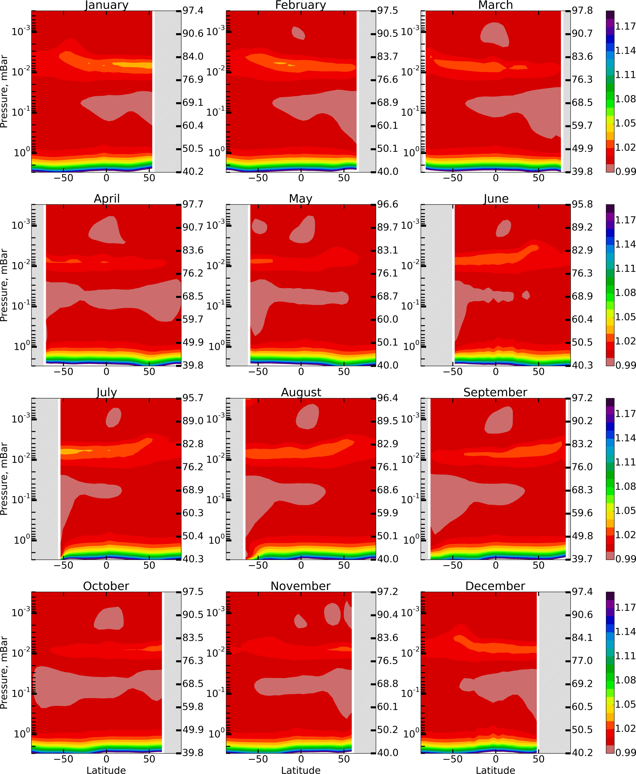
Figure 1 shows height–latitude cross-sections of $\langle F({\mathrm{OH},\mathrm{HO}}_{\mathrm{2}},{\mathrm{O}}_{\mathrm{3}})\rangle$ for each month (in this section angle brackets denote monthly averaged zonal mean values). The gray area corresponds to χ>85^∘. One can see that Eq. (6) is most accurate within the 50–76 km range and above 86 km, where $\left|<F>-\mathrm{1}\right|\le \mathrm{1}$ %. The difference reaches 3–4 % in the region between 76 and 86 km. The altitude of this region has an annual variation with a maximum deviation in the winter hemisphere. Below 50 km the value of $<F>$ increases up to 1.2 at 40 km, thus below the stratopause Eq. (6) no longer describes the simultaneous photochemical equilibrium of OH, HO₂, and O₃. Note that these components remain short-lived below 50 km (with the lifetimes of about 10²–10³ s; Brasseur and Solomon, 2005) depending on height and duration of daylight. However, for a quantitative description of their daytime equilibrium, it is necessary to include additional reactions involving, in particular, the components of the NO_x family.

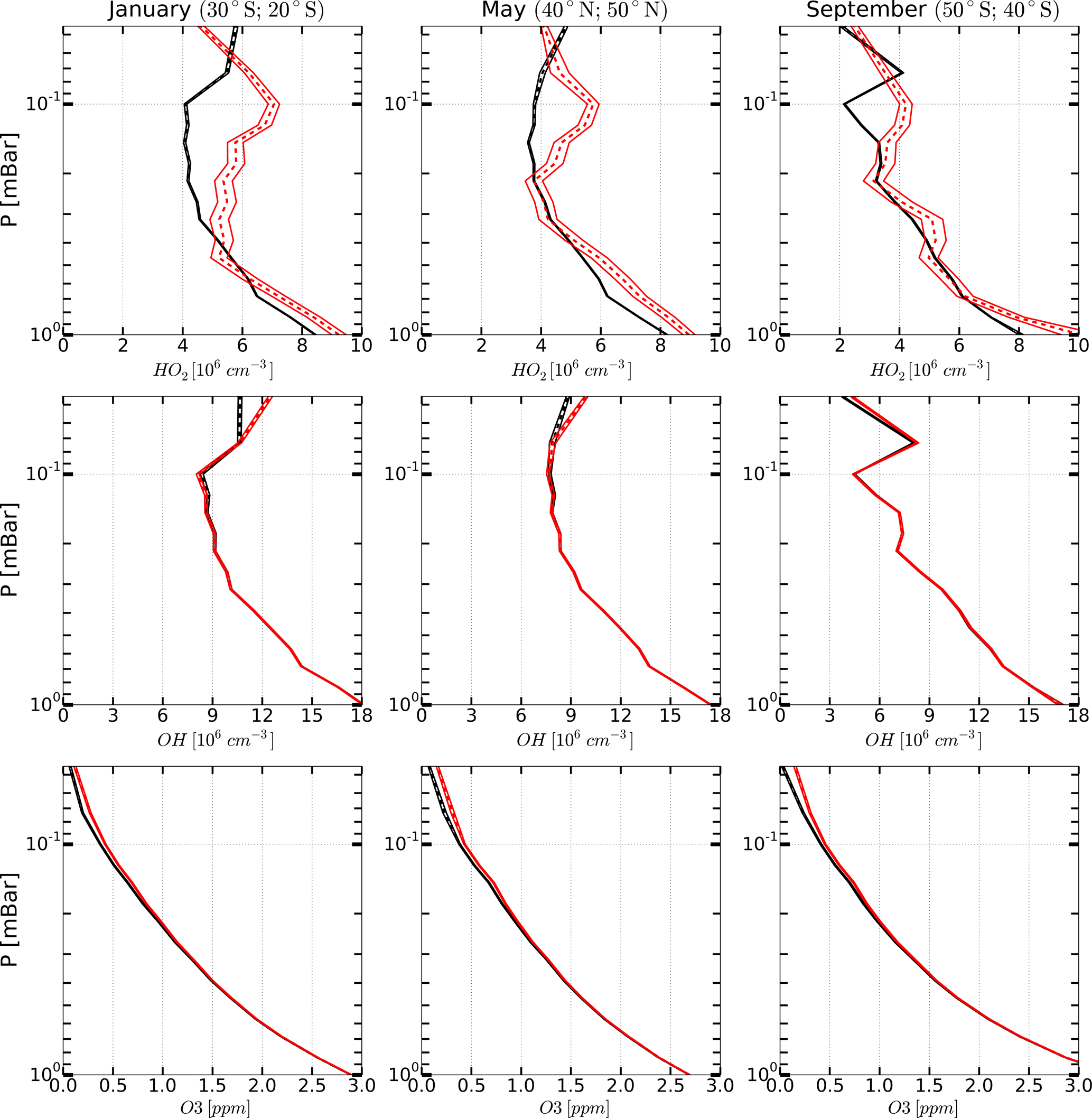
Figure 5 Examples of monthly averaged zonal mean vertical profiles of OH, HO₂, and O₃ measured (red curves) in January, May, and March 2005 and corresponding retrieved profiles (black curves). Solid curves: boundaries of the 65 % confidence intervals, dashed curves: medians.

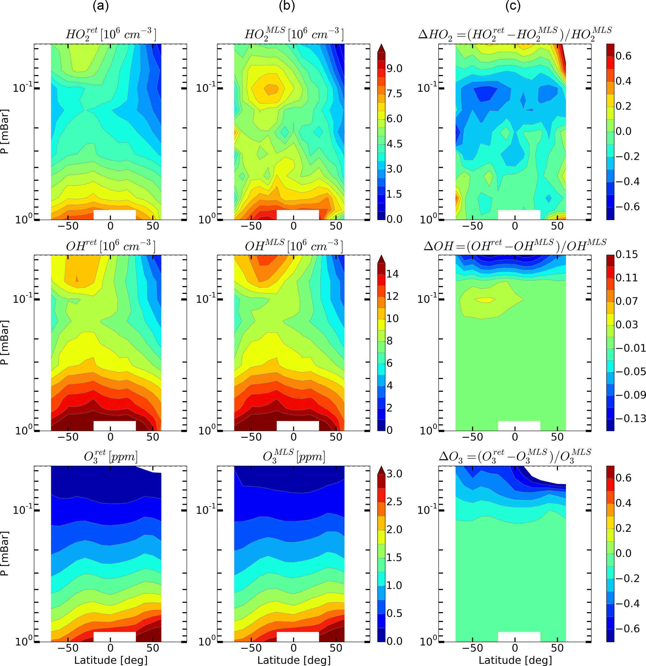
Figure 6 Daytime monthly averaged zonal mean retrieved (a) and measured (b) distributions of HO₂, OH, and O₃ and their relative difference (c) in January 2005.

Figure 7 Daytime monthly averaged zonal mean retrieved (a) and measured (b) distributions of HO₂, OH, and O₃ and their relative difference (c) for May 2005.

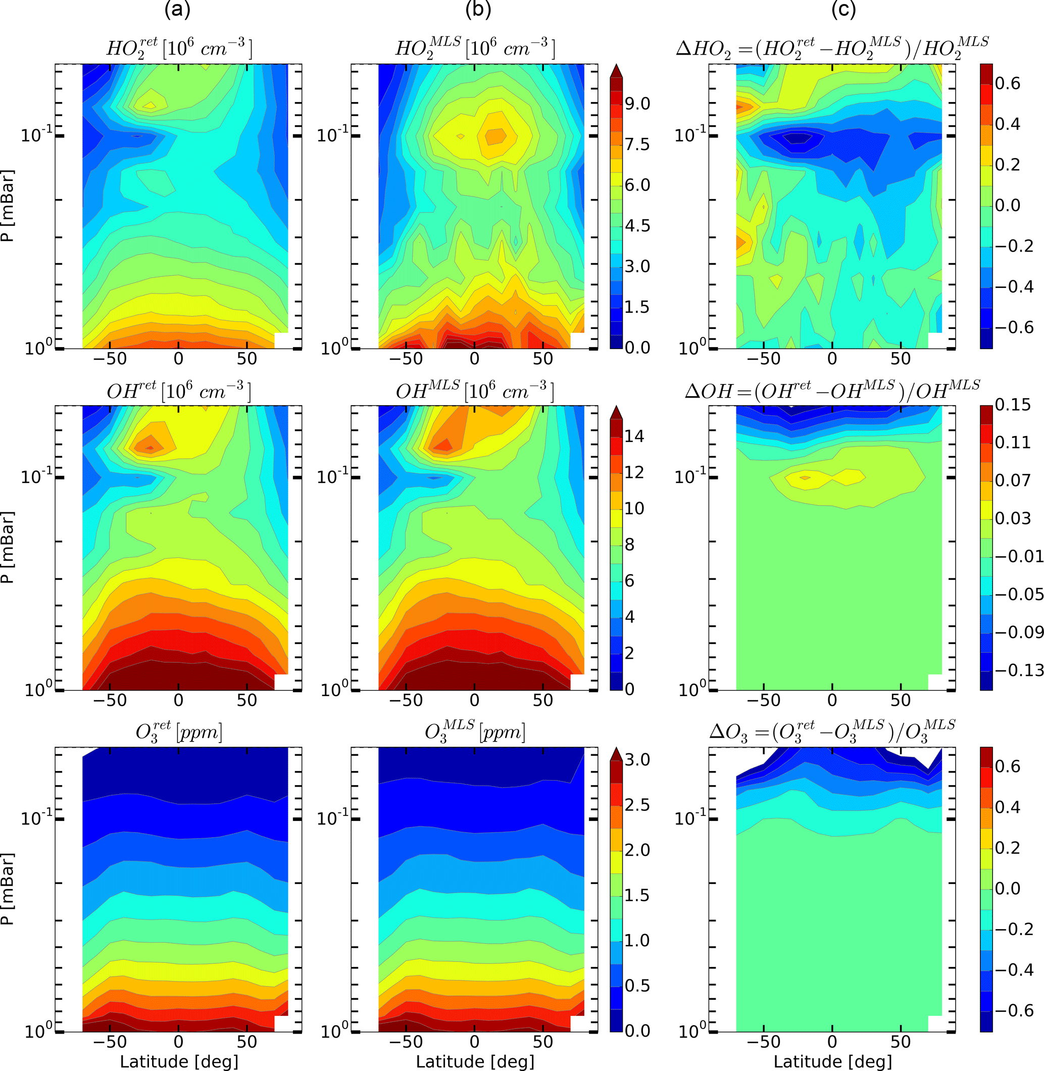
Figure 8 Daytime monthly averaged zonal mean retrieved (a) and measured (b) distributions of HO₂, OH, and O₃ and their relative difference (c) for September 2005.

Note also that Eqs. (1) and (6) take into account only the main daytime source of OH (P_OH) specified by reactions (R18), (R14), and (R21):

$$\begin{array}{}\text{(R1)}& P_{\mathrm{OH}}=k_{\mathrm{18}}\cdot {\mathrm{HO}}_{\mathrm{2}}\cdot \mathrm{O}+\mathrm{2}{k}_{\mathrm{14}}\cdot {\mathrm{HO}}_{\mathrm{2}}\cdot \mathrm{H}+k_{\mathrm{21}}\cdot {\mathrm{O}}_{\mathrm{3}}\cdot \mathrm{H}.\end{array}$$

These reactions run “inside” the HO_x (H, OH, HO₂, H₂O₂) family and do not perturb its total concentration. The height–latitude cross-sections of $<P_{\mathrm{OH}}>$ for each month are presented in Fig. 2.

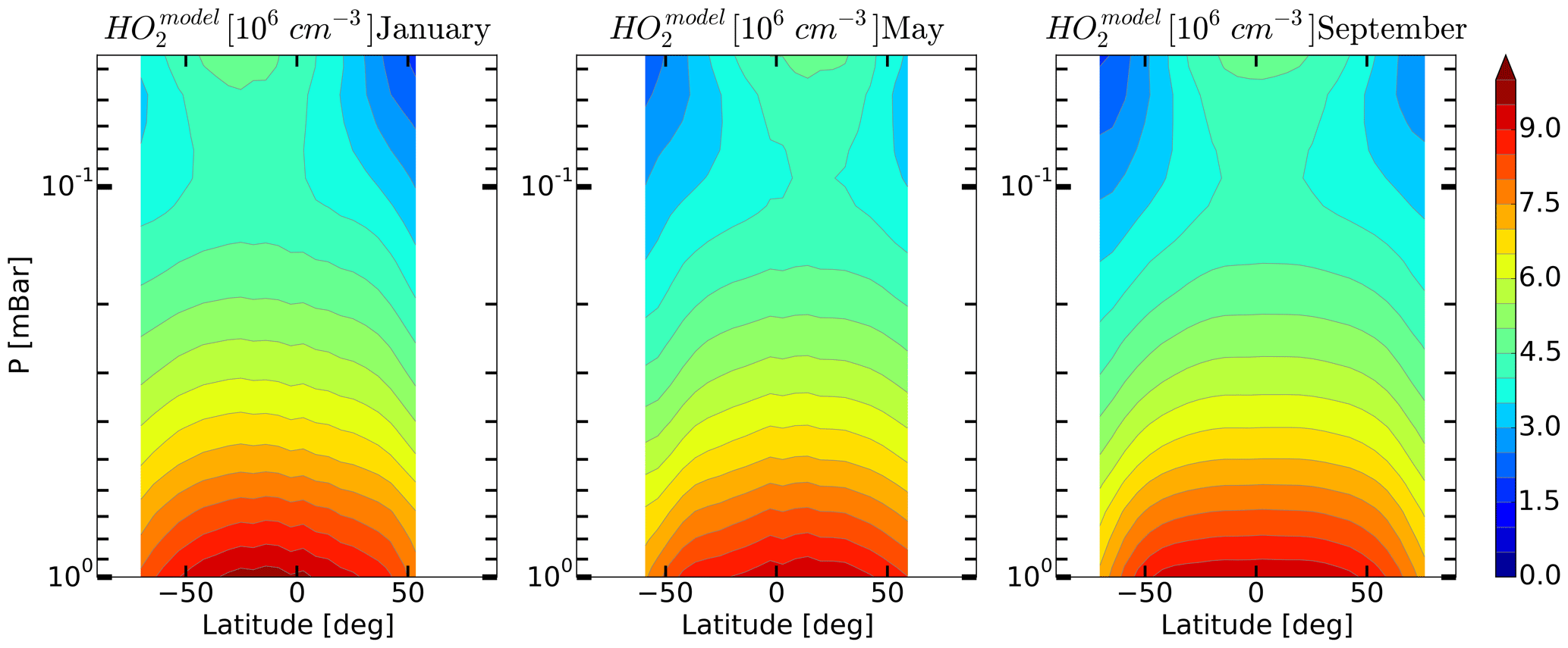
Figure 9 Daytime monthly averaged zonal mean model distributions of HO₂ for January, May, and September.

Figure 10 Daytime mean monthly averaged distributions of HO₂ retrieved by Millán et al. (2015) and relative differences $(<{\mathrm{HO}}_{\mathrm{2}}^{\mathrm{MLS}}>-<{\mathrm{HO}}_{\mathrm{2}\mathrm{offline}}^{\mathrm{MLS}}>)/<{\mathrm{HO}}_{\mathrm{2}\mathrm{offline}}^{\mathrm{MLS}}>$ and $(<{\mathrm{HO}}_{\mathrm{2}}^{\mathrm{ret}}>-<{\mathrm{HO}}_{\mathrm{2}\mathrm{offline}}^{\mathrm{MLS}}>)/<{\mathrm{HO}}_{\mathrm{2}\mathrm{offline}}^{\mathrm{MLS}}>$.

The next important daytime source of OH is specified by reactions (R59) and (R7) involving H₂O, the main source for the HO_x family:

$$\begin{array}{}\text{(R2)}& P_{\mathrm{OH}}^{{\mathrm{H}}_{\mathrm{2}}\mathrm{O}}=\left(k_{\mathrm{59}}+\mathrm{2}\cdot k_{\mathrm{7}}\cdot \mathrm{O}{(}^{\mathrm{1}}\mathrm{D})\right)\cdot {\mathrm{H}}_{\mathrm{2}}\mathrm{O}.\end{array}$$

Figure 3 shows height–latitude cross-sections of $<P_{\mathrm{OH}}^{{\mathrm{H}}_{\mathrm{2}}\mathrm{O}}/P_{\mathrm{OH}}>$ for each month. Comparing Figs. 1 and 3, we conclude that the previously indicated 3–4 % deviation of $<F>$ from 1 in the region between 76 and 86 km is largely due to the neglect of these reactions.

Another source of OH is sporadically activated during charged particle precipitation events and exists for a relatively short time (several days). Solar proton events (SPEs) perturb the ionic composition in the mesosphere and the upper stratosphere considerably and trigger a whole cascade of reactions involving ions, neutral components, and their clusters (e.g., O${}_{\mathrm{2}}^{+}$ ⋅ H₂O). This leads to an additional (to reactions R59 and R7) conversion of H₂O molecules into OH and H (Solomon et al., 1981). The maximum of the OH production rate ($P_{\mathrm{OH}}^{\text{SPE}})$ induced by SPE is located in the polar latitudes in the region of 60–80 km and, as a rule, does not exceed 2×10³ cm⁻³ s⁻¹ (Jackman et al., 2011, 2014). It can be seen from Fig. 2 that at these latitudes and altitudes the $P_{\mathrm{OH}}^{\text{SPE}}/P_{\mathrm{OH}}$ ratio does not exceed 1–2 %, even for the maximum values of $P_{\mathrm{OH}}^{\text{SPE}}$. This means that the impact of $P_{\mathrm{OH}}^{\text{SPE}}$ on Eq. (6) is of the same order of smallness as in the case of reactions (R59) and (R7); hence, it may be neglected. A similar conclusion can be made for other reactions from Table 1, not accounted for by Eq. (6), including the ones involving NO_x in both quiet and perturbed conditions in the mesosphere.

4 Method of statistical evaluation of simultaneous measurement of OH, HO₂, and O₃

The proposed method is based on the statistical Bayesian procedure described in the works by Kulikov et al. (2009b) and Nechaev et al. (2016). It was originally developed for retrieving trace gas concentrations in the mesosphere from ground-based and satellite measurements of other mesospheric components. With respect to the considered evaluation problem, this procedure consists of three steps: (i) constructing a conditional probability density function (PDF) of OH, HO₂, and O₃ concentration values at each altitude z in the selected interval assuming that there is certain measurement data of these components and the algebraic relationship (6) is valid; ii) calculating the first moments of this distribution, i.e., expected value and dispersion of each component using the Metropolis–Hastings algorithm (Chib and Greenberg, 1995) for multidimensional integration; (iii) comparing the obtained results with the initial measurement data.

For constructing posterior PDF it is convenient to introduce vector $\mathit{u}\left\{{\mathrm{HO}}_{\mathrm{2}}^{\mathrm{ret}},{\mathrm{O}}_{\mathrm{3}}^{\mathrm{ret}},{\mathrm{OH}}^{\mathrm{ret}}\right\}$, whose components are the retrieved values of chemical species concentrations at a certain altitude z, and vector $\mathit{x}\left\{{\mathrm{HO}}_{\mathrm{2}}^{\text{m}},{\mathrm{O}}_{\mathrm{3}}^{\text{m}},{\mathrm{OH}}^{\text{m}}\right\}$ composed of experimentally measured values of the components of vector u, $x_j=u_j+{\mathit{\xi }}_j,j=\mathrm{1}.$, where ξ_j is a random error of measuring the jth component of vector u at the altitude z. It is assumed that

1. random variables ξ_j are distributed normally with densities

   $$\begin{array}{}\text{(7)}& w_j\left({\mathit{\xi }}_j\right)={\displaystyle \frac{\mathrm{1}}{{\mathit{\sigma }}_j\sqrt{\mathrm{2}\mathit{\pi }}}}\exp \left(-{\displaystyle \frac{{\mathit{\xi }}_j^{\mathrm{2}}}{\mathrm{2}{\mathit{\sigma }}_j^{\mathrm{2}}}}\right);\end{array}$$

2. ξ_j are mutually independent:

   $$\begin{array}{}\text{(8)}& \mathit{\xi }\left\{{\mathit{\xi }}_{\mathrm{1}},{\mathit{\xi }}_{\mathrm{2}},{\mathit{\xi }}_{\mathrm{3}}\right\}\sim W_{\mathit{\xi }}\left(\mathit{\xi }\right)=\prod _j{w}_j\left({\mathit{\xi }}_j\right),\end{array}$$

   where W_ξ(ξ) is the total PDF of all ξ_j;

3. dispersions σ_j in Eq. (7), that are expected error values, are assumed to be known a priori (in our case they are provided by the MLS retrieval algorithm along with measured data).

   Then the probability to observe vector x is given by the conditional PDF

   $$\begin{array}{}\text{(9)}& P_x\left(\mathit{x}\mathrm{|}\mathit{u}\right)=\int \mathit{\delta }\left(\mathit{x}-\mathit{u}\right)W_{\mathit{\xi }}\left({\mathit{\xi }}^{\mathbf{\prime }}\right){\text{d}}^{\mathrm{3}}{\mathit{\xi }}^{\mathbf{\prime }}=W_{\mathit{\xi }}\left(\mathit{x}-\mathit{u}\right),\end{array}$$

   where δ (...) is the delta function.

The prior relationship of HO${}_{\mathrm{2}}^{\mathrm{ret}}$, O${}_{\mathrm{3}}^{\mathrm{ret}}$, and OH^ret concentrations (Eq. 6) can be written as $u_{\mathrm{3}}=G\left(u_{\mathrm{1}},u_{\mathrm{2}}\right)$. Integrating the left-hand side of Eq. (9) with the conditional PDF of the variable u₃:

$${\displaystyle }{P}_{u_{\mathrm{3}}}\left(u_{\mathrm{3}}\mathrm{|}{u}_{\mathrm{1}},u_{\mathrm{2}}\right)=\mathit{\delta }\left(u_{\mathrm{3}}-G\left(u_{\mathrm{1}},u_{\mathrm{2}}\right)\right),$$

yields a likelihood function of the model

$$\begin{array}{ll}{\displaystyle }{P}_x& {\displaystyle }\left(\mathit{x}\mathrm{|}{u}_{\mathrm{1}},u_{\mathrm{2}}\right)=w_{\mathrm{3}}\left(x_{\mathrm{3}}-G\left(u_{\mathrm{1}},u_{\mathrm{2}}\right)\right)\\ \text{(10)}& {\displaystyle }& {\displaystyle }\cdot w_{\mathrm{1}}\left(x_{\mathrm{1}}-u_{\mathrm{1}}\right)w_{\mathrm{2}}\left(x_{\mathrm{2}}-u_{\mathrm{2}}\right).\end{array}$$

According to Bayes' theorem, the posterior function, i.e., the probability density of latent variables u₁ and u₂, under the condition that x is observed, is defined by the expression

$$\begin{array}{ll}{\displaystyle }& {\displaystyle }P\left(u_{\mathrm{1}},u_{\mathrm{2}}\mathrm{|}\mathit{x}\right)\propto P_x(\mathit{x}\mathrm{|}{u}_{\mathrm{1}},u_{\mathrm{2}})\cdot P_{\text{apr}}\left(u_{\mathrm{1}},u_{\mathrm{2}}\right)\\ {\displaystyle }\propto & {\displaystyle }\exp \left(-{\displaystyle \frac{{\left(x_{\mathrm{1}}-u_{\mathrm{1}}\right)}^{\mathrm{2}}}{\mathrm{2}{\mathit{\sigma }}_{\mathrm{1}}^{\mathrm{2}}}}\right)\cdot \exp \left(-{\displaystyle \frac{{\left(x_{\mathrm{2}}-u_{\mathrm{2}}\right)}^{\mathrm{2}}}{\mathrm{2}{\mathit{\sigma }}_{\mathrm{2}}^{\mathrm{2}}}}\right)\\ \text{(11)}& {\displaystyle }& {\displaystyle }\cdot \exp \left(-{\displaystyle \frac{(x_{\mathrm{3}}-G\left(u_{\mathrm{1}},u_{\mathrm{2}}\right){)}^{\mathrm{2}}}{\mathrm{2}{\mathit{\sigma }}_{\mathrm{3}}^{\mathrm{2}}}}\right)\cdot P_{\text{apr}}\left(u_{\mathrm{1}},u_{\mathrm{2}}\right),\end{array}$$

in which P_apr(u₁,u₂) defines the prior PDF of u₁ and u₂.

The retrieved value of the latent variable $u_{\mathrm{1},\mathrm{2},\mathrm{3}}$ is hereinafter understood as the mean value of the function in Eq. (11):

$$\begin{array}{}\text{(12)}& \begin{array}{l}〈u_{\mathrm{1},\mathrm{2}}〉=\underset{-\mathrm{\infty }}{\overset{\mathrm{\infty }}{\int }}\underset{-\mathrm{\infty }}{\overset{\mathrm{\infty }}{\int }}{u}_{\mathrm{1},\mathrm{2}}\cdot P\left(u_{\mathrm{1}},u_{\mathrm{2}}\mathrm{|}\mathit{x}\right)\mathrm{d}{u}_{\mathrm{1}}\mathrm{d}{u}_{\mathrm{2}},\\ 〈u_{\mathrm{3}}〉=\underset{-\mathrm{\infty }}{\overset{\mathrm{\infty }}{\int }}\underset{-\mathrm{\infty }}{\overset{\mathrm{\infty }}{\int }}G\left(u_{\mathrm{1}},u_{\mathrm{2}}\right)\cdot P\left(u_{\mathrm{1}},u_{\mathrm{2}}\mathrm{|}\mathit{x}\right)\mathrm{d}{u}_{\mathrm{1}}\mathrm{d}{u}_{\mathrm{2}}.\end{array}\end{array}$$

Its dispersion defines the uncertainty in the retrieval:

$$\begin{array}{}\text{(13)}& {\mathit{\sigma }}_{u_j}=\sqrt{〈u_j^{\mathrm{2}}〉-{〈u_j〉}^{\mathrm{2}}},j=\mathrm{1}.,\end{array}$$

where the angle brackets denote averaging in the sense of Eq. (12).

5 MLS/Aura data evaluation and results

We used the latest version (v4.2) of the MLS “standard” product (Livesey et al., 2017) for trace gas concentrations and temperature T within the 1–0.046 mbar pressure interval, where all data are suitable for scientific applications (Wang et al., 2015a, b; Schwartz et al., 2015). We took the daytime data when the solar zenith angle χ<80^∘ for January, May, and September 2005. All data were appropriately screened. “Pressure”, “estimated precision”, “status flag”, “quality”, “convergence”, and “clouds” fields were taken into account. HO₂ data were seen as the day-minus-night difference as prescribed by the MLS data guidelines (Livesey et al., 2017). Following Pickett et al. (2008), each daytime profile of this component measured on a given day at a latitude Lat, a profile resulting from averaging the nighttime profiles of HO₂, measured on the same day in the latitude range of Lat ± 5^∘, was subtracted. This operation eliminates systematic biases affecting HO₂ retrievals, but limits the studied latitude range to the one where MLS observes both daytime and nighttime data.

The integrals in Eqs. (12)–(13) were calculated at every pressure level p for each set of simultaneously measured vertical profiles OH^MLS(p), HO${}_{\mathrm{2}}^{\mathrm{MLS}}\left(p\right)$, O${}_{\mathrm{3}}^{\mathrm{MLS}}\left(p\right)$, T^MLS(p), ${\mathit{\sigma }}_{{\mathrm{OH}}^{\mathrm{MLS}}}\left(p\right)$, ${\mathit{\sigma }}_{{\mathrm{HO}}_{\mathrm{2}}^{\mathrm{MLS}}}\left(p\right)$, and ${\mathit{\sigma }}_{{\mathrm{O}}_{\mathrm{3}}^{\mathrm{MLS}}}\left(p\right)$. The vertical profiles $<{\mathrm{OH}}^{\mathrm{ret}}>\left(p\right)$, $<{\mathrm{HO}}_{\mathrm{2}}^{\mathrm{ret}}>\left(p\right)$, $<{\mathrm{O}}_{\mathrm{3}}^{\mathrm{ret}}>\left(p\right)$, ${\mathit{\sigma }}_{{\mathrm{OH}}^{\mathrm{ret}}}\left(p\right)$, ${\mathit{\sigma }}_{{\mathrm{HO}}_{\mathrm{2}}^{\mathrm{ret}}}\left(p\right)$, and ${\mathit{\sigma }}_{{\mathrm{O}}_{\mathrm{3}}^{\mathrm{ret}}}\left(p\right)$ were found at each point of the globe along the satellite track. Numerical integration was performed by a Monte Carlo method. For each pressure level, a sample of about 5×10⁵ pairs of random variable values $\left\{u_{\mathrm{1}},u_{\mathrm{2}}\right\}=\left\{{\mathrm{HO}}_{\mathrm{2}}^{\mathrm{ret}},{\mathrm{O}}_{\mathrm{3}}^{\mathrm{ret}}\right\}$ distributed with normalized probability density given by Eq. (11) with $P_{\text{apr}}\left(u_{\mathrm{1}},u_{\mathrm{2}}\right)\equiv \mathrm{1}$ was generated with the help of the Metropolis–Hastings algorithm (Chib and Greenberg, 1995). In this case, the statistical moments in Eqs. (12)–(13) were determined by summation over the sample.

A typical example of retrieved profiles HO${}_{\mathrm{2}}^{\mathrm{ret}}$, O${}_{\mathrm{3}}^{\mathrm{ret}}$, and OH^ret (black curves) in comparison with the measured HO${}_{\mathrm{2}}^{\mathrm{MLS}}$, O${}_{\mathrm{3}}^{\mathrm{MLS}}$, and OH^MLS (red curves) is given in Fig. 4. First of all, note that statistics of the retrieved data are in satisfactory agreement with the initial measurement of OH and O₃ concentrations, but not of HO₂. The error of satellite measurement, ${\mathit{\sigma }}_{{\mathrm{HO}}_{\mathrm{2}}^{\mathrm{MLS}}}$, greatly exceeds the uncertainty in the retrieval, ${\mathit{\sigma }}_{{\mathrm{HO}}_{\mathrm{2}}^{\mathrm{ret}}}$, so at some altitudes the values of $<{\mathrm{HO}}_{\mathrm{2}}^{\mathrm{MLS}}>$ (red dashed curves) do not fall within the corresponding intervals $<{\mathrm{HO}}_{\mathrm{2}}^{\mathrm{ret}}>\pm {\mathit{\sigma }}_{{\mathrm{HO}}_{\mathrm{2}}^{\mathrm{ret}}}$. Second, the results of a single measurement of all three components and their retrieved values have considerable uncertainties relative to their means within the whole interval of altitudes. Therefore, the observed and retrieved data should be compared using the commonly accepted approach (e.g., Pickett et al., 2008) of averaging large ensembles of profiles within certain latitude and time ranges, or zones. It is supposed that the noise of satellite measurement instruments is delta-correlated, so that random values corresponding to each single measured or retrieved profile are statistically independent. In this case the dispersion of a measured or retrieved zonal mean profile is determined by summation

$${\displaystyle }{\mathit{\sigma }}_{\mathrm{\Sigma }}^{\mathrm{2}}={\displaystyle \frac{\mathrm{1}}{N^{\mathrm{2}}}}\sum _{k=\mathrm{1}}^N{\mathit{\sigma }}_k^{\mathrm{2}},$$

where N is the number of measured or retrieved profiles within the zone and ${\mathit{\sigma }}_k^{\mathrm{2}}$ is the dispersion of the kth measured or retrieved profile.

The range of latitudes covered by the satellite trajectory was divided into 17 bins 10^∘ each. About 3000 single profiles of each chemical component fall into one bin during a month of MLS/Aura observations. Therefore, the resulting uncertainties due to measurement noise in OH, HO₂, and O₃ concentration profiles (both measured and retrieved) averaged over such ensembles are significantly lower (about one and a half orders of magnitude) than the uncertainties in individual profiles. Examples of such profiles for January, May, and September 2005 are presented in Fig. 5. One can see that the indicated uncertainties are now small enough to make clear conclusions about the extent to which the observed and retrieved profiles agree by comparing their averaged values only, i.e., $<{\mathrm{OH}}^{\mathrm{MLS}}>$, $<{\mathrm{HO}}_{\mathrm{2}}^{\mathrm{MLS}}>$, and $<{\mathrm{O}}_{\mathrm{3}}^{\mathrm{MLS}}>$ and $<{\mathrm{OH}}^{\mathrm{ret}}>$, $<{\mathrm{HO}}_{\mathrm{2}}^{\mathrm{ret}}>$, and $<{\mathrm{O}}_{\mathrm{3}}^{\mathrm{ret}}>$.

Figures 4–6 show monthly averaged zonal mean pressure–latitude cross-sections of $<{\mathrm{HO}}_{\mathrm{2}}^{\mathrm{ret}}>$, $<{\mathrm{HO}}_{\mathrm{2}}^{\mathrm{MLS}}>$, and $\mathrm{\Delta }{\mathrm{HO}}_{\mathrm{2}}=(<{\mathrm{HO}}_{\mathrm{2}}^{\mathrm{ret}}>-<{\mathrm{HO}}_{\mathrm{2}}^{\mathrm{MLS}}>)/<{\mathrm{HO}}_{\mathrm{2}}^{\mathrm{MLS}}>$ as well as similar characteristics for OH and O₃ concentration profiles for three months of the year 2005. First, clearly, the distributions of $<{\mathrm{OH}}^{\mathrm{ret}}>$ and $<{\mathrm{O}}_{\mathrm{3}}^{\mathrm{ret}}>$ are in good qualitative and quantitative agreement with the initial MLS/Aura measurement data at lower altitudes, below ∼ 0.07 and 0.1 mbar, correspondingly. At higher altitudes, the distributions of $<{\mathrm{OH}}^{\mathrm{ret}}>$ reproduce all the main structural features of $<{\mathrm{OH}}^{\mathrm{MLS}}>$, but the retrieved OH concentration has lower values than the observed one with a relative difference ΔOH reaching ∼ 15 % at the top. The distribution of $<{\mathrm{O}}_{\mathrm{3}}^{\mathrm{ret}}>$ above 0.1 mbar, in turn, differs considerably from $<{\mathrm{O}}_{\mathrm{3}}^{\mathrm{MLS}}>$, both in quantity and quality, and ΔO₃ locally reaches 50–60 % and more. Second, for all months there are significant qualitative and quantitative differences between $<{\mathrm{HO}}_{\mathrm{2}}^{\mathrm{ret}}>$ and $<{\mathrm{HO}}_{\mathrm{2}}^{\mathrm{MLS}}>$, the most noticeable one being location of the mesospheric maximum of this component's concentration. According to the observations it is close to 0.1 mbar, while the retrieved data demonstrate the altitudes of about ∼ 0.046 mbar or higher. Our analysis of the applied method of statistical evaluation demonstrates that the higher position of this maximum in the distributions of $<{\mathrm{HO}}_{\mathrm{2}}^{\mathrm{ret}}>$ is influenced by the OH^MLS data in which the mesospheric maximum (see Figs. 6–8) is also located notably higher than 0.1 mbar.

6 Discussion and conclusion

On the basis of the data presented in Sect. 5 we can conclude that, upon the whole, simultaneous OH, HO₂ and O₃ satellite measurements poorly satisfy the photochemical equilibrium condition. This bias is most prominent for the HO₂ component. We can conjecture that a possible explanation for the bias is the significant systematic error in HO₂ measurements, particularly at the height of the mesospheric maximum. This assumption is supported by the calculation of the HO₂ distributions with the use of our 3-D chemical transport model (see Fig. 9). It can be seen that the mesospheric maximum of HO₂ in these months, as well as of the $<{\mathrm{HO}}_{\mathrm{2}}^{\mathrm{ret}}>$ distributions lies above 0.046 mbar.

Moreover, new data on the HO₂ distributions were recently obtained from the MLS measurements. Millán et al. (2015) performed the offline retrieval of daily zonal means of HO₂ profiles using averaged MLS radiances measured in 10^∘ latitude bins. Averaged spectra have a better signal-to-noise ratio, which removes many of the limitations of the MLS standard product for HO₂. In particular, the upper boundary of the altitude region in which daytime data are suitable for scientific use has reached 0.0032 mbar, and the “day-minus-night” correction is not needed at altitudes above 1 mbar. Comparison with various experimental and model data has shown that the offline retrieval reproduces the basic properties of the HO₂ distribution in the mesosphere relatively well (at least qualitatively; Millán et al., 2015).

The offline retrieval product, the alternative data set of daytime HO₂, has recently become publicly available at https://mls.jpl.nasa.gov (last access: 26 May 2018). Figure 10 shows the monthly averaged zonal means of the offline retrieval data ($<{\mathrm{HO}}_{\mathrm{2}\mathrm{offline}}^{\mathrm{MLS}}>)$ and relative differences with retrieved and MLS standard product data $(<{\mathrm{HO}}_{\mathrm{2}}^{\mathrm{MLS}}>-<{\mathrm{HO}}_{\mathrm{2}\mathrm{offline}}^{\mathrm{MLS}}>)/<{\mathrm{HO}}_{\mathrm{2}\mathrm{offline}}^{\mathrm{MLS}}>$ and $(<{\mathrm{HO}}_{\mathrm{2}}^{\mathrm{ret}}>-<{\mathrm{HO}}_{\mathrm{2}\mathrm{offline}}^{\mathrm{MLS}}>)/<{\mathrm{HO}}_{\mathrm{2}\mathrm{offline}}^{\mathrm{MLS}}>$, correspondingly. Figure 10 represents the same time periods as Figs. 6–8. It is worth noting that the distributions $<{\mathrm{HO}}_{\mathrm{2}\mathrm{offline}}^{\mathrm{MLS}}>$ depicted in Fig. 10 represent significantly different amounts of data. The data sets for May and September include 31 and 27 days of measurements, respectively, whereas the January data set encompasses only 4 days. The latter makes the graphs in the first row in Fig. 10 noisier than the others. One can see that the results of the offline HO₂ retrieval show the same features as the results of our evaluation technique in comparison to the standard MLS retrieval, i.e., the height of mesospheric HO₂ maximum is notably higher. We can conclude that the distributions of $<{\mathrm{HO}}_{\mathrm{2}}^{\mathrm{ret}}>$ better match $<{\mathrm{HO}}_{\mathrm{2}\mathrm{offline}}^{\mathrm{MLS}}>$ than $<{\mathrm{HO}}_{\mathrm{2}}^{\mathrm{MLS}}>$, although some quantitative discrepancy between $<{\mathrm{HO}}_{\mathrm{2}}^{\mathrm{ret}}>$ and $<{\mathrm{HO}}_{\mathrm{2}\mathrm{offline}}^{\mathrm{MLS}}>$ also exists. Note that this may be due to systematic errors in the ${\mathrm{HO}}_{\mathrm{2}}^{\mathrm{MLS}}$ distributions, which cannot be excluded within the framework of the introduced technique. For a detailed qualitative and quantitative comparison of $<{\mathrm{HO}}_{\mathrm{2}}^{\mathrm{ret}}>$ and $<{\mathrm{HO}}_{\mathrm{2}\mathrm{offline}}^{\mathrm{MLS}}>$, one should modify the method so that a statistical evaluation of the OH^MLS and O${}_{\mathrm{3}}^{\mathrm{MLS}}$ standard products, and the data of the offline HO₂ retrieval, could be conducted within the framework of a single procedure with no account for the HO${}_{\mathrm{2}}^{\mathrm{MLS}}$ distributions. This modification is under way and will be presented elsewhere.

The proposed method for statistical evaluation of mesospheric species measurements can be readily generalized to other atmospheric photochemical systems that contain short-lived components (see Introduction). It may also be modified for assessing hard-to-measure chemical components, characteristics of atmospheric processes (like wind speed or turbulent diffusion rate), or poorly known reaction rates.