the Creative Commons Attribution 4.0 License.
the Creative Commons Attribution 4.0 License.
 | 25 May 2018
Large-scale tropospheric transport in the Chemistry–Climate Model Initiative (CCMI) simulations
Huang Yang
Darryn W. Waugh
Guang Zeng
Olaf Morgenstern
Douglas E. Kinnison
Jean-Francois Lamarque
Simone Tilmes
David A. Plummer
John F. Scinocca
Beatrice Josse
Virginie Marecal
Patrick Jöckel
Luke D. Oman
Susan E. Strahan
Makoto Deushi
Taichu Y. Tanaka
Kohei Yoshida
Hideharu Akiyoshi
Yousuke Yamashita
Andreas Stenke
Laura Revell
Timofei Sukhodolov
Eugene Rozanov
Giovanni Pitari
Daniele Visioni
Kane A. Stone
Robyn Schofield
Antara Banerjee
Understanding and modeling the large-scale transport of trace gases and aerosols is important for interpreting past (and projecting future) changes in atmospheric composition. Here we show that there are large differences in the global-scale atmospheric transport properties among the models participating in the IGAC SPARC Chemistry–Climate Model Initiative (CCMI). Specifically, we find up to 40 % differences in the transport timescales connecting the Northern Hemisphere (NH) midlatitude surface to the Arctic and to Southern Hemisphere high latitudes, where the mean age ranges between 1.7 and 2.6 years. We show that these differences are related to large differences in vertical transport among the simulations, in particular to differences in parameterized convection over the oceans. While stronger convection over NH midlatitudes is associated with slower transport to the Arctic, stronger convection in the tropics and subtropics is associated with faster interhemispheric transport. We also show that the differences among simulations constrained with fields derived from the same reanalysis products are as large as (and in some cases larger than) the differences among free-running simulations, most likely due to larger differences in parameterized convection. Our results indicate that care must be taken when using simulations constrained with analyzed winds to interpret the influence of meteorology on tropospheric composition.
- Article
(4891 KB) - Full-text XML
-
Supplement
(837 KB) - BibTeX
- EndNote


The distributions of greenhouse gases (GHGs) and ozone-depleting substances (ODSs) are strongly influenced by large-scale atmospheric transport. In the extratropics the midlatitude jet stream influences the long-range transport of pollutants and water vapor into the Arctic (e.g., Eckhardt et al., 2003; Shindell et al., 2008; Liu and Barnes, 2015) and surface ozone variability over the western United States (Lin et al., 2015). In the tropics, low-level inflow and seasonal variations in the Hadley cell modulate trace gas variability in the tropics and interhemispheric transport into the Southern Hemisphere (SH) (Prather et al., 1987; Mahlman, 1997; Holzer, 1999; Bowman and Erukhimova, 2004).
There are large uncertainties in our understanding of how large-scale atmospheric transport influences tropospheric composition. This is largely because transport is difficult to constrain directly from observations and because global-scale tropospheric transport properties differ widely among models. For example, Denning et al. (1999) found more than a factor of 2 difference in the interhemispheric exchange rate among simulations produced using both offline chemical transport models (CTMs) and online free-running general circulation models (GCMs).
One approach to reducing this uncertainty has been to use models constrained with analysis fields, although comparisons of the transport properties among these simulations also reveal large differences. For example, Patra et al. (2011) showed that the interhemispheric transport differences among the CTMs participating in the TransCOM experiment differ by up to a factor of 2, with models featuring faster interhemispheric transport also exhibiting a faster exchange of methane and methyl chloroform. It is not clear, however, whether these differences reflect subgrid-scale differences among CTMs or differences in the prescribed large-scale flow, since that study included simulations that were constrained with three different sources of meteorological fields.
More recently, Orbe et al. (2017) compared the global-scale tropospheric transport properties among free-running simulations using internally generated meteorological fields and simulations constrained with analysis fields using models developed at the NASA Goddard Space Flight Center and the Community Earth System Model framework (CESM; run at the National Center for Atmospheric Research, NCAR). They showed that the large-scale transport differences among simulations constrained with analysis fields are as large as (and in some cases larger than) the differences among free-running simulations. Furthermore, they found that these differences – manifest over southern high latitudes as a 0.6-year (or ∼ 30 %) difference in the mean age since air was last at the Northern Hemisphere (NH) midlatitude surface – were associated with large differences in (parameterized) convection, particularly over the NH tropics and subtropics. By comparison, the mean age differences between the free-running simulations were found to be negligible, which is consistent with much more similar convective mass fluxes.
The results in Orbe et al. (2017) indicate that care must be taken when using simulations constrained with analysis fields to interpret the influence of meteorology on tropospheric composition. It is not clear, however, if the conclusions from that study reflect only that particular subset of models and/or the particular ways in which those models were constrained with analysis fields. To this end we exploit the broad range of both free-running online and offline (i.e., nudged and CTM) simulations submitted to the recent IGAC/SPARC Chemistry–Climate Model Initiative (CCMI) (Eyring et al., 2013) in order to test some of the key findings in that study. In particular, we focus on the CCMI hindcast simulations of the recent past, which include simulations constrained with both prescribed and internally generated meteorological fields, while sea surface temperatures (SSTs) and sea ice concentrations (SICs) are taken from observations. Thus, the CCMI hindcast experiment provides a relatively clean framework for assessing the influence of different meteorological fields on large-scale atmospheric transport.
As in Orbe et al. (2017) we focus on large-scale tropospheric transport diagnosed from idealized tracers that, unlike the usual basic flow diagnostics (e.g., mean winds, stream functions, mean eddy diffusivities), represent the integrated effects of advection and diffusion while cleanly disentangling the roles of transport from chemistry and emissions. Furthermore, unlike previous intercomparisons that have diagnosed atmospheric transport in terms of one single timescale (e.g., the interhemispheric exchange rate; Denning et al., 1999; Patra et al., 2011), we utilize tracers with different prescribed atmospheric lifetimes and different source regions in order to probe the broad range of timescales and pathways over which tropospheric transport occurs (Orbe et al., 2016). Following a brief exposition of the methodology in Sect. 2 we present results in Sect. 3 and conclusions in Sect. 4.
2.1 Models and experiments
Our analysis uses the models participating in CCMI, which builds upon previous chemistry–climate model intercomparisons, including the SPARC Report on the Evaluation of Chemistry–Climate Models (SPARC CCMVal, 2010) and the Atmospheric Chemistry and Climate Model Intercomparison Project (ACCMIP) (Lamarque et al., 2013), by including several coupled atmosphere–ocean models with a fully resolved stratosphere. For example, more (nine) models are atmosphere–ocean (versus only one in CCMVal-2 and one in ACCMIP) and more models incorporate novel (e.g., cubed-sphere) grids (Morgenstern et al., 2017).
We focus only on those CCMI model simulations that output the idealized tracers (Tables 1 and 2). We present results from the pair of hindcast REF-C1 (simply C1) and REF-C1SD (or C1SD) simulations, which were constrained with observed SSTs and SICs. For each model, we analyze the first ensemble member “r1i1p1” from the REF-C1 and REF-C1SD simulations. Whereas the REF-C1 experiment simulates the recent past (1960–2010) using internally generated meteorological fields, the REF-C1SD or C1 “specified dynamics” simulation is constrained with (re)analysis meteorological fields and correspondingly only spans the years 1980–2010. Note that both online nudged simulations and offline CTMs are used, as indicated in the simulation name. Furthermore, while we have also examined tracer output from the REF-C2 simulation, which used SSTs from a coupled atmosphere–ocean model simulation, we find that the differences in the idealized tracers between the REF-C2 and REF-C1 simulations are significantly smaller than among the hindcast (C1 versus C1SD) simulations. For that reason, from here on we exclude the REF-C2 results from our discussions.
Strahan et al. (2013)Table 1Details of the model integrations in which columns 3–6 correspond to the horizontal resolution, the number of vertical levels and model top, the source of meteorological fields and reference for the model's convective parameterizations. T21 and T42 correspond to quadratic grids of approximately ∼ 5.6∘ × 5.6∘ and ∼ 2.8∘ × 2.8∘, respectively. Two types of model experiments are examined: the REF-C1SD and REF-C1 simulations. Both REF-C1 and REF-C1SD are constrained with observed sea surface temperatures (SSTs) and sea ice concentrations (SICs). Whereas the REF-C1 experiment uses internally generated (or free-running) meteorological fields, the C1SD or C1 “specified dynamics” simulation is constrained with (re)analysis meteorological fields. Note that both CTMs and nudged simulations are included in the REF-C1SD suite of model simulations (see column 6). In cases in which individual modeling agencies performed multiple C1SD simulations (e.g., NASA and NCAR) we append a “V1/V2” to the simulation name.
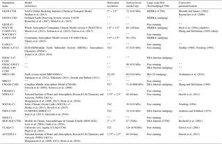
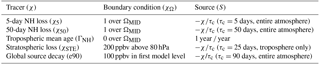
Table 2Table of idealized tracers, χ, integrated in the simulations. All tracers (χ) satisfy the tracer continuity equation, , in the interior of the atmosphere (that is, outside of Ω), where 𝒯 is the linear advection–diffusion transport operator and S denotes interior sources and sinks. For the first three tracers (rows 2–4) Ω is taken to be the NH midlatitude surface, ΩMID, which is defined throughout as the first model level spanning latitudes between 30 and 50∘ N. The last two tracers, referred to throughout as the global source tracers, include the stratospheric tracer χSTE, which is set to 200 ppbv for pressures less than or equal to 80 hPa and decays uniformly in the troposphere at a loss rate τd=25 days−1 (row 5). The e90 tracer is uniformly emitted over the entire surface layer and decays exponentially at a rate of 90 days−1 such that concentrations greater than 125 ppb tend to reside in the lower troposphere and concentrations less than 50 ppb reside in the stratosphere (row 6).
The simulations presented in Orbe et al. (2017) using models from NASA and NCAR are included in our analysis and denoted in all figures using a color convention that is similar to what was used in that study. Note that this subset of runs includes two REF-C1SD simulations per modeling group. In particular, the GEOS-CTM and GEOS-C1SD simulations refer to one simulation of the NASA Global Modeling Initiative (GMI) Chemical Transport Model (Strahan et al., 2013) and one simulation of the Goddard Earth Observing System General Circulation Model version 5 (GEOS-5) (Reinecker et al., 2007; Molod et al., 2015); they are both constrained with fields taken from the Modern-Era Retrospective Analysis for Research and Applications (MERRA) (Rienecker et al., 2011). Meanwhile, the WACCM-C1SDV1 and WACCM-C1SDV2 correspond to two simulations of the Whole Atmosphere Community Climate Model (Marsh et al., 2013) nudged to MERRA meteorological fields using two different relaxation timescales (i.e., 50 and 5 h).
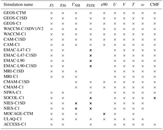
Table 3List of the model simulations for which the idealized tracers (χ5, χ50, ΓNH, χSTE and e90) and dynamical fields (U, V, ω, T and parameterized convective mass fluxes – CMFs) were available. Thin crosses denote fields that output in simulations. Thick crosses denote fields that were output, but were not correctly implemented.
In addition to differences among the REF-C1 and REF-C1SD experiments, the models differ widely in terms of their horizontal resolution, which ranges from ∼ 6∘ (e.g., ULAQ) to ∼ 2∘ (e.g., NCAR and NASA), vertical resolution and choices of subgrid-scale (i.e., turbulence and convective) parameterizations (Morgenstern et al., 2017). Table 1 summarizes some of the main differences among the models and the method by which the large-scale flow was constrained in the REF-C1SD simulations (i.e., CTM versus nudging). For more details please refer to the comprehensive overview presented in Morgenstern et al. (2017).
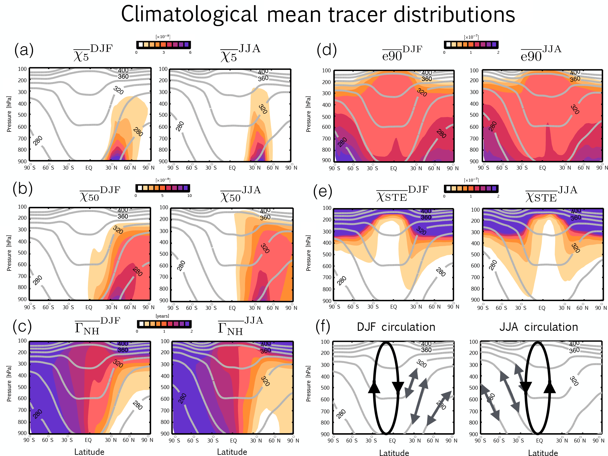
Figure 1Climatological mean December–January–February (DJF) (a–c) and June–July–August (JJA) (d–f) zonally averaged distributions of the 5-day idealized loss tracer χ5 (a), the 50-day idealized loss tracer χ50 (b), the mean age since air was last at the NH midlatitude surface ΓNH (c), the stratospheric global source tracer χSTE (d) and the global surface source tracer e90 (e). Schematic representations of the seasonally averaged mean meridional circulation, overlaid with arrows denoting eddy mixing, are shown in panel (f). 2000–2009 climatological means are shown for the NASA Global Modeling Initiative (GMI) Chemical Transport Model (CTM), which is constrained with MERRA meteorological fields and denoted in all remaining figures as the GEOS-CTM simulation. Climatological seasonal mean dry potential temperature is shown in the grey contours.
Finally, we complement our analysis of the idealized tracers with comparisons of the models' convective mass fluxes, horizontal and vertical winds, and temperature fields (when available; Table 3). All tracer and dynamical variables were available as monthly mean output on native model levels. Therefore, we interpolated all output to a standard pressure vector with 4 pressure levels in the stratosphere (10, 30, 50 and 80 hPa) and 19 pressure levels in the troposphere spaced every 50 hPa between 100 and 1000 hPa. Note that values for pressure levels below the surface topography are treated as missing (NaN) values for all simulations. To construct all of the multi-model means (denoted in the figures using solid grey lines) we first interpolated all model output to the same 1∘ latitude by 1∘ longitude grid and then took the average among the models. As in Orbe et al. (2017) our focus is on seasonal averages over December–January–February (DJF) and June–July–August (JJA) and on 10-year climatological means over the time period 2000–2009, which are denoted throughout using overbars.
2.2 Idealized tracers
Several of the idealized tracers examined in this study (Table 2) were discussed in Orbe et al. (2016, 2017). Figure 1 shows boreal winter (DJF) and boreal summer (JJA) climatological mean distributions of the tracers for one model simulation, which has been chosen purely for illustrative purposes. This is the GEOS-CTM simulation that was presented in Orbe et al. (2017) and described in the previous section. Schematic representations of the seasonally averaged mean meridional circulation in the tropics and arrows denoting mixing by eddies over midlatitudes are also shown to help guide the interpretation of the tracer distributions (Fig. 1f).
Three of the tracers' boundary conditions are zonally uniform and are defined over the same NH surface region over midlatitudes, ΩMID, which we define as the first model level spanning all grid points between 30 and 50∘ N (rows 2–4 in Table 2, Fig. 1a–b). The first two tracers, χ5 and χ50, referred to throughout as the 5-day and 50-day idealized loss tracers, are fixed to a value of 100 ppb over ΩMID and undergo spatially uniform exponential loss at rates of 5 and 50 days−1, respectively. The climatological mean distributions of the loss tracers, denoted throughout as and , decrease poleward away from the midlatitude source region during boreal winter when tracer isopleths coincide approximately with isentropes that intersect the Earth's surface, reflecting the strong influence of isentropic mixing on surface source tracer distributions over middle and high latitudes (Fig. 1f). Note, however, that this is merely an approximation, since vertical mixing by synoptic eddies and moist convection renders the tracer isolines steeper than dry isentropic surfaces. During summer, the idealized loss tracer patterns extend significantly higher into the upper troposphere over midlatitudes, which is consistent both with weaker isentropic transport over the northern extratropics and stronger convection over the continents (Klonecki et al., 2003; Stohl, 2006; Orbe et al., 2015). Compared to , which is mainly confined to the NH extratropics, large values of span the NH subtropics and tropics.
The third NH midlatitude tracer, ΓNH, is initially set to a value of zero throughout the troposphere and held to zero thereafter over ΩMID (Fig. 1c). Elsewhere over the rest of the model surface layer and throughout the atmosphere, ΓNH is subject to a constant aging of 1 year ∕ year so that its statistically stationary value, the mean age, is equal to the average time since the air at a given location in the troposphere last contacted the NH midlatitude surface ΩMID (Waugh et al., 2013). The strongest meridional gradients in the mean age ΓNH, which increases from ∼ 3 months in the NH extratropical lower troposphere to ∼ 2 years over SH high latitudes, are located in the tropics and migrate north and south in concert with seasonal shifts in the Intertropical Convergence Zone (ITCZ) and the mean meridional circulation (Fig. 1f) (Waugh et al., 2013).
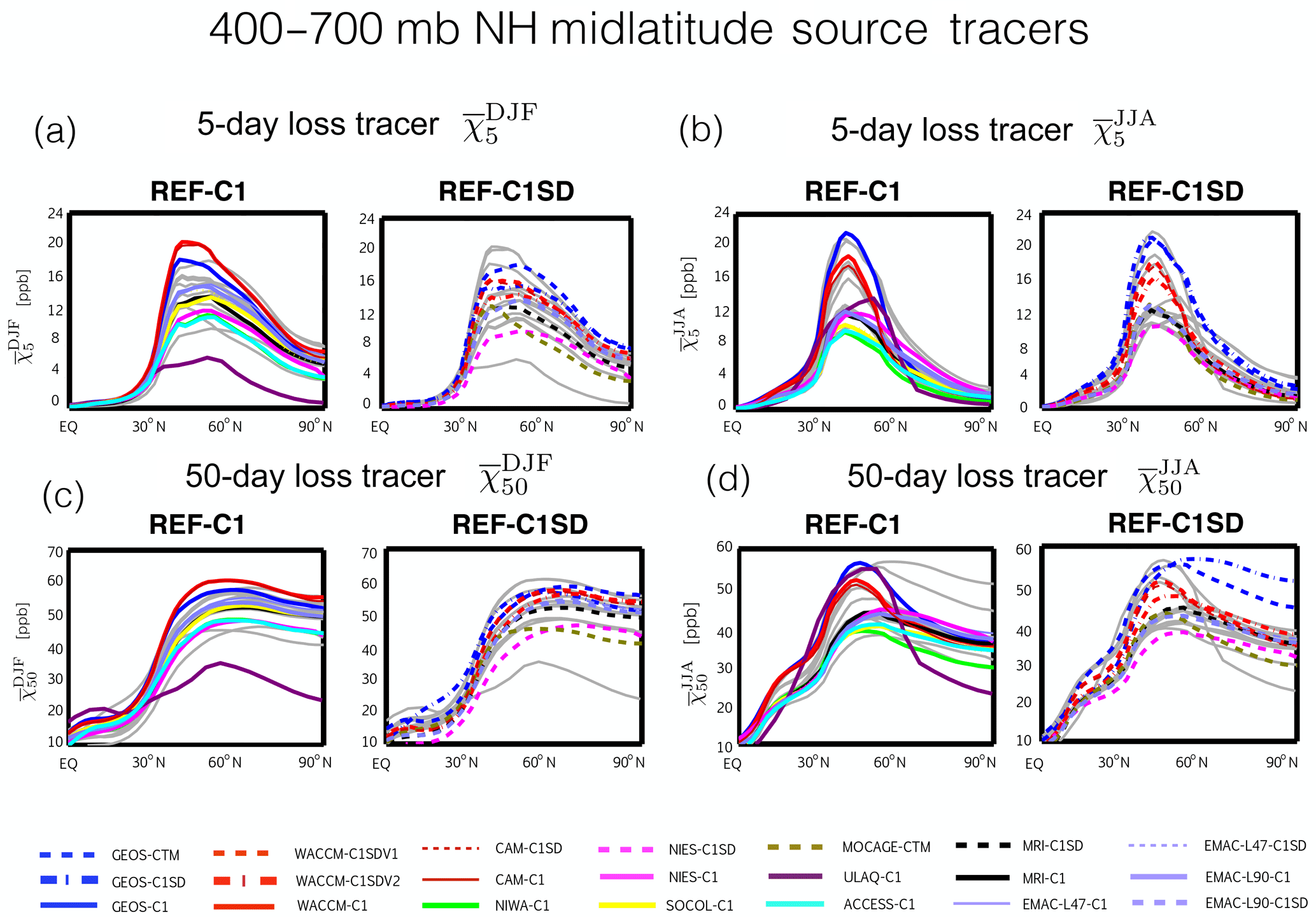
Figure 2Meridional profiles of the 400–700 hPa zonally averaged DJF (a, c) and JJA (b, d) 5-day and 50-day loss tracers, and . Dashed lines in panels (b, d) correspond to the REF-C1SD simulations, which are constrained with analysis meteorological fields, while solid lines in panels (a, c) correspond to the free-running REF-C1 simulations. Grey solid lines in each panel correspond to the REF-C1SD and REF-C1 simulations in panels (a, c) and (b, d), respectively. Note that the x axis only spans the Northern Hemisphere.
In addition to the NH midlatitude source tracers, we also examine two other tracers with global sources. The first tracer, χSTE, is set to a constant value of 200 ppb above 80 hPa and undergoes spatially uniform exponential loss at a rate of 25 days−1 in the troposphere. The second tracer, e90, is uniformly emitted over the surface layer and decays exponentially at a rate of 90 days−1 such that mixing ratios greater than 125 ppb tend to reside in the lower troposphere and mixing ratios smaller than 50 ppb reside in the stratosphere (Prather et al., 2011). While their mean gradients are opposite in sign, due to differences in their boundary conditions, both tracers feature pronounced signatures of isentropic transport in the subtropical upper troposphere along isentropes spanning the middleworld (Hoskins, 1991). This is evident in the plume of large mixing ratios of χSTE and, conversely, small concentrations of e90 that extends down from the tropopause to the subtropical surface (Fig. 1d–e). The seasonality of this isentropic transport is captured by the relatively larger (smaller) values of χSTE (e90) in the northern subtropical upper troposphere during winter compared to during summer (and vice versa in the SH).
3.1 Transport to Northern Hemisphere high latitudes
3.1.1 Differences in transport
Meridional profiles of and , averaged over the middle troposphere (400–700 hPa), differ widely among the simulations over the NH extratropics (Fig. 2). Over northern midlatitudes differs by up to a factor of 5 during boreal winter and a factor of 2–3 during boreal summer. The spread in the 50-day loss tracer, , is similar, which is consistent with the strong compact relationship between the loss tracers such that simulations featuring low concentrations of also feature low concentrations of (and vice versa; see also Fig. 4a below). During summer, the differences in extend all the way to the pole, where ranges between ∼ 20 and 50 ppb among the simulations. Note that these differences are overall much larger than the differences among the simulations presented in Orbe et al. (2017) (red and blue lines, Fig. 2), which feature consistently larger concentrations of and over northern middle and high latitudes compared to the other simulations, indicative of more efficient poleward transport in those models.
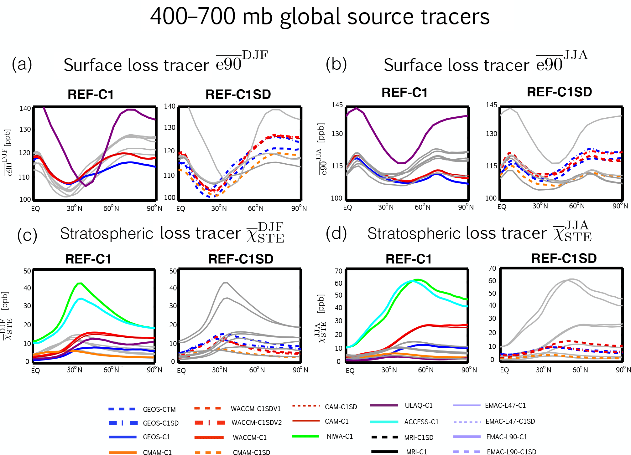
Figure 3Same as Fig. 2, except for the stratospheric and surface global source tracers, e90 (a, b) and χSTE (c, d).
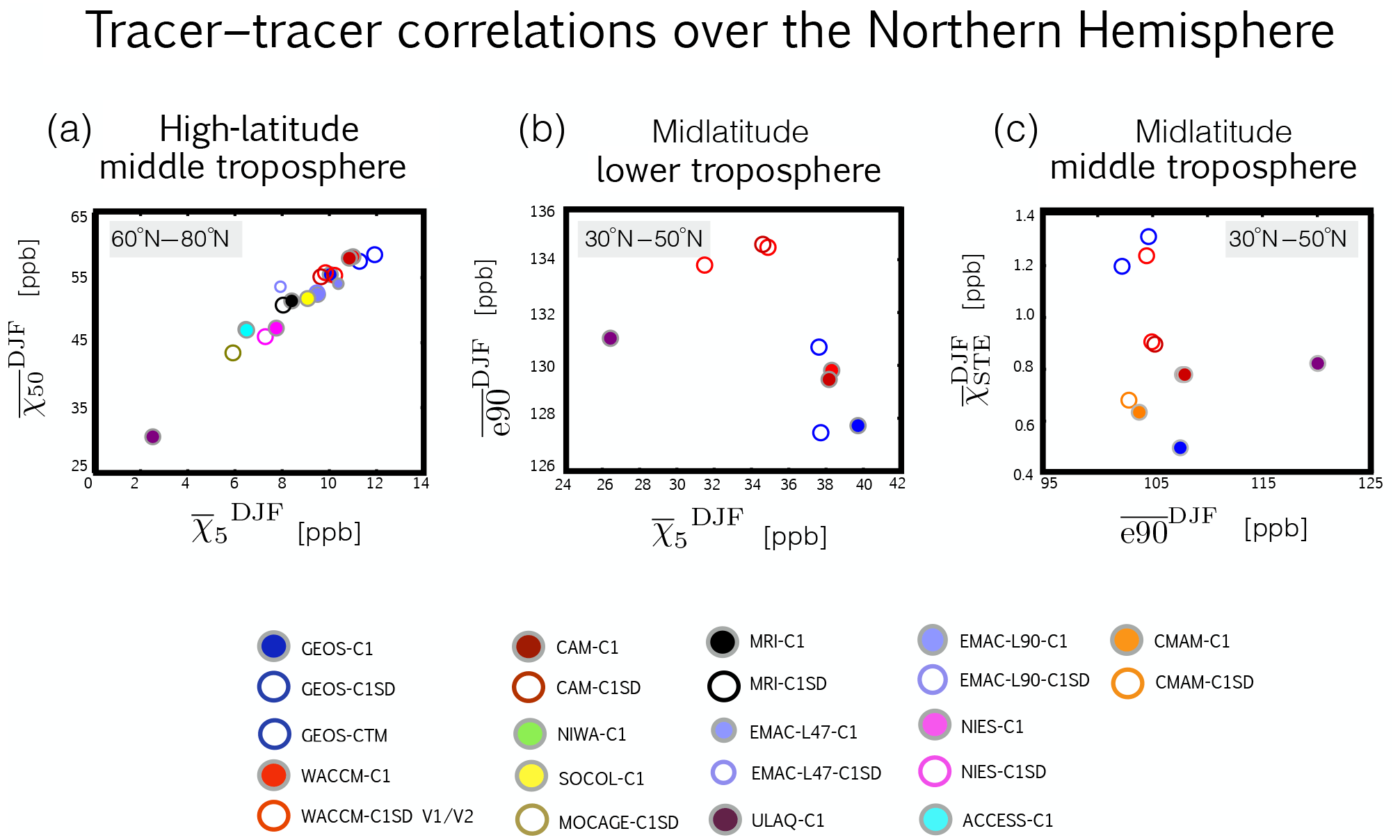
Figure 4(a) Correlations of 400–700 hPa averages of and averaged over latitudes spanning 60 and 80∘ N. (b) Correlations of and averaged over 700–900 hPa and over the midlatitude source region. (c) Same as panel (b), except for and over 400–700 hPa. The different colors correspond to the different simulations, with open circles denoting REF-C1SD simulations and closed circles corresponding to REF-C1 (grey outline). Circles denote the climatological boreal winter mean over 2000–2009.
Interestingly, the differences in the concentrations of and among the C1SD simulations are as large as the differences among the C1 simulations. For example, the 5-day loss tracer concentrations over midlatitudes range between 9 and 22 ppb during boreal summer among both the C1 and C1SD simulations (Fig. 2b). During boreal winter the spread among the C1 simulations is slightly larger, but closer inspection shows that this only reflects the inclusion of one outlier simulation (Fig. 2a, c). Overall, this is consistent with Orbe et al. (2017), who found that the transport differences between two simulations of GEOS-5 and WACCM constrained with fields taken from MERRA were as large as (and at places larger than) the differences between free-running simulations generated using the same models.
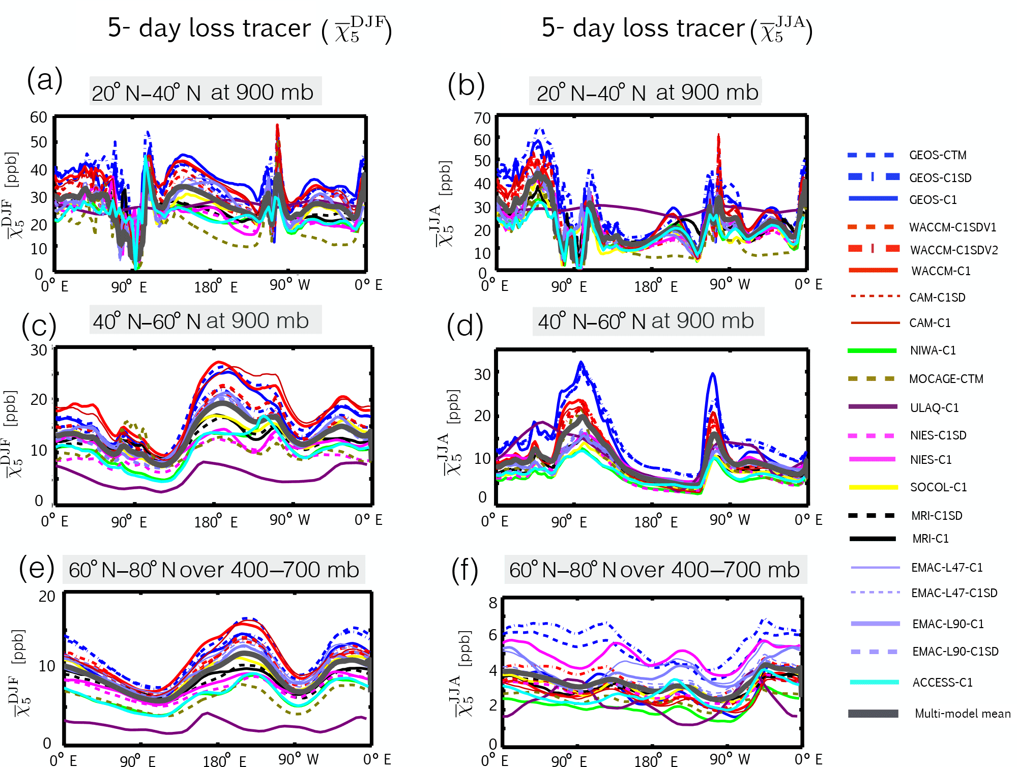
Figure 5Zonal profiles of the climatological mean 5-day idealized loss tracer averaged over 900 hPa and over latitudes spanning 20–40∘ N (a, b) and 40–60∘ N (c, d) and over 400–700 hPa over latitudes between 60 and 80∘ N (e, f). Profiles are shown for DJF (a, c, e) and JJA (b, d, f). Dashed lines correspond to the REF-C1SD simulations, which are constrained with analysis meteorological fields, while solid lines correspond to the free-running REF-C1 simulations. The thick dark grey line represents the multi-model mean.
Comparisons of the global source tracer e90 also reveal large differences among the simulations (Fig. 3). The spread in e90 mixing ratios is similar in magnitude to the spread in the concentrations of the idealized loss tracers, which is consistent with the fact that they all have prescribed surface mixing ratios. At the same time, the relationship between e90 and the midlatitude-sourced tracers is complicated and depends sensitively on latitude. In particular, over the southern edge of the NH midlatitude source region we find that e90 and χ5 are positively correlated such that simulations with relatively large mixing ratios of χ5 and χ50 (blue and red lines in Fig. 2a, c) also feature relatively larger mixing ratios of e90 (Fig. 3a). Over the middle and northern edge of the midlatitude source region, however, the tracers exhibit an inverse (and relatively compact) relationship (Fig. 4b). While this inverse relationship is not intuitive, it is consistent with differences in the meridional gradients of the tracers, wherein χ5 (e90) increases (decreases) moving poleward from the northern subtropics over northern midlatitudes. Perhaps fortuitously, the NH midlatitude tracers are only sourced in the region of strongest isentropic mixing so that χ5 always decreases along an isentropic surface as ones moves from the midlatitude surface poleward to the Arctic (Fig. 1a). By comparison, e90 features its largest concentrations over the Arctic (Fig. 1d) so that stronger mixing over midlatitudes can actually dilute tracer mixing ratios along a given isentrope. Thus, the relationship between the surface-sourced tracers is not straightforward, but rather sensitive to how two-way mixing operates on different (and at places opposite) along-isentropic tracer gradients. More work is needed to disentangle this relationship but is beyond the scope of the current study.
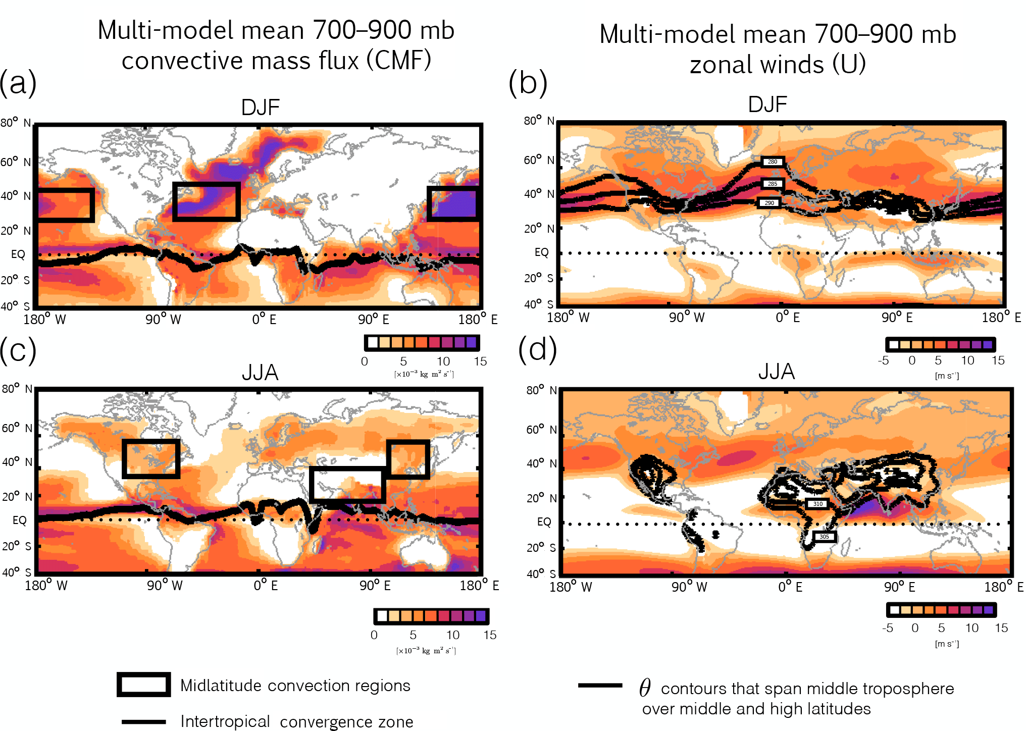
Figure 6Maps of the 700–900 hPa averaged multi-model mean convective mass flux (a, c) and zonal winds (b, d) for DJF (a, b) and JJA (c, d). The multi-model seasonal mean Intertropical Convergence Zone, calculated as the latitude of maximum surface convergence, is shown in the thick black lines in panels (a, c). Black boxes denote the midlatitude convection regions over which the scatterplots in Fig. 8 are evaluated. The thick dark lines in panels (b, d) correspond to the regions where the potential temperature surfaces that span the middle- and high-latitude upper troposphere intersect the NH midlatitude surface, as shown in Fig. 1.
The spread in χSTE among the CCMI simulations is also large (Fig. 3c–d). However, care must be taken when interpreting differences in χSTE as solely reflecting differences in stratosphere–troposphere exchange. In particular, the distribution of χSTE in the outlier simulations (i.e., NIWA C1 and ACCESS C1) may reflect the fact that these models use a hybrid-height vertical coordinate such that the tracer's 80 hPa upper boundary condition is not parallel to any model level and therefore more easily communicated to lower levels (Supplement Fig. S1). Furthermore, while the NIWA and ACCESS simulations use essentially the same model, we note that there are small differences between them that may reflect differences in computing platforms.
Among the other simulations, by comparison, the differences in χSTE emerge below the tropopause, where they more likely reflect differences in isentropic mixing in the subtropical upper troposphere. Among those simulations there is a relatively compact relationship between and during boreal winter over the northern subtropical upper troposphere (Fig. 4c), which is consistent with the Abalos et al. (2017) analysis of a free-running integration of WACCM similar to the WACCM-C1 simulation presented in this study, albeit constrained with model-generated sea surface temperatures and sea ice concentrations. Similar to the findings in that study, our results suggest that both tracers may be useful metrics for discerning stratosphere–troposphere exchange differences among models. Finally, comparisons of the spatial distributions of χSTE fail to reveal any consistencies with differences in tropopause height among the simulations, which are not negligible (Supplement Fig. S2). This indicates that differences in tropopause height are not likely to be the primary drivers of the χSTE differences within the CCMI ensemble. Furthermore, we note that special care must be taken when examining the χSTE tracer output since some modeling groups applied exponential loss at all levels below 80 hPa (instead of the tropopause, as recommended).
Zonal profiles of reveal that differences in the loss tracer distributions over the Arctic reflect differences in isentropic transport originating over the northern subtropical oceans (Fig. 5). During winter large differences in emerge over the oceans in the lower troposphere (900 mb; Fig. 5c) and propagate along isentropes towards high latitudes downstream of the storm tracks (180∘ E–120∘ W, 60∘ W–20∘ E; Fig. 5e). By comparison, during boreal summer, the large differences in that emerge in the subtropics over land (120–60∘ W, 30–120∘ E; Fig. 5b) remain relatively confined over midlatitudes. Rather, the differences in over the Arctic more likely reflect differences that emerge over the midlatitude oceans over the northern edge of the source region (Fig. 5d). We interpret these transport differences next in terms of differences in the large-scale flow and (parameterized) convection among the simulations.
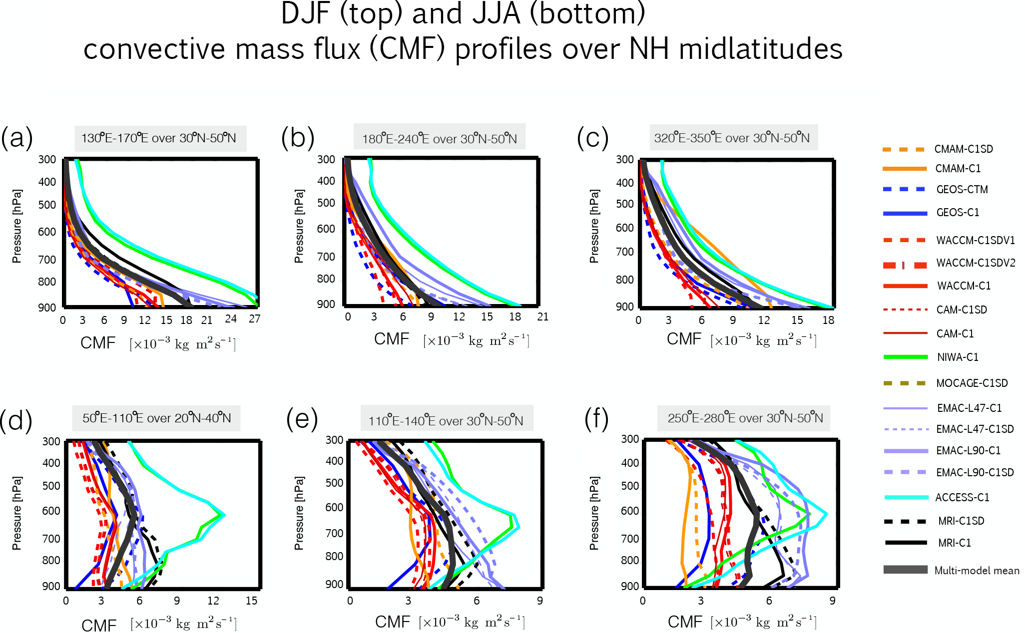
Figure 7Vertical profiles of the convective mass flux evaluated over regions of strong midlatitude convection (black boxes in Fig. 6) during DJF (a–c) and JJA (d–f). The thick dark grey line represents the multi-model mean and dashed lines correspond to the REF-C1SD simulations, while solid lines correspond to the free-running REF-C1 simulations.
3.1.2 Differences in northern midlatitude convection and large-scale flow
One approach to interpreting the large differences in poleward transport among the CCMI simulations is to compare the (parameterized) convection and horizontal flow fields over northern midlatitudes (Fig. 6). During winter the multi-model mean convective mass fluxes () in the lower troposphere (700–900 mb; Fig. 6a) are concentrated over the Pacific and western Atlantic (black boxes). These regions coincide with the climatological mean position of warm conveyer belts at the midlatitude jet entrance regions (Eckhardt et al., 2004) and with low values of potential temperature (280 K < θ < 290 K) approximately along which surface mixing ratios of propagate poleward into the upper and middle high-latitude troposphere (Figs. 1a and 6b).
By comparison, during boreal summer the (parameterized) convective mass fluxes are generally weaker over midlatitudes and shift from the oceans toward land, coincident with weaker and zonally shifted storm tracks. Seasonal changes in the thermal structure of the extratropics also indicate that the Arctic is isentropically isolated from the northern midlatitude surface during summer compared to winter (Klonecki et al., 2003). The CCMI simulations capture this seasonality well in terms of both the convective mass flux distributions (Fig. 6c) and in the redistribution of potential temperature surfaces (Fig. 6d). Any differences in transport among the simulations that emerge over the northern midlatitude surface are therefore more likely to be confined to the midlatitude upper troposphere during boreal summer compared to during winter.
Comparisons of the vertical profiles of the convective mass fluxes (CMFs) over northern midlatitudes (black boxed regions in Fig. 6) reveal large differences in (parameterized) convection among the models during both boreal winter and summer (Fig. 7). Among the “weak midlatitude convection” simulations (i.e., NASA and NCAR), the strength of is at places half (western Pacific) and one-third (western Atlantic) the strength in the “strong midlatitude convection” simulations (i.e., NIWA, ACCESS and EMAC). Note that the latter simulations use convection parameterizations that have a diagnostic closure scheme based on large-scale convergence (i.e., based on that of Tiedtke, 1989), whereas the former simulations utilize relaxed and/or triggered adjustment schemes in which adjustments to explicitly defined moist-convective equilibrium states are partly relaxed (Arakawa, 2004) (Table 1). While the former class of parameterizations tends to produce excessive precipitation relative to observations (Forster et al., 2007), further analysis of the differences among the models' convection schemes is beyond the scope of this study.
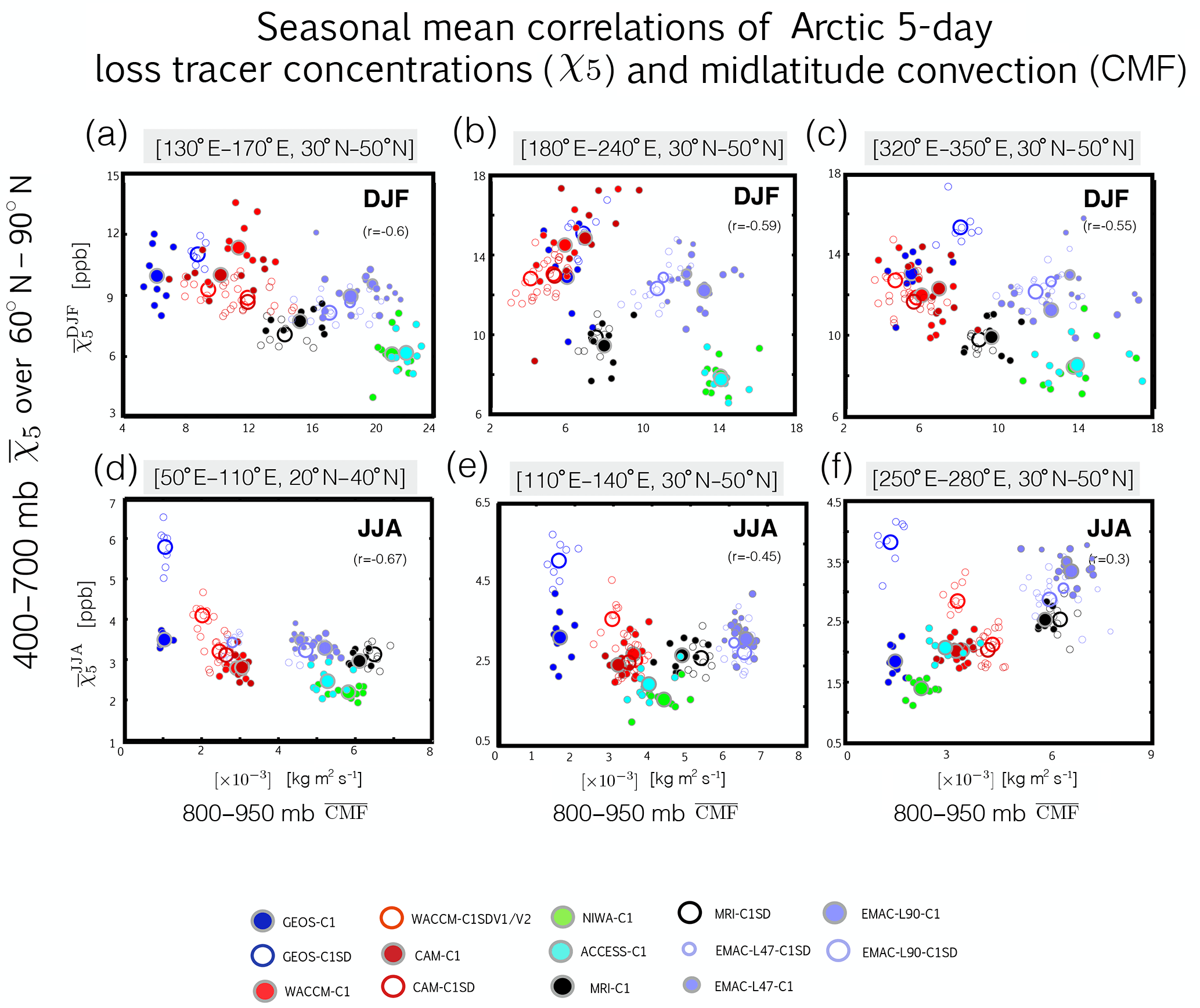
Figure 8Scatterplots showing negative correlations between the strength of parameterized convection in the midlatitude lower troposphere, represented by the 800–950 hPa averaged convective mass flux (), and mid-tropospheric (400–700 hPa) concentrations of the 5-day idealized loss tracer averaged poleward of 60∘ N. The convection regions coincide with the black boxed regions shown in Fig. 6. The different colors correspond to the different simulations, with open circles denoting REF-C1SD simulations and closed circles corresponding to REF-C1 (grey outline) simulations. Small circles correspond to individual years within the 2000–2009 climatological mean period, while large circles denote the climatological mean.
Closer inspection of the loss tracer profiles at 30∘ N during boreal winter reveals that simulations with strong convection over the oceans also feature steeper vertical profiles of compared to models with weaker convection (not shown). This reflects the influence of convective updrafts mixing large near-surface concentrations aloft and convective downdrafts mixing low upper tropospheric concentrations to the surface (Zhang et al., 2008). As a result, among simulations with stronger (parameterized) convective mass fluxes we find overall smaller concentrations of at the midlatitude surface and correspondingly smaller concentrations over the Arctic compared to simulations with weaker convection over the midlatitude oceans.
This is illustrated more clearly in Fig. 8, which shows strong negative correlations during boreal winter between lower tropospheric (800–950 hPa) convection () evaluated over the midlatitude oceans and zonal mean concentrations of averaged poleward of 60∘ N and over the middle troposphere (Fig. 8a–c). The strong negative correlations indicate that models with weak convection over the oceans are associated with more efficient transport to the Arctic (i.e., less surface dilution and larger mixing ratios of ). Note that this relationship is robust among the CCMI simulations over various ocean basins despite (large) interannual variability over the 2000–2009 climatological period examined in this study.
We also find evidence of a relationship between midlatitude convection and the loss tracer concentrations over the Arctic during boreal summer, although this relationship is relatively weaker (Fig. 8d–f). This most likely reflects the fact that the Arctic is isentropically isolated from the northern midlatitude surface during boreal summer compared to during winter (Klonecki et al., 2003). Preliminary analyses indicate that differences in the northern boundary of the Hadley cell among the simulations may also play an important role in understanding the differences in poleward transport during boreal summer, as discussed further in Yang et al. (2018). In contrast, comparisons of the pressure velocity ω among the models do not reveal a consistent relationship between large-scale flow biases over NH midlatitudes and the transport differences among the simulations for either season (Supplement Fig. S3). Note that a more rigorous comparison of the large-scale flow and transport biases among the simulations is not presented here as sub-monthly diagnostic output was not available (for example, daily output for constructing tracer budgets). As such, our comments here are qualitative.
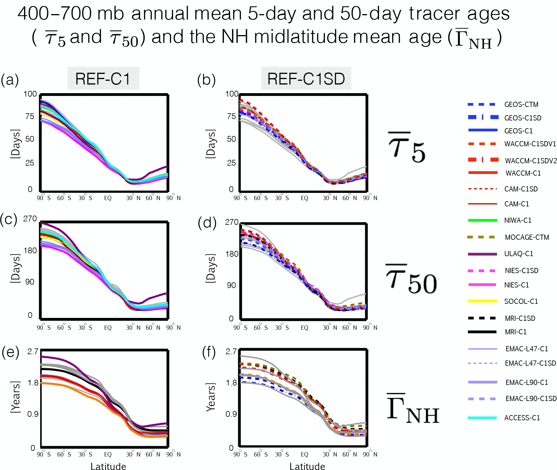
Figure 9Meridional profiles of the annual mean 5-day loss and 50-day loss tracer ages, (a, b) and (c, d), as well as the annually averaged mean transit time since air was last at the NH midlatitude surface (e, f). Panels (a, c, e) and (b, d, f) show the tracer ages for the REF-C1 and REF-C1SD simulations, respectively. The grey lines denote the C1SD(C1) simulations in the left (right) panels in order to a provide a sense of the ensemble spread.
3.2 Interhemispheric transport
3.2.1 Differences in transport
We now compare different measures of interhemispheric transport among the models. As in Orbe et al. (2016) we recast the idealized loss tracer concentrations χ5 and χ50 in terms of “tracer ages” τ5 and τ50, where , Ω is the NH midlatitude source region ΩMID and T refers to the exponential decay timescales 5 days and 50 days, respectively. This is a common approach in oceanography and facilitates comparison with the NH midlatitude mean age ΓNH (Deleersnijder et al., 2001; Waugh and Hall, 2002).
Meridional profiles of the annually averaged τ5, τ50 and ΓNH reveal large differences among all of the tracer ages over the middle troposphere (300–600 mb; Fig. 9), with Southern Hemisphere (SH) values of τ5 ranging between 70 and 90 days, or ∼ 25 % of the multi-model mean, while the mean age ΓNH varies between 1.7 and 2.6 years, or about ∼ 40 % of the multi-model mean. The differences in the tracer ages among the simulations emerge primarily in the tropics and are more or less consistent among the different ages such that simulations that tend to have small values of τ5 (relative to the multi-model mean) also feature relatively small values of the mean age ΓNH. This indicates that the age tracer differences arise due to transport differences in the tropical and subtropical lower troposphere and not in response to differences in the lower stratosphere, to which the 5-day age tracer is insensitive.
Consistent with the results in Orbe et al. (2017) we find that the interhemispheric transport differences among the C1SD simulations are as large as the differences among the free-running C1 simulations. Interestingly, this applies not only to simulations constrained with MERRA analysis fields (i.e., GEOS-CTM, GEOS-C1SD, WACCM C1SDV1/V2 and CAM C1) but also simulations constrained with fields from ERA-Interim (i.e., CMAM-C1SD, MOCAGE-CTM and NIES-C1SD). For example, the mean age differs by ∼ 0.5 years between the MOCAGE-CTM and CMAM-C1SD simulations over the SH compared to only about 0.15 years between the GEOS-C1 and CMAM-C1 free-running simulations, despite substantial differences in the large-scale flow among those models.
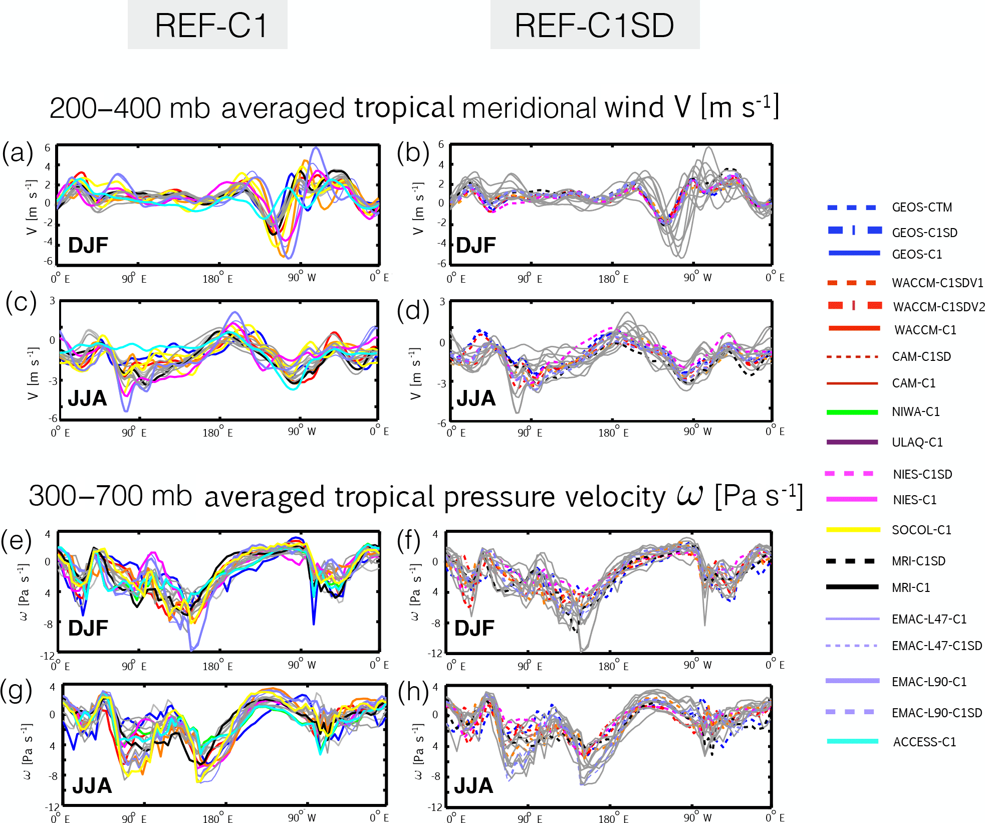
Figure 10Comparisons of the upper tropospheric meridional wind V (a–d) and 300–700 hPa averaged pressure velocity (e–h) among the simulations. The REF-C1 and REF-C1SD simulations are shown in panels (a, c, e, g) and (b, d, f, h), respectively. The grey lines denote the C1SD (C1) simulations in the left (right) panels in order to a provide a sense of the ensemble spread.
While ΓNH cannot be observed directly, Waugh et al. (2013) show that it can be approximated in terms of the time lag between the mixing ratio of sulfur hexafluoride (SF6) at a given location and the NH midlatitude surface. We have confirmed this finding among three of the CCMI simulations, for which both SF6 and ΓNH were output (not shown). Furthermore, comparisons with observational estimates of ΓNH, inferred in Waugh et al. (2013) from surface measurements of SF6, indicate that all of the CCMI models are older relative to the observations by 20–40 % for most of the models but up to 60 % for others. Due to the paucity of SF6 output among the models, however, we reserve a more detailed model–observation comparison for a future study.
3.2.2 Differences in tropical large-scale flow and parameterized convection
A possible source of differences in interhemispheric transport among the C1SD simulations are differences in the analysis fields themselves, which can differ significantly among reanalysis products (Stachnik and Schumacher, 2011). A comparison of the large-scale flow in the tropics reveals larger differences among the C1 simulations, in which we have approximated the tropical meridional circulation in terms of the meridional and vertical components of the velocity field (Fig. 10). This applies both to comparisons of the upper tropospheric meridional flow (V; Fig. 10a–d) and comparisons of the pressure velocity (ω) among the simulations, although the differences in ω among the C1SD simulations are by no means negligible (Fig. 10e–h). Furthermore, the differences among the NCAR and NASA C1SD simulations are small, despite the fact that the differences in the mean age ΓNH among those simulations span most of the ensemble spread (Fig. 9). Overall this suggests that the interhemispheric transport differences among the simulations are not driven primarily by differences in the large-scale flow.
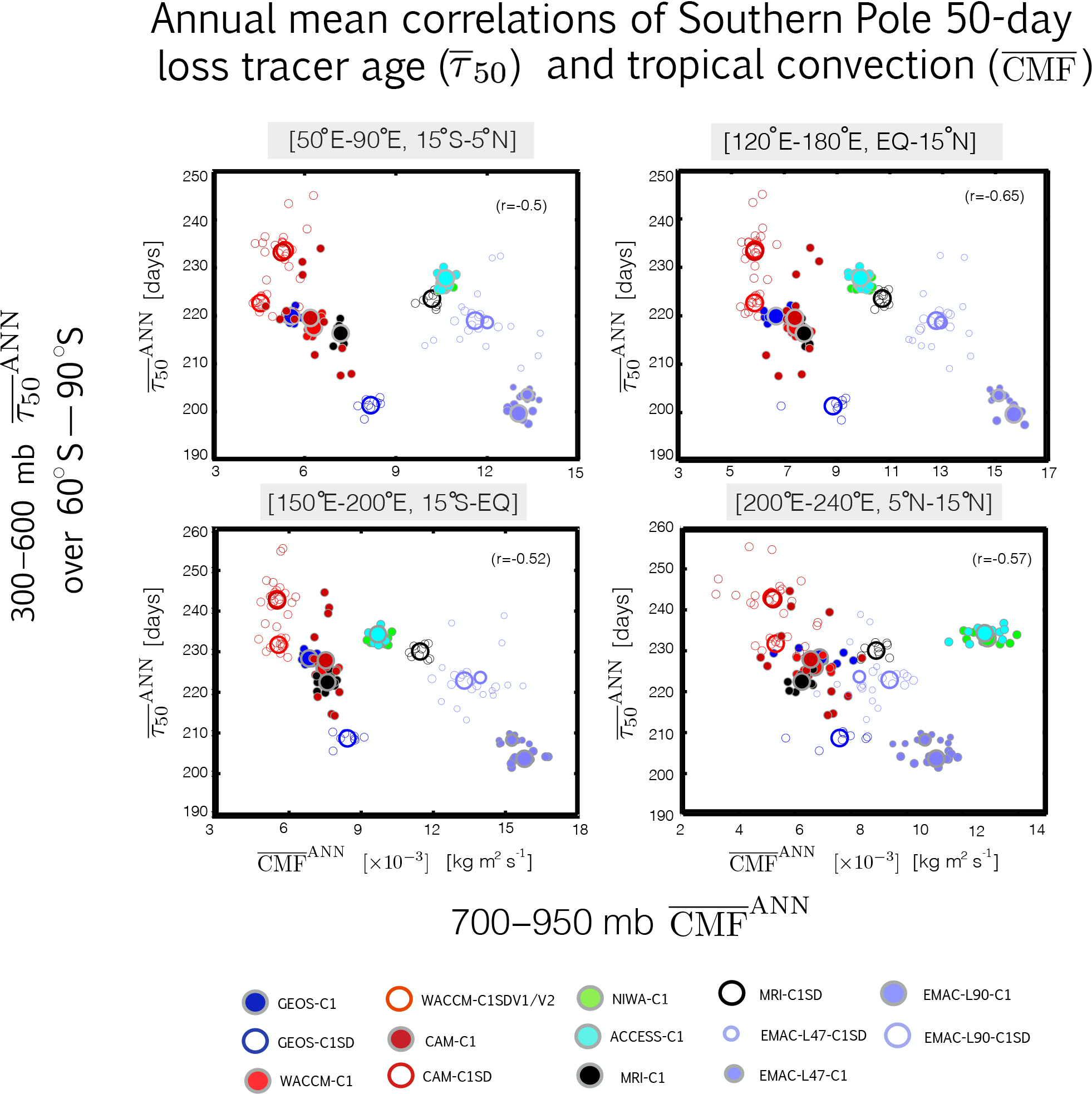
Figure 11Scatterplots showing negative correlations between the strength of parameterized convection in the tropics, represented by the 700–900 hPa averaged convective mass flux (), and mid-tropospheric (300–600 mb) values of the 50-day idealized loss tracer age, , evaluated over the Southern Pole. The different colors correspond to the different simulations, with open circles denoting REF-C1SD simulations and closed circles corresponding to REF-C1 free-running simulations. Small circles correspond to individual years within the 2000–2009 climatological mean period, while large circles denote the climatological mean.
Rather, Orbe et al. (2017) show that differences in interhemispheric transport between the NASA and NCAR C1SD simulations are more likely related to differences in convection over the northern subtropical oceans. We test this result among all the CCMI models and expand our region of interest to also include latitudes in the deep tropics, in accordance with previous studies showing that deep tropical convection significantly enhances interhemispheric transport (Gilliland and Hartley, 1998).
Among the CCMI ensemble we find strong correlations between annually averaged lower tropospheric (700–900 mb) convection over the tropical oceans and Southern Hemisphere tracer ages averaged poleward of 60∘ S (Fig. 11). Consistent with large differences in interhemispheric transport among the C1SD simulations, Fig. 11 reveals large differences in parameterized convection among simulations constrained with analysis fields. Furthermore, note that while the correlations are shown for the annual mean, we have performed a similar analysis accounting for seasonal variations in convection. That analysis reveals similar (if stronger) correlations (not shown).
Comparisons of idealized tracers among the CCMI hindcast simulations reveal large differences in their global-scale tropospheric transport properties, in particular the following.
-
There are large (30–40 %) differences in the efficiency of transport from the Northern Hemisphere midlatitude surface into the Arctic. To first order, these differences reflect differences in (parameterized) convection over the northern midlatitude oceans, particularly during boreal winter.
-
There are large differences in interhemispheric transport from northern midlatitudes to southern high latitudes, where the mean age ΓNH ranges between 1.7 and 2.6 years. In general, stronger tropical and subtropical convection is associated with faster interhemispheric transport.
-
The large-scale transport differences among simulations constrained with analyzed winds are as large as the differences among simulations using internally generated meteorological fields, which is consistent with the findings in Orbe et al. (2017). This is most likely related to large differences in (parameterized) convection among specified dynamics simulations, in addition to differences in the large-scale tropical flow.
Our findings suggest that differences in parameterized convection over the oceans are the primary drivers of transport differences among the CCMI simulations. By comparison, the differences related to how the large-scale flow is specified (e.g., CTM vs. nudging or source of analysis fields) appear to be relatively smaller. Therefore, our results indicate that caution should be taken when using the C1SD simulations to interpret the influence of meteorology on tropospheric composition. In the future more attention will need to be paid to understanding both how the large-scale flow is specified and the behavior of convective parameterizations in simulations constrained with analyzed winds, both in offline (CTM) and online (nudged) frameworks.
At this point it is not clear why the convection differences among the C1SD simulations are in certain cases larger than among free-running simulations using the same models. One possibility is that these differences arise due to inconsistencies (e.g., in resolution or unbalanced dynamics) between the driving large-scale flow fields and the convective mass fluxes, which are recalculated online in all of the nudged simulations and in the MOCAGE-CTM or interpolated directly from analysis fields (e.g., GEOS-CTM). The analysis in this study has been limited by the small number of C1SD simulations that output all of the idealized tracers and convective mass fluxes (Table 3). Experiments using multiple sources of analysis fields and different convective parameterizations will need to be performed in order to examine this problem more carefully. A review of the CCMI C1SD simulations, with details on how these simulations were constrained, is also currently in preparation and may provide further insight.
One important caveat in this study is that our focus has been on tracers with zonally uniform boundary conditions. The implications of our findings will therefore vary among different species, depending on where they are emitted over the Earth's surface. In particular, our results highlight the differences in transport that arise due to large differences in (parameterized) oceanic convection among the simulations. We anticipate, therefore, that our results will primarily apply to species with oceanic sources, including marine-sourced volatile organic compounds and short-lived ozone-depleting halogenated species. By comparison, species with primarily land emissions (e.g., short-lived species) are expected to be more sensitive to other aspects of transport. To this end, a study is currently in preparation that addresses the implications of biases in the latitude of the midlatitude jet on carbon monoxide distributions over the Arctic among the CCMI models. We reserve further discussions for that study.
Finally, while we have shown that there are large differences in transport among the models, we have not made comparisons with observations. As mentioned in Sect. 3.2.1, estimates of ΓNH inferred from surface measurements of SF6 (Waugh et al., 2013) indicate that all of the CCMI models are old compared to the observations. More recently, Holzer and Waugh (2015) presented estimates of both the mean age and the spectral width of the underlying transit-time distribution (TTD) connecting the NH midlatitude surface to the Southern Hemisphere based on surface measurements of SF6 and various chlorofluorocarbons and their replacement gases. These additional estimates may provide important constraints on the idealized loss tracer distributions in the CCMI simulations to the extent that the loss tracers approximate different aspects of the TTD, as demonstrated in Orbe et al. (2016) for the case of one model. We reserve more comparisons with observational constraints for future work.
All data from CCMI-1 used in this study can be obtained through the British Atmospheric Data Centre (BADC) archive (ftp://ftp.ceda.ac.uk, last access: 15 October 2017). For instructions for access to both archives, see http://blogs.reading.ac.uk/ccmi/badc-data-access (last access: 8 May 2018).
The supplement related to this article is available online at: https://doi.org/10.5194/acp-18-7217-2018-supplement.
The authors declare that they have no conflict of interest.
This article is part of the special issue “Chemistry–Climate Modelling Initiative (CCMI) (ACP/AMT/ESSD/GMD inter-journal SI)”. It is not associated with a conference.
We thank the Centre for Environmental Data Analysis (CEDA) for hosting the
CCMI data archive. We acknowledge the modeling groups for making their
simulations available for this analysis and the joint WCRP SPARC/IGAC
Chemistry–Climate Model Initiative (CCMI) for organizing and coordinating
this model data analysis activity. In addition, Clara Orbe and Luke D. Oman want to
acknowledge
the high-performance computing resources provided by the NASA Center for
Climate Simulation (NCCS) and support from the NASA Modeling, Analysis
and Prediction (MAP) program. Hideharu Akiyoshi acknowledges the Environment Research and
Technology Development Fund of the Environmental Restoration and Conservation
Agency, Japan (2-1709) and NECSX9/A(ECO) computers at CGER, NIES. Olaf Morgenstern and
Guang Zeng acknowledge the UK Met Office for use of the MetUM. Their research was
supported by the NZ government's Strategic Science Investment Fund (SSIF)
through the NIWA program CACV. Olaf Morgenstern acknowledges funding by the New Zealand
Royal Society Marsden Fund (grant 12-NIW-006) and by the Deep South National
Science Challenge (http://www.deepsouthchallenge.co.nz). Olaf Morgenstern and Guang Zeng
also wish to acknowledge the contribution of the NeSI high-performance computing
facilities to the results of this research. New Zealand's national facilities
are provided by the New Zealand eScience Infrastructure (NeSI) and funded
jointly by NeSI's collaborator institutions and through the Ministry of
Business, Innovation and Employment's Research Infrastructure program
(https://www.nesi.org.nz). Darryn W. Waugh acknowledges support from NSF grant
AGS-1403676 and NASA grant NNX14AP58G. The EMAC model simulations have been
performed at the German Climate Computing Centre (DKRZ) through support from
the Bundesministerium für Bildung und Forschung (BMBF). DKRZ and its
scientific steering committee are gratefully acknowledged for providing the
HPC and data archiving resources for the consortial project ESCiMo (Earth
System Chemistry integrated Modeling). Eugene Rozanov and Timofei Sukhodolov acknowledge support from the
Swiss National Science Foundation under grant 200021169241 (VEC). Robyn Schofield and Kane A. Stone
acknowledge support from the Australian Research Council's Centre of Excellence
for Climate System Science (CE110001028), the Australian government's
National Computational Merit Allocation Scheme (q90) and the Australian Antarctic
science grant program (FoRCES 4012).
Edited by: Peter Hess
Reviewed by: two anonymous referees
Abalos, M., Randel, W. J., Kinnison, D. E., and Garcia, R. R.: Using the artificial tracer e90 to examine present and future UTLS tracer transport in WACCM, J. Atmos. Sci., 74, 3383–3403, 2017. a
Akiyoshi, H., Nakamura, T., Miyasaka, T., Shiotani, M., and Suzuki, M.: A nudged chemistry-climate model simulation of chemical constituent distribution at northern high-latitude stratosphere observed by SMILES and MLS during the 2009/2010 stratospheric sudden warming, Tellus B, 121, 1361–1380, 2016.
Arakawa, A.: The cumulus parameterization problem: Past, present, and future, J. Climate, 17, 2493–2525, 2004. a
Arakawa, A. and Schubert, W. H.: Interaction of a cumulus cloud ensemble with the large-scale environment, Part I, J. Atmos. Sci., 31, 674–701, 1974.
Bacmeister, J. T., Suarez, M. J., and Robertson, F. R.: Rain reevaporation, boundary layer–convection interactions, and Pacific rainfall patterns in an AGCM, J. Atmos. Sci., 63, 3383–3403, 2006.
Bechtold, P., Bazile, E., Guichard, F., Mascart, P., and Richard, E.: A mass-flux convection scheme for regional and global models, Q. J. Roy. Meteor. Soc., 127, 869–886, 2001.
Bowman, K. P. and Erukhimova, T.: Comparison of global-scale Lagrangian transport properties of the NCEP reanalysis and CCM3, J. Climate, 17, 1135–1146, 2004. a
Deleersnijder, E., Campin, J.-M., and Delhez, E. J.: The concept of age in marine modelling: I. theory and preliminary model results, J. Mar. Syst., 28, 229–267, 2001. a
Denning, A. S., Holzer, M., Gurney, K. R., Heimann, M., Law, R. M., Rayner, P. J., Fung, I. Y., Fan, S.-M., Taguchi, S., and Friedlingstein, P.: Three-dimensional transport and concentration of SF6, Tellus B, 51, 266–297, 1999. a, b
Deushi, S. and Shibata, K.: Development of a Meteorological Research Institute Chemistry-Climate Model version 2 for the study of tropospheric and stratospheric chemistry, Pap. Meteorol. Geophys., 62, 1–46, 2011.
Eckhardt, S., Stohl, A., Beirle, S., Spichtinger, N., James, P., Forster, C., Junker, C., Wagner, T., Platt, U., and Jennings, S. G.: The North Atlantic Oscillation controls air pollution transport to the Arctic, Atmos. Chem. Phys., 3, 1769–1778, https://doi.org/10.5194/acp-3-1769-2003, 2003. a
Eckhardt, S., Stohl, A., Wernli, H., James, P., Forster, C., and Spichtinger, N.: A 15-year climatology of warm conveyor belts, J. Climate, 17, 218–237, 2004. a
Eyring, V., Lamarque, J.-F., Hess, P., Arfeuille, F., Bowman, K., Chipperfiel, M. P., Duncan, B., Fiore, A., Gettelman, A., and Giorgetta, M. A. : Overview of IGAC/SPARC Chemistry-Climate Model Initiative (CCMI) community simulations in support of upcoming ozone and climate assessments, SPARC newsletter, 40, 48–66, 2013. a
Forster, C., Stohl, A., and Seibert, P.: Parameterization of convective transport in a lagrangian particle dispersion model and its evaluation, J. Appl. Meteorol. Clim., 46, 403–422, 2007. a
Garcia, R., Smith, A., Kinnison, D., de la Cámara, A., and Murphy, D.: Modification of the gravity wave parameterization in the Whole Atmosphere Community Climate Model: Motivation and results, J. Atmos. Sci., 74, 275–291, 2017.
Gilliland, A. and Hartley, D.: Interhemispheric transport and the role of convective parameterizations, J. Geophys. Res.-Atmos., 103, 22039–22045, 1998. a
Grewe, V., Brunner, D., Dameris, M., Grenfell, J. L., Hein, R., Shindell, D., and Staehelin, J.: Origin and variability of upper tropospheric nitrogen oxides and ozone at northern mid-latitudes, Atmos. Environ., 35, 3421–3433, 2001.
Guth, J., Josse, B., Marécal, V., Joly, M., and Hamer, P.: First implementation of secondary inorganic aerosols in the MOCAGE version R2.15.0 chemistry transport model, Geosci. Model Dev., 9, 137–160, https://doi.org/10.5194/gmd-9-137-2016, 2016.
Hack, J. J., Boville, B. A., Kiehl, J. T., Rasch, P. J., and Williamson, D. L.: Climate statistics from the National Center for Atmospheric Research community climate model CCM2, J. Geophys. Res.-Atmos., 99, 20785–20813, 1994.
Hewitt, H. T., Copsey, D., Culverwell, I. D., Harris, C. M., Hill, R. S. R., Keen, A. B., McLaren, A. J., and Hunke, E. C.: Design and implementation of the infrastructure of HadGEM3: the next-generation Met Office climate modelling system, Geosci. Model Dev., 4, 223–253, https://doi.org/10.5194/gmd-4-223-2011, 2011.
Holzer, M.: Analysis of passive tracer transport as modeled by an atmospheric general circulation model, J. Climate, 12, 1659–1684, 1999. a
Holzer, M. and Waugh, D. W.: Interhemispheric transit time distributions and path-dependent lifetimes constrained by measurements of SF6, CFCs, and CFC replacements, Geophys. Res. Lett., 42, 4581–4589, 2015. a
Hoskins, B. J.,Towards a PV-Θ view of the general circulation, Tellus A, 43, 27–35, 1991. a
Imai, K., Manago, N., Mitsuda, C., Naito, Y., Nishimoto, E., Sakazaki, T., Fujiwara, M., Froidevaux, L., Clarmann, T., Stiller, G. P., and Murtagh, D. P.: Validation of ozone data from the Superconducting Submillimeter-Wave Limb-Emission Sounder (SMILES), J. Geophys. Res.-Atmos., 118, 5750–5769, 2013.
Jöckel, P., Kerkweg, A., Pozzer, A., Sander, R., Tost, H., Riede, H., Baumgaertner, A., Gromov, S., and Kern, B.: Development cycle 2 of the Modular Earth Submodel System (MESSy2), Geosci. Model Dev., 3, 717–752, https://doi.org/10.5194/gmd-3-717-2010, 2010.
Jöckel, P., Tost, H., Pozzer, A., Kunze, M., Kirner, O., Brenninkmeijer, C. A. M., Brinkop, S., Cai, D. S., Dyroff, C., Eckstein, J., Frank, F., Garny, H., Gottschaldt, K.-D., Graf, P., Grewe, V., Kerkweg, A., Kern, B., Matthes, S., Mertens, M., Meul, S., Neumaier, M., Nützel, M., Oberländer-Hayn, S., Ruhnke, R., Runde, T., Sander, R., Scharffe, D., and Zahn, A.: Earth System Chemistry integrated Modelling (ESCiMo) with the Modular Earth Submodel System (MESSy) version 2.51, Geosci. Model Dev., 9, 1153–1200, https://doi.org/10.5194/gmd-9-1153-2016, 2016.
Jonsson, A., Grandpre, J., Fomichev, V., McConnell, J., and Beagley, S.: Doubled CO2-induced cooling in the middle atmosphere: Photochemical analysis of the ozone radiative feedback, J. Geophys. Res.-Atmos., 109, D24103, https://doi.org/10.1029/2004JD005093, 2004.
Josse, B., Simon, P., and Peuch, V. H.: Radon global simulations with the multiscale chemistry and transport model MOCAGE, Tellus B, 56, 339–356, 2004.
Klonecki, A., Hess, P., Emmons, L., Smith, L., Orlando, J., and Blake, D.: Seasonal changes in the transport of pollutants into the arctic troposphere–model study, J. Geophys. Res.-Atmos., 108, 8367, https://doi.org/10.1029/2002JD002199, 2003. a, b, c
Lamarque, J.-F., Shindell, D. T., Josse, B., Young, P. J., Cionni, I., Eyring, V., Bergmann, D., Cameron-Smith, P., Collins, W. J., Doherty, R., Dalsoren, S., Faluvegi, G., Folberth, G., Ghan, S. J., Horowitz, L. W., Lee, Y. H., MacKenzie, I. A., Nagashima, T., Naik, V., Plummer, D., Righi, M., Rumbold, S. T., Schulz, M., Skeie, R. B., Stevenson, D. S., Strode, S., Sudo, K., Szopa, S., Voulgarakis, A., and Zeng, G.: The Atmospheric Chemistry and Climate Model Intercomparison Project (ACCMIP): overview and description of models, simulations and climate diagnostics, Geosci. Model Dev., 6, 179–206, https://doi.org/10.5194/gmd-6-179-2013, 2013. a
Lin, M., Fiore, A. M., Horowitz, L. W., Langford, A. O., Oltmans, S. J., Tarasick, D., and Rieder, H. E.: Climate variability modulates western US ozone air quality in spring via deep stratospheric intrusions, Nat. Commun., 6, 7105, https://doi.org/10.1038/ncomms8105, 2015. a
Liu, C. and Barnes, E. A.: Extreme moisture transport into the arctic linked to rossby wave breaking, J. Geophys. Res.-Atmos., 120, 3774–3788, 2015. a
Mahlman, J.: Dynamics of transport processes in the upper troposphere, Science, 276, 1079–1083, 1997. a
Marsh, D. R., Mills, M. J., Kinnison, D. E., Lamarque, J.-F., Calvo, N., and Polvani, L. M.: Climate change from 1850 to 2005 simulated in CESM1 (WACCM), J. Climate, 26, 7372–7391, 2013. a
Molod, A., Takacs, L., Suarez, M., and Bacmeister, J.: Development of the GEOS-5 atmospheric general circulation model: evolution from MERRA to MERRA2, Geosci. Model Dev., 8, 1339–1356, https://doi.org/10.5194/gmd-8-1339-2015, 2015. a
Moorthi, S. and Suarez, M. J.: Relaxed Arakawa-Schubert. A parameterization of moist convection for general circulation models, Mon. Weather Rev., 120, 978–1002, 1992.
Morgenstern, O., Braesicke, P., O'Connor, F. M., Bushell, A. C., Johnson, C. E., Osprey, S. M., and Pyle, J. A.: Evaluation of the new UKCA climate-composition model – Part 1: The stratosphere, Geosci. Model Dev., 2, 43–57, https://doi.org/10.5194/gmd-2-43-2009, 2009.
Morgenstern, O., Zeng, G., Abraham, L., Telford, P., Braesicke, P., Pyle, J., Hardiman, S., O'Connor, F., and Johnson, C.: Impacts of climate change, ozone recovery, and increasing methane on surface ozone and the tropospheric oxidizing capacity J. Geophys. Res.-Atmos., 118, 1028–1041, 2013.
Morgenstern, O., Hegglin, M. I., Rozanov, E., O'Connor, F. M., Abraham, N. L., Akiyoshi, H., Archibald, A. T., Bekki, S., Butchart, N., Chipperfield, M. P., Deushi, M., Dhomse, S. S., Garcia, R. R., Hardiman, S. C., Horowitz, L. W., Jöckel, P., Josse, B., Kinnison, D., Lin, M., Mancini, E., Manyin, M. E., Marchand, M., Marécal, V., Michou, M., Oman, L. D., Pitari, G., Plummer, D. A., Revell, L. E., Saint-Martin, D., Schofield, R., Stenke, A., Stone, K., Sudo, K., Tanaka, T. Y., Tilmes, S., Yamashita, Y., Yoshida, K., and Zeng, G.: Review of the global models used within phase 1 of the Chemistry–Climate Model Initiative (CCMI), Geosci. Model Dev., 10, 639–671, https://doi.org/10.5194/gmd-10-639-2017, 2017. a, b, c
Nordeng, T. E.: Extended versions of the convective parametrization scheme at ECMWF and their impact on the mean and transient activity of the model in the tropics, Research Department Technical Memorandum, 206, 1–41, ECMWF, Shinfield Park, Reading, UK, 1994.
Orbe, C., Newman, P. A., Waugh, D. W., Holzer, M., Oman, L. D., Li, F., and Polvani, L. M.: Air-mass origin in the Arctic. Part I: Seasonality, J. Climate, 28, 4997–5014, 2015. a
Orbe, C., Waugh, D. W., Newman, P. A., and Steenrod, S.: The transit-time distribution from the Northern Hemisphere midlatitude surface, J. Atmos. Sci., 73, 3785–3802, 2016. a, b, c, d
Orbe, C., Waugh, D. W., Yang, H., Lamarque, J. F., Tilmes, S., and Kinnison, D. E.: Tropospheric transport differences between models using the same large-scale meteorological fields, Geophys. Res. Lett., 44, 1068–1078, 2017. a, b, c, d, e, f, g, h, i, j, k, l
Patra, P. K., Houweling, S., Krol, M., Bousquet, P., Belikov, D., Bergmann, D., Bian, H., Cameron-Smith, P., Chipperfield, M. P., Corbin, K., Fortems-Cheiney, A., Fraser, A., Gloor, E., Hess, P., Ito, A., Kawa, S. R., Law, R. M., Loh, Z., Maksyutov, S., Meng, L., Palmer, P. I., Prinn, R. G., Rigby, M., Saito, R., and Wilson, C.: TransCom model simulations of CH4 and related species: linking transport, surface flux and chemical loss with CH4 variability in the troposphere and lower stratosphere, Atmos. Chem. Phys., 11, 12813–12837, https://doi.org/10.5194/acp-11-12813-2011, 2011. a, b
Pitari, G., Aquila, V., Kravitz, B., Robock, A., Watanabe, S., Cionni, I., Luca, N., Genova, G., Mancini, E., and Tilmes, S.: Stratospheric ozone response to sulfate geoengineering: Results from the Geoengineering Model Intercomparison Project (GeoMIP), J. Geophys. Res.-Atmos., 119, 2629–2653, 2014.
Prather, M., McElroy, M., Wofsy, S., Russell, G., and Rind, D.: Chemistry of the global troposphere: Fluorocarbons as tracers of air motion, J. Geophys. Res.-Atmos., 92, 6579–6613, 1987. a
Prather, M. J., Zhu, X., Tang, Q., Hsu, J., and Neu, J. L.: An atmospheric chemist in search of the tropopause, J. Geophys. Res.-Atmos., 116, D04306, https://doi.org/10.1029/2010JD014939, 2011. a
Reinecker, M., Suarez, M., Todling, R., Bacmeister, J., Takacs, L., Liu, H., Gu, W., Sienkiewicz, M., Koster, R., Gelaro, R., and Stajner, I.: The geos-5 data assimilation system: A documentation of geos-5.0, NASA Tech. Rep, 104606, V27, available at: https://gmao.gsfc.nasa.gov/pubs/docs/GEOS-5.0.1_Documentation_r3.pdf (last access: 4 May 2018), 2007. a
Revell, L. E., Tummon, F., Stenke, A., Sukhodolov, T., Coulon, A., Rozanov, E., Garny, H., Grewe, V., and Peter, T.: Drivers of the tropospheric ozone budget throughout the 21st century under the medium-high climate scenario RCP 6.0, Atmos. Chem. Phys., 15, 5887–5902, https://doi.org/10.5194/acp-15-5887-2015, 2015.
Rienecker, M. M., Suarez, M. J., Gelaro, R., Todling, R., Bacmeister, J., Liu, E., Bosilovich, M. G., Schubert, S. D., Takacs, L., Kim, G.-K., Bloom, S.: MERRA: NASA's modern-era retrospective analysis for research and applications, J. Climate, 24, 3624–3648, 2011. a
Scinocca, J. F., McFarlane, N. A., Lazare, M., Li, J., and Plummer, D.: Technical Note: The CCCma third generation AGCM and its extension into the middle atmosphere, Atmos. Chem. Phys., 8, 7055–7074, https://doi.org/10.5194/acp-8-7055-2008, 2008.
Shindell, D. T., Chin, M., Dentener, F., Doherty, R. M., Faluvegi, G., Fiore, A. M., Hess, P., Koch, D. M., MacKenzie, I. A., Sanderson, M. G., Schultz, M. G., Schulz, M., Stevenson, D. S., Teich, H., Textor, C., Wild, O., Bergmann, D. J., Bey, I., Bian, H., Cuvelier, C., Duncan, B. N., Folberth, G., Horowitz, L. W., Jonson, J., Kaminski, J. W., Marmer, E., Park, R., Pringle, K. J., Schroeder, S., Szopa, S., Takemura, T., Zeng, G., Keating, T. J., and Zuber, A.: A multi-model assessment of pollution transport to the Arctic, Atmos. Chem. Phys., 8, 5353–5372, https://doi.org/10.5194/acp-8-5353-2008, 2008. a
Solomon, S., Kinnison, D., Bandoro, J., and Garcia, R.: Simulation of polar ozone depletion: An update, J. Geophys. Res.-Atmos., 120, 7958–7974, 2015.
SPARC CCMVal: Chemistry–Climate Model validation, SPARC Report No. 5, WCRP-30, WMO/TD-No. 40, available at: http://www.sparc-climate.org/publications/sparc-reports/sparc-report-no-5/ (last access: 9 May 2018), 2010. a
Stachnik, J. P. and Schumacher, C.: A comparison of the Hadley circulation in modern reanalyses, J. Geophys. Res.-Atmos., 116, D22102, https://doi.org/10.1029/2011JD016677, 2011. a
Stenke, A., Schraner, M., Rozanov, E., Egorova, T., Luo, B., and Peter, T.: The SOCOL version 3.0 chemistry–climate model: description, evaluation, and implications from an advanced transport algorithm, Geosci. Model Dev., 6, 1407–1427, https://doi.org/10.5194/gmd-6-1407-2013, 2013.
Stohl, A.: Characteristics of atmospheric transport into the arctic troposphere, J. Geophys. Res.-Atmos., 111, D11306, https://doi.org/10.1029/2005JD006888, 2006. a
Stone, K. A., Morgenstern, O., Karoly, D. J., Klekociuk, A. R., French, W. J., Abraham, N. L., and Schofield, R.: Evaluation of the ACCESS – chemistry–climate model for the Southern Hemisphere, Atmos. Chem. Phys., 16, 2401–2415, https://doi.org/10.5194/acp-16-2401-2016, 2016.
Strahan, S., Douglass, A., and Newman, P.: The contributions of chemistry and transport to low arctic ozone in march 2011 derived from aura mls observations, J. Geophys. Res.-Atmos., 118, 1563–1576, 2013. a, b
Tiedtke, M.: A comprehensive mass flux scheme for cumulus parameterization in large-scale models, Mon. Weather Rev., 117, 1779–1800, 1989. a
Tilmes, S., Lamarque, J.-F., Emmons, L. K., Kinnison, D. E., Ma, P.-L., Liu, X., Ghan, S., Bardeen, C., Arnold, S., Deeter, M., Vitt, F., Ryerson, T., Elkins, J. W., Moore, F., Spackman, J. R., and Val Martin, M.: Description and evaluation of tropospheric chemistry and aerosols in the Community Earth System Model (CESM1.2), Geosci. Model Dev., 8, 1395–1426, https://doi.org/10.5194/gmd-8-1395-2015, 2015.
Waugh, D. W. and Hall, T. M.: Age of stratospheric air: Theory, observations, and models, Rev. Geophys., 40, 1010, https://doi.org/10.1029/2000RG000101, 2002. a
Waugh, D. W., Crotwell, A. M., Dlugokencky, E. J., Dutton, G. S., Elkins, J. W., Hall, B. D., Hintsa, E. J., Hurst, D. F., Montzka, S. A., Mondeel, D. J., and Moore, F. L.: Tropospheric SF6: Age of air from the Northern Hemisphere midlatitude surface, J. Geophys. Res.-Atmos., 118, 11–429, 2013. a, b, c, d, e
Yang, H., Waugh, D. W., and Orbe, C.: Tropospheric Midlatitude-to-Arctic Transport of a CO-like Tracer in the Chemistry Climate Model Initiative (CCMI) Simulations, in preparation, 2018. a
Yoshimura, H., Mizuta, R., and Murakami, H.: A spectral cumulus parameterization scheme interpolating between two convective updrafts with semi-Lagrangian calculation of transport by compensatory subsidence, Mon. Weather Rev., 143, 597–621, 2015.
Yukimoto, S.: Meteorological research institute earth system model version 1 (MRI-ESM1): model description, Meteorological Research Institute, available at: http://www.mri-jma.go.jp/Publish/Technical/DATA/VOL_64/tec_rep_mri_64.pdf (last access: 9 May 2018), 2011.
Yukimoto, S., Adachi, Y., Hosaka, M., Sakami, T., Yoshimura, H., Hirabara, M., Tanaka, T. Y., Shindo, E., Tsujino, H., Deushi, M., and Mizuta, R.: A new global climate model of the Meteorological Research Institute: MRI-CGCM3 model description and basic performance, J. Meteorol. Soc. Jpn. Ser. II, 90, 23–64, 2012.
Zhang, G. J. and McFarlane, N. A.: Sensitivity of climate simulations to the parameterization of cumulus convection in the Canadian Climate Centre general circulation model, Atmos. Ocean, 33, 407–446, 1995.
Zhang, K., Wan, H., Zhang, M., and Wang, B.: Evaluation of the atmospheric transport in a GCM using radon measurements: sensitivity to cumulus convection parameterization, Atmos. Chem. Phys., 8, 2811–2832, https://doi.org/10.5194/acp-8-2811-2008, 2008. a