the Creative Commons Attribution 4.0 License.
the Creative Commons Attribution 4.0 License.
 | 09 May 2018
LES study of the impact of moist thermals on the oxidative capacity of the atmosphere in southern West Africa
Fabien Brosse
Maud Leriche
Céline Mari
Fleur Couvreux
The hydroxyl radical (OH) is a highly reactive species and plays a key role in the oxidative capacity of the atmosphere. We explore the potential impact of a convective boundary layer on reconciling the calculation–measurement differences for OH reactivity (the inverse of OH lifetime) attributable to the segregation of OH and its reactants by thermals and the resulting modification of averaged reaction rates. The large-eddy simulation version of the Meso-NH model is used, coupled on-line with a detailed chemistry mechanism to simulate two contrasted biogenic and urban chemical regimes. In both environments, the top of the boundary layer is the region with the highest calculated segregation intensities but with the opposite sign. In the biogenic environment, the inhomogeneous mixing of isoprene and OH leads to a maximum decrease of 30 % of the mean reaction rate in this zone. In the anthropogenic case, the effective rate constant for OH reacting with aldehydes is 16 % higher than the averaged value. OH reactivity is always higher by 15 to 40 % inside thermals in comparison to their surroundings as a function of the chemical environment and time of the day. Since thermals occupy a small fraction of the simulated domain, the impact of turbulent motions on domain-averaged total OH reactivity reaches a maximum decrease of 9 % for the biogenic case and a maximum increase of 5 % for the anthropogenic case. Accounting for the segregation of air masses by turbulent motions in regional and global models may increase OH reactivity in urban environments but lower OH reactivity in biogenic environments. In both cases, segregation alone is insufficient for resolving the underestimation between observed and modeled OH reactivity.
- Article
(5147 KB) - Full-text XML
- BibTeX
- EndNote


The hydroxyl radical (OH) is an efficient cleansing molecule present in the troposphere. It is mainly produced during the daytime through the reaction of water vapor with O(1D), formed by ozone photolysis, while nitrogen oxides and volatile organic compounds (VOCs) are its major sinks. OH is highly reactive and reacts with numerous chemical species, controlling their chemical lifetimes (Ehhalt, 1999). Both OH concentrations and OH reactivity are key elements of the oxidative capacity of the atmosphere.
Several field campaigns have been conducted to study total OH reactivity for urban and forested environments. Measured reactivities have been compared to calculated reactivities obtained by summing OH reactant concentrations and multiplying them by their reaction rate constants. A missing part, corresponding to the difference between measured and calculated OH reactivity, is found not only under urban or biogenic conditions but also in clean remote regions. Measured OH reactivity in urban areas has been shown to be similar (less than 10 %) to calculated OH reactivity in New York (Ren, 2003), in Houston (Mao et al., 2010) and in a controlled urban environment (Hansen et al., 2015). However, discrepancies in urban areas have been observed between measured and calculated OH reactivity in Nashville (Kovacs et al., 2003) (35 % less for calculated reactivity), in Mexico (Shirley et al., 2006) (25 %) and in Tokyo (Sadanaga, 2004) (25 %). The differences between measured and calculated total OH reactivity are even higher in forested areas. Di Carlo (2004) found an unexplained fraction of 50 % in measured OH reactivity during the PROPHET campaign in Michigan. These results are comparable to the missing part (50 to 58 %) calculated from measurements made in a boreal forest in Finland (Sinha et al., 2010; Nölscher et al., 2012). Similarly, Nölscher et al. (2016) calculated an accounted fraction of measured OH reactivity close to 49 % in an Amazonian rainforest.
As shown by Williams and Brune (2015), atmospheric models do not correctly simulate observed total OH reactivity. Attempts to use numerical models to explain the missing fraction of OH reactivity have proved to be insufficient. Indeed, Edwards et al. (2013) found an underestimation of 30 % of OH reactivity in a box model with a detailed chemical mechanism for the OP3 project. In the PRIDE-PRD campaign, Lou et al. (2010) found discrepancies of ±10 % between the results of the OH reactivity model and the measurements, also using a box model. Similarly, Mogensen et al. (2011) used a column model to elucidate the missing part of OH reactivity, but only explained 30 to 50 % of the OH reactivity measured over a forest in Finland. Chatani et al. (2009) used a three-dimensional model with coarse resolution to fill the gap in OH reactivity but 40 % of the measured OH sinks remained unexplained. The difficulty of getting models to represent OH reactivity could be partly due to as yet nondiscovered OH reaction pathways, which are therefore not implemented in atmospheric models. OH recycling by the isoprene oxidation chain in forest environments characterized by low NOx (sum of NO and NO2) conditions (i.e., < 1 ppb) was proposed to explain the uncertainties in the simulated HOx (sum of OH and HO2) budget (Lelieveld et al., 2008; Butler et al., 2008; Peeters et al., 2009; Pugh et al., 2010; Stone et al., 2011).
However, Stone et al. (2011) studied several proposed OH recycling mechanisms present in the literature and found that biases from OH and HO2 concentrations still exist whatever the mechanism.
One possible issue in total OH reactivity retrieval not mentioned by previous studies could lie in neglecting turbulent motions in the transport of chemical compounds in the boundary layer. Indeed, turbulence can spatially segregate or bring together chemical species, reducing or increasing the mean reaction rate and thus chemical reactivity. However, as far as we know this physical process has not been investigated in previous studies. The time response of current OH reactivity measurement techniques is not yet sufficient to directly resolve the smallest relevant turbulent spatial scales. The limitations in time resolutions range from 30 seconds for LIF-based methods (Kovacs and Brune, 2001; Sadanaga, 2004) to 1 min for the CRM method (Sinha et al., 2008). In comparison, Pugh et al. (2011) and Dlugi et al. (2010) used direct isoprene and OH concentrations measurements with temporal resolution of a few seconds, fast enough to estimate the segregation of the compounds.
The atmospheric boundary layer has a turbulent structure characterized by strong and narrow updrafts surrounded by weak and large descending areas (Molemaker and Vilà-Guerau de Arellano, 1998; Schumann, 1989). Wyngaard and Brost (1984) considered passive scalars and found that surface bottom-up transport plays a more important role in the vertical diffusion than the entrainment zone top-down transport in a convective boundary layer. Updrafts in the boundary layer lead to the spatial discrimination of pollutant concentrations between thermals and their environment. This heterogeneity in chemical species redistribution influences the mean reaction rate obtained when considering averaged reactant concentrations (Vilà-Guerau de Arellano and Cuijpers, 2000). Using an idealized simulation, Molemaker and Vilà-Guerau de Arellano (1998) showed that, for a second-order reaction implying a top-down and a bottom-up species, reaction rates are maximum in updrafts near the surface and in downdrafts at the top of the boundary layer. Segregation between the VOC and the OH radical was first addressed by the numerical study of Krol et al. (2000), who investigated the turbulence effects on the mean reaction rates of these species. Ouwersloot et al. (2011) studied the inefficiency of turbulent mixing over heterogeneous surfaces and found that the highest reaction rates for isoprene and OH are located in thermals at the top of the boundary layer. The chemical reactivity of the boundary layer is therefore determined by the capacity of turbulence to mix reactive species (Molemaker and Vilà-Guerau de Arellano, 1998). However, modeling and experimental studies investigating heterogeneities in the boundary layer have focused on OH radical concentrations rather than on OH reactivity due to the instrumental limitations discussed above.
Vertical motions associated with clouds and sea breezes impact the atmospheric chemistry and pollution levels near the surface since they dilute chemical species and increase the upward transport of surface emissions (Chen et al., 2012). In the case of updrafts leading to cloud formation, Vilà-Guerau de Arellano et al. (2005) found a decrease of 10 to 50 % of tracer mixing ratios averaged over the boundary layer with respect to a situation without clouds due to the deepening of the boundary layer. Clouds have multiple impacts on the atmospheric boundary layer as they induce turbulent mixing of chemical compounds which modifies reaction rates. They also modify incoming solar radiation, which in turn disturbs photolysis reactions and alters the emissions of biogenic compounds, such as isoprene. Finally, they alter atmospheric chemistry due to soluble gas washout and chemical reactions occurring in cloud droplets.
Cloud cover over West Africa is an important feature of the African monsoon but is poorly represented by global models (Knippertz et al., 2011; Hannak et al., 2017). This could lead to overly low simulated clouds and overly high incoming radiation at the surface, implying excessively high diurnal temperature and relative humidity cycles over this region. The nocturnal low-level stratus was studied during the monsoon period at Parakou (Benin) by Schrage et al. (2007) with radiosondes. The authors found that turbulent processes are responsible for cloudy nights, whereas clear nights are associated with a nocturnal inversion, leading to the decoupling of the surface and lower atmosphere. Schrage and Fink (2012) investigated nighttime cloud formation. They observed that the presence of a nighttime low-level jet induces the shear-driven vertical mixing of moisture accumulated near the surface. This leads to stratus formation whose cover is likely to persist until the early afternoon when it breaks up to form cumulus clouds (Schrage et al., 2007; Schrage and Fink, 2012). However, studying the impact of this specific cloudy environment on the turbulent transport of chemical species in tropical West Africa has not been reported.
High-resolution simulations which explicitly resolve the turbulent and convective advection terms were conducted (Vilà-Guerau de Arellano and Cuijpers, 2000; Vilà-Guerau de Arellano et al., 2005; Ouwersloot et al., 2011; Kim et al., 2012, 2016) to assess the impacts of clouds and the convective boundary layer on the mixing of chemical compounds. However, previous numerical studies on the impact of the turbulent mixing of chemical compounds mainly used relatively simple or only slightly more detailed chemical schemes (e.g., Vilà-Guerau de Arellano and Cuijpers, 2000,Vilà-Guerau de Arellano et al., 2005 and Ouwersloot et al., 2011), resulting in possible limitations in the representation of the atmospheric chemistry. Besides, more recent studies by Kim et al. (2012) and Kim et al. (2016) used a more detailed chemical scheme derived from Mozart v2.2, allowing the formation of OH radicals initiated by peroxy radicals. This limits the spatial heterogeneities caused by the reactions consuming the OH radical.
The goal of this work is to evaluate the role of thermals in OH reactivity in the framework of a convective boundary layer with contrasted chemical environments in southern West Africa. It focuses in particular on investigating turbulence as a possible explanation of the discrepancies between calculated and measured OH reactivities mentioned in the literature.
Two contrasted chemical regimes represented by a detailed chemical scheme are studied by using large-eddy simulations. The first simulation is influenced by biogenic emissions, whereas the second is characterized by anthropogenic emissions representative of Cotonou (Benin) in the center of the domain. Based on a conditional sampling implemented in the model, the thermals are discriminated in these simulations, allowing the specific chemical regime inside thermals to be investigated. The model experiments are presented in Sect. 2. Section 3 presents the dynamical and chemical results for the two cases while Sect. 4 presents the discussion relating to these results.
2.1 Model configuration
LES simulations are performed with the mesoscale nonhydrostatic atmospheric model Meso-NH (http://mesonh.aero.obs-mip.fr/mesonh/, last access: 26 April 2018) version 5.2.1, developed jointly by the Laboratoire d'Aérologie and the Centre National de la Recherche Météorologique (Lac et al., 2018). Cloud microphysical processes are represented by the ICE3 scheme (Pinty and Jabouille, 1998) that includes six different types of hydrometeors. The turbulence is solved by a three-dimensional scheme using a prognostic equation for the turbulent kinetic energy (Cuxart et al., 2000) with the turbulent mixing length given by the mesh size. Surface processes and interactions with the atmosphere are simulated by the SURFEx model (Masson et al., 2013) coupled with Meso-NH.
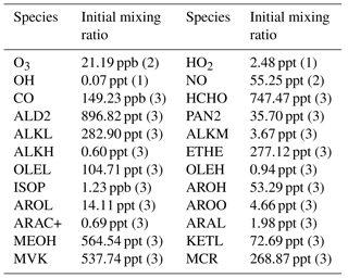
Table 1Initial vertical profiles of mixing ratios and associated profiles. Numbers in brackets refer to (1) uniform profile, (2) stratospheric profile (initial profile multiplied by 1 from 0 to 2000 m, then by 0.5 from 3000 m to 13 000 m, by 0.75 at 14 000 m and 1 above), (3) boundary layer profile (multiplied by 1 from 0 to 1000 m, by 0.10 from 2000 to 13 000 m and 0.05 above). Chemical names are those used in the ReLACS3 chemical mechanism. ALD2 corresponds to aldehydes C > 2, ALKL to lumped alkanes C2-C6, ALKM to lumped alkanes C7-C12, ALKH to lumped alkenes > C12, OLEH to lumped alkenes C > 6, ETHE to ethene, ISOP to isoprene, AROL to lumped low SOA yield aromatic species, AROH to lumped high SOA yield aromatic species, AROO to lumped phenolic species, ARAC+ to lumped aromatic monoacids, MEOH to methanol, ARAL to lumped aromatic monoaldehydes, MVK to methyl-vinyl-ketone, MCR to methacrolein, HCHO to formaldehyde, KETL to lumped ketones C3-C6 and PAN2 to peroxy acetyl nitrate
The resolution used is 50 m × 50 m for a domain size of 10 km × 10 km (200×200 grid points). 10 km is the targeted mesh size of an increasing number of current large-scale chemistry models. Along the vertical, 121 levels are stretched from Δz=20 m at the surface to 250 m on top of the domain at 20 km, and the boundary conditions are cyclic.
The simulation is run for 3 days, in which 2 days consist of the spin-up for chemistry. The same dynamical conditions and the same initial and forcing thermodynamical fields are used for each day. The results are shown only for the third day and from 06:00 to 17:00 UTC (LT = UTC + 1), when the convective boundary layer is well developed. A passive scalar is emitted only during this part of the simulation with a constant emission rate and is used to determine the boundary layer height (see Sect. 2.4.1). The thermals are identified by the conditional sampling method implemented in the model by Couvreux et al. (2010), which relies on a first-order decay passive tracer mixing ratio emitted with a constant flux at the surface. In brief, in order to be considered as thermals, air parcels at a given altitude z must satisfy simultaneous conditions such as a positive vertical velocity anomaly and tracer anomalies sv′(z) greater than the standard deviation of the tracer concentration σsv(z) and a minimum threshold . In the cloud layer, a supplementary condition is that the grid box has to be cloudy. This passive tracer is emitted from the beginning of the third day of simulation.
The initial and forcing dynamical fields are taken from Couvreux et al. (2014) who used a single-column model to study the representation of the diurnal cycles of meteorological parameters at four observation sites in West Africa (Agadez and Niamey in Niger, Parakou and Cotonou in Benin). Here we focus on the “cloudy” regime of Couvreux et al. (2014), representative of the climate encountered close to the Gulf of Guinea. The vegetation present in our simulation is dominated by tropical crops and open shrublands (35 % of the domain for each type), sea (15 %), inland water (5 %), wetlands (5 %) and tropical grasslands (5 %) and a high moisture content is prescribed with soil water indexes of 0.7 and 0.74 for the surface and the ground, respectively. The initial conditions and composite large-scale advections were extracted from the ECMWF reanalysis (Agustí-Panareda et al., 2010) prepared for the AMMA campaign (Redelsperger et al., 2006). The present simulation was initialized at 06:00 UTC with stable initial conditions extracted from the ECMWF AMMA reanalysis (black curve in Fig. 1b). The large-scale conditions from the ECMWF reanalysis are weak in magnitude but include sea-breeze circulations from the surface to 500 m, linked to moist and cool advection throughout the simulation, topped by the advection of dry and warm air from 1000 to 3000 m.
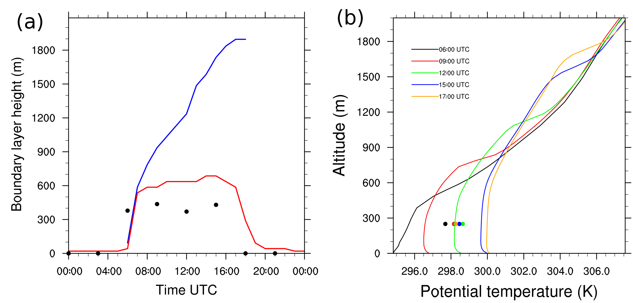
Figure 1(a) Boundary layer height diurnal evolution computed from the bulk-Richardson method (red), the tracer method (blue) and composite values of boundary layer height for the SOP-2 period (1 August 2006–15 August 2006) based on Gounou et al. (2012) (black dots). (b) Potential vertical temperature profiles at 06:00 (black), 10:00 (red), 14:00 (green) and 17:00 UTC (blue).
2.2 Chemical model setup
The chemical scheme ReLACS 3.0 (Reduced Lumped Atmospheric Chemical Scheme version 3.0) (Tulet et al., 2006) applied is a reduced version of the Caltech Atmospheric Chemistry Mechanism (CACM) (Griffin, 2002). This mechanism describes the reaction system of gaseous ozone precursors as well as of secondary organic aerosols (SOA) with 365 reactions involving 87 species.
For both simulations, the initial vertical profiles of the main primary chemical species are taken from airborne measurements made during the B235 flight of the AMMA campaign performed by the BAE-146 aircraft (Table 1). This particular flight gives access to measurements performed in the boundary layer over a tropical forest in the north of Benin (10.13∘ N, 2.69∘ E) during the early afternoon (Stone et al., 2010).
Biogenic emissions (Table 2) are taken from the MEGAN-MACC (Model of Emissions of Gases and Aerosols from Nature – Monitoring Atmospheric Composition and Climate) inventory (Sindelarova et al., 2014), except for NO, which is not available in this inventory. Biogenic NOx emissions from the GEIAv1 (Global Emission InitiAtive) inventory (Yienger and Levy, 1995) proved to be too low for the region studied in comparison to estimations based on airborne measurements during the AMMA campaign (Stewart et al., 2008; Delon et al., 2010). Therefore, a maximum value of 10 ng N m−2 s−1 was set for nitrogen oxide emissions from soils in the simulation.
Table 2Emission values for the biogenic and the anthropogenic cases, in kg m2 s−1. For NO, ISOP, BIOL and BIOH in the biogenic case, Gaussian shape emissions were set and only the maximum value is indicated here. Please see text for details.
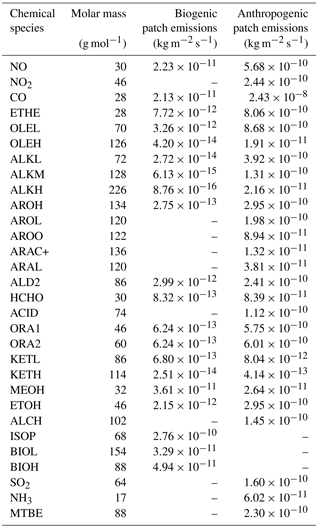
The emissions are constant in space and time except for NO, isoprene and monoterpenes, for which a Gaussian diurnal cycle is used. For biogenic NO, the maximum emission occurs at 13:00 UTC and the standard deviation of the Gaussian curve is equal to 3 h. These parameters are set in order to approximate the ground temperature, since Mamtimin et al. (2016) and Yienger and Levy (1995) noted that NO emissions from soils are closely linked to soil temperature. For isoprene and the sum of monoterpenes (represented as ISOP, BIOL and BIOH in the chemical scheme), the maximum occurs at 12:00 UTC and the standard deviation is equal to 2.5 h, chosen to fit the diurnal evolution of the solar radiation reaching the surface. This is in agreement with Guenther et al. (1991), who showed that isoprene emissions are thought to be null when photosynthetically active radiation (PAR) is equal to zero and maximum when the PAR exceeds the value of 1000 µmol m−2 s−1. For isoprene and monoterpenes, the maximum emission values were defined to ensure that an equal amount of chemical species is emitted over one day compared to the constant value provided by MEGAN-MACC.
The anthropogenic emissions are provided by a squared patch in the center of the domain. Its area is chosen as equal to half the domain area. However, the cyclic boundary conditions applied for these simulations tend to homogenize the chemical mixing ratios. This especially affects long-lived species in the boundary layer and leads to the deletion of the biogenic emission signature. The values of anthropogenic emissions are representative of Cotonou (Table 2) (Junker and Liousse, 2008).
In the following, the study focuses on isoprene for the biogenic case because it is the major biogenic VOC emitted into the atmosphere and influences ozone and secondary organic aerosol formation (Guenther et al., 2006). For the anthropogenic case, attention is given to the lumped C > 2 aldehydes (ALD2 in the chemical scheme) because they have both primary and secondary sources and their role is very important in the troposphere as they contribute to the production of radicals and are precursors of ozone (Williams et al., 1996).
2.3 Metrics
In order to study the competition between chemical reactivity and turbulent mixing, as well as inhomogeneity in chemical species mixing ratios, Schumann (1989) introduced two dimensionless numbers: the Damkhöler number and the segregation coefficient. The first corresponds to the ratio between the characteristic turbulence timescale τturb and the chemical reactivity timescale τchem. For a given compound A, the Damkhöler number Da is as follows:
where w* and h refer to the convective velocity and the boundary layer height (BLH), rA is the mixing ratio of A and ∑sinks(A) corresponds to the total chemical loss rate of A. The convective velocity is computed with g, the standard acceleration due to gravity, and θ, the potential temperature, according to the relation where stands for the buoyancy flux at the surface. Schumann (1989) distinguished different chemical regimes for the reaction between nitrogen oxide and ozone and found that the impact of turbulence on this reaction rate is highest for Da > 0.1. Later studies (Molemaker and Vilà-Guerau de Arellano, 1998; Vilà-Guerau de Arellano and Cuijpers, 2000; Vilà-Guerau de Arellano et al., 2005) have shown that the impacts of turbulence on atmospheric chemistry are expected to be maximum when Da≥1. Therefore, this value will be used in the following to discriminate slow and fast chemical reactions in the boundary layer. If Da<1, then the turbulent mixing is more efficient than the chemistry. If Da≃1, strong competition can be expected between dynamics and chemical reactivity. Finally, if Da>1, the chemical reactions occur faster than turbulent mixing.
The turbulent mixing causes fluctuations of chemical species mixing ratios in the LES domain, which can be quantified by the intensity of segregation. For a second-order reaction involving two species A and B with a reaction constant k: , the intensity of segregation IS(A,B) is defined as follows:
The lower case letters represent species mixing ratios at a grid point. The overline denotes a spatial average, and the prime a deviation from this average. If , then the two species are completely segregated and no reaction will take place between them. If , the compounds are perfectly mixed. A positive segregation coefficient means that the covariance between species is similar and thus the mean chemical reaction rate would be higher in comparison to perfect mixing. The segregation is calculated with mixing ratio anomalies related to spatial averages in numerical models. Ouwersloot et al. (2011) stated that these averages should correspond to the complete mixing volume in order to allow comparisons between models and measurements. In the following, the large-scale spatial average is calculated over the 10 km × 10 km model domain. An effective average reaction rate Re can be defined that includes the impact of turbulent mixing on chemical reactivity as follows:
Here, ke is the effective mean reaction constant. In the current LES experiments, chemical reaction rates are calculated with a focus on OH. OH radical reactivity ROH corresponds to the inverse of OH lifetime τOH and is defined as follows:
In Eq. (4), represents the reaction constant between OH and the i-th reactant, and χi corresponds to its concentration. As with the effective reaction constant Re, effective reactivity for the OH radical is defined by including the effect of turbulent mixing in Eq. (4) as follows:
ROH denotes the OH total reactivity calculated with averaged values. In order to obtain the relative deviation of the total OH reactivity from the reactivity computed with averaged mixing ratios, factorization is performed on Eq. (7), which results in the following:
From Eq. (9) the mean relative error, , found on total OH reactivity considering only averaged values is as follows:
The segregation intensity used to compute the mean error corresponds to the deviation from the averaged boundary layer values. This error on OH reactivity was not considered in previous numerical studies focused on identifying the missing part of OH reactivity. Indeed, using a box model or a single-column model like Mogensen et al. (2011), Whalley et al. (2011) or Whalley et al. (2016) leads to neglect of the turbulent motions that could affect the redistribution of chemical species within the atmospheric boundary layer. This may imply an underestimation or an overestimation of OH reactivity as a function of the sign of . If is positive or negative, then the effective OH reactivity is either higher or lower, respectively, than the OH reactivity ROH found by neglecting the turbulent motions. Due to the crucial aspect of the OH radical in the atmosphere, this could subsequently modify the lifetimes of gaseous OH reactants such as ozone and carbon monoxide.
2.4 Simulation assessment
2.4.1 Dynamics
The diurnal evolution of the boundary layer height is analyzed in Fig. 1a. It is diagnosed using two different methods. The first corresponds to a determination according to the bulk Richardson number method as presented in Zhang et al. (2014). The boundary layer height is defined as a threshold value for the bulk Richardson number Rib, computed at a given height with the virtual potential temperature θv and horizontal wind speeds uz and vz at this altitude and at the surface:
A clear diurnal cycle is observed, with the maximum height at 14:00 UTC and the minimum during nighttime (Fig. 1a, red line). This first diagnostic did not include the cloud layer on the boundary layer. Daytime BLH is consistent with observations from Cotonou in West Africa, studied by Gounou et al. (2012), who noticed daily variabilities ranging from 400 to 600 m (Fig. 1a, black dots). In Gounou et al. (2012), the boundary layer height is derived from radio soundings by comparing the virtual potential temperature at one level and the averaged value below.
The slight differences between the simulated BLH and observations reveal the same biases noticed in the one-dimensional simulation performed by Couvreux et al. (2014). This may be explained by uncertainties in the derivations of large-scale advection fields.
The second method determines the boundary layer height according to Vilà-Guerau de Arellano et al. (2005) by identifying the height at which a passive bottom-up scalar emitted at the surface is equal to 0.5 % of its surface value. Kim et al. (2012) mentioned that this definition could be valuable when studying boundary layer deepening due to clouds. This diagnostic captured the growth of the boundary layer height due to the development of cumulus clouds (Fig. 1a, blue line) and is used to mark the BLH in the following. The tracer used for this diagnostic was emitted only during the period of interest, from 06:00 to 18:00 UTC.
The range of simulated virtual potential temperature (Fig. 1b) overestimates the AMMA observations in Cotonou of Gounou et al. (2012) in the lowest 500 m, as shown by Couvreux et al. (2014). At 06:00 UTC, the model has a cold bias of −2 K turning throughout the simulation to a simulated potential temperature overestimated by +2 K at the end of the simulation. Both the dry and cloudy layers are identified by two inflections on the vertical profiles of the virtual potential temperature (Fig. 1b). The first inflection increases from 400 m at 06:00 UTC to 600 m at 17:00 UTC, corresponding to a thin inversion zone between the well-mixed dry layer and the cloudy layer above it. The second inflection defines the top of the boundary layer ranging from 500 m at 06:00 UTC to 1600 m at 17:00 UTC.
The southern part of West Africa is a region characterized by high diurnal variability in cloud occurrence. Low-level stratus clouds form during the night and persist in the morning; these stratus then break up during the afternoon into cumulus clouds (Schrage et al., 2007). This feature is simulated in this work as low-level stratus clouds that occupy a large fraction of the simulated domain in the morning (Fig. 2a and c). In the afternoon, the cloud deck breaks up and less uniform but higher cumulus clouds are simulated (Fig. 2b and d).
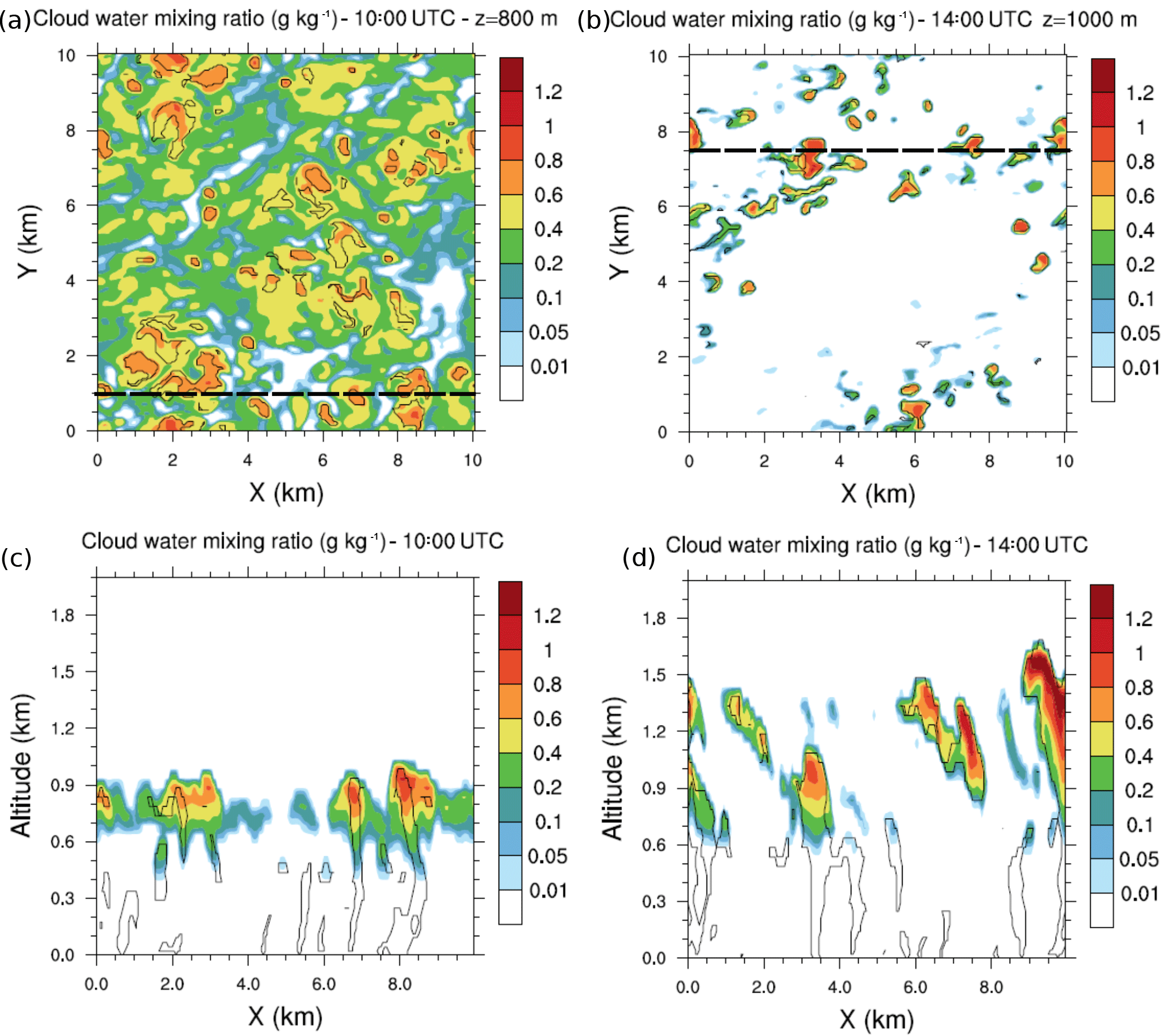
Figure 2(a) Cloud water mixing ratio horizontal cross sections at 10:00 UTC and 800 m height and (b) at 14:00 UTC and 1000 m height. Black dashed lines represent the vertical cross sections at (c) 10:00 UTC and y=1 km and at (d) 14:00 UTC and y=7.5 km. Black isolines denote thermals identified by the conditional sampling method.
Throughout the growth of the boundary layer, dry thermals develop capped by the temperature inversion zone. Some thermals penetrate this inversion (Fig. 2) and cloud formation occurs at the upper part of the updrafts. The vertical profiles of the fraction area (Fig. 3) occupied by thermals exhibit a local maximum at the height corresponding to the separation between the two layers. This altitude is variable through the simulation but tends to stabilize between 500 and 600 m in the early afternoon and is associated with a preferential detrainment zone. The peaks observed at the surface and at the top of the cloudy layer correspond to two other local maxima. Due to the deepening of the boundary layer, the top of the cloudy layer increases throughout the simulation (Figs. 2 and 3). Simulated convective velocity w* ranges from 1 cm s−1 in the morning to 1 m s−1 at midday, and the turbulence characteristic timescale τturb from 6 h in the morning to 20 min at midday.
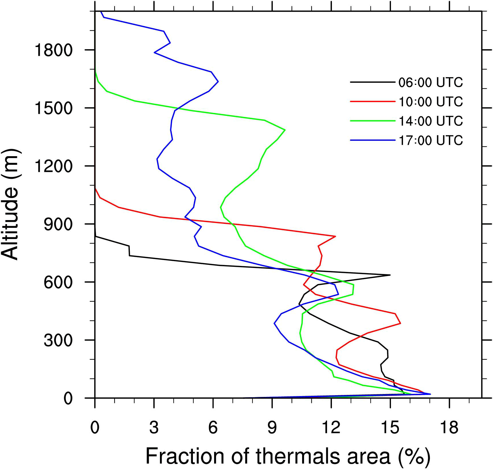
Figure 3Vertical profiles of the fraction occupied by thermals at 06:00 (black), 10:00 (red), 14:00 (green) and 17:00 UTC (blue).
2.4.2 Atmospheric chemistry
Typical diurnal cycles are obtained for isoprene in the biogenic case and for OH in the biogenic and anthropogenic cases in which both compounds exhibit maximum mixing ratios around midday (Fig. 4). For the biogenic case, the simulated isoprene mixing ratios averaged from the surface to 600 m reach a maximum close to 1 ppbv (Fig. 4a) at noon, when isoprene emissions are highest. This is in the same range as the AMMA measurement studied by Saxton et al. (2007), who found a maximum of 1.5 ppbv on the composite diurnal cycle of isoprene at midday. In our study, the ozone mixing ratios did not exhibit strong variability throughout the day. The simulated values around 18 ppbv were lower than the observations recorded over forested areas (Table 3), ranging from 22 to 30 ppbv. The NOx mixing ratios were close to 0.2 ppbv on average around midday (Fig. 4b) and are in agreement with AMMA measurements where a mean value of 0.1 ppbv of NOx was observed. Simulated OH mixing ratios varied between 0 and 0.18 pptv (Fig. 4a), within the observational range of 0.05 to 0.15 pptv during the AMMA campaign (Table 3). The biogenic environment is characteristic of a limited NOx regime.
Commane et al. (2010)Reeves et al. (2010)Borbon et al. (2012)Murphy et al. (2010)Ferreira et al. (2010)Murphy et al. (2010)Saxton et al. (2007)Commane et al. (2010)Reeves et al. (2010)Delon et al. (2010)Ancellet et al. (2009)Thouret et al. (2009)Murphy et al. (2010)Ancellet et al. (2009)Commane et al. (2010)Table 3Measurements collected during the AMMA campaign over forested areas (upper part) and over cities (lower part). The last column corresponds to the concerned period.
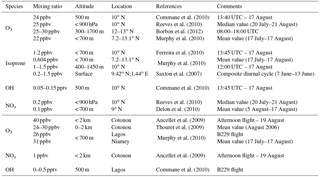
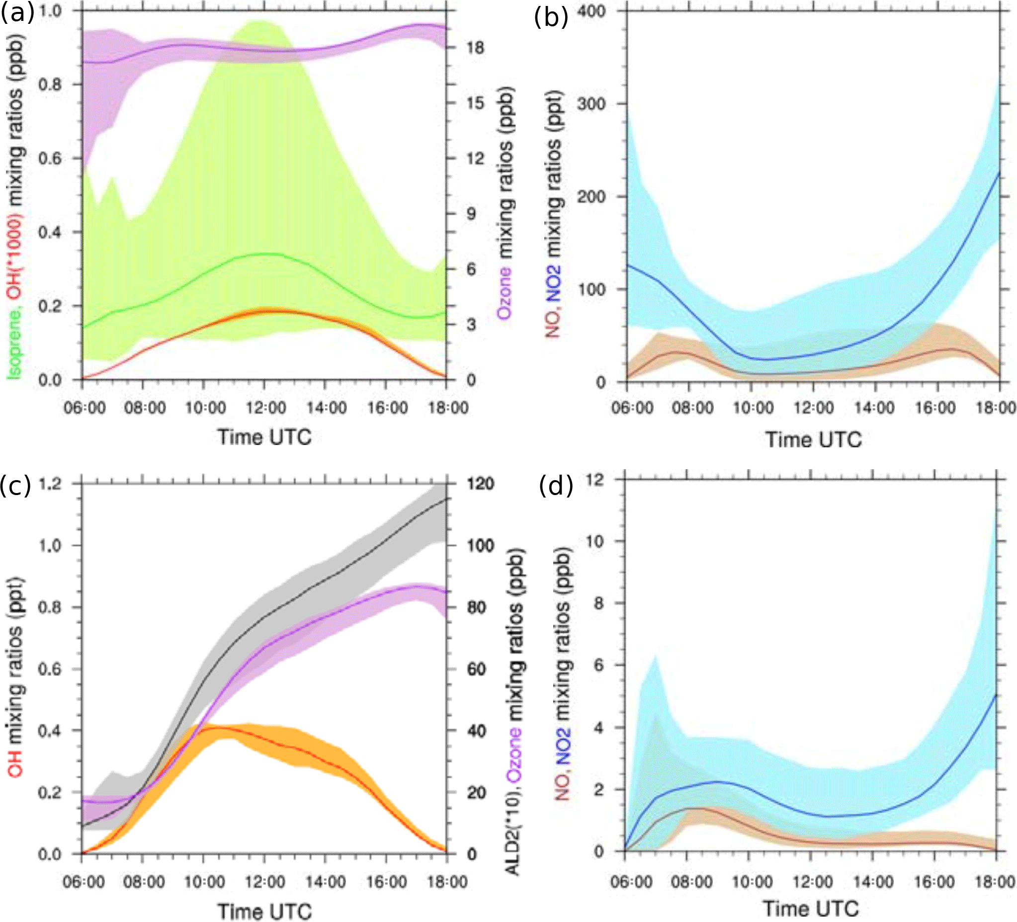
Figure 4(a–b) LES-simulated diurnal cycles for isoprene (green), OH (red), ozone (purple), NO (brown), NO2 (blue), (c–d) ALD2 (grey), OH (red), ozone (purple), NO (brown) and NO2 (blue). Panels (a–b) correspond to the biogenic environment, (c–d) to the anthropogenic environment. The shaded areas denote the minimum and maximum of mean vertical profiles between the surface and 600 m height, and the colored lines correspond to the averages of these profiles.
The chemical regime induced by the anthropogenic emissions is contrasted with the previous biogenic case (Fig. 4c and d), including NOx emissions nearly 40 times higher at 13:00 UTC. The averaged NOx mixing ratio was 1.5 ppbv at midday (Fig. 4d), which is similar to the averaged value of 1 ppbv measured during a flight over Cotonou during the AMMA campaign (Table 3). The increase in NO and NO2 led to considerable oxidant formations. OH mixing ratios varied between 0 and 0.40 pptv in the simulation, in agreement with the AMMA measurements ranging from 0 to 0.50 pptv over Lagos (Table 3). Ozone was produced throughout the simulation but did not exhibit strong spatial variabilities. Its mixing ratios varied from 17 ppbv in the morning to 82 ppbv in late afternoon. This was higher than the observations recorded over several cities in West Africa, varying between 26 and 40 ppbv (Table 3). ALD2 increased continuously during this case through chemical production and emissions (Table 2). Its mixing ratios ranged from less than 1 ppbv in the morning to 11 ppbv at the end of the simulation. Unfortunately, no aldehyde observations, except formaldehyde, were available from the AMMA experiment despite the use of a PTR-MS due to interferences during the measurements for identified as acetaldehyde (Murphy et al., 2010).
A minimum of NOx was found around 12:00 UTC for both cases and can be explained by two factors. The first is dynamical and is linked to the boundary layer. In the middle of the simulation, the boundary layer growth was maximal and induced dilution in a larger mixing volume. The second factor was chemical because at that instant, NO was efficiently converted into NO2. However, NO2 chemical transformations in a reservoir such as HNO3, HNO4 or PANs are net sinks for NO2. The chemical balance between reservoir species and NO2 represented 2.12 % of the net destruction of NO2 averaged over the domain at 20 m and 12:00 UTC for the biogenic case, and 34.2 % for the anthropogenic case. For both cases, the main reservoirs of NO2 were PAN1 and PAN2. Therefore, less NO2 was available for conversion into NO, which explains the low NO mixing ratios at midday (Fig. 4b and d).
3.1 Impact of turbulent mixing on the OH reactions
3.1.1 Vertical transport and Damkhöler numbers
Isoprene is highly reactive, especially towards OH, and is rapidly consumed in the boundary layer linked to its chemical lifetime τch, approximately equal to 30 min in the biogenic case. The Damkhöler number of isoprene is close to 1 (Table 4), indicating that the isoprene chemical lifetime is comparable with the timescale of turbulent mixing. This implies that chemical reactions and turbulent mixing are competing processes for this compound. Isoprene is both transported and consumed inside the thermals and exhibits vertical and horizontal gradients (Fig. 5a). The average profiles of isoprene decrease with altitude (Fig. 5a). The lower mixing ratios in the updraft-free region (dashed line) are close to the domain-averaged values due to domain coverage by thermals (Fig. 3). Updraft regions contain higher isoprene mixing ratios with significant anomalies over the whole boundary layer, although these ratios decrease with rising altitude.
Table 4Simulated Damkhöler number of chemical species averaged from the surface to 0.6 km at 12:00 UTC for the two cases calculated with τturb ≈ 20 min.
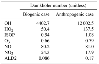

Figure 5(a) Isoprene (ppb) and (b) OH radical (ppt) mixing ratios for the biogenic case at 12:00 UTC. (c) ALD2 (ppb) and (d) OH radical (ppt) mixing ratios for the anthropogenic case at the same time. For each figure, the left part consists of a vertical cross section at the middle of the domain (y=5 km). Black isolines denote thermals identified by the conditional sampling method. In the right part of each panel, the shaded areas denote twice the standard deviation at a given altitude and the line represents the horizontal average over the domain. The dashed line corresponds to the average in the environment and the dotted lines inside thermals.
For the biogenic case, OH has a very short chemical lifetime of the order of 0.2 s. The OH radical rapidly reaches steady state and is relatively undisturbed by the turbulent mixing, as evidenced by its large Damkhöler number (Table 4). Therefore, OH mixing ratios (Fig. 5b) have almost homogeneous values below 600 m with no distinction between thermals and their environment. Average OH profiles (Fig. 5b) show no strong variability below 600 m in the boundary layer. Above this height, the thermals have lower OH concentrations on average with relatively small differences. The differences between thermals and their surroundings are more pronounced in the cloudy layer because clouds arise from air parcels transported by thermals and characterized by lower OH mixing ratios than the rest of the domain. Since OH is almost constant over the boundary layer, the highest reaction rate for the oxidation of isoprene by OH (kOH+ISOP[ISOP][OH]) is located where the isoprene mixing ratios are the highest. This implies that both the surface and air lifted by thermals are preferential reaction zones in the boundary layer.
For the anthropogenic simulation, the reaction rate of ALD2 with OH is lower than the reaction rate of OH with isoprene. Its calculated Damkhöler number (≈ 0.17) indicates that turbulent mixing dominates over chemical reactions (Table 4). Consequently, ALD2 is efficiently transported by updrafts (Fig. 5c). The contrast between concentrated air parcels lifted upwards by thermals and relatively diluted air outside is illustrated by the large differences in the ALD2 average profile in thermals and in the environment (Fig. 5c). As with isoprene in the biogenic case, the two-layer structure presented above is present on the vertical profiles. It results from the mixing in the sub-cloud layer and from the mixing within clouds.
OH mixing ratios are nearly twice as high in the anthropogenic environment as in the biogenic case, inducing a more reactive atmosphere and a shorter chemical lifetime for species whose OH is the main sink in the boundary layer. OH has a very short chemical lifetime of 0.07 s in this simulation, which represents a large Damkhöler number close to 12 000. OH mixing ratios are maximal in thermals (Fig. 5d) due to the transport of OH precursors, such as NOx, and fast steady state. Conversely, lower mixing ratios in average OH profiles (Fig. 5d) correspond to regions without updrafts, leading to strong OH anomalies within updrafts from the surface to the top of clouds.
3.1.2 Vertical profile of segregation intensity
Negative values of segregation coefficients up to −30 % are calculated at the top of the cloudy boundary layer from 10:00 to 17:00 UTC which means that OH and isoprene are partly segregated in this frontier zone. In other words, the hypothesis of a well-mixed atmosphere would lead to a 30 % overestimation of the reaction rate at the frontier between the boundary layer and the free troposphere. The negative segregation (Eq. 2) means the anomalies of isoprene and OH have opposite signs, as shown in Fig. 5a. This is due to lower OH mixing ratios in thermals than in the environment (Fig. 5b). These results are consistent with the previous studies of Li et al. (2016), Kim et al. (2016) and Ouwersloot et al. (2011) (see Discussion).
In the biogenic case, isoprene anomalies in thermals are considerable from the surface (+0.48 ppbv on average at midday) to the top of the boundary layer (+0.1 ppbv on average at midday) and are thought to be always positive as OH is uniformly emitted at the ground (Fig. 5a). On the contrary, OH mixing ratios are almost constant in the boundary layer at 12:00 UTC (Fig. 5b), so the magnitude of OH anomalies are expected to be low (−0.03 pptv on average at midday at the top of the boundary layer). Besides, due to its very short chemical lifetime, OH quickly reaches equilibrium with its surroundings, implying that its fluctuations are mostly due to thermals transporting air originating from different chemical environments. Thus, isoprene anomalies are thought to be the major driver of the magnitude of segregation over the boundary layer, whereas changes in OH anomalies are related to changes in the segregation sign.
Positive values around +5 % are calculated at 700 m starting from 14:00 to 18:00 UTC (Fig. 6a). The intensity of segregation becomes positive due to positive anomalies of both compounds. Due to a decrease in isoprene emissions in the afternoon, OH destruction slows down, especially inside thermals. They are still active in transporting enough NO to react with HO2 to produce OH, inducing higher OH mixing ratios inside updrafts than in the surroundings (+0.02 pptv on average at 16:00 UTC).
Before 09:00 UTC near the surface, the segregation coefficient in the anthropogenic simulation between OH and ALD2 is negative up to −8 % in the lower 200 m (Fig. 6b), due to the anthropogenic emission patch. As chemical equilibrium is not yet reached, more of the OH radical is destroyed through its reaction with recently emitted compounds than that which is produced (not shown). This means that OH is less concentrated inside updrafts at that moment so its anomalies are negative near the surface. Simultaneously, positive segregations develop at the top of the boundary layer from 07:00 to 12:30 UTC with a maximum of 16 % at 10:00 UTC and from 15:30 to 17:30 UTC. The positive segregation is related to the concomitant transport of ALD2 and precursors of OH by thermals. Moreover, the high segregation values correspond to the presence of clouds between 0.6 and 0.9 km (Fig. 2c), simultaneous with a high cloud fraction over the domain (>0.6) (Fig. 6b). This specific point is discussed in the Discussion. As ALD2 is emitted at the surface, its anomalies are high and positive inside updrafts. For example, at midday, anomalies are +0.5 ppbv on average at the surface and nearly +4 ppbv at the top of the boundary layer. However, in this case, OH anomalies are more difficult to predict due to the spatial heterogeneities of chemical emissions. Local changes in OH production and destruction explain the changes in the segregation sign throughout the simulation. Except for positive segregation simulated between 500 and 1400 m from 11:30 to 16:00 UTC with values ranging from 2 to 4 %, ALD2 and OH can be considered well-mixed in the central part of the boundary layer. The ALD2 oxidation reaction by OH is accelerated up to 16 % at the top of the cloudy layer from the morning to the early afternoon compared to a perfect mixing assumption.
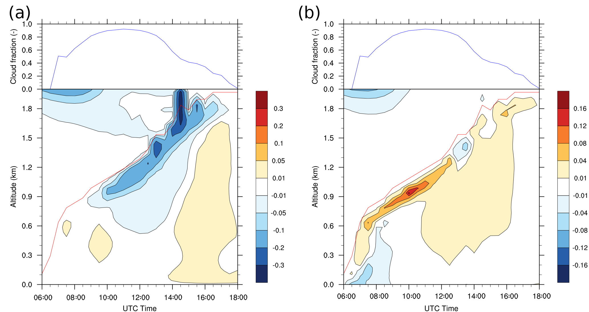
Figure 6(a) Diurnal evolution of the segregation coefficient for isoprene and OH in the biogenic case and (b) for ALD2 and OH in the anthropogenic case. The red line represents the boundary layer height as determined by the tracer approach. The diurnal evolution of cloud fraction (blue line) is added above each panel.
Regarding the two simulations, the segregation has both spatial and temporal variations. The maximum values of the segregation coefficient are calculated near the top of the boundary layer. Below and during daytime, the considered species are well-mixed for both cases. This means that in the biogenic environment, the highest decrease induced by the thermals of isoprene + OH reaction is located near the top of the boundary layer. It also implies that in the anthropogenic environment, the highest increase induced by the thermals of isoprene and ALD2 + OH reaction is also located near the top of the boundary layer.
3.2 OH budget and reactivity in a convective boundary layer
The previous part emphasized the nonuniform mixing between isoprene and OH for the biogenic case and between OH and ALD2 for the urban case, and the modification of the reaction rates between these species. However, this feature must be taken into account for every OH reactant in order to obtain the full picture of total OH reactivity and gain insight into how the Meso-NH model computes the OH budget in different chemical regimes.
3.2.1 OH budget in thermals versus surroundings
In order to identify and quantify the major OH sources and sinks in the boundary layer, the instantaneous chemical budget of OH at 20 m above ground level is investigated at 12:00 UTC for both environments (Fig. 7). This height is the first level in the model, and computing the chemical budget at this height leads to uncertainties due to subgrid-scale mixing and chemistry (Vinuesa and Vilà-Guerau de Arellano, 2005). However, it makes it possible to compare the model results with the measurements in the literature.
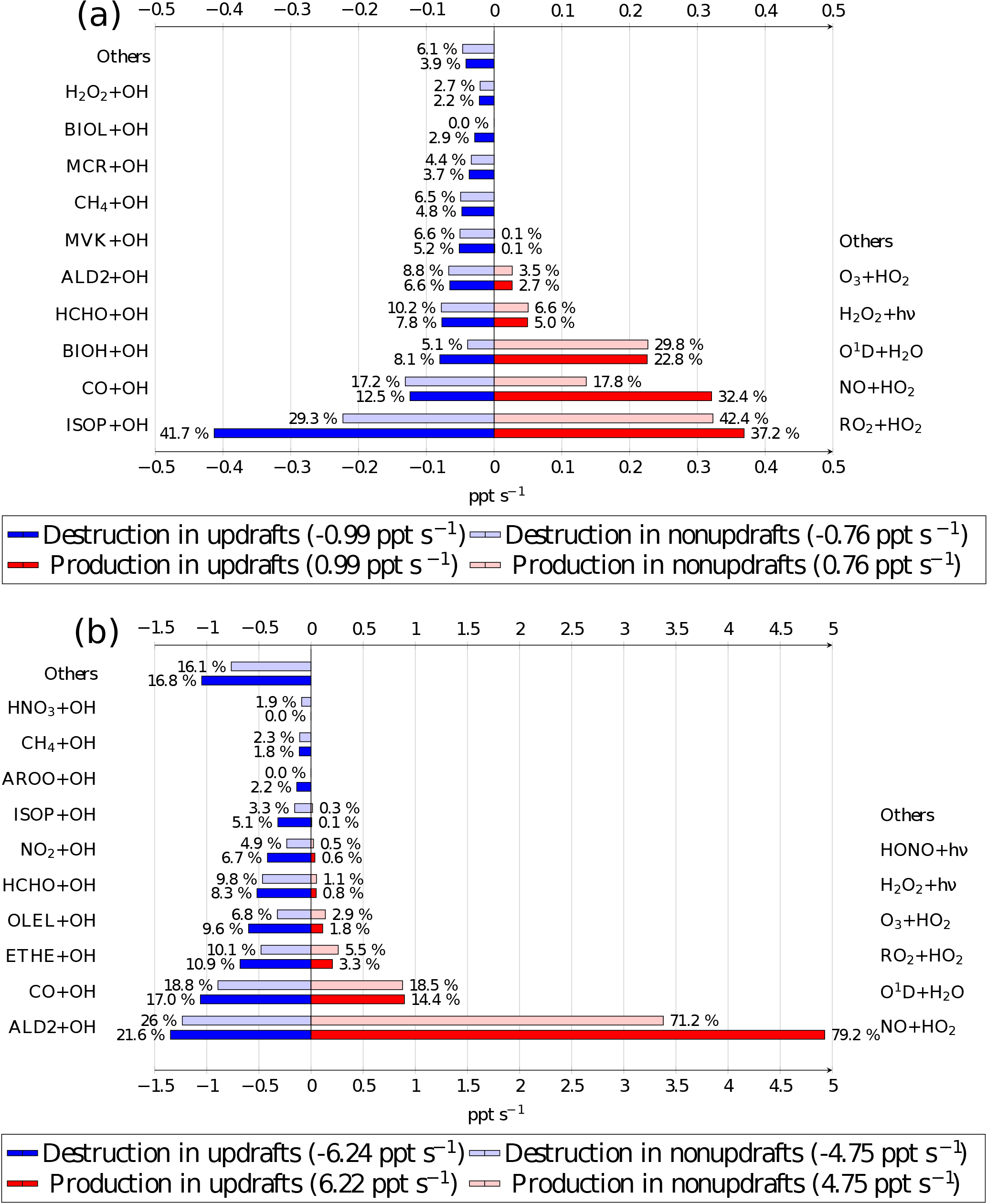
Figure 7OH radical chemical budget at 12:00 UTC averaged at 20 m for the biogenic (a) and the anthropogenic case (b). Source terms are in red for updrafts and pale red for nonupdrafts. Destruction terms are in blue for updrafts and pale blue for nonupdrafts. The bar lengths determine the absolute values, and the relative contributions for destruction and production are given by the percentage near each bar. Numbers between parentheses in the legend box are the OH production and destruction rates in updrafts and in nonupdrafts. Chemical names correspond to the names given in the ReLACS 3 mechanism.
The budget distinguishes between updraft and updraft-free columns. Percentages are related to the fraction of the overall production and destruction within or outside thermals. In the biogenic case (Fig. 7a), the OH budget is dominated by its destruction by isoprene oxidation (41.7 % of the total loss in updrafts and 29.3 % of the total loss in the rest of the domain) and its production by the reaction of peroxy radicals with HO2 (37.2 % of its total source in updrafts and 42.4 % of the total source in nonupdrafts) and NO reaction with HO2 (32.4 % of the total source in updrafts and 17.8 % of its total source in the rest of the domain). In this case, the peroxy radicals are mainly formed by the oxidation of isoprene and its degradation products. The absolute value of OH reactivity is higher in thermals than in the rest of the domain.
The OH budget for the anthropogenic case (Fig. 7b) shows that the chemical reactivity is higher inside thermals at the surface compared to the rest of the domain. The budget is largely dominated by the production of OH by NO + HO2 (79.2 % of its total source in updrafts and 71.2 % of the total source in nonupdrafts) and by O1D + H2O (14.4 % of the total source in updrafts and 18.5 % of its total source in the rest of the domain). Over the whole domain, ALD2 + OH (21.6 % of the total loss in updrafts and 26.0 % of the total loss in the rest of the domain) is the most important sink at the surface, followed closely by the oxidation of carbon monoxide (17 % of the destruction of OH in thermals and 18.8 % in nonupdrafts).
The chemical budget at 1200 m (Fig. 8), namely at the top of the boundary layer, allows the investigation of chemical reactions inside the ascending air parcel lifted by thermals and its comparison with its surroundings. For the biogenic case, the major OH reactants in the thermals have a chemical lifetime greater than the turbulence timescale. At this altitude, only species whose Damkhöler numbers are lower than 1 are present in sufficient amounts to react with the OH radical. For example, carbon monoxide (26.2 % of total OH destruction in thermals and 36.6 % in the surroundings) is the major sink, but also methane (11.8 % of total OH loss in updrafts and 18.4 % in the environment). Chemical compounds with a secondary source like formaldehyde and C > 2 aldehydes (ALD2) are other important sinks at 1200 m. Isoprene, the major OH reactant close to the surface, is present only in thermals at this altitude due to its reaction with OH in the ascending air parcel and consumes 11.8 % of OH in thermals. OH production by NO + HO2 reaction is null inside updrafts and low in the nonupdraft area (3.2 % of the total OH production) due to NO destruction in updrafts. The reaction between hydroxyl radicals RO2, secondary products, with HO2 is a major OH source in thermals (49.7 % of total production) but also in the surroundings (36.1 % of OH production in updraft-free region). Production of OH by O1D + H2O or H2O2 photolysis are similar in magnitude in thermals and in the nonthermal areas. The production and destruction terms are higher in the thermals compared to these terms in nonupdrafts due to higher concentrations of OH reactants inside the thermals, but lower than at 20 m.

Regarding the anthropogenic case, species whose lifetimes are higher than the turbulence timescale are major OH reactants at 1200 m. Carbon monoxide contributes 22 % of the OH destruction in thermals and 34.3 % in the rest of the domain. As with the biogenic case, chemical compounds with a secondary source are important OH sinks like formaldehyde (11.1 % in thermals and 11.0 % in updraft-free regions) and ALD2 (26.4 % of total OH destruction in updrafts and 11.8 % in the surroundings), corresponding to the major OH destruction term at the top of the boundary layer. The OH production terms in the anthropogenic case are similar in thermals compared to the surface, with a high contribution of NO + HO2 reaction (66.9 % of total OH production), followed by O1D + H2O reaction (15.3 %) and RO2 + HO2 (10.6 %). In the rest of the domain, NO + HO2 contribution drops to 12.7 % while O1D + H2O (49.4 %) and RO2 + HO2 (23.4 %) are major production terms.
The differences between the OH reactivity at the surface and the top of the boundary layer are mainly driven by the changes in chemical mixing ratios of precursors caused by chemical reactions and consequently by their Damkhöler number, and by the secondary products formed inside the thermals.
3.2.2 OH reactivity in the convective boundary layer
The OH reactivity for the biogenic case (Eq. 4) at 20 m is maximum around midday and is equal to 6.0, 4.25 and 4.55 s−1 respectively in updrafts, in nonupdrafts and averaged over the domain (Fig. 9a). This feature is linked to the photochemical maximum activity at noon, and the diurnal cycle of emissions amplifies this phenomenon. At that time and near the surface, many chemical compounds are available to react with OH, which leads to a high value of reactivity. The values in updrafts are higher than outside due to higher reactant mixing ratios inside thermals (Fig. 5a). The arithmetical difference between updrafts and nonupdrafts reaches a maximum at 12:00 UTC and is about 1.75 s−1. However, as the thermals occupy less than 15 % of the domain (Fig. 3), the evolution of the domain-averaged OH reactivity is very similar to that linked to updraft-free regions.
The diurnal cycle of OH total reactivity with a maximum around midday in a biogenic environment is well documented in the literature on observations of OH reactivity for a Mediterranean forest (Zannoni et al., 2016), for temperate forests (Sinha et al., 2008; Ramasamy et al., 2016) and for tropical forests (Nölscher et al., 2016; Williams et al., 2016). The values of OH reactivity in or outside thermals in the present study are the lower bounds of measurements taken over forests and gathered in Yang et al. (2016), between 1 and 76 s−1.
The mean relative error made on OH reactivity is calculated by Eq. (10) (Fig. 10). This diagnostic includes the segregation, computed relative to the boundary layer averaged values, between OH and every one of its reactants in the chemical scheme. It is negative throughout the simulation, increases during the morning and is maximal in the early afternoon with a peak at −9 % at 14:30 UTC. In other words, neglecting the segregation of reactive species by turbulent mixing in the boundary layer would lead to overestimating OH reactivity by 9 % at most in an environment dominated by biogenic emissions.
For the anthropogenic case, total OH reactivity (Eq. 4) in thermals and in the rest of the domain does not present a clear diurnal cycle (Fig. 9b). From the 08:00 UTC value of 11.6 s−1, the domain-averaged OH reactivity fluctuates but tends to increase to 14.2 s−1 at 16:00 UTC. The evolution of the OH reactivity in thermals is similar and ranges from 14.8 s−1 at 08:00 UTC to 17.7 s−1 at 16:00 UTC. For the same period, the values in updraft-free domains vary between 11 and 13.5 s−1. The consequence of higher OH reactant mixing ratios in the boundary layer (Fig. 4c and d), is higher OH reactivity in this case compared to the biogenic simulation.
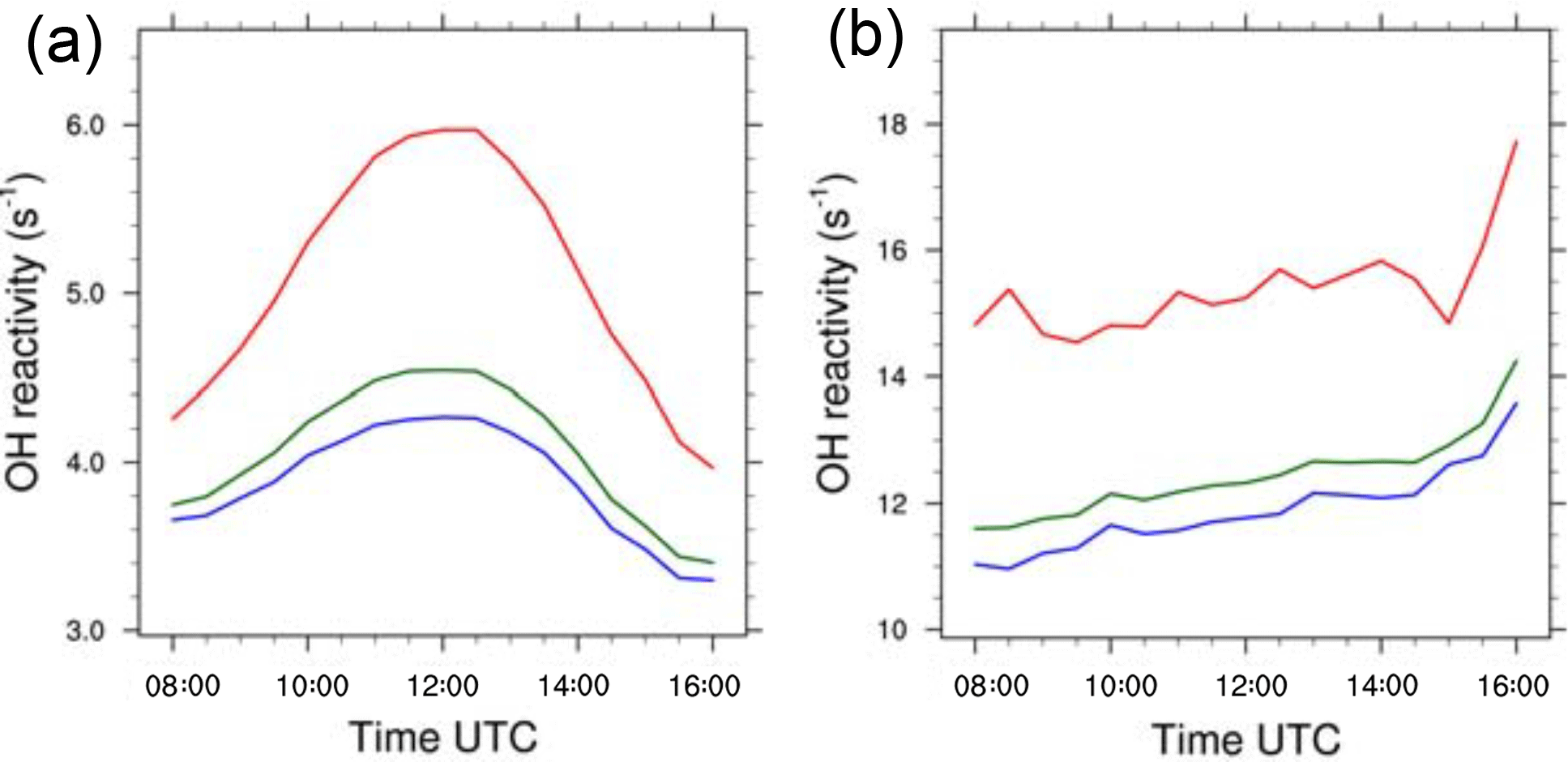
Figure 9(a) OH reactivity (s−1) in thermals (red), domain averaged (green) and in a nonthermal region (blue) averaged at z=20 m for the biogenic and (b) the anthropogenic case.
The mean relative error of the OH reactivity (Eq. 10) is generally positive throughout the simulation (Fig. 10). It ranges between 0 and 4 % from 09:00 to 16:00 UTC with a maximum value of 4.5 % at 13:30 UTC. In this case, the turbulent mixing induces a moderate increase up to 4.5 % of the total OH reactivity for two reasons. The segregation effect is limited to the last 200 m of the boundary layer. Thus averaging on the whole boundary layer cancels the extreme values. Moreover, chemicals have either negative or positive segregation towards OH that may compensate or increase the positive values simulated for ALD2 and OH (Fig. 6b).
In both cases, the occurrence and development of clouds (Fig. 6, upper panel) is concomitant with linear increases in the error made on the OH reactivity while neglecting the impact of turbulence (Fig. 10). The diurnal cycle of in each case is correlated to the development of the convective boundary layer. Firstly, a rapid change occurs during the first hours of the simulations, characterized by the occurrence of thermals and an increase in chemical emissions for the biogenic environment. Then, is relatively stable from the end of the morning to the middle of the afternoon, with a maximum value computed around 14:00 UTC, corresponding to the maximum turbulent activity in the convective boundary layer.
The redistribution of chemical species by the boundary layer turbulence induces a different mean reaction rate between compounds when compared to a situation in which chemical species would be perfectly mixed (Krol et al., 2000; Ouwersloot et al., 2011; Kim et al., 2012, 2016; Li et al., 2016, 2017 among others). The perfectly mixed assumption used in regional- and large-scale atmospheric models leads to errors in the mean reaction rates between species as the turbulent mixing occurs at scales smaller than the grid length (Vinuesa and Vilà-Guerau de Arellano, 2005). This implies that the OH total reactivity has been calculated inaccurately, in turn leading to a modification in the lifetimes of the OH reactants such as ozone and carbon monoxide.
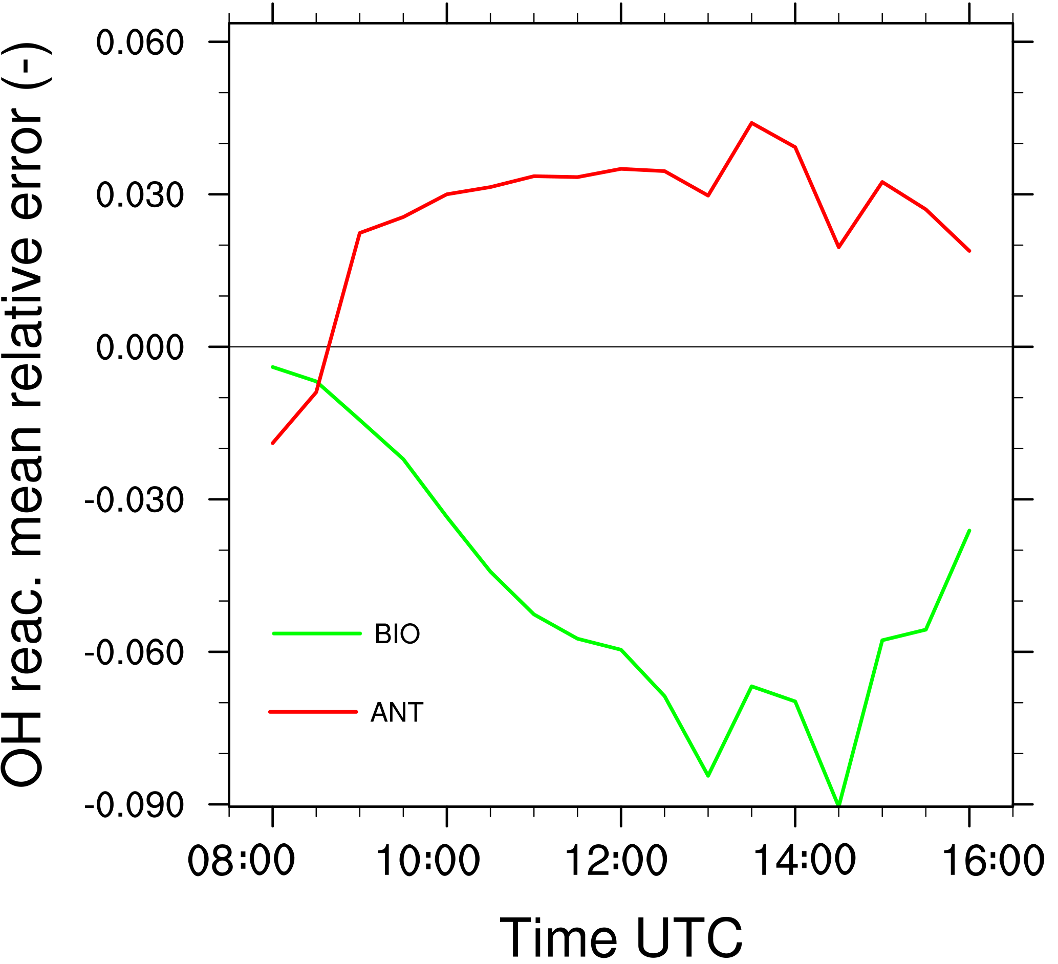
Figure 10Mean relative error made on the OH reactivity by neglecting turbulent motions for the biogenic case (green) and the anthropogenic case (red).
In a biogenic environment characterized by low NOx conditions, Kim et al. (2016) found negative segregation between isoprene and OH varying between −3 % near the surface and −10 % in the cloud layer due to increasing OH mixing ratios in thermals with altitude. That implied positive isoprene anomalies and negative ones for OH in the frontier region between the boundary layer and the free troposphere. These features are reproduced in our biogenic simulation although our segregation values are higher in the cloud layer (Fig. 6) due to sharper gradients of OH mixing ratios at the top of the cloudy layer.
Using a simple chemistry scheme of 19 reactions representing the basic reactions of the O3–NOx–VOC–HOx system, Ouwersloot et al. (2011) found an almost constant value of −7 % for the segregation between OH and isoprene in the boundary layer over the Amazonian forest. This was the result of positive isoprene anomalies due to transport by thermals and negative OH anomalies due to consumption therein. Negative segregation ranging from −2 to −5 % inside the convective boundary layer was simulated by Li et al. (2016) and Kim et al. (2016). In the biogenic case in this study, the negative segregation of a few percent in the middle of the boundary layer is reproduced. As in this case, higher segregation values were simulated with altitude in Kim et al. (2016), especially in the cloudy layer. However, segregation computed in the cloudy layer in Kim et al. (2016) was equal to −0.1, a value lower than that computed in the biogenic case of the present study. The discrepancies in this study and Kim et al. (2016) are likely due to the vertical OH profiles. In the study by Kim et al. (2016), OH concentrations increased linearly with altitude. This implies lower OH covariances for ascending air parcels and thus lower segregation values (Eq. 2). On the contrary, in the present study, OH is relatively homogeneous in the boundary layer and a strong gradient is present only at the top of the boundary layer. This induces high covariances for OH concentrations inside air transported by thermals at the top of the boundary layer, implying higher segregation values. As segregation computed by Li et al. (2016) is not available above 1000 m height, a direct comparison with results regarding the cloudy layer is not possible with the results from the biogenic case. The positive values of segregation simulated in the afternoon (Fig. 6a) in the biogenic case are not reproduced in other studies and might be the result of efficient OH recycling in ReLACS 3.0, initiated in particular inside the thermals due to peroxy radicals formed by isoprene oxidation. Indeed, this recycling is either absent or indirect in previous works like in the mechanism used by Kim et al. (2016) that produces only HO2 from peroxy radicals, which may explain the discrepancies in OH covariances. Furthermore, Ouwersloot et al. (2011) and Kim et al. (2016) investigated the sensitivity of segregation to NOx. It was found that different NOx levels imply differences in the segregation of OH and other compounds as they contribute to OH production.
Kim et al. (2012) used LES to study the OH budget in a biogenic environment averaged over the domain and over time from 13:30 to 14:30 LT with a chemical scheme adapted from MOZART v2.2. For a low NOx case with ozone mixing ratios close to 64 ppbv, they found that OH production was mostly influenced by four predominant reactions (including O1D + H2O, HO2 + O3, H2O2 photolysis and HO2 + NO). These production terms are present in the biogenic case of the present study. However, Kim et al. (2012) did not take into account recycling by peroxy radicals as the latter formed only HO2 in the chemical scheme they used. Moreover, they found that OH loss by reaction with isoprene was dominant near the surface, followed by reactions with CO and formaldehyde, as in the present study. The contribution of BVOC species to OH reactivity was simulated by Li et al. (2016) for three distinct biogenic cases of the DISCOVER-AQ (Deriving Information on Surface Conditions from Column and Vertically Resolved Observations Relevant to Air Quality) campaign. The production terms of OH were not available but it was found that isoprene was a dominant sink for OH; about 25–30 % of the OH reactivity was linked to BVOC reactions at 0.3 km during midday. This contribution is comparable to the percentage calculated for isoprene in the OH destruction in thermals (41.7 %) or in an updraft-free area (29.3 %). The contribution of formaldehyde was comparable to isoprene at that height, with HCHO mixing ratios ranging from 2 to 4.5 ppbv at the surface. The higher formaldehyde contribution of Li et al. (2016) is the result of higher concentrations than in the current work.
Yang et al. (2016) found that in forest areas the OH budget was largely dominated by isoprene and its oxidation products. For example, Zannoni et al. (2016) measured OH reactivity and the concentration of biogenic compounds over a Mediterranean forest. They found that isoprene was the dominant sink for OH and contributed up to 74 % of total OH reactivity during daytime due to its high reactivity towards OH and its high concentration over the forested area. Isoprene predominance in OH loss was reproduced in the OH budget of the biogenic environment of the present study, and for carbon monoxide. The formaldehyde mixing ratios were close to 2 ppbv, which explains that this is not a major sink like isoprene, but remains important for OH loss through the reaction OH + HCHO. OH production in the biogenic case was similar to Kim et al. (2012), as almost the same production terms are present. However, overall production was dominated by the reaction of peroxy radicals with HO2, and the ozone mixing ratios of 18 ppbv decrease the importance of O1D + H2O source for OH.
However, the mechanism used to represent atmospheric chemistry in our simulation has fast OH cycling due to the reaction of peroxy radicals RO2 with HO2. This reaction yield in OH is greater than in the laboratory studies (Hasson et al., 2004; Jenkin et al., 2007; Groß et al., 2014; Winiberg et al., 2016), implying an overestimation of OH mixing ratios, especially in the biogenic case where RO2 values are high. As the hydroxyl radical is recycled through the isoprene oxidation products, it tends to reduce the impact of isoprene chemistry on OH mixing ratios and thus influences the low segregation simulated in the core of the boundary layer. This is similar to a case considered by Stone et al. (2011) where an ISOPO2 + HO2→ ISOPOOH + 3 OH recycling mechanism was proposed to increase the simulated OH concentrations and provided the best agreement with OH observations. This reaction implied that isoprene has no net impact on OH concentrations. This conclusion was also reached by Kubistin et al. (2010) who found better agreement between simulated and measured HOx concentrations by ignoring isoprene chemistry. As the chemistry of isoprene is not well understood, the results obtained in our work are subject to these uncertainties.
Aldehydes have not been considered in previous works on segregation. Auger and Legras (2007) calculated segregation at 250 m and 11:00 UTC between each species of the chemical model CHIMERE used in their simulation. They found segregation ranging from 0 to −1 % between OH and acetaldehyde. This is comparable to a range of results of the anthropogenic case of the present study (Fig. 6b) considering the incomplete mixing between OH and C > 2 aldehydes at the same height.
In the anthropogenic simulation, the high values of segregation computed at the top of the boundary layer are coincident with the presence of clouds. In the absence of aqueous-phase chemistry, clouds impacts on chemical species are dynamical and photochemical. They modify heat and moisture fluxes at their surroundings (Vilà-Guerau de Arellano et al., 2005) and thus the transport of compounds, as noted by Kim et al. (2012) who demonstrated that cloud presence could increase transport of chemicals by 1000 m.
In this set of simulations, the chemical impact of clouds on species involves photolysis rates as they are corrected at every time step due to the presence of clouds according to the work of Chang et al. (1987). At each point of the domain, photolysis rates are increased above clouds and decreased below them.
Another effect of clouds on the atmospheric chemistry lies in isoprene emissions, as demonstrated by Kim et al. (2012). As isoprene emissions are dependent on incoming radiation and temperature near the surface, cloud shading could decrease the amount of isoprene emitted. Kim et al. (2012) showed that isoprene concentrations are decreased by 10 % and OH concentrations increased by 5 % in the boundary layer when isoprene emissions are reduced by up to 10 %. The ultimate impact on segregation cannot be anticipated since it corresponds to two compensating effects.
Finally, clouds impact atmospheric chemistry through aqueous-phase reactivity. Aqueous-phase chemistry was not considered here, nor were the exchanges between gas and aqueous phases. However, it could have an impact on soluble species mixing ratios, such as formaldehyde and H2O2 through the capture and degassing cycles of these compounds. Lelieveld and Crutzen (1990) showed a decrease in oxidative capacity of the atmosphere through aqueous-phase reactions via a significant decrease in ozone mixing ratios, but also OH, formaldehyde and nitrogen oxides. However, the effects of aqueous-phase chemistry on gas-phase compound concentrations are various (Barth et al., 2003) and OH concentrations could decrease in clouds (Mauldin et al., 1997). This result was confirmed by the study of Commane et al. (2010) who found that HOx concentrations decreased in clouds. Recently, Li et al. (2017) studied segregation effects in a biogenic environment when aqueous-phase chemistry is included. They found that isoprene concentrations are increased by up to 100 % while OH concentrations decreased by 18 %, resulting in a maximum segregation of 55 % in the cloudy layer. In both biogenic and anthropogenic environments, segregation effects are expected to be enhanced due to the decrease in OH concentrations in the gaseous phase in the cloud layer, reducing the cleansing capacity of the atmosphere.
Several instrumental studies examined OH total reactivity in urban environments, and more especially the OH budget. Hansen et al. (2015) found that NOx contribution (50 to 55 %) in an urban environment had the greatest effect on OH loss, considering NOx mixing ratios between 10 and 300 ppbv. The next most important contribution came from oxygenated volatile organic compounds (OVOCs; especially aldehydes and ketones), leading to 15 to 25 % of OH destruction with mixing ratios close to 20 ppbv. Some discrepancies exist between this experimental study and the OH budget for the anthropogenic case in our study (Fig. 7b). Given the NOx mixing ratios simulated in the present study (< 3 ppbv at midday), they are not an important sink for OH as measured by Hansen et al. (2015). However, the range of OVOC contribution reported by Hansen et al. (2015) is comparable to what was found for ALD2 in the anthropogenic case.
In the city of Tokyo, Sadanaga et al. (2004) found that the OH budget was dominated by NMHCs and by OVOCs. In their study, the OVOC group, including acetaldehyde, formaldehyde, methanol, ethanol and acetone, contributed up to 18 % of OH reactivity. If aggregated, the species constituting the NMHC group are the predominant sink for OH in our anthropogenic simulation, as observed by Sadanaga et al. (2004). However, C > 2 aldehydes contribute more to OH destruction in our study than in that of Sadanaga et al. (2004). This could result from the cyclic boundary conditions prescribed at the borders of our domain, which can cause the ageing of air masses and increase the mixing ratios of secondary products such as aldehydes.
Lelieveld et al. (2016) studied the global distribution and budget of OH radical using the EMAC model (ECHAM/Messy Atmospheric Chemistry) coupled with the Mainz Organics Chemistry (MOM). They found that the annual mean OH reactivity near the surface ranged from 10 to 20 s−1 in southern West Africa, which is in agreement with the results of the anthropogenic case but slightly higher than the values obtained in our biogenic case. However, Nölscher et al. (2016) studied, by means of observations, the effects of seasonality in rainforest air reactivity and noticed that total OH reactivity was much lower during the wet season than during the dry season due to lower temperatures and incoming radiation. More specifically, measurements of reactivity performed during the wet season varied between 6 and 12 s−1 with an average value of 9.9 ± 5.2 s−1 at 24 m, which is much closer to the Meso-NH model results. Moreover, the error made on the total OH reactivity neglecting the turbulent mixing could cumulate with the uncertainties reported in the literature regarding OH reactivity techniques such LIF with a flow tube (from 10 to 15 %, Kovacs and Brune, 2001), LP-LIF (from 10 to 20 %, Sadanaga, 2004) and the CRM measurement method (15 to 20 %, Sinha et al., 2008). In addition, uncertainties on reaction rate constants are also present in chemical schemes, including those used by numerical models. These uncertainties on reaction rate coefficients range from 5 to 15 %, as suggested by Atkinson et al. (2006). It is likely that the unaccounted fraction of OH reactivity reported in the literature may be explained at least partially by a combination of the following phenomena similar in intensity: turbulence effects on chemical reactivity and uncertainties on the OH reactivity measurements and reaction rate coefficients.
A numerical simulation coupled with a realistic chemical mechanism was performed with the atmospheric model Meso-NH to study the impact of thermals on the oxidizing capacity of the atmosphere. The fine grid resolution of the LES version of the model made it possible to explicitly resolve the thermals spatially and temporally. Identification of thermals was based on a conditional sampling method relying on a first-order decay passive scalar. The impact of turbulent mixing on chemical species redistribution, and of the consequences on OH reactivity was determined in a natural environment and a more contrasted urban case.
The differentiated transport by thermals is dependent on the chemical lifetime of the compounds, represented by the Damkhöler number. This transport induces inhomogeneous mixing of the species within the boundary layer, with an impact on the mean chemical rate between reactive species. In both natural and urban environments, the top of the boundary layer was the region with the highest calculated segregation intensities but of the opposite sign. Between isoprene and the OH radical, an effective maximum decrease of 30 % of the reaction rate was calculated at the top of the boundary layer in a biogenic environment compared to a perfectly mixed case. In the urban case, the reduction of the mean chemical reaction rate between the OH radical and C > 2 aldehydes reached 8 % at the surface in the early morning while this reaction increased by 16 % at the top of the boundary layer during most of the simulation. Thermals transporting species emitted at the surface can lead to different chemical regimes inside updrafts and the environment. For both cases, the surface and the thermals are the preferential reaction zones, with highest chemical reactivity. This was especially the case for the OH radical whose precursors are either transported by thermals or created inside them. OH reactivity was always higher by 15 to 40 % inside thermals compared to their surroundings, depending on the time of day. For the natural case, the major OH precursors close to the surface were radicals originating from the oxidation of isoprene and its degradation products, whereas the O1D + H2O reaction became more predominant with increasing altitudes. In the urban case, OH was mainly produced through the reaction between HO2 and NO, at the surface or higher in the boundary layer. This led to a higher oxidation capacity in the air transported by thermals for both cases.
The overall impact of turbulence on OH concentrations and reactivity at the domain scale differs depending on the chemical environment considered. In a biogenic environment with low OH mixing ratios varying from 0.18 to 0.24 ppt, turbulent structures had little impact on the redistribution of OH in the boundary layer. This was due to an efficient OH recycling initiated by peroxy radicals formed by BVOC oxidation. In the anthropogenic case, OH mixing ratios ranged from 0.26 to 0.50 ppt. The turbulence significantly impacted the spatial distribution of OH and its precursors in the boundary layer, with higher mixing ratios in thermals.
The mean relative error on domain-averaged OH reactivity revealed that effective OH reactivity (taking into account segregation by turbulent motions) in the biogenic case was up to 9 % below the OH reactivity calculated based on averaged boundary layer mixing ratios. Accounting for inhomogeneous mixing between OH and its reactants (primarily isoprene) in a regional or global model could lower the calculated OH reactivity and increase the discrepancies with observed OH reactivities. In the urban environment, the mean relative error was slightly positive which means that air mass segregation by turbulence increases OH reactivity. Considering the effect of turbulent motions could reduce the gap between modeled and observed OH reactivity. However, segregation alone is unlikely to resolve the underestimation between observed and modeled OH reactivity.
This study addressed the impact of moist thermals on the oxidative capacity of the atmosphere on two contrasted chemical situations in a wet environment represented by the monsoon flow. However, Nölscher et al. (2016) observed a substantial seasonal cycle in OH reactivity over an Amazonian forest ranging from 10 s−1 in the wet season to 62 s−1 in the dry season. It would be interesting to assess the impact of turbulent mixing on chemistry in the dry season over the southern part of West Africa. Moreover, the influence of urban area in this study was only linked to chemical emissions. This work should be repeated by taking into account the dynamical forcing due to the presence of the urban area as in Ouwersloot et al. (2011) in which the authors introduced heterogeneous surface conditions over forest and savannah patches. They showed that the difference in buoyancy fluxes at the surface could have an impact on the redistribution of species, and thus on segregation. Finally, the presence of clouds was considered only from a dynamical view. Adding aqueous-phase chemistry in these simulations could provide further insight into the impact of moist thermals on chemical reactivity.
The ECMWF reanalysis run for the AMMA campaign (Agustí-Panareda et al., 2010) used in this study are available after registration on the AMMA database, accessible at https://www.aeris-data.fr/amma/ (last access: 26 April 2018). The UK FAAM BAe-146 measurements made during AMMA (Reeves et al., 2010) can be found for the particular flight B235 at http://data.ceda.ac.uk/badc/faam/data/2006/b235-aug-17/ (last acess: 26 April 2018). The Meso-NH model is publicly available at http://mesonh.aero.obs-mip.fr (last access: 26 April 2018; Lac et al., 2018). Biogenic chemical emissions from the MEGAN-MACC inventory (Sindelarova et al, 2014) and anthropogenic chemical emissions in West Africa from Junker et Liousse (2008) are archived at http://eccad.aeris-data.fr/ (last acess: 26 April 2018).
The authors declare that they have no conflict of interest.
This article is part of the special issue “Results of the project `Dynamics-aerosol-chemistry-cloud interactions in West Africa' (DACCIWA) (ACP/AMT inter-journal SI)”. It is not associated with a conference.
The authors are very grateful to Mat Evans for his helpful comments and
discussions. The research leading to these results has received funding from
the European Union 7th Framework Programme (FP7/2007-2013) under grant
agreement no. 603502 (EU project DACCIWA: Dynamics–aerosol–chemistry–cloud
interactions in West Africa). This work was performed using HPC resources
from GENCI-CINES (grant 2016-A0010100005) and CALMIP Toulouse (P12171,
P17015). The authors acknowledge ECCAD (http://eccad.aeris-data.fr/) for the
archiving and distribution of emissions data.
Edited by: Dominick Spracklen
Reviewed by: two anonymous referees
Agustí-Panareda, A., Beljaars, A., Ahlgrimm, M., Balsamo, G., Bock, O., Forbes, R., Ghelli, A., Guichard, F., Köhler, M., Meynadier, R., and Morcrette, J.-J.: The ECMWF re-analysis for the AMMA observational campaign, Q. J. Roy. Meteor. Soc., 136, 1457–1472, https://doi.org/10.1002/qj.662, 2010. a
Ancellet, G., Leclair de Bellevue, J., Mari, C., Nedelec, P., Kukui, A., Borbon, A., and Perros, P.: Effects of regional-scale and convective transports on tropospheric ozone chemistry revealed by aircraft observations during the wet season of the AMMA campaign, Atmos. Chem. Phys., 9, 383–411, https://doi.org/10.5194/acp-9-383-2009, 2009. a, b
Atkinson, R., Baulch, D. L., Cox, R. A., Crowley, J. N., Hampson, R. F., Hynes, R. G., Jenkin, M. E., Rossi, M. J., Troe, J., and IUPAC Subcommittee: Evaluated kinetic and photochemical data for atmospheric chemistry: Volume II – gas phase reactions of organic species, Atmos. Chem. Phys., 6, 3625–4055, https://doi.org/10.5194/acp-6-3625-2006, 2006. a
Auger, L. and Legras, B.: Chemical segregation by heterogeneous emissions, Atmos. Environ., 41, 2303–2318, https://doi.org/10.1016/j.atmosenv.2006.11.032, 2007. a
Barth, M. C., Sillman, S., Hudman, R., Jacobson, M. Z., Kim, C.-H., Monod, A., and Liang, J.: Summary of the cloud chemistry modeling intercomparison: Photochemical box model simulation, J. Geophys. Res.-Atmos., 108, 4214, https://doi.org/10.1029/2002JD002673, 2003. a
Borbon, A., Ruiz, M., Bechara, J., Aumont, B., Chong, M., Huntrieser, H., Mari, C., Reeves, C. E., Scialom, G., Hamburger, T., Stark, H., Afif, C., Jambert, C., Mills, G., Schlager, H., and Perros, P. E.: Transport and chemistry of formaldehyde by mesoscale convective systems in West Africa during AMMA 2006: Formaldehyde in West Africa, J. Geophys. Res.-Atmos., 117, D12301, https://doi.org/10.1029/2011JD017121, 2012. a
Butler, T. M., Taraborrelli, D., Brühl, C., Fischer, H., Harder, H., Martinez, M., Williams, J., Lawrence, M. G., and Lelieveld, J.: Improved simulation of isoprene oxidation chemistry with the ECHAM5/MESSy chemistry-climate model: lessons from the GABRIEL airborne field campaign, Atmos. Chem. Phys., 8, 4529–4546, https://doi.org/10.5194/acp-8-4529-2008, 2008. a
Chang, J. S., Brost, R. A., Isaksen, I. S. A., Madronich, S., Middleton, P., Stockwell, W. R., and Walcek, C. J.: A three-dimensional Eulerian acid deposition model: Physical concepts and formulation, J. Geophys. Res.-Atmos., 92, 14681–14700, https://doi.org/10.1029/JD092iD12p14681, 1987. a
Chatani, S., Shimo, N., Matsunaga, S., Kajii, Y., Kato, S., Nakashima, Y., Miyazaki, K., Ishii, K., and Ueno, H.: Sensitivity analyses of OH missing sinks over Tokyo metropolitan area in the summer of 2007, Atmos. Chem. Phys., 9, 8975–8986, https://doi.org/10.5194/acp-9-8975-2009, 2009. a
Chen, G., Xue, H., Feingold, G., and Zhou, X.: Vertical transport of pollutants by shallow cumuli from large eddy simulations, Atmos. Chem. Phys., 12, 11319–11327, https://doi.org/10.5194/acp-12-11319-2012, 2012. a
Commane, R., Floquet, C. F. A., Ingham, T., Stone, D., Evans, M. J., and Heard, D. E.: Observations of OH and HO2 radicals over West Africa, Atmos. Chem. Phys., 10, 8783–8801, https://doi.org/10.5194/acp-10-8783-2010, 2010. a, b, c, d
Couvreux, F., Hourdin, F., and Rio, C.: Resolved Versus Parametrized Boundary-Layer Plumes, Part I: A Parametrization-Oriented Conditional Sampling in Large-Eddy Simulations, Bound.-Lay. Meteorol., 134, 441–458, https://doi.org/10.1007/s10546-009-9456-5, 2010. a
Couvreux, F., Guichard, F., Gounou, A., Bouniol, D., Peyrillé, P., and Köhler, M.: Modelling of the Thermodynamical Diurnal Cycle in the Lower Atmosphere: A Joint Evaluation of Four Contrasted Regimes in the Tropics Over Land, Bound.-Lay. Meteorol., 150, 185–214, https://doi.org/10.1007/s10546-013-9862-6, 2014. a, b, c, d
Cuxart, J., Bougeault, P., and Redelsperger, J.-L.: A turbulence scheme allowing for mesoscale and large-eddy simulations, Q. J. Roy. Meteor. Soc., 126, 1–30, https://doi.org/10.1002/qj.49712656202, 2000. a
Delon, C., Galy-Lacaux, C., Boone, A., Liousse, C., Serça, D., Adon, M., Diop, B., Akpo, A., Lavenu, F., Mougin, E., and Timouk, F.: Atmospheric nitrogen budget in Sahelian dry savannas, Atmos. Chem. Phys., 10, 2691–2708, https://doi.org/10.5194/acp-10-2691-2010, 2010. a, b
Di Carlo, P.: Missing OH Reactivity in a Forest: Evidence for Unknown Reactive Biogenic VOCs, Science, 304, 722–725, https://doi.org/10.1126/science.1094392, 2004. a
Dlugi, R., Berger, M., Zelger, M., Hofzumahaus, A., Siese, M., Holland, F., Wisthaler, A., Grabmer, W., Hansel, A., Koppmann, R., Kramm, G., Möllmann-Coers, M., and Knaps, A.: Turbulent exchange and segregation of HOx radicals and volatile organic compounds above a deciduous forest, Atmos. Chem. Phys., 10, 6215–6235, https://doi.org/10.5194/acp-10-6215-2010, 2010. a
Edwards, P. M., Evans, M. J., Furneaux, K. L., Hopkins, J., Ingham, T., Jones, C., Lee, J. D., Lewis, A. C., Moller, S. J., Stone, D., Whalley, L. K., and Heard, D. E.: OH reactivity in a South East Asian tropical rainforest during the Oxidant and Particle Photochemical Processes (OP3) project, Atmos. Chem. Phys., 13, 9497–9514, https://doi.org/10.5194/acp-13-9497-2013, 2013. a
Ehhalt, D. H.: Photooxidation of trace gases in the troposphere Plenary Lecture, Phys. Chem. Chem. Phys., 1, 5401–5408, https://doi.org/10.1039/a905097c, 1999. a
Ferreira, J., Reeves, C. E., Murphy, J. G., Garcia-Carreras, L., Parker, D. J., and Oram, D. E.: Isoprene emissions modelling for West Africa: MEGAN model evaluation and sensitivity analysis, Atmos. Chem. Phys., 10, 8453–8467, https://doi.org/10.5194/acp-10-8453-2010, 2010. a
Gounou, A., Guichard, F., and Couvreux, F.: Observations of Diurnal Cycles Over a West African Meridional Transect: Pre-Monsoon and Full-Monsoon Seasons, Bound.-Lay. Meteorol., 144, 329–357, https://doi.org/10.1007/s10546-012-9723-8, 2012. a, b, c, d
Griffin, R. J.: Secondary organic aerosol 1. Atmospheric chemical mechanism for production of molecular constituents, J. Geophys. Res., 107, 4332, https://doi.org/10.1029/2001JD000541, 2002. a
Groß, C. B. M., Dillon, T. J., Schuster, G., Lelieveld, J., and Crowley, J. N.: Direct Kinetic Study of OH and O3 Formation in the Reaction of CH3 C(O)O2 with HO2, J. Phys. Chem. A, 118, 974–985, https://doi.org/10.1021/jp412380z, 2014. a
Guenther, A., Karl, T., Harley, P., Wiedinmyer, C., Palmer, P. I., and Geron, C.: Estimates of global terrestrial isoprene emissions using MEGAN (Model of Emissions of Gases and Aerosols from Nature), Atmos. Chem. Phys., 6, 3181–3210, https://doi.org/10.5194/acp-6-3181-2006, 2006. a
Guenther, A. B., Monson, R. K., and Fall, R.: Isoprene and monoterpene emission rate variability: observations with eucalyptus and emission rate algorithm development, J. Geophys. Res.-Atmos., 96, 10799–10808, 1991. a
Hannak, L., Knippertz, P., Fink, A. H., Kniffka, A., and Pante, G.: Why Do Global Climate Models Struggle to Represent Low-Level Clouds in the West African Summer Monsoon?, J. Climate, 30, 1665–1687, https://doi.org/10.1175/JCLI-D-16-0451.1, 2017. a
Hansen, R. F., Blocquet, M., Schoemaecker, C., Léonardis, T., Locoge, N., Fittschen, C., Hanoune, B., Stevens, P. S., Sinha, V., and Dusanter, S.: Intercomparison of the comparative reactivity method (CRM) and pump-probe technique for measuring total OH reactivity in an urban environment, Atmos. Meas. Tech., 8, 4243–4264, https://doi.org/10.5194/amt-8-4243-2015, 2015. a, b, c, d
Hasson, A. S., Tyndall, G. S., and Orlando, J. J.: A Product Yield Study of the Reaction of HO2 Radicals with Ethyl Peroxy (C2 H5 O2), Acetyl Peroxy (CH3 C(O)O2), and Acetonyl Peroxy (CH3 C(O)CH2 O2) Radicals, J. Phys. Chem. A, 108, 5979–5989, https://doi.org/10.1021/jp048873t, 2004. a
Jenkin, M. E., Hurley, M. D., and Wallington, T. J.: Investigation of the radical product channel of the CH3C(O)O2 + HO2 reaction in the gas phase, Phys. Chem. Chem. Phys., 9, 3149, https://doi.org/10.1039/b702757e, 2007. a
Junker, C. and Liousse, C.: A global emission inventory of carbonaceous aerosol from historic records of fossil fuel and biofuel consumption for the period 1860–1997, Atmos. Chem. Phys., 8, 1195–1207, https://doi.org/10.5194/acp-8-1195-2008, 2008. a
Kim, S.-W., Barth, M. C., and Trainer, M.: Influence of fair-weather cumulus clouds on isoprene chemistry: Impact of shallow convection on isoprene, J. Geophys. Res.-Atmos., 117, D10302, https://doi.org/10.1029/2011JD017099, 2012. a, b, c, d, e, f, g, h, i, j
Kim, S.-W., Barth, M. C., and Trainer, M.: Impact of turbulent mixing on isoprene chemistry: Impact of Turbulence on isoprene chemistry, Geophys. Res. Lett., 43, 7701–7708, https://doi.org/10.1002/2016GL069752, 2016. a, b, c, d, e, f, g, h, i, j, k, l
Knippertz, P., Fink, A. H., Schuster, R., Trentmann, J., Schrage, J. M., and Yorke, C.: Ultra-low clouds over the southern West African monsoon region: ULTRA-LOW CLOUDS OVER WEST AFRICA, Geophys. Res. Lett., 38, L21808, https://doi.org/10.1029/2011GL049278, 2011. a
Kovacs, T. A. and Brune, W. H.: Total OH Loss Rate Measurement, J. Atmos. Chem., 39, 105–122, https://doi.org/10.1023/A:1010614113786, 2001. a, b
Kovacs, T. A., Brune, W. H., Harder, H., Martinez, M., Simpas, J. B., Frost, G. J., Williams, E., Jobson, T., Stroud, C., Young, V., Fried, A., and Wert, B.: Direct measurements of urban OH reactivity during Nashville SOS in summer 1999, J. Environ. Monitor., 5, 68–74, 2003. a
Krol, M. C., Molemaker, M. J., and de Arellano, J. V. G.: Effects of turbulence and heterogeneous emissions on photochemically active species in the convective boundary layer, J. Geophys. Res., 105, 6871, https://doi.org/10.1029/1999JD900958, 2000. a, b
Kubistin, D., Harder, H., Martinez, M., Rudolf, M., Sander, R., Bozem, H., Eerdekens, G., Fischer, H., Gurk, C., Klüpfel, T., Königstedt, R., Parchatka, U., Schiller, C. L., Stickler, A., Taraborrelli, D., Williams, J., and Lelieveld, J.: Hydroxyl radicals in the tropical troposphere over the Suriname rainforest: comparison of measurements with the box model MECCA, Atmos. Chem. Phys., 10, 9705–9728, https://doi.org/10.5194/acp-10-9705-2010, 2010. a
Lac, C., Chaboureau, J.-P., Masson, V., Pinty, J.-P., Tulet, P., Escobar, J., Leriche, M., Barthe, C., Aouizerats, B., Augros, C., Aumond, P., Auguste, F., Bechtold, P., Berthet, S., Bieilli, S., Bosseur, F., Caumont, O., Cohard, J.-M., Colin, J., Couvreux, F., Cuxart, J., Delautier, G., Dauhut, T., Ducrocq, V., Filippi, J.-B., Gazen, D., Geoffroy, O., Gheusi, F., Honnert, R., Lafore, J.-P., Lebeaupin Brossier, C., Libois, Q., Lunet, T., Mari, C., Maric, T., Mascart, P., Mogé, M., Molinié, G., Nuissier, O., Pantillon, F., Peyrillé, P., Pergaud, J., Perraud, E., Pianezze, J., Redelsperger, J.-L., Ricard, D., Richard, E., Riette, S., Rodier, Q., Schoetter, R., Seyfried, L., Stein, J., Suhre, K., Taufour, M., Taufour, M., Thouron, O., Turner, S., Verrelle, A., Vié, B., Visentin, F., Vionnet, V., and Wautelet, P.: Overview of the Meso-NH model version 5.4 and its applications, Geosci. Model Dev. Discuss., https://doi.org/10.5194/gmd-2017-297, in review, 2018. a
Lelieveld, J. and Crutzen, P.: Influences of cloud photochemical processes on tropospheric ozone, Nature, 343, 227–233, https://doi.org/10.1038/343227a0, 1990. a
Lelieveld, J., Butler, T. M., Crowley, J. N., Dillon, T. J., Fischer, H., Ganzeveld, L., Harder, H., Lawrence, M. G., Martinez, M., Taraborrelli, D., and Williams, J.: Atmospheric oxidation capacity sustained by a tropical forest, Nature, 452, 737–740, https://doi.org/10.1038/nature06870, 2008. a
Lelieveld, J., Gromov, S., Pozzer, A., and Taraborrelli, D.: Global tropospheric hydroxyl distribution, budget and reactivity, Atmos. Chem. Phys., 16, 12477–12493, https://doi.org/10.5194/acp-16-12477-2016, 2016. a
Li, Y., Barth, M. C., Chen, G., Patton, E. G., Kim, S.-W., Wisthaler, A., Mikoviny, T., Fried, A., Clark, R., and Steiner, A. L.: Large-eddy simulation of biogenic VOC chemistry during the DISCOVER-AQ 2011 campaign: Large-Eddy Simulation of BVOC chemistry, J. Geophys. Res.-Atmos., 121, 8083–8105, https://doi.org/10.1002/2016JD024942, 2016. a, b, c, d, e, f
Li, Y., Barth, M. C., Patton, E. G., and Steiner, A. L.: Impact of In-Cloud Aqueous Processes on the Chemistry and Transport of Biogenic Volatile Organic Compounds, J. Geophys. Res.-Atmos., 122, 11131–11153, https://doi.org/10.1002/2017JD026688, 2017. a, b
Lou, S., Holland, F., Rohrer, F., Lu, K., Bohn, B., Brauers, T., Chang, C. C., Fuchs, H., Häseler, R., Kita, K., Kondo, Y., Li, X., Shao, M., Zeng, L., Wahner, A., Zhang, Y., Wang, W., and Hofzumahaus, A.: Atmospheric OH reactivities in the Pearl River Delta – China in summer 2006: measurement and model results, Atmos. Chem. Phys., 10, 11243–11260, https://doi.org/10.5194/acp-10-11243-2010, 2010. a
Mamtimin, B., Meixner, F. X., Behrendt, T., Badawy, M., and Wagner, T.: The contribution of soil biogenic NO and HONO emissions from a managed hyperarid ecosystem to the regional NOx emissions during growing season, Atmos. Chem. Phys., 16, 10175–10194, https://doi.org/10.5194/acp-16-10175-2016, 2016. a
Mao, J., Ren, X., Chen, S., Brune, W. H., Chen, Z., Martinez, M., Harder, H., Lefer, B., Rappenglück, B., Flynn, J., and Leuchner, M.: Atmospheric oxidation capacity in the summer of Houston 2006: Comparison with summer measurements in other metropolitan studies, Atmos. Environ., 44, 4107–4115, https://doi.org/10.1016/j.atmosenv.2009.01.013, 2010. a
Masson, V., Le Moigne, P., Martin, E., Faroux, S., Alias, A., Alkama, R., Belamari, S., Barbu, A., Boone, A., Bouyssel, F., Brousseau, P., Brun, E., Calvet, J.-C., Carrer, D., Decharme, B., Delire, C., Donier, S., Essaouini, K., Gibelin, A.-L., Giordani, H., Habets, F., Jidane, M., Kerdraon, G., Kourzeneva, E., Lafaysse, M., Lafont, S., Lebeaupin Brossier, C., Lemonsu, A., Mahfouf, J.-F., Marguinaud, P., Mokhtari, M., Morin, S., Pigeon, G., Salgado, R., Seity, Y., Taillefer, F., Tanguy, G., Tulet, P., Vincendon, B., Vionnet, V., and Voldoire, A.: The SURFEXv7.2 land and ocean surface platform for coupled or offline simulation of earth surface variables and fluxes, Geosci. Model Dev., 6, 929–960, https://doi.org/10.5194/gmd-6-929-2013, 2013. a
Mauldin, R. L., Madronich, S., Flocke, S. J., Eisele, F. L., Frost, G. J., and Prevot, A. S. H.: New insights on OH: Measurements around and in clouds, Geophys. Res. Lett., 24, 3033–3036, https://doi.org/10.1029/97GL02983, 1997. a
Mogensen, D., Smolander, S., Sogachev, A., Zhou, L., Sinha, V., Guenther, A., Williams, J., Nieminen, T., Kajos, M. K., Rinne, J., Kulmala, M., and Boy, M.: Modelling atmospheric OH-reactivity in a boreal forest ecosystem, Atmos. Chem. Phys., 11, 9709–9719, https://doi.org/10.5194/acp-11-9709-2011, 2011. a, b
Molemaker, M. J. and Vilà-Guerau de Arellano, J.: Control of Chemical Reactions by Convective Turbulence in the Boundary Layer, J. Atmos. Sci., 55, 568–579, https://doi.org/10.1175/1520-0469(1998)055<0568:COCRBC>2.0.CO;2, 1998. a, b, c, d
Murphy, J. G., Oram, D. E., and Reeves, C. E.: Measurements of volatile organic compounds over West Africa, Atmos. Chem. Phys., 10, 5281–5294, https://doi.org/10.5194/acp-10-5281-2010, 2010. a, b, c, d
Nölscher, A. C., Williams, J., Sinha, V., Custer, T., Song, W., Johnson, A. M., Axinte, R., Bozem, H., Fischer, H., Pouvesle, N., Phillips, G., Crowley, J. N., Rantala, P., Rinne, J., Kulmala, M., Gonzales, D., Valverde-Canossa, J., Vogel, A., Hoffmann, T., Ouwersloot, H. G., Vilà-Guerau de Arellano, J., and Lelieveld, J.: Summertime total OH reactivity measurements from boreal forest during HUMPPA-COPEC 2010, Atmos. Chem. Phys., 12, 8257–8270, https://doi.org/10.5194/acp-12-8257-2012, 2012. a
Nölscher, A. C., Yañez-Serrano, A. M., Wolff, S., de Araujo, A. C., Lavrič, J. V., Kesselmeier, J., and Williams, J.: Unexpected seasonality in quantity and composition of Amazon rainforest air reactivity, Nat. Comm., 7, 10383, https://doi.org/10.1038/ncomms10383, 2016. a, b, c, d
Ouwersloot, H. G., Vilà-Guerau de Arellano, J., van Heerwaarden, C. C., Ganzeveld, L. N., Krol, M. C., and Lelieveld, J.: On the segregation of chemical species in a clear boundary layer over heterogeneous land surfaces, Atmos. Chem. Phys., 11, 10681–10704, https://doi.org/10.5194/acp-11-10681-2011, 2011. a, b, c, d, e, f, g, h, i
Peeters, J., Nguyen, T. L., and Vereecken, L.: HOx radical regeneration in the oxidation of isoprene, Phys. Chem. Chem. Phys., 11, 5935, https://doi.org/10.1039/b908511d, 2009. a
Pinty, J.-P. and Jabouille, P.: A mixed-phase cloud parameterization for use in a mesoscale non-hydrostatic model: simulations of a squall line and of orographic precipitation, in: Proceedings of the conference on cloud physics, American Meteorological Society, Everett, USA, 217–220, 1998. a
Pugh, T. A. M., MacKenzie, A. R., Hewitt, C. N., Langford, B., Edwards, P. M., Furneaux, K. L., Heard, D. E., Hopkins, J. R., Jones, C. E., Karunaharan, A., Lee, J., Mills, G., Misztal, P., Moller, S., Monks, P. S., and Whalley, L. K.: Simulating atmospheric composition over a South-East Asian tropical rainforest: performance of a chemistry box model, Atmos. Chem. Phys., 10, 279–298, https://doi.org/10.5194/acp-10-279-2010, 2010. a
Pugh, T. A. M., MacKenzie, A. R., Langford, B., Nemitz, E., Misztal, P. K., and Hewitt, C. N.: The influence of small-scale variations in isoprene concentrations on atmospheric chemistry over a tropical rainforest, Atmos. Chem. Phys., 11, 4121–4134, https://doi.org/10.5194/acp-11-4121-2011, 2011. a
Ramasamy, S., Ida, A., Jones, C., Kato, S., Tsurumaru, H., Kishimoto, I., Kawasaki, S., Sadanaga, Y., Nakashima, Y., Nakayama, T., Matsumi, Y., Mochida, M., Kagami, S., Deng, Y., Ogawa, S., Kawana, K., and Kajii, Y.: Total OH reactivity measurement in a BVOC dominated temperate forest during a summer campaign, 2014, Atmos. Environ., 131, 41–54, https://doi.org/10.1016/j.atmosenv.2016.01.039, 2016. a
Redelsperger, J.-L., Thorncroft, C. D., Diedhiou, A., Lebel, T., Parker, D. J., and Polcher, J.: African Monsoon Multidisciplinary Analysis: An International Research Project and Field Campaign, B. Am. Meteorol. Soc., 87, 1739–1746, https://doi.org/10.1175/BAMS-87-12-1739, 2006. a
Reeves, C. E., Formenti, P., Afif, C., Ancellet, G., Attié, J.-L., Bechara, J., Borbon, A., Cairo, F., Coe, H., Crumeyrolle, S., Fierli, F., Flamant, C., Gomes, L., Hamburger, T., Jambert, C., Law, K. S., Mari, C., Jones, R. L., Matsuki, A., Mead, M. I., Methven, J., Mills, G. P., Minikin, A., Murphy, J. G., Nielsen, J. K., Oram, D. E., Parker, D. J., Richter, A., Schlager, H., Schwarzenboeck, A., and Thouret, V.: Chemical and aerosol characterisation of the troposphere over West Africa during the monsoon period as part of AMMA, Atmos. Chem. Phys., 10, 7575–7601, https://doi.org/10.5194/acp-10-7575-2010, 2010. a, b
Ren, X.: OH and HO2 Chemistry in the urban atmosphere of New York City, Atmos. Environ., 37, 3639–3651, https://doi.org/10.1016/S1352-2310(03)00459-X, 2003. a
Sadanaga, Y.: The importance of NO2 and volatile organic compounds in the urban air from the viewpoint of the OH reactivity, Geophys. Res. Lett., 31, L08102, https://doi.org/10.1029/2004GL019661, 2004. a, b, c
Sadanaga, Y., Yoshino, A., Kato, S., Yoshioka, A., Watanabe, K., Miyakawa, Y., Hayashi, I., Ichikawa, M., Matsumoto, J., Nishiyama, A., Akiyama, N., Kanaya, Y., and Kajii, Y.: The importance of NO2 and volatile organic compounds in the urban air from the viewpoint of the OH reactivity, Geophys. Res. Lett., 31, 08102, https://doi.org/10.1029/2004GL019661, 2004. a, b, c
Saxton, J. E., Lewis, A. C., Kettlewell, J. H., Ozel, M. Z., Gogus, F., Boni, Y., Korogone, S. O. U., and Serça, D.: Isoprene and monoterpene measurements in a secondary forest in northern Benin, Atmos. Chem. Phys., 7, 4095–4106, https://doi.org/10.5194/acp-7-4095-2007, 2007. a, b
Schrage, J. M. and Fink, A. H.: Nocturnal Continental Low-Level Stratus over Tropical West Africa: Observations and Possible Mechanisms Controlling Its Onset, Mon. Weather Rev., 140, 1794–1809, https://doi.org/10.1175/MWR-D-11-00172.1, 2012. a, b
Schrage, J. M., Augustyn, S., and Fink, A. H.: Nocturnal stratiform cloudiness during the West African monsoon, Meteorol. Atmos. Phys., 95, 73–86, https://doi.org/10.1007/s00703-006-0194-7, 2007. a, b, c
Schumann, U.: Large-eddy simulation of turbulent diffusion with chemical reactions in the convective boundary layer, Atmos. Environ. (1967), 23, 1713–1727, https://doi.org/10.1016/0004-6981(89)90056-5, 1989. a, b, c
Shirley, T. R., Brune, W. H., Ren, X., Mao, J., Lesher, R., Cardenas, B., Volkamer, R., Molina, L. T., Molina, M. J., Lamb, B., Velasco, E., Jobson, T., and Alexander, M.: Atmospheric oxidation in the Mexico City Metropolitan Area (MCMA) during April 2003, Atmos. Chem. Phys., 6, 2753–2765, https://doi.org/10.5194/acp-6-2753-2006, 2006. a
Sindelarova, K., Granier, C., Bouarar, I., Guenther, A., Tilmes, S., Stavrakou, T., Müller, J.-F., Kuhn, U., Stefani, P., and Knorr, W.: Global data set of biogenic VOC emissions calculated by the MEGAN model over the last 30 years, Atmos. Chem. Phys., 14, 9317–9341, https://doi.org/10.5194/acp-14-9317-2014, 2014. a
Sinha, V., Williams, J., Crowley, J. N., and Lelieveld, J.: The Comparative Reactivity Method – a new tool to measure total OH Reactivity in ambient air, Atmos. Chem. Phys., 8, 2213–2227, https://doi.org/10.5194/acp-8-2213-2008, 2008. a, b, c
Sinha, V., Williams, J., Lelieveld, J., Ruuskanen, T., Kajos, M., Patokoski, J., Hellen, H., Hakola, H., Mogensen, D., Boy, M., Rinne, J., and Kulmala, M.: OH Reactivity Measurements within a Boreal Forest: Evidence for Unknown Reactive Emissions, Envir. Sci. Tech. Lib., 44, 6614–6620, https://doi.org/10.1021/es101780b, 2010. a
Stewart, D. J., Taylor, C. M., Reeves, C. E., and McQuaid, J. B.: Biogenic nitrogen oxide emissions from soils: impact on NOx and ozone over west Africa during AMMA (African Monsoon Multidisciplinary Analysis): observational study, Atmos. Chem. Phys., 8, 2285–2297, https://doi.org/10.5194/acp-8-2285-2008, 2008. a
Stone, D., Evans, M. J., Commane, R., Ingham, T., Floquet, C. F. A., McQuaid, J. B., Brookes, D. M., Monks, P. S., Purvis, R., Hamilton, J. F., Hopkins, J., Lee, J., Lewis, A. C., Stewart, D., Murphy, J. G., Mills, G., Oram, D., Reeves, C. E., and Heard, D. E.: HOx observations over West Africa during AMMA: impact of isoprene and NOx, Atmos. Chem. Phys., 10, 9415–9429, https://doi.org/10.5194/acp-10-9415-2010, 2010. a
Stone, D., Evans, M. J., Edwards, P. M., Commane, R., Ingham, T., Rickard, A. R., Brookes, D. M., Hopkins, J., Leigh, R. J., Lewis, A. C., Monks, P. S., Oram, D., Reeves, C. E., Stewart, D., and Heard, D. E.: Isoprene oxidation mechanisms: measurements and modelling of OH and HO2 over a South-East Asian tropical rainforest during the OP3 field campaign, Atmos. Chem. Phys., 11, 6749–6771, https://doi.org/10.5194/acp-11-6749-2011, 2011. a, b, c
Thouret, V., Saunois, M., Minga, A., Mariscal, A., Sauvage, B., Solete, A., Agbangla, D., Nédélec, P., Mari, C., Reeves, C. E., and Schlager, H.: An overview of two years of ozone radio soundings over Cotonou as part of AMMA, Atmos. Chem. Phys., 9, 6157–6174, https://doi.org/10.5194/acp-9-6157-2009, 2009. a
Tulet, P., Grini, A., Griffin, R. J., and Petitcol, S.: ORILAM-SOA: A computationally efficient model for predicting secondary organic aerosols in three-dimensional atmospheric models, J. Geophys. Res., 111, D23208, https://doi.org/10.1029/2006JD007152, 2006. a
Vilà-Guerau de Arellano, J. and Cuijpers, J. W. M.: The Chemistry of a Dry Cloud: The Effects of Radiation and Turbulence, J. Atmos. Sci., 57, 1573–1584, https://doi.org/10.1175/1520-0469(2000)057<1573:TCOADC>2.0.CO;2, 2000. a, b, c, d
Vilà-Guerau de Arellano, J., Kim, S.-W., Barth, M. C., and Patton, E. G.: Transport and chemical transformations influenced by shallow cumulus over land, Atmos. Chem. Phys., 5, 3219–3231, https://doi.org/10.5194/acp-5-3219-2005, 2005. a, b, c, d, e, f
Vinuesa, J.-F. and Vilà-Guerau de Arellano, J.: Introducing effective reaction rates to account for the inefficient mixing of the convective boundary layer, Atmos. Environ., 39, 445–461, https://doi.org/10.1016/j.atmosenv.2004.10.003, 2005. a, b
Whalley, L. K., Edwards, P. M., Furneaux, K. L., Goddard, A., Ingham, T., Evans, M. J., Stone, D., Hopkins, J. R., Jones, C. E., Karunaharan, A., Lee, J. D., Lewis, A. C., Monks, P. S., Moller, S. J., and Heard, D. E.: Quantifying the magnitude of a missing hydroxyl radical source in a tropical rainforest, Atmos. Chem. Phys., 11, 7223–7233, https://doi.org/10.5194/acp-11-7223-2011, 2011. a
Whalley, L. K., Stone, D., Bandy, B., Dunmore, R., Hamilton, J. F., Hopkins, J., Lee, J. D., Lewis, A. C., and Heard, D. E.: Atmospheric OH reactivity in central London: observations, model predictions and estimates of in situ ozone production, Atmos. Chem. Phys., 16, 2109–2122, https://doi.org/10.5194/acp-16-2109-2016, 2016. a
Williams, I., Revitt, D., and Hamilton, R.: A comparison of carbonyl compound concentrations at urban roadside and indoor sites, Sci. Total Environ., 189–190, 475–483, https://doi.org/10.1016/0048-9697(96)05248-5, 1996. a
Williams, J. and Brune, W.: A roadmap for OH reactivity research, Atmos. Environ., 106, 371–372, https://doi.org/10.1016/j.atmosenv.2015.02.017, 2015. a
Williams, J., Keßel, S. U., Nölscher, A. C., Yang, Y., Lee, Y., Yáñez-Serrano, A. M., Wolff, S., Kesselmeier, J., Klüpfel, T., Lelieveld, J., and Shao, M.: Opposite OH reactivity and ozone cycles in the Amazon rainforest and megacity Beijing: Subversion of biospheric oxidant control by anthropogenic emissions, Atmos. Environ., 125, 112–118, https://doi.org/10.1016/j.atmosenv.2015.11.007, 2016. a
Winiberg, F. A. F., Dillon, T. J., Orr, S. C., Groß, C. B. M., Bejan, I., Brumby, C. A., Evans, M. J., Smith, S. C., Heard, D. E., and Seakins, P. W.: Direct measurements of OH and other product yields from the HO2 +CH3C(O)O2 reaction, Atmos. Chem. Phys., 16, 4023–4042, https://doi.org/10.5194/acp-16-4023-2016, 2016. a
Wyngaard, J. C. and Brost, R. A.: Top-Down and Bottom-Up Diffusion of a Scalar in the Convective Boundary Layer, J. Atmos. Sci., 41, 102–112, https://doi.org/10.1175/1520-0469(1984)041<0102:TDABUD>2.0.CO;2, 1984. a
Yang, Y., Shao, M., Wang, X., Nölscher, A. C., Kessel, S., Guenther, A., and Williams, J.: Towards a quantitative understanding of total OH reactivity: A review, Atmos. Environ., 134, 147–161, https://doi.org/10.1016/j.atmosenv.2016.03.010, 2016. a, b
Yienger, J. J. and Levy, H.: Empirical model of global soil-biogenic NOx emissions, J. Geophys. Res., 100, 11447, https://doi.org/10.1029/95JD00370, 1995. a, b
Zannoni, N., Gros, V., Lanza, M., Sarda, R., Bonsang, B., Kalogridis, C., Preunkert, S., Legrand, M., Jambert, C., Boissard, C., and Lathiere, J.: OH reactivity and concentrations of biogenic volatile organic compounds in a Mediterranean forest of downy oak trees, Atmos. Chem. Phys., 16, 1619–1636, https://doi.org/10.5194/acp-16-1619-2016, 2016. a, b
Zhang, Y., Gao, Z., Li, D., Li, Y., Zhang, N., Zhao, X., and Chen, J.: On the computation of planetary boundary-layer height using the bulk Richardson number method, Geosci. Model Dev., 7, 2599–2611, https://doi.org/10.5194/gmd-7-2599-2014, 2014. a