The effects of sea spray and atmosphere–wave coupling on air–sea exchange during a tropical cyclone

The study investigates the role of the air–sea interface using numerical simulations of Hurricane Arthur (2014) in the Atlantic. More specifically, the present study aims to discern the role ocean surface waves and sea spray play in modulating the intensity and structure of a tropical cyclone (TC). To investigate the effects of ocean surface waves and sea spray, numerical simulations were carried out using a coupled atmosphere–wave model, whereby a sea spray microphysical model was incorporated within the coupled model. Furthermore, this study also explores how sea spray generation can be modelled using wave energy dissipation due to whitecaps; whitecaps are considered as the primary mode of spray droplets generation at hurricane intensity wind speeds. Three different numerical simulations including the sea- state-dependent momentum flux, the sea-spray-mediated heat flux, and a combination of the former two processes with the sea-spray-mediated momentum flux were conducted. The foregoing numerical simulations were evaluated against the National Data Buoy Center (NDBC) buoy and satellite altimeter measurements as well as a control simulation using an uncoupled atmosphere model. The results indicate that the model simulations were able to capture the storm track and intensity: the surface wave coupling results in a stronger TC. Moreover, it is also noted that when only spray-mediated heat fluxes are applied in conjunction with the sea-state-dependent momentum flux, they result in a slightly weaker TC, albeit stronger compared to the control simulation. However, when a spray-mediated momentum flux is applied together with spray heat fluxes, it results in a comparably stronger TC. The results presented here allude to the role surface friction plays in the intensification of a TC.

1 Introduction

Extreme storms like hurricanes arise from the complex interactions among the various components within the earth system. Strong winds in severe weather conditions like hurricanes result in large ocean waves and storm surges along the path of the hurricanes. In order to estimate the extent of potential risk (or impact) posed by such storms, atmosphere, ocean, and surface waves are numerically modelled, whereby each of the system are modelled separately by eliminating the feedback among the different systems. Within the wave modelling community, wind forcing is considered to be the largest source of error, while in atmospheric modelling, sea surface parametrization has long been considered a reason for poor forecasts of storm intensity.

Studies utilizing both idealized (Smith et al., 2014) and realistic model simulations (Green and Zhang, 2013) of hurricanes have demonstrated the sensitivity of the hurricane intensity to the surface layer parametrization schemes used in the model. These parametrization schemes are used to account for the exchange of momentum, heat, and moisture. Although tremendous effort has been given to improving the representation of these flux exchanges, there is still a large degree of uncertainty in estimating these fluxes. At the ocean surface, wind waves are generated by extracting momentum from the wind, where the momentum extracted increases with the increase in wind speed. These ocean conditions under which wind waves are growing are commonly referred to as “young sea”, as opposed to calm sea conditions or a decaying sea state. Jenkins et al. (2012) and Doyle et al. (2014) have shown that, in young sea conditions, ocean waves affect the effective roughness of the ocean surface, which affects the wind speed while also modulating the heat and moisture transport. Studies such as Janssen et al. (2001), Lionello et al. (2003), and Warner et al. (2010), using a coupled earth system model (i.e. a model in which the atmosphere is coupled with ocean and surface waves), have demonstrated the importance of wind–wave coupling and the role of the spatial distribution of surface waves in modulating storms like hurricanes. This is because a coupled model accounts for the feedback between ocean surface waves and the atmosphere, where the influence of young sea states is applied to the wind flow, subsequently affecting the wind wave generation.

Storms such as hurricanes have long been considered as heat engines (Riehl, 1963; Emanuel, 1995) fuelled by the energy extracted from the ocean, whereby a balance between the moist enthalpy input and the momentum dissipation is thought to be essential for the development and intensification of hurricanes. The strong winds during such severe storms cause intense breaking of ocean surface waves, resulting in the generation of sea spray. This sea spray is believed to play a role in modulating air–sea flux exchanges as speculated by Ling and Kao (1976). There have been numerous studies such as Bao et al. (2011) and Bianco et al. (2011) investigating the role of sea spray within the context of atmosphere–ocean interaction. These studies have focussed mainly on the effects sea spray has on momentum and heat exchange between the atmosphere and the ocean. Despite considerable effort, there has not been an unequivocal answer about the role of sea spray due to the uncertainty in modelling sea spray as well as the lack of measurements during hurricanes. This lack of measurements at high wind speeds is due to the extreme difficulty in carrying out direct measurement of air–sea thermodynamic fluxes in such conditions. The measurements of sensible heat and moisture flux are limited to a wind speed of 20 ms⁻¹. However, despite such limited observations, Andreas and DeCosmo (1999) have shown that there is a clear signature of the effects of sea spray in the observed dataset. Kepert et al. (1999) and Andreas and Emanuel (2001), using numerical models, have shown that sea spray, when included in the model simulations, can have dramatic effects on the air–sea flux exchange, thereby affecting storm intensity. This is because when sea spray is present, it provides an additional mechanism for the exchange of heat fluxes i.e. sensible and latent heat, while also affecting the momentum exchange between the atmosphere and ocean.

When sea spray droplets are lofted in the air, they increase the effective areal contact between the atmosphere and the ocean. In conditions prevalent during hurricanes, the ocean surface is warmer than the air; therefore this enhanced areal contact between the atmosphere and the ocean results in additional heat flux exchange from the ocean to the atmosphere. Besides the heat flux transfer from the ocean to the atmosphere, these sea spray droplets also extract latent heat from the atmosphere so as to evaporate, thus causing some cooling in the near-surface atmospheric layer. Anthes (1982) argued that during a hurricane, this strong cooling caused by the evaporating spray droplets will enhance sensible heat transfer from the ocean to the atmosphere, resulting in intensification of the storm. Apart from the aforementioned reasons, the evolution and impact of sea spray droplets also depend on the rate at which spray drops are generated. Due to lack of complete knowledge of the spray generation process over a wide range of droplet sizes, the flux (mass/volume) of spray droplets is usually represented by the spray source generation function (SSGF). As described in Andreas (1998), Wu et al. (2015), and Richter and Veron (2016), there are a number of sea spray generation functions based on the field observations which are limited by both the number of reliable observations as well as the range of wind speed, with no observations of hurricane intensity wind speeds. Due to the difficulty associated with field observations, studies like Fairall et al. (2009) carried out measurements in the laboratory. Even with the relative simplicity associated with laboratory environments, the results for the production rate obtained from the laboratory-based studies showed wide divergence, thus pointing to a lack of understanding and ways to fully characterize the spray generation at a wide range of droplet sizes.

In this study, we aim to quantify the impact of coupling between a wave model and an atmosphere model during an extreme event. In order to carry out this study, we utilized a coupled atmosphere–wave model. We compare the simulation results between coupled and stand-alone models. In order to validate the model results, we utilize a wide range of observational datasets. Besides studying the effects of the sea state on the atmosphere model, we also investigate the effects of sea spray on the hurricane. For this reason, within our coupled model, an additional module for modelling the sea spray fluxes (both thermal and momentum) was implemented, which accounted for both the atmosphere and the sea state. This approach allows us to effectively model sea spray generation, a dynamic process which is highly dependent on the sea state.

Within the context of a coupled atmosphere–ocean wave model there are various methods for applying the effects of sea state on the atmosphere, the most common being recasting of the sea state (from a wave model) in the form of Charnock parameters (Charnock, 1955). This approach has shown improvements in the model forecasting skill. Studies like Moon et al. (2004) and Hara and Belcher (2002) have proposed a more comprehensive method for coupling a atmosphere–ocean wave model using an explicit description of vertical distribution of stress within the wave boundary layer. Lastly, Chen et al. (2013) have used a two-dimensional description of friction velocity (specifically wave-induced stress) and emphasized the importance of the direction effects of surface waves. In the present study, we have adopted the first approach in developing a coupled atmosphere–ocean wave model in which the bulk effect of surface waves is applied.

This paper is structured as follows. In Sect. 2, the physical basis for the present approach is given, and Sect. 3 provides the description of the models, implementation of a coupled atmosphere–wave model with a sea spray module, and the observation data for the validation. The model set-up specification and different numerical experiments are described in Sect. 4. In the subsequent section (Sect. 5.2), we provide the comparison of model results with in situ measurements. Thereafter, in Sect. 5.3, we discuss the implication of atmosphere–wave coupling and that of sea spray fluxes for the hurricane. Finally in Sect. 6, we summarize our results.

2 Background

2.1 Surface wave effects on atmosphere

At the air–sea interface in the atmosphere model, it is assumed that there are two distinct layers (Janjić, 1994), the first being a thin viscous sublayer over the surface and the second a turbulent layer above it. It is assumed that the vertical transport in the viscous sublayer is driven by molecular diffusion, whereas in the turbulent layer, it is driven by turbulent fluxes.

As per Janjić (1994), the viscous sublayer is allowed to operate in three regimes: (i) smooth and transitional, (ii) rough, and (iii) rough and spray. These regimes are distinguished based on the roughness Reynolds number Re_r, defined as

$$\begin{array}{}\text{(1)}& R{e}_{\mathrm{r}}={\displaystyle \frac{z_{\mathrm{0}}{u}_{*}}{\mathit{\nu }}}.\end{array}$$

Here, the roughness length z₀ is given by

$$\begin{array}{}\text{(2)}& z_{\mathrm{0}}={\displaystyle \frac{\mathrm{0.11}\mathit{\nu }}{u_{*}}}+{\displaystyle \frac{z_{\mathrm{ch}}{u}_{*}^{\mathrm{2}}}{g}},\end{array}$$

where the Charnock coefficient z_ch=0.018, g is the acceleration due to gravity, u_* is the friction velocity, and the kinematic viscosity $\mathit{\nu }=\mathrm{1.5}\times {\mathrm{10}}^{-\mathrm{5}}{\mathrm{m}}^{\mathrm{2}}{\mathrm{s}}^{-\mathrm{1}}$.

Within the wave model, following the quasilinear theory by Janssen (1989, 1991), the momentum transfer from wind to wave is defined by means of a wind input source term S_in, which accounts for both the sea state and wind stress. In the context of quasilinear theory, the surface roughness length z₀ is

$$\begin{array}{}\text{(3)}& z_{\mathrm{0}}={\displaystyle \frac{\mathrm{0.01}{u}_{*}^{\mathrm{2}}}{g}}{\left(\mathrm{1}-{\displaystyle \frac{{\mathit{\tau }}_{\mathrm{w}}}{{\mathit{\tau }}_{\mathrm{t}}}}\right)}^{-\mathrm{1}/\mathrm{2}},\end{array}$$

where τ_w is the wave-induced stress and is defined as

$$\begin{array}{}\text{(4)}& {\mathit{\tau }}_{\mathrm{w}}={\mathit{\rho }}_{\mathrm{w}}g\underset{-\mathrm{\infty }}{\overset{\mathrm{\infty }}{\int }}\underset{\mathrm{0}}{\overset{\mathrm{2}\mathit{\pi }}{\int }}{\displaystyle \frac{\mathit{\kappa }}{\mathit{\omega }}}{S}_{\mathrm{in}}\mathrm{d}\mathit{\omega }\mathrm{d}\mathit{\theta }.\end{array}$$

Here, ρ_w is the water density, ω is the angular frequency, θ is the wave propagation direction, and κ is the wave number. Furthermore, the total stress term τ_t in Eq. (3) is estimated as

$$\begin{array}{}\text{(5)}& {\mathit{\tau }}_{\mathrm{t}}={\mathit{\rho }}_{\mathrm{a}}{u}_{*}^{\mathrm{2}},\end{array}$$

where the friction velocity $u_{*}=\sqrt{C_{\mathrm{d}}}{U}_{\mathrm{10}}$, ρ_a is the air density, C_d is the coefficient of the drag, and U₁₀ is the wind speed at 10 m elevation. From Eq. (3), it can be inferred that the computation of roughness length depends on the wave-induced stress τ_w, which in turn is calculated from the energy density spectrum; see Eq. (4). For further details on the calculation procedure for z₀, readers are referred to MIKEbyDHI (2012) and Janssen (1991).

2.2 Sea spray fluxes

Following Andreas and DeCosmo (1999), it can be said that at higher wind speeds (>5 ms⁻¹), within the vicinity of the ocean surface, there is a droplet evaporation layer (DEL) which extends from the ocean surface to one significant wave height. Within this DEL, the thermal fluxes can be separated into interfacial and sea-spray-mediated fluxes. Here the interfacial fluxes refer to the thermal fluxes that would exist if no sea spray influence were considered. Thus, at the top of the DEL, the total fluxes would be the combination of sea-spray-mediated fluxes and the thermal fluxes from the ocean surface. Also, it is further suggested that the majority of sea spray droplets lofted in the DEL would fall back to the ocean, unless they are fully absorbed or carried further aloft by the turbulent eddies, where they can act as cloud condensation nuclei. In order to investigate the effects of sea spray, it is necessary to consider their effects on both thermal and momentum flux. Here, we provide a brief description of both the thermal and momentum effects of sea spray droplets.

2.2.1 Thermal effects of sea spray

When sea spray droplets are lofted into air from relatively warmer ocean surface compared to air, they can exchange both heat and moisture. Also, as the sea spray are saline, when evaporated, they would either result in saline crystals or, as suggested by Andreas (1995), attain a temperature and radius at which they are in a quasi-equilibrium state with their environment.

In order to model such a dynamic process, a microphysical model similar to the one suggested by Pruppacher and Klett (1997) is needed. However, due to the complexity and excessive computation necessary to integrate such a model within a large-scale atmosphere model, Andreas (1989, 1996, 2005) and Kepert (1996) devised approximations to compute the equilibrium temperature and radius of the evaporating sea spray droplets. With the effects of sea spray evaporation included, the total sensible and latent heat fluxes can be written as

$$\begin{array}{ll}{\displaystyle }{H}_{\mathrm{L},\mathrm{T}}& {\displaystyle }=H_{\mathrm{L},\mathrm{I}}+\mathit{\alpha }\stackrel{\mathrm{‾}}{Q_{\mathrm{L}}}\\ \text{(6)}& {\displaystyle }{H}_{\mathrm{S},\mathrm{T}}& {\displaystyle }=H_{\mathrm{S},\mathrm{I}}+\mathit{\beta }\stackrel{\mathrm{‾}}{Q_{\mathrm{S}}}-(\mathit{\alpha }-\mathit{\gamma })\stackrel{\mathrm{‾}}{Q_{\mathrm{L}}}.\end{array}$$

Here, $\stackrel{\mathrm{‾}}{Q_{\mathrm{S}}}$ and $\stackrel{\mathrm{‾}}{Q_{\mathrm{L}}}$ in Eq. (6) are the spray-mediated “nominal” sensible and latent heat fluxes obtained from the microphysical calculation devised by Andreas (2005), and H_L,I and H_S,I are the interfacial latent and sensible heat fluxes representing the interaction at the air–sea interface. Also, α,β, and γ in Eq. (6) are small non-negative constants obtained by statistically fitting nominal fluxes to the field observations. The nominal fluxes in Eq. (6) are obtained by integrating sensible and latent fluxes for all the spray droplet radius r values considered in the model:

$$\begin{array}{}\text{(7)}& \stackrel{\mathrm{‾}}{Q_{\mathrm{S}}}=\underset{r_{\mathrm{1}}}{\overset{r_{\mathrm{2}}}{\int }}{Q}_{\mathrm{S}}\left(r\right)\mathrm{d}r,\stackrel{\mathrm{‾}}{Q_{\mathrm{L}}}=\underset{r_{\mathrm{1}}}{\overset{r_{\mathrm{2}}}{\int }}{Q}_{\mathrm{L}}\left(r\right)\mathrm{d}r,\end{array}$$

where r₁ and r₂ are the minimum and maximum radius of spray droplets considered in the microphysical computation. The Q_L and Q_S in Eq. (7) are calculated for each droplet radius, where latent heat flux is given as

$$\begin{array}{}\text{(8)}& Q_{\mathrm{L}}\left(r\right)=\left\{\begin{array}{l}-{\mathit{\rho }}_{\mathrm{s}}{L}_{\mathrm{v}}\left(\mathrm{1}-{\left(\frac{r\left({\mathit{\tau }}_{\mathrm{f}}\right)}{r_{\mathrm{0}}}\right)}^{\mathrm{3}}\right)\left(\frac{\mathrm{4}\mathit{\pi }{r}^{\mathrm{3}}}{\mathrm{3}}\frac{\mathrm{d}F}{\mathrm{d}r}\right),\text{if }{\mathit{\tau }}_{\mathrm{f}}\le {\mathit{\tau }}_{\mathrm{r}}\\ -{\mathit{\rho }}_{\mathrm{s}}{L}_{\mathrm{v}}\left(\mathrm{1}-{\left(\frac{r_{\mathrm{eq}}}{r_{\mathrm{0}}}\right)}^{\mathrm{3}}\right)\left(\frac{\mathrm{4}\mathit{\pi }{r}^{\mathrm{3}}}{\mathrm{3}}\frac{\mathrm{d}F}{\mathrm{d}r}\right),\text{otherwise}\end{array}\right.,\end{array}$$

while sensible heat flux is

$$\begin{array}{}\text{(9)}& Q_{\mathrm{S}}\left(r\right)={\mathit{\rho }}_{\mathrm{s}}{c}_{\mathrm{ps}}(T_{\mathrm{s}}-T_{\mathrm{eq}})\left[\mathrm{1}-\exp \left({\displaystyle \frac{-{\mathit{\tau }}_{\mathrm{f}}}{{\mathit{\tau }}_{\mathrm{T}}}}\right)\right]\left({\displaystyle \frac{\mathrm{4}\mathit{\pi }{r}^{\mathrm{3}}}{\mathrm{3}}}{\displaystyle \frac{\mathrm{d}F}{\mathrm{d}r}}\right).\end{array}$$

In Eqs. (8) and (9), τ_f, τ_T, and τ_r represent three different timescales associated with the different stages of the sea spray droplets. As per Andreas (1990), τ_f is the time duration that the spray droplet remains aloft in air, while τ_T is the time taken by the droplet to cool, and finally, τ_r is the time taken by the droplet to evaporate. T_s and T_eq are the temperature of sea surface and the equilibrium temperature of evaporating droplets, ρ_s is the density of seawater, c_ps is the specific heat of seawater at constant pressure, L_v is the latent heat of vaporization, and r_eq is the radius of the droplet at which it reaches equilibrium with its environment. The term dF∕dr in Eqs. (8) and (9) represents the SSGF, which is the rate at which droplets with an initial radius r₀ are generated at the sea surface, while $(\mathrm{4}\mathit{\pi }{r}^{\mathrm{3}}/\mathrm{3})\mathrm{d}F/\mathrm{d}r$ is the total volume flux of spray generated at the sea surface.

Following Andreas (1989, 1990, 2005), the microphysical quantities in Eqs. (8) and (9), i.e. the temperature evolution of the spray droplet, are approximated as

$$\begin{array}{}\text{(10)}& {\displaystyle \frac{T\left(t\right)-T_{\mathrm{eq}}}{T_{\mathrm{s}}-T_{\mathrm{eq}}}}=\exp (-t/{\mathit{\tau }}_{\mathrm{T}}),\end{array}$$

and the radius evolution is approximated as

$$\begin{array}{}\text{(11)}& {\displaystyle \frac{r\left(t\right)-r_{\mathrm{eq}}}{r_{\mathrm{0}}-r_{\mathrm{eq}}}}=\exp (-t/{\mathit{\tau }}_{\mathrm{r}}).\end{array}$$

These microphysical quantities depend not only on the initial droplet radius and air–sea temperature difference but also on the relative humidity near the sea surface and the water salinity, as well as the sea level pressure. For the sake of brevity, readers are referred to Andreas (1989, 1992) for details regarding the computation of these terms.

2.2.2 Momentum effects of sea spray

Furthermore, when sea spray is present in the DEL, total surface stress τ_t can be partitioned into ocean-wave-induced surface stress τ_w, surface stress supported by sea spray droplets τ_sp, and the viscous stress τ_ν at the sea surface. The total stress τ_t in Eq. (3) can be written as

$$\begin{array}{}\text{(12)}& {\mathit{\tau }}_{\mathrm{t}}={\mathit{\tau }}_{\mathrm{w}}+{\mathit{\tau }}_{\mathit{\nu }}+{\mathit{\tau }}_{\mathrm{sp}}.\end{array}$$

In order to obtain the sea-spray-induced stress τ_sp, we follow an approach similar to the one used to obtain spray-induced thermal fluxes, in which we compute the contribution of individual droplets and then integrate them over the droplet radii considered so as to obtain the total spray-induced stress. Following Andreas and Emanuel (2001), the spray-induced stress can be written as

$$\begin{array}{}\text{(13)}& {\mathit{\tau }}_{\mathrm{sp}}={\displaystyle \frac{\mathrm{4}\mathit{\pi }}{\mathrm{3}}}{\mathit{\rho }}_{\mathrm{s}}\underset{r_{\mathrm{1}}}{\overset{r_{\mathrm{2}}}{\int }}{u}_{\mathrm{sp}}\left(r\right)r_{\mathrm{0}}^{\mathrm{3}}{\displaystyle \frac{\mathrm{d}F}{\mathrm{d}r}}\mathrm{d}r,\end{array}$$

where u_sp is the horizontal velocity of the spray droplet before it falls back in the ocean and is given by

$$\begin{array}{}\text{(14)}& u_{\mathrm{sp}}={\displaystyle \frac{u_{*}}{\mathit{\kappa }}}\log {\displaystyle \frac{z_{\mathrm{sp}}}{z_{\mathrm{0}}}}.\end{array}$$

Here, z_sp is the height at which sea spray droplets are ejected and is defined as z_sp=0.63H_s. When computing the horizontal velocity of the sea spray, the roughness length z₀, friction velocity u_*, and significant wave height H_s are obtained from the wave model. When computing u_sp using Eq. (14), it is assumed that the spray droplets are ejected at the wind speed just above the water surface. As succinctly pointed out by Troitskaya et al. (2016, p. 660), “this assumption misses an important part of the life cycle of spray during which droplets accelerate from the velocity they had at water surface to the wind speed”.

2.2.3 Sea spray generation function

The sea spray droplets present in the near-surface layer can be classified into two broad categories, film and jet droplets, which are generated by means of the bursting of bubbles formed due to the air trapped by the breaking of waves, and spume droplets, which are generated by means of the tearing off of the wave crest. As mentioned in Andreas (1998), spume droplets are generated at higher wind speeds ($>\mathrm{9}{\mathrm{ms}}^{-\mathrm{1}}$) and are usually of radii greater than 30 µm and can be as large as 500 µm, whereas the film and jet droplets have radii less than 30 µm. Furthermore, when the spray droplets are generated, they are either at the ocean wave propagation speed or at rest. These droplets, when lofted in air, get accelerated by the wind speed, thereby affecting the momentum exchange at the air–sea interface. A few possible explanations for the effects of sea spray on the momentum exchange have been provided in literature; Andreas (2004) argued that the spray droplets, when they return to the ocean surface, will result in the sheltering of short waves, responsible for carrying much of the wave stress, while Bye and Jenkins (2006), Kepert et al. (1999), and Kudryavtsev (2006) suggested that the presence of spray droplets will cause suppression of turbulence, due to spray droplet mass loading, and will increase the stability of the boundary layer.

From Eqs. (8), (9), and (13), it is evident that the volume flux (or the SSGF) of spray generated has a direct influence on the spray-mediated thermal and momentum fluxes. Mueller and Veron (2014) and Andreas (2004) showed that the spray effects on momentum and thermal fluxes increase at higher wind speeds; it is implied that this is because at higher wind speeds there are large numbers of spume droplets present. However, most of the SSGFs in the literature are only valid at wind speeds below 20ms⁻¹ and droplet radii below 30 µm. Following Fairall et al. (1990), Andreas (1992), and Fairall et al. (1994), the spectral distribution of sea spray droplets S_n(r) can be written as

$$\begin{array}{}\text{(15)}& S_{\mathrm{n}}\left(r\right)=W_{\mathrm{f}}\left(U\right)f_{\mathrm{n}}\left(r\right),\end{array}$$

where U is the wind speed, usually taken at 10 m height, W_f is the fraction of surface covered by whitecaps, and f_n is the distribution of the droplet spectrum. Whitecaps generated at the sea surface can be taken as representative of the wave energy dissipation. Recent studies by Anguelova and Hwang (2016) and Scanlon et al. (2016) have described two different approaches of obtaining the whitecap fraction; the former follows the approach described by Phillips (1985), while the latter follows the method suggested in Kraan et al. (1996), hereafter referred to as “Kraan96”. Following Janssen (2012) and Breivik et al. (2015), the turbulent kinetic energy (TKE) flux ϕ_oc from breaking waves to the ocean is related to the dissipation source function S_ds of the spectral wave model and can be given as

$$\begin{array}{}\text{(16)}& {\mathit{\varphi }}_{\mathrm{oc}}={\mathit{\rho }}_{\mathrm{w}}g\underset{\mathrm{0}}{\overset{\mathrm{2}\mathit{\pi }}{\int }}\underset{\mathrm{0}}{\overset{\mathrm{\infty }}{\int }}{S}_{\mathrm{ds}}\mathrm{d}\mathit{\omega }\mathrm{d}\mathit{\theta },\end{array}$$

where θ is the wave direction. As per Kraan et al. (1996), it can be further assumed that the TKE flux ϕ_oc in Eq. (16) is linearly proportional to the whitecap fraction W_f as

$$\begin{array}{}\text{(17)}& {\mathit{\varphi }}_{\mathrm{oc}}=\mathit{ϵ}{\mathit{\rho }}_{\mathrm{w}}g{W}_{\mathrm{f}}{\mathit{\omega }}_{\mathrm{p}}E.\end{array}$$

Here, ω_p is the angular frequency corresponding to the peak wave energy density, E is the total wave energy density, and ϵ is the average fraction of wave energy dissipated per whitecap event and is set to 0.01. In applying Eqs. (16) and (17), it is implicitly assumed that in the equilibrium range (Phillips, 1985) the energy source S_in and sink terms S_ds in the wave action density equation (Komen et al., 1984) are in balance (Hanson and Phillips, 1999):

$$\begin{array}{}\text{(18)}& S_{\mathrm{in}}+S_{\mathrm{nl}}-S_{\mathrm{ds}}=\mathrm{0}.\end{array}$$

Here, S_nl is the non-linear wave–wave interaction, which represents the redistribution of wave energy from large scales to smaller scales. Hence, in the integrated action balance equation, wind input S_in and energy dissipation S_ds are in balance, thus permitting the usage of a dissipation source function for estimating the spray-mediated stress term given in Eq. (12).

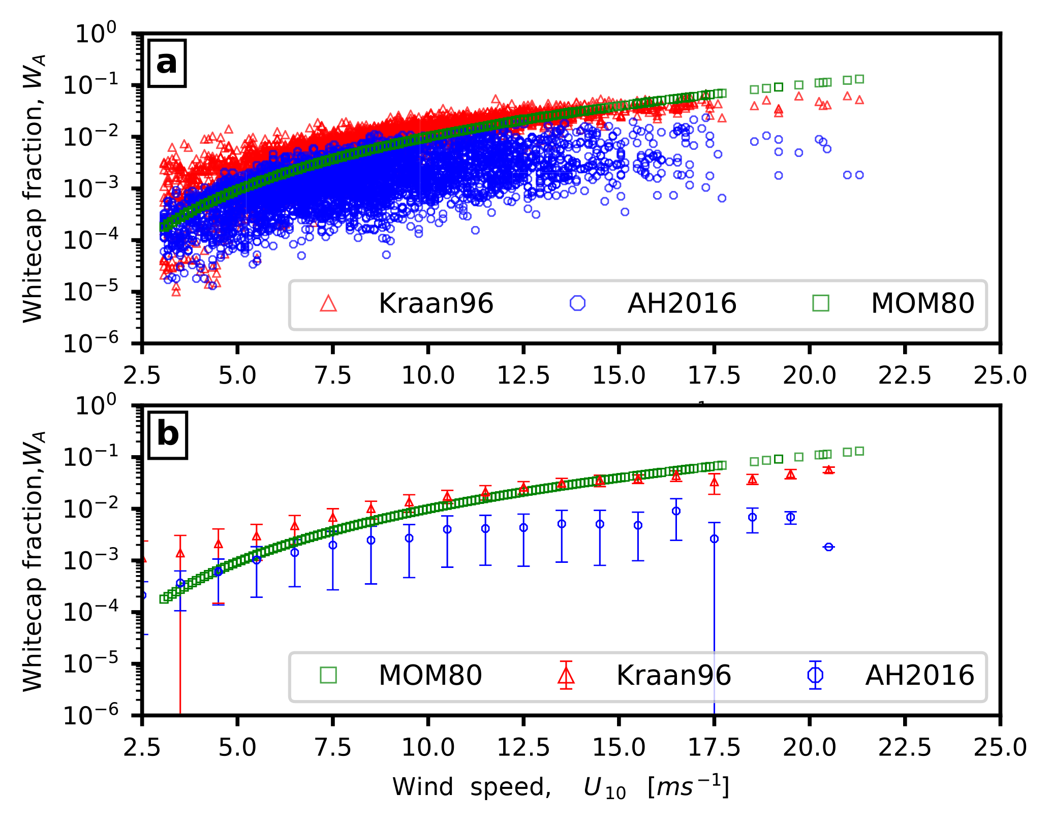
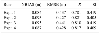
Figure 1 Wind speed dependence of the whitecap fraction (on log scale) obtained from (a) Kraan96 (Kraan et al., 1996), AH2016 (Anguelova and Hwang, 2016), and MOM80 (Monahan and Muircheartaigh, 1980). (b) As in (a), but data are binned in wind speed bins of 1 ms⁻¹ using data from buoy 46 001.

2.3 Spray flux parametrization

Following the arguments of our approach in Sect. 2.2, we model the sea spray fluxes using the wave energy dissipation. Here, we compare the whitecap fraction obtained from the wave energy spectrum with the model used in the present study to that of the model derived in the recent study of Anguelova and Hwang (2016). We also obtain the constant terms needed to obtain effective sea spray fluxes from the nominal spray fluxes calculated using the microphysical model described in the Sect. 2.2.

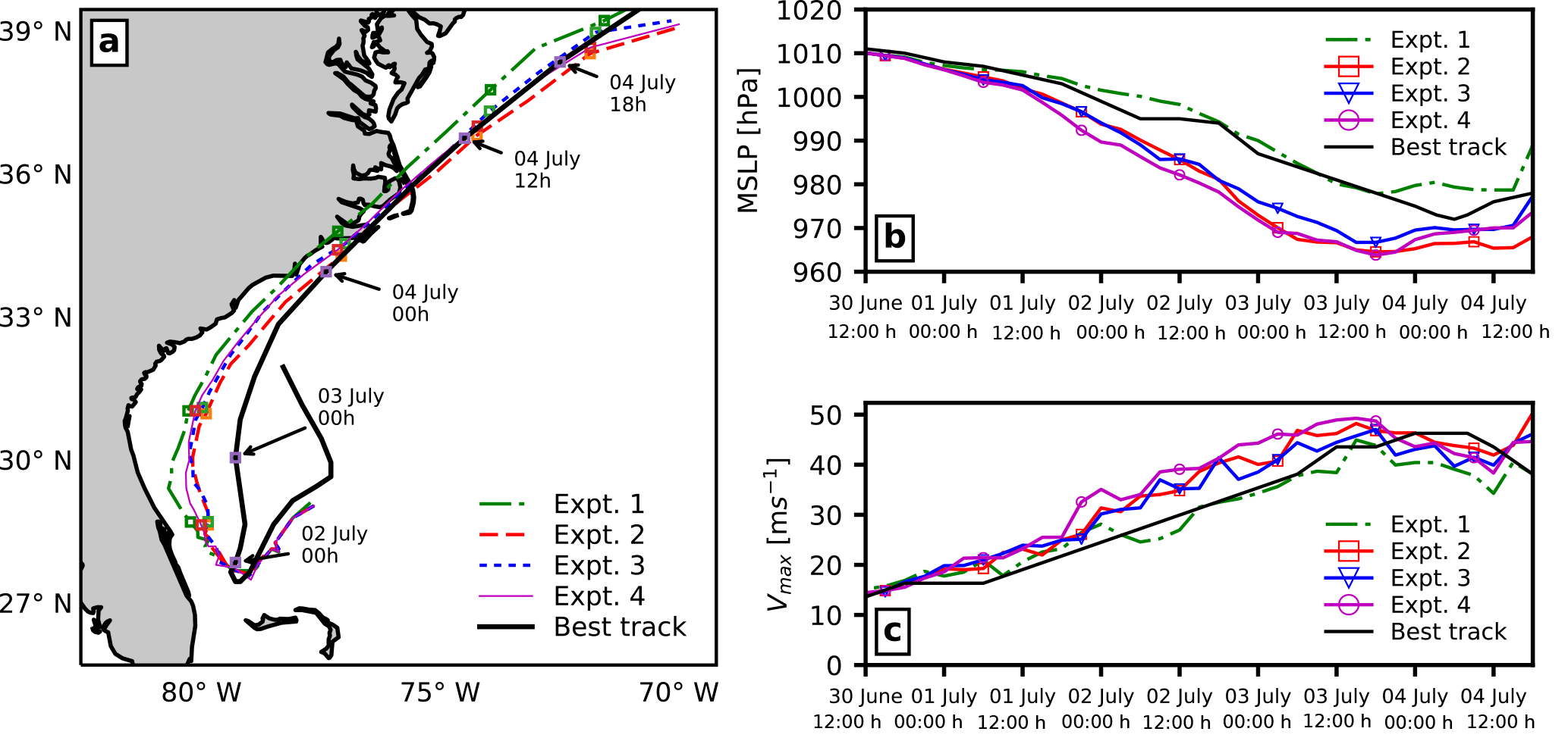
Figure 2 Comparison of (a) hurricane track, (b) time series of minimum sea level pressure (MSLP), and (c) time series of maximum wind speed (V_max) for the best track observed and four model experiments.

2.3.1 Whitecap fraction

As described earlier (Sect. 2.2.3), in the present study we estimate the SSGF using Eq. (15), whereby the whitecap fraction is obtained via Eq. (17). Anguelova and Hwang (2016) developed a parametric model for estimating the whitecap fraction; they applied their model to wave energy spectrum observations from National Data Buoy Center (NDBC) buoy 46 001 moored in the Gulf of Alaska at 56.3^∘ N, 147.9^∘ W. They also compared the results from their model to the photographic measurements of the whitecap fraction obtained in the Gulf of Alaska. It was shown that the whitecap fraction obtained from their model was comparable to the photographic observations. They also compared their results with the whitecap fraction model from Monahan and Muircheartaigh (1980), hereafter referred to as “MOM80”.

Figure 1 shows the comparison of the whitecap fraction obtained using Monahan and Muircheartaigh (1980), Anguelova and Hwang (2016), and Eq. (17); the results obtained from Eqs. (16) and (17) are comparable to those obtained by Anguelova and Hwang (2016). For details on the Anguelova and Hwang (2016) model, hereafter referred to as “AH2016”, the processing of the wave energy spectrum from buoy measurements, and their validation procedure, readers are referred to Anguelova and Hwang (2016). Figure 1b shows the same data (Fig. 1a) binned by wind speed. From Fig. 1, we can infer that the whitecap fractions obtained from Eqs. (16) and (17) are higher than that from the AH2016 model. We can also see that both methods show similar wind speed dependence, and at higher wind speeds, both give a lower whitecap fraction compared to the MOM80 model.

2.3.2 Estimation of sea spray fluxes

One implication of using the wave-state-dependent SSGF is the need to obtain the coefficients α,β, and γ as given in Eqs. (5) and (6). As described in Sect. 2.2.1, these coefficients are obtained from the statistical fit of total fluxes (spray-mediated and interfacial) to the fluxes from field observations. From Eqs. (7) and (8) we know that the sea spray fluxes depend on the volume flux of sea spray ejected in the DEL. For the purpose of this study, we followed the procedure described in Andreas and DeCosmo (1999) and utilized the HEXOS dataset (DeCosmo, 1991). Andreas et al. (2008) utilized the same HEXOS dataset together with the FASTEX dataset (Persson et al., 2005) to obtain the constant terms for the spray flux algorithm. Using a microphysical spray model with the COARE 2.6 bulk flux algorithm, we obtained α=7.7036, β=0.0, and γ=8.3202. We also calculated the correlation coefficients of modelled fluxes to the observed fluxes, where the correlation coefficient for sensible heat was 0.93 and for latent heat was 0.89. For the sake of brevity, we do not show the plots comparing the modelled fluxes to fluxes obtained from the observation dataset. Using Eqs. (5) and (6), the total enthalpy flux above the DEL can be written as

$$\begin{array}{}\text{(19)}& H_{\mathrm{S},\mathrm{T}}+H_{\mathrm{L},\mathrm{T}}=H_{\mathrm{L},\mathrm{I}}+H_{\mathrm{S},\mathrm{I}}+\mathit{\beta }\stackrel{\mathrm{‾}}{Q_{\mathrm{S}}}+\mathit{\gamma }\stackrel{\mathrm{‾}}{Q_{\mathrm{L}}}.\end{array}$$

When viewed in the context of the enthalpy flux, it can be said that only β and γ have an effect on the heat flux transfer from the ocean to the atmosphere. The values for the constants obtained in present study imply that only the spray-mediated latent flux has a role on the heat flux transfer. This is in contrast to the results obtained by Andreas et al. (2008) and Andreas and DeCosmo (1999), who found β to be a positive non-zero value. Also, it contradicts the conclusion that the spray sensible heat flux is the primary route by which spray affects the storm energy as stated in Andreas and Emanuel (2001). However, we want to stress that further investigation with more observation data is needed to support our earlier statement.

3 Methodology

The coupled modelling system used in this study consists of three components: a non-hydrostatic meteorological model (Weather Research and Forecasting, WRF), a third-generation wave model (DHI MIKE21 SW), and a model coupling interface. The model coupling interface is responsible for the re-gridding and exchange of data between the atmospheric and ocean wave model. These components and a brief overview of the coupling methodology are described below.

3.1 Atmospheric model

The atmospheric model within the coupled model is the Advanced Research (ARW) WRF version 3.4.1 (Skamarock et al., 2008). It is a non-hydrostatic atmospheric model which has been extensively used in operational forecasts, as well as for research purposes in both realistic and ideal configurations. The WRF model provides a suite of physics schemes and a variety of physical parametrizations for simulating a wide range of meteorological processes.

In the present study, the outer domain in the WRF model spans from 100 to 55^∘ W in a longitudinal direction and from 13 to 45^∘ N in a latitudinal direction. The outer domain has a horizontal resolution of 21.6 km and uses 41 vertical sigma levels. It covers the span shown in Fig. 3. There is also a stationary nest within the outer domain, which has a horizontal resolution of 7.2 km and uses 41 vertical levels. The initial and lateral boundary conditions for the atmosphere simulations were taken from the Modern-Era Retrospective analysis for Research and Applications, version 2 (MERRA-2) (Bosilovich et al., 2015) dataset, which has a resolution of $\mathrm{0.5}\times \mathrm{0.625}{}^{\circ }$ (50 km in a latitudinal direction). Due to the computational constraints, as well as the need to perform multiple simulations, we chose to apply only a one-way nesting approach, for which the feedback from the nested domain to the outer domain was turned off. The lateral boundary conditions from MERRA-2 to the outer domain were supplied at every 6 h interval and that from the outer domain to the nested domain at every 1 h interval. Also grid nudging was applied in the outer domain, so for the present study, we used the simplified Arakawa–Schubert scheme (Han and Pan, 2011) for convection, the Ferrier scheme (Rogers et al., 2001) for microphysics, the Rapid Radiative Transfer Model scheme (Mlawer et al., 1997) for long-wave radiation, the Dudhia scheme (Dudhia, 1989) for short-wave radiation, and the NOAH land surface model. The planetary boundary layer was modelled using the Yonsei University scheme (Hong et al., 2006), together with the Monin–Obukhov-theory-based surface layer scheme. We conducted a number of stand-alone simulations (not shown here) to choose the set of physics schemes which provide the best modelled track in comparison to the observed track.

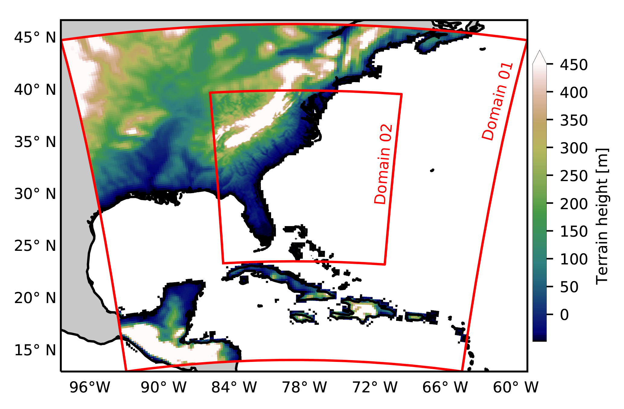
Figure 3 Horizontal extent and terrain elevation of atmosphere model domains in WRF, in which the horizontal resolution of the outer domain is 21.6 km while that of the inner domain is 7.2 km

3.2 Wave model

The ocean wave model used is the MIKE 21 SW (Sørensen et al., 2004; MIKEbyDHI, 2012). It is a third-generation spectral wind wave model based on an unstructured grid and solves the wave action density equation, in which it accounts for the wave growth, the wave energy dissipation due to whitecapping, the bottom friction, and the depth, as well as the non-linear wave–wave interaction. The spectral wave model can also account for wave–current interaction and ocean surface elevation; however these effects were not included in the present study.

The grid used in the ocean wave model comprises unstructured triangular meshes, in which the outer bounds of the wave domain are within the nested domain used in the atmospheric model grid. The model set-up uses 31 logarithmically spaced frequencies (0.04–0.7 Hz) and 24 equally spaced (15^∘) directions.

The bathymetry (see Fig. 4) used in the ocean wave model was constructed from the General Bathymetric Chart of the Oceans (GEBCO¹) 30 arcsec interval grid, for which the bathymetric data were interpolated on to the mesh nodes. Due to the low resolution of GEBCO data, in the coastal areas, data from the 3 arcsec U.S. Coastal Relief Model (CRM²) were also used. The lateral boundary conditions for the wave model were obtained from the well validated IOWAGA (Integrated Ocean Waves for Geophysical and Other Applications) (Stopa et al., 2016) global wave hindcast, conducted using the WAVEWATCH-III wave model (Tolman et al., 2002). The wave hindcast was constructed using the winds from the Climate Forecast System Reanalysis dataset (Saha et al., 2014).

3.3 Model coupling interface

The model coupling interface handles the interaction between the different model components. It is used for the remapping and interpolation of variables between different model components and contains the coupling physics module. The coupling physics includes the sea spray model and the wave boundary layer model. The schematic for different model components with respective variables used in the model coupling is provided in Fig. 5. In the present study, we only utilized the atmosphere–wave coupling aspect of the coupling interface, as the present study is intended to study the effects of the sea-state-dependent momentum and spray fluxes on a tropical cyclone (TC).

An unstructured grid allows a better representation of coastline features with minimal computational overhead compared to structured grids at comparable resolution; it creates disparity between the land/sea mask used by the atmosphere and the ocean/wave model if the model grids (i.e. atmosphere and ocean grid) use different kinds of meshes (e.g. unstructured and structured mesh). Also, the land/sea mask in the atmosphere model depends on both the model resolution as well as the land/sea mask used in the global model (from which the initial conditions have been obtained), while the land/sea mask in the ocean model is controlled by the quality of coastline. We primarily use a distance weighted remapping scheme (Jones, 1998) for the data exchange. However, as a consequence of the differences in the land/sea mask, at some grid locations, we also use nearest neighbour remapping (Watson, 1999) when exchanging data from the atmosphere to the ocean/wave model.

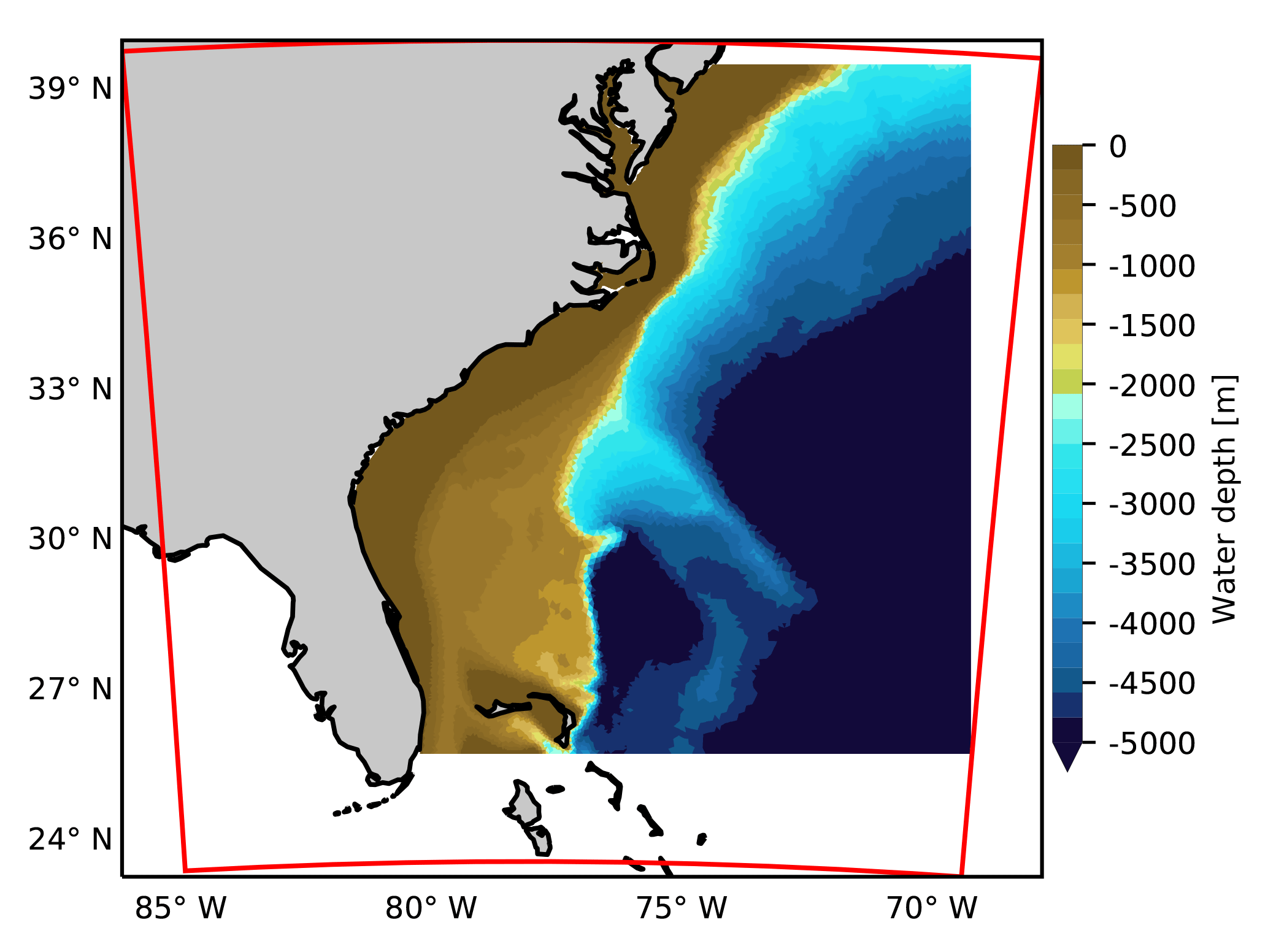
Figure 4 Horizontal extent and bathymetry of the wave model domain in MIKE 21 SW together with the extent of the inner domain used in the atmospheric model (red).

3.3.1 Atmosphere–wave coupling

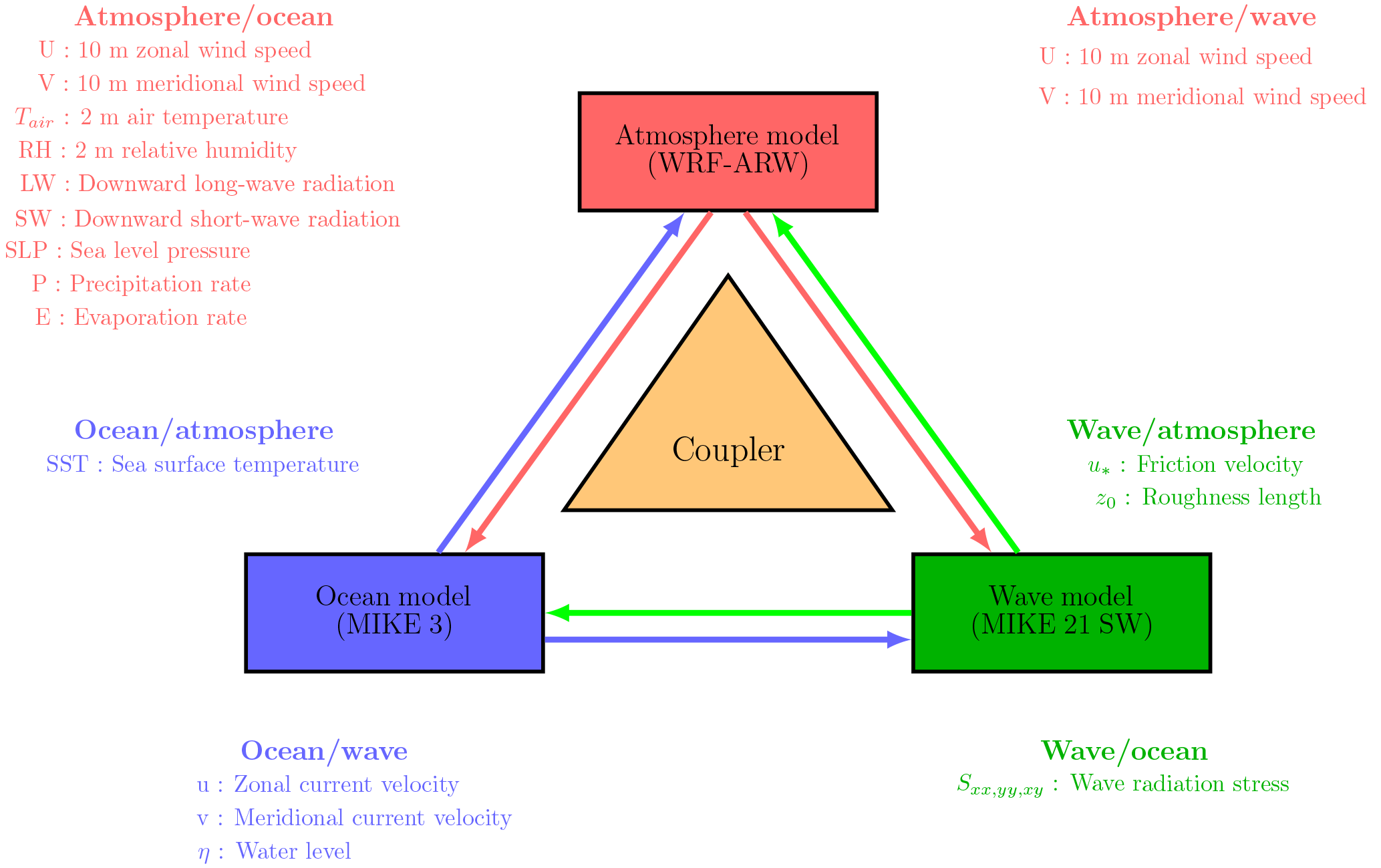
Figure 5 Schematics of coupled model components, where the atmosphere model (WRF), ocean model (MIKE 3) and wave model (MIKE 21 SW) interact through model coupling interface.

When waves are present, they affect the roughness length on the water surface, which affects the wind velocities and heat flux within the surface layer of the atmosphere. In this study, the atmosphere model provided the wind velocities at the height of 10 m to the wave model; the wave model in turn provides the surface roughness length to the atmosphere model. It is important to point out that the MIKE 21 SW model does not account for the stratification of the surface layer; i.e. it assumes that the surface layer is neutrally stratified. In order to realize the coupling between the atmosphere and the wave model, within the model coupling interface, we implemented the COARE 2.6 (Fairall et al., 1996) bulk flux algorithm, which adjusts the wind velocities obtained from the atmosphere model for neutral stratification.

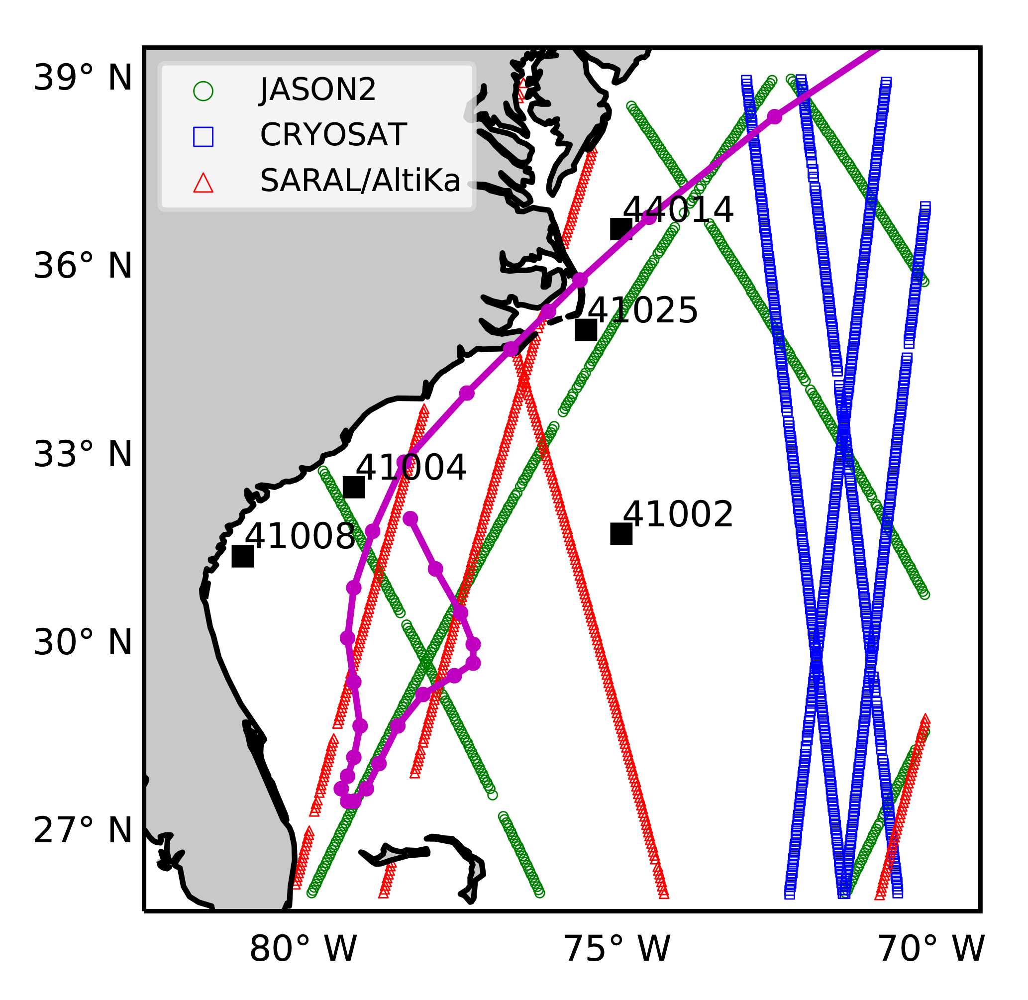
Figure 6 Altimeter tracks for JASON2 (green), CRYOSAT (blue), and SARAL/Altika (red) for the analysis period within the study region. The location of considered NDBC buoys are marked in black, and the observed track of Hurricane Arthur (2014) is overlaid in magenta.

3.4 Observation dataset sources

3.4.1 Wave buoys

In this study, surface measurements of wind and wave from two NDBC³ buoys from a number of wave buoys distributed along the United States east coast were used (see Fig. 6). The wave buoys provide measurements for wind speed, wind direction, air temperature, significant wave height (H_s), and wave period (T_p); the relative error in H_s is generally predicted to be (<5%) few percent.

3.4.2 Satellite data

Data for wind speed and H_s from the blended product of three different satellites, JASON-2, CRYOSAT, and SARAL (see Fig. 6), were obtained from the French Research Institute for Exploitation of the Sea (IFREMER). These satellites follow an orbit with a period of 10 days and provide along-track data with an approximate resolution of 6 km. The dataset from the satellite altimeter measurement has some limitations as given in Cavaleri and Sclavo (2006); the wind speed data are only reliable for 2 to 20 ms⁻¹, and additionally, the H_s measurements are not reliable beyond 20 m.

4 Model application

4.1 Synopsis of Hurricane Arthur (2014)

Hurricane Arthur was the first named storm of the 2014 hurricane season. It was first identified as a tropical depression at 00:00 UTC⁴ on 1 July 2014 by the National Hurricane Centre while it was located 70 nautical miles north of Freeport, Bahamas (Berg, 2015). It subsequently upgraded to a tropical storm at 12:00 UTC on 1 July 2014. By then the depression drifted westward to 60 nautical miles east of Ft. Pierce, Florida. Arthur, while located in a weak mid-level steering flow, meandered east of Florida till 2 July. On 2 July, a mid-level anticyclone developing over the western Atlantic caused Arthur to track northward, where it encountered low upper level winds and a warmer ocean temperature ($>{\mathrm{28}}^{\circ }$). Arthur strengthened while located east of Florida. It subsequently upgraded to a hurricane at 00:00 UTC on 3 July 2014, located 125 nautical miles east–southeast of Savannah, Georgia.

Later that day, Arthur turned north–northeastward, accelerating while moving between a ridge over the western Atlantic and a mid- to upper-level trough over the eastern United States. It continued to strengthen and reached its peak intensity of 85 knots at 00:00 UTC on 4 July 2014 just off the coast of North Carolina. At 03:15 UTC on 4 July 2014 it made landfall just west of Cape Lookout, North Carolina. After landfall, and crossing Outer Banks, Arthur accelerated northeastward over the western Atlantic on 4 and early 5 July. It subsequently transitioned to an extratropical cyclone at 12:00 UTC on 5 July just west of Nova Scotia.

4.2 Numerical experiments

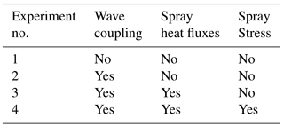
To evaluate the effects of ocean surface waves and ocean-wave-dependent sea spray on the tropical cyclone, four numerical experiments (Table 1) were conducted. In Expt. 1, we conducted an uncoupled atmosphere model run, which is also the control run for the present study. In the uncoupled run, the surface stress was estimated using Eq. (2). In Expt. 2, the effect of ocean surface waves was applied to the atmosphere model, in which the surface stress was obtained from the wave model. In Expt. 3 and 4, the sea spray fluxes were added to the coupled model runs; in Expt. 3 only the spray-mediated heat fluxes were applied, while in Expt. 4, both the spray-mediated heat and momentum fluxes were applied. All the numerical experiments were initialized at 00:00 UTC on 30 June 2014 and integrated for 120 h. This allows a 24 h spin-up period in the atmospheric model before Arthur strengthened to tropical depression at 00:00 UTC on 1 July 2014.

Table 1 Summary of numerical model experiments with different coupling configurations.

The model runs summarized in Table 1 do not include data assimilation, as the motivation was to investigate the response of the modelling system with the inclusion of different physical processes. To assess the validity of the model results, typical error metrics of normalized bias (NBIAS), root mean square error (RMSE), Pearson correlation coefficient (R), and scatter index (SI) were used, where the model estimates are expressed as y to the observed data x:

$$\begin{array}{}\text{(20)}& {\displaystyle }\begin{array}{rl}{\displaystyle }& {\displaystyle }\mathrm{NBIAS}={\displaystyle \frac{(\stackrel{\mathrm{‾}}{y}-\stackrel{\mathrm{‾}}{x})}{\sqrt{\frac{\mathrm{1}}{n}{\sum }_{i=\mathrm{1}}^n{x}_i^{\mathrm{2}}}}},\\ {\displaystyle }& {\displaystyle }\mathrm{RMSE}=\sqrt{{\displaystyle \frac{\mathrm{1}}{n}}{\sum }_{i=\mathrm{1}}^n(y_i-x_i{)}^{\mathrm{2}}},\\ {\displaystyle }& {\displaystyle }R={\displaystyle \frac{{\sum }_{i=\mathrm{1}}^n(y_i-\stackrel{\mathrm{‾}}{y})(x_i-\stackrel{\mathrm{‾}}{x})}{\left[\sqrt{\frac{\mathrm{1}}{n}{\sum }_{i=\mathrm{1}}^n(y_i-\stackrel{\mathrm{‾}}{y}{)}^{\mathrm{2}}}\sqrt{\frac{\mathrm{1}}{n}{\sum }_{i=\mathrm{1}}^n(x_i-\stackrel{\mathrm{‾}}{x}{)}^{\mathrm{2}}}\right]}},\\ {\displaystyle }& {\displaystyle }\mathrm{SI}={\displaystyle \frac{\mathrm{1}}{\stackrel{\mathrm{‾}}{x}}}\sqrt{{\displaystyle \frac{\mathrm{1}}{n}}{\sum }_{i=\mathrm{1}}^n{\left[(y_i-\stackrel{\mathrm{‾}}{y})-(x_i-\stackrel{\mathrm{‾}}{x})\right]}^{\mathrm{2}}}.\end{array}\end{array}$$

Here, the overbar denotes the mean, and n is the number of observations.

5 Results and discussion

5.1 Storm track and intensity

5.1.1 Storm track

A comparison of simulated hurricane tracks, obtained using the minimum sea level pressure, with the location of the storm centre from the best track and the model results is presented in Fig. 2a. The simulated storm tracks are generally consistent with the best track; the modelled storms first track southwestward and thereafter turn and move northward before making landfall. We notice that all the modelled storms are westward of the best track; however, when coupled with the wave model, the storm tracks improved. We can also see that the storm in the uncoupled model (Expt. 1) has a higher translation speed compared to the coupled atmosphere–wave model (Expt. 2–4) and best track data.

Although sea spray coupling (Expt. 3–4) does not have any appreciable effects on the model track, it does affect the translation speed of storm; in Expt. 3 (i.e. sea spray coupling with only heat fluxes) the storm moves faster compared to Expt. 4 (i.e. sea spray coupling with heat and momentum fluxes). Also, both the storms moved faster compared to Expt. 2.

5.1.2 Minimum sea level pressure (MSLP)

The time series of minimum sea level pressure (MSLP) are compared with the MSLP from best track data in Fig. 2b. Comparing the results of different numerical experiments (Expt. 1–4) indicates that the uncoupled model underestimates the storm intensity while the coupled model overestimates the storm intensity. The effect of both the sea spray heat and the momentum flux (Expt. 4) have little effect compared to the atmosphere–wave coupled model (Expt. 2). If only sea spray heat fluxes are considered (Expt. 3), the storm intensity is closer to the best track data. Including the wave and sea spray coupling (Expt. 2–4), the storm intensifies earlier compared to the uncoupled model (Expt. 1).

5.1.3 Maximum wind speed (V_max)

The temporal development of maximum wind speed at 10 m for the four experiments (Exit. 1–4) is shown in Fig. 2c. The effects of different model couplings on maximum velocity V_max are similar to that on the MSLP. We can see that the hurricane under-intensifies by up to $\approx \mathrm{10}{\mathrm{ms}}^{-\mathrm{1}}$ in the uncoupled (Expt. 1) model compared to best track data. Also, we note that the storm intensity improves when the atmosphere is coupled with waves (Expt. 2–4). However, in contrast to Sect. 5.1.2, from Fig. 2 it is evident that the V_max values are better modelled in Expt. 2 and Expt. 4.

5.2 Model validation

5.2.1 Wind observations

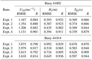
To further investigate the effects of ocean waves and sea spray, we compare the computed wind speeds with the winds measured at NDBC buoys. Figure 6 shows the location of the buoys considered in reference to the track of Arthur. We can see that buoy 41 002 is located offshore, while buoy 44 014 is located along the track of Arthur. Both coupled and uncoupled models in the present study overpredict the intensity of the storm at 44 014, while they perform well at buoy 41 002 (Fig. 7a); however, we do note that the wave coupling in the atmosphere results in improved timing of the storm at buoy 44 014 (Fig. 7b). We also see that coupling the sea spray (Expt. 3–4) results in lower V_max at the buoy location, though when the spray-mediated momentum flux is applied together with spray-mediated heat fluxes (Expt. 4), both the timing as well as the buoy location are improved. Additionally, Fig. 8 compares the wind direction at buoy 41 002 and 44 014 obtained from the four numerical experiments. Furthermore, the computed statistics for both wind speed and wave parameters (i.e. wave height H_s and wave period T₀₂) are given in Table 2. The coupling of ocean surface wave reduces (increase) the error in wind speed at buoy 44 014 (41 002); however, when sea spray fluxes are applied, this reduction in error diminishes. Moreover, when comparing both the RMSE and correlation between wave measurements and data obtained from various numerical experiments, it can be said that the coupling of the wave model improves the model results. It can also be construed from Table 2 that it is necessary to account for both the spray-mediated heat and the momentum flux, as when only spray-mediated heat fluxes are accounted for, there is a noticeable reduction in the correlation coefficient with an increase in RMSE.

Table 2 Root mean square error (RMSE) and correlation coefficient (R) for mean wind speed U₁₀ at 10 m elevation, significant wave height H_s, and wave period T₀₂ between model experiments and buoys 41 002 and 44 014.

5.2.2 Wave observations

During a hurricane, the waves are not only affected by the winds but also by the hurricane intensity and translation speed among other factors. Figures 9 and 10 show the comparison of significant wave height H_s and mean wave period T₀₂ for the four different model experiments with the buoy measurements.

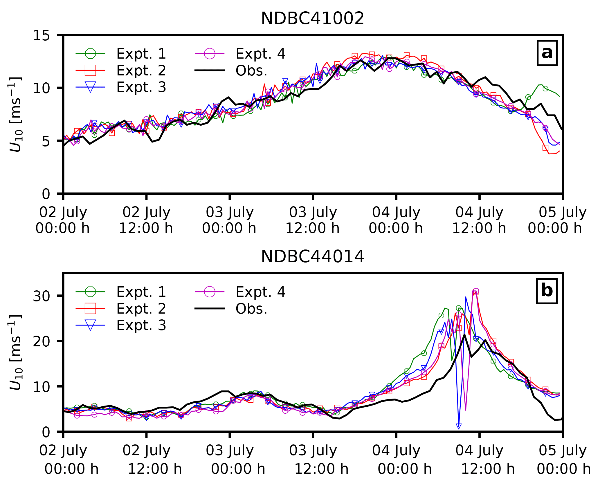
Figure 7 Comparison of coupled model results with NDBC buoys (a) 41 002 and (b) 44 014 for mean wind speed U₁₀ (ms⁻¹) at 10 m elevation.

Figure 8 As in Fig. 7, but for wind direction.

Figure 9 As in Fig. 7, but for significant wave height H_s (m).

Figure 10 As in Fig. 7, but for wave period T₀₂ (s).

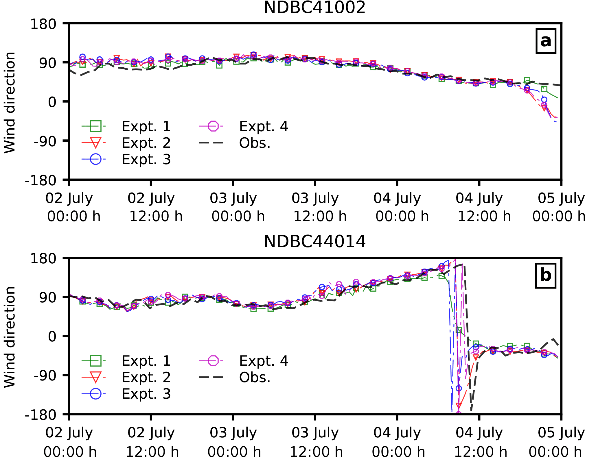
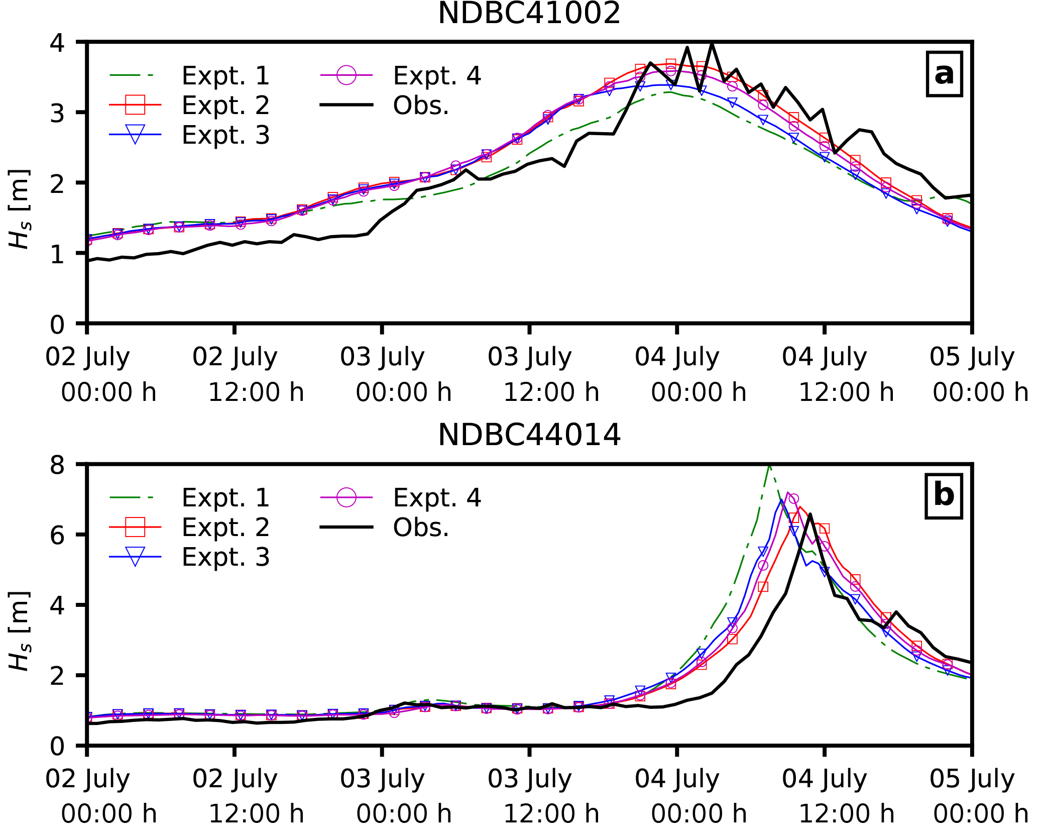
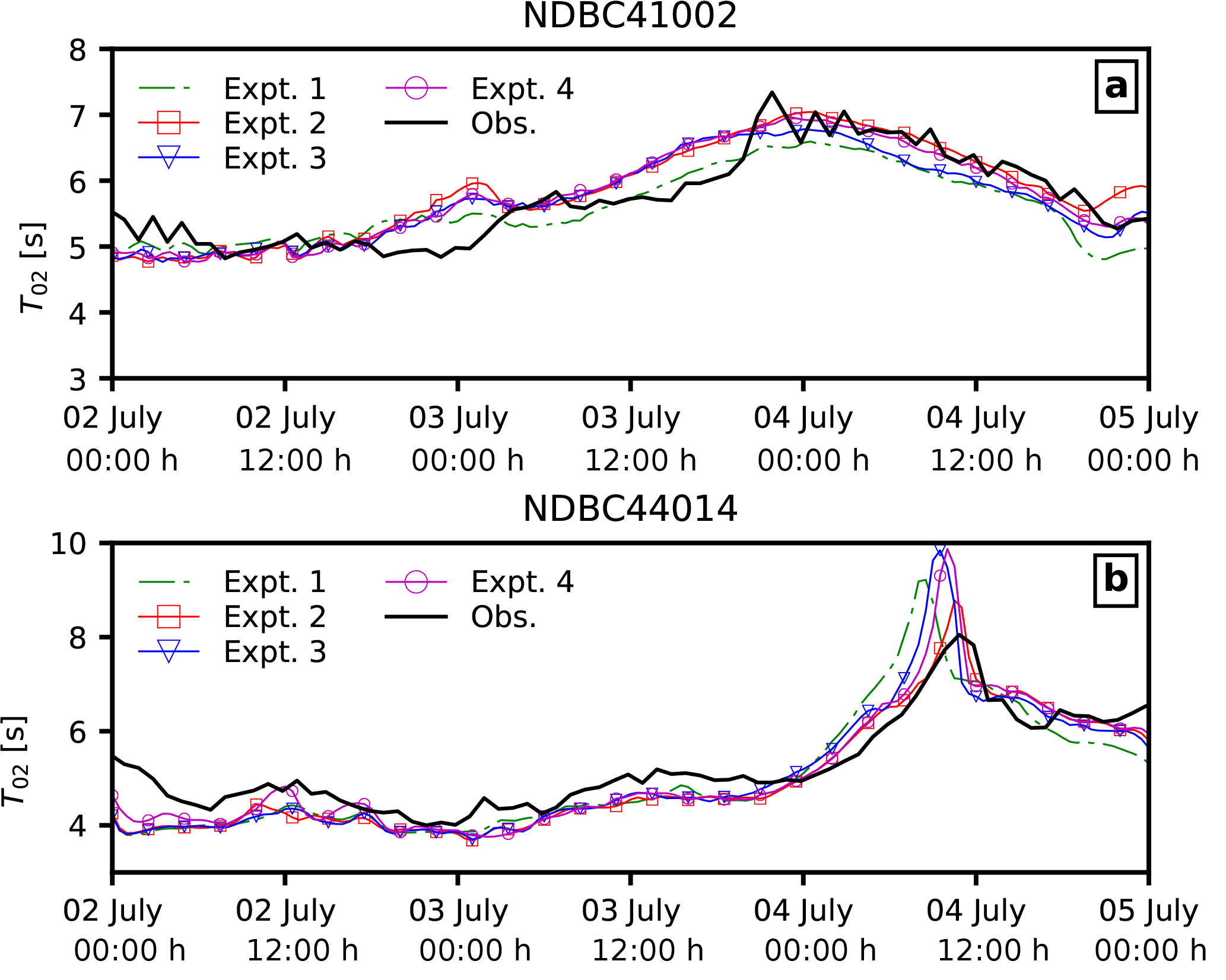
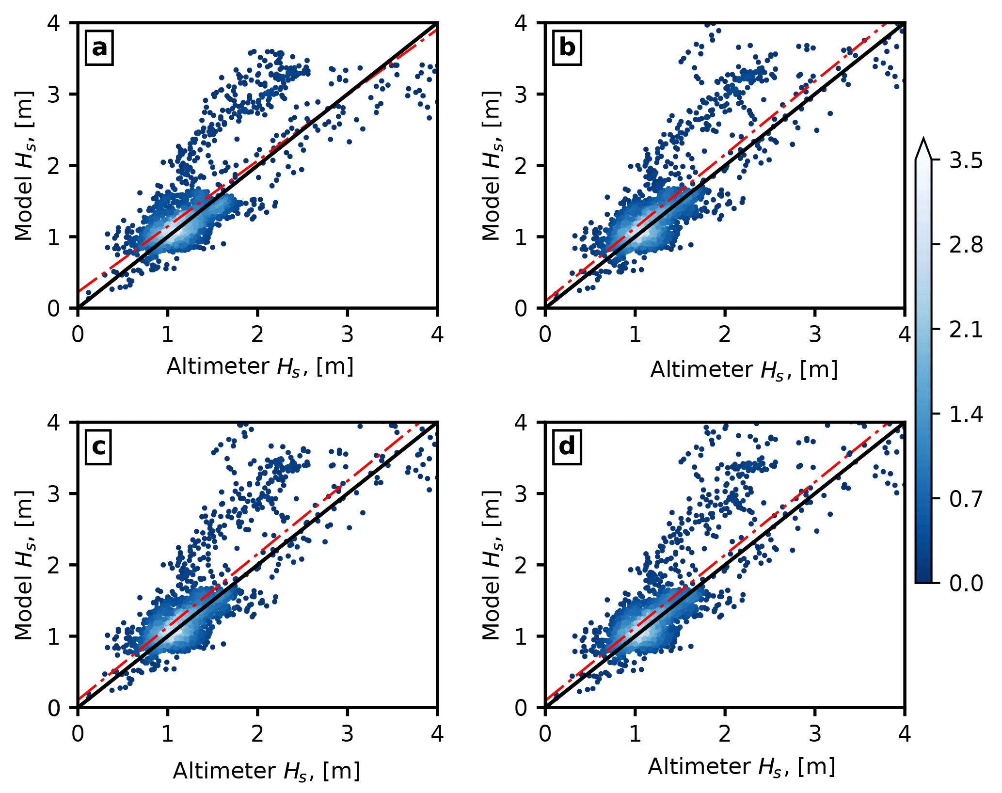
Figure 11 Scatter plot of modelled versus observed H_s for (a) Expt. 1, (b) Expt. 2, (c) Expt. 3, and (d) Expt. 4 during 30 June to 5 July within the coupled model domain. The colour bar indicates the number of occurrence in each 0.1 m bin on a logarithmic scale. The solid black line represents the ideal fit of model and measurements, while the dashed red line represents the linear fit of the data.

The significant wave height H_s and wave period T₀₂ were rather well estimated when the atmosphere model was coupled with waves (Expt. 2–4) compared to the uncoupled model (Expt. 1). However, the size of storm-induced wave fields in the coupled model (Expt. 2) indicates that the storm size is bigger compared to the uncoupled model and buoy measurements.

Also, when sea spray effects are included in the coupled model, the modelled peak H_s values are similar to that of measurements; the hurricane passes the buoy locations earlier than observed. We attribute the bias in timing of the storm passage to the translation speed of the storm, whereby a higher translation speed can result in an increased effective fetch, thereby giving higher wave heights.

We also compared the collocated significant wave heights from model experiments to the satellite-altimeter-derived wave heights (Fig. 11). This was done by computing the closest model data point (both in space and time) to each satellite observation point. This allows us to evaluate the spatial and temporal variation of the wave field due to different processes investigated here. The computed statistics of the modelled wave heights compared to the altimeter data are given in Table 3. When the wave effects were included in the wave model, a higher correlation and lower scatter compared to altimeter data was observed. When sea spray was included in the coupled atmosphere–wave model runs, we can see that including the spray-mediated momentum flux improves the model results.

Table 3 Statistical comparison of altimeter-derived and wave-model-derived significant wave height H_s; normalized bias (NBIAS), root mean square error (RMSE), Pearson correlation coefficient (R) and scatter index (SI).

It is noteworthy that there are only minor differences between the output of uncoupled and coupled model experiments at lower wave heights; however, only coupled models were able to capture the higher wave heights. It is also worth mentioning that apart from modelling uncertainties, the bias in model results can arise from the differences in temporal and spatial resolution of the wave model and the satellite altimeter. Furthermore, for the comparison presented in Fig. 11, no spatial (or temporal) smoothing of altimeter data was carried out. This is due to the use of an unstructured grid in the present study for the wave model set-up.

5.3 Surface fluxes

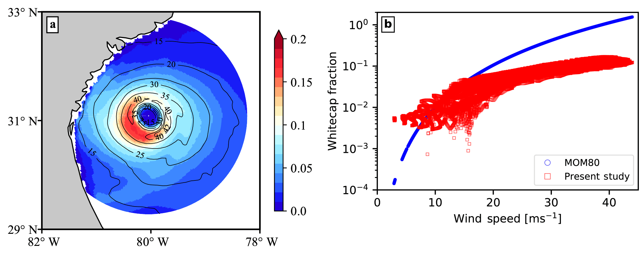
Figure 12 Computed whitecap fraction from Expt. 4 at 00:00 UTC on 3 July 2014. (a) Distribution of the whitecap fraction with contours of mean wind speed U₁₀. (b) Comparison of the whitecap fraction (on log scale) with mean wind speed U₁₀.

Figure 13 Plan views of surface sensible heat flux for (a) Expt. 1, (b) Expt. 2, (c) Expt. 3, and (d) Expt. 4 at 00:00 UTC on 3 July 2014. The black arrow indicates the hurricane translation direction over a 3 h interval.

Figure 14 As in Fig. 13, but for the surface latent heat flux.

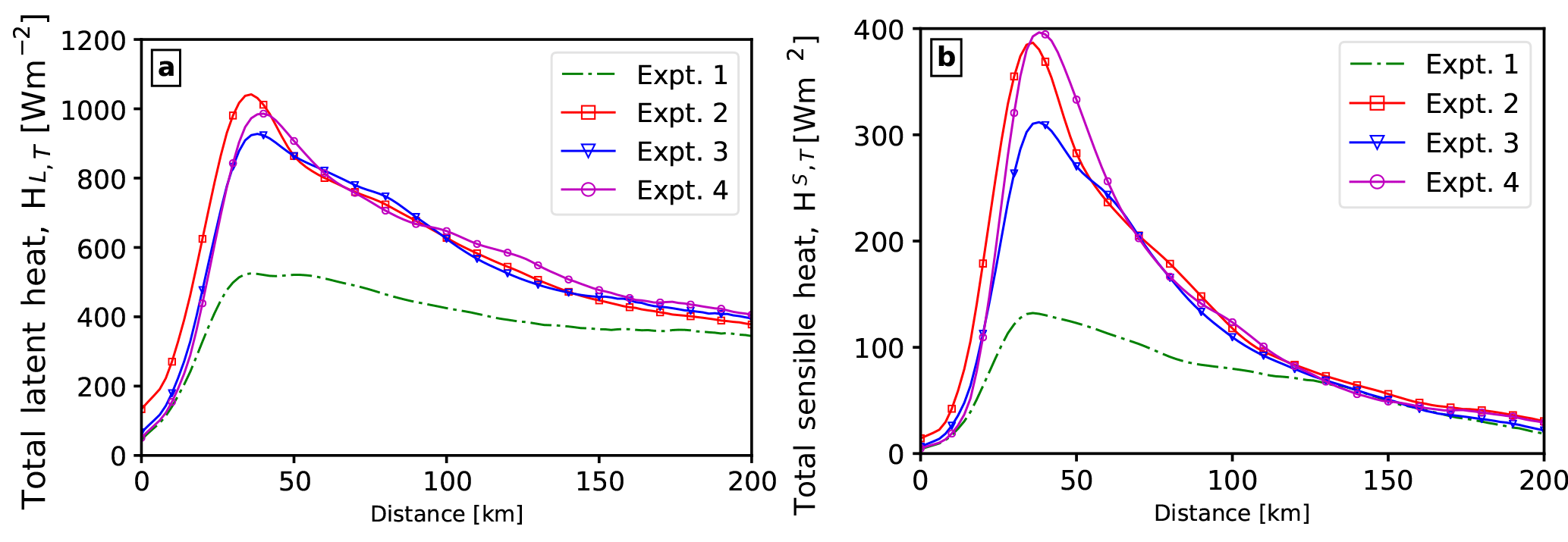
Figure 15 Radial distribution of the azimuthal averaged total (a) latent heat flux and (b) the sensible heat flux at 00:00 UTC on 3 July 2014.

Figure 12 shows the distribution of the wave-model-dependent whitecap fraction computed from Expt. 4 at 00:00 UTC on 3 July 2014. Figure 12a presents the spatial distribution of the whitecap fraction with wind speed contours, while Fig. 12b shows a comparison of the whitecap fraction obtained from the wave energy spectrum with the widely used MOM80 formula. It should be noted that the results given in Figs. 12–15 are presented on a storm relative grid with 2 km spacing in the radial direction and a 1^∘ spacing in the azimuthal direction. Here, the storm relative grid was created using storm centres which correspond to the location of the minimum sea level pressure. The whitecap fraction (Fig. 12) and surface heat fluxes (Figs. 13–15) obtained from the wave and atmosphere models were interpolated onto the aforementioned storm relative grid. Furthermore, only data points that are within 200 km of the storm centre and over the ocean are presented. From Figs. 1 and 12b, for wind speeds between 10 and 20 ms⁻¹, whitecap fractions obtained from MOM80 and Eqs. (16)–(18) show similar wind speed dependence; however, when extended to wind speeds present during hurricanes, whitecap fractions obtained from MOM80 are substantially higher, with a whitecap fraction of 1.0 at 40 ms⁻¹. This seems to show that at wind speeds greater than 40 ms⁻¹, the whole sea surface will be covered in whitecaps, whereas only 20 % of the sea surface is covered when the whitecap fractions are computed from wave energy dissipation.

Until now, we have only discussed the wind speed dependence of the whitecap fraction. When looking at the spatial distribution of the whitecap fraction in relation to the wind speed (see Fig. 12), it can be noted that the peak of the whitecap fraction is in the rear left quadrant of the hurricane translation direction (see black arrow in Fig. 13d), whereas the peak of the wind intensity is in the front right quadrant of the hurricane. This shows that within the coupled model used in the present study, not only was the volume of sea spray droplets generated altered, but also the spatial spread of the sea spray volume flux was modified. This is noteworthy, as when sea spray production is parametrized using MOM80 (where the whitecap fraction $W_{\mathrm{f}}=\mathrm{3.8}\times {\mathrm{10}}^{-\mathrm{6}}{U}_{\mathrm{10}}^{\mathrm{3.41}}$), the peak of the whitecap fraction will be collocated with the peak of wind speed. It is important to keep in mind that the results presented in Fig. 12b merely highlight the fact that in most studies the MOM80 model is applied beyond the range of its validity, as is the case in Fig. 12b.

The effects of including spray-mediated heat fluxes as well as ocean surface waves on the enthalpy fluxes (i.e. sensible and latent heat flux) are shown in Figs. 13–15. Here, we first compare the total sensible heat flux (Fig. 13), then the total latent heat flux (Fig. 14), and eventually their azimuthal averaged radial variation in Fig. 15. The heat fluxes are presented for 00:00 UTC on 3 July 2014 because the storm centres were collocated (see Fig. 2a).

It is evident from the comparison of sensible and latent heat flux obtained from the uncoupled atmosphere model (Expt. 1) and the ocean wave coupled atmosphere model (Expt. 2) that coupling ocean waves with the atmosphere results in a substantial increase in sensible and latent heat fluxes. Using Fig. 13 and 14, it can be argued that the increase in heat fluxes is largely due to wave-induced surface roughness, rather than any air–sea temperature difference that might arise due to the usage of the fixed sea surface temperature field. These results are inline with the arguments given in Janssen et al. (2001), in which it was suggested that the increased surface roughness will enhance the surface heat fluxes, causing vortex stretching and thus intensifying the storm. Recent studies by Montgomery et al. (2010) and Kilroy et al. (2017) investigated the effects of surface friction on the genesis and intensification of idealized tropical cyclone. Both of the studies concluded that increasing the coefficient of drag C_d up to a certain value ($\mathrm{2}\times {\mathrm{10}}^{-\mathrm{3}}$ in former study) aids in the intensification of the tropical cyclone. These results are noteworthy, as they refute the “conventional wisdom” that increasing C_d should weaken the tropical cyclone. However, it should also be kept in mind that in the studies by Montgomery et al. (2010) and Kilroy et al. (2017), the C_d values are kept constant over the whole model domain, which is both unphysical and in contrast with our study, in which the C_d depends on the wave state.

By comparing Fig. 13b and c, it can be noticed that when only spray-mediated heat fluxes (Expt. 3) are added, there is a reduction in the sensible heat flux as well as a broadening of the storm core compared to Expt. 2. Furthermore, adding both spray-mediated heat and momentum fluxes (Expt. 4) results in a higher sensible heat flux (see Fig. 13d) compared to Expt. 3. Besides the differences in the sensible heat flux, there are also differences in the location of the maximum sensible heat flux with respect to the storm centre.

Contrary to the assumption that applying the spray-mediated heat flux will intensify the hurricane, these results show that the interaction between the sea spray and the hurricane is rather more intricate, whereby both the thermodynamic and dynamic processes play different roles. For instance, coupling waves with the atmosphere model increases the surface roughness, which results in the intensification of the hurricane. Increased surface roughness may however also decelerate the hurricane, as seen in Fig. 2, causing it to stay on the warmer ocean for a longer duration.

The radial distributions of azimuthally averaged total latent and sensible heat fluxes for the four model experiments are presented in Fig. 15. It is clearly noticeable that in all the experiments, the maximum values of heat fluxes (i.e. sensible and latent heat flux) are in the high wind region (i.e. radius of 20 to 75 km). Also, the maximum value of the latent heat flux in Expt. 2–4 is twice that of Expt. 1, whereas the maximum value of the sensible heat flux in Expt. 2 and 4 is thrice that of Expt. 1. In Expt. 3 it is 2.5 times that of Expt. 1. Besides the effects of coupling the wave model with the atmosphere model (Expt. 2), the effects of sea spray on the sensible and latent heat fluxes can also be noticed. In the case of sea spray heat fluxes (Expt. 3), there is a noticeable reduction in the maximum value of sensible and latent heat fluxes compared to Expt. 2. However when both spray-mediated momentum and heat fluxes are considered (Expt. 4), there is a reduction in the maximum latent heat flux, while there is an increase in the maximum sensible heat flux compared to Expt. 2. It should also be pointed out that these difference in heat fluxes (between Expt. 2 and 4) are only in the high wind region, with negligible effects at higher radii. In addition to affecting the value of heat fluxes, sea spray (Expt. 3–4) also causes a slight broadening of the core size compared to Expt. 2.

To examine the effects of coupling the wave model and sea spray on the vertical structure of the hurricane, Fig. 16 shows the azimuthally averaged radius–height cross-section of temperature (Fig. 16b, d, f) and mixing ratio q (Fig. 16a, c, e) anomaly. The radius–height cross section utilizes the storm centre located at the surface for all the vertical levels so as to construct a storm relative grid. The anomaly fields were calculated by subtracting azimuthally averaged fields for Expt. 1 from those for Expt. 2–4. For Expt. 2 (Fig. 16b) a strong positive anomaly extends from z=4 to 16 km and from r= 0 to 140 km, whereas there is a weak negative anomaly in the near-surface region at radii greater than 40 km. The warming in the upper air region within the hurricane core (i.e. near the eye wall) in Expt. 2 can be attributed to the increase in surface heat fluxes. Comparing Fig. 16b and d, we can see that, when sea-spray-mediated heat fluxes are added, there is a reduction in upper level warming in the core region, whereas there is enhanced cooling in near-surface layers at radii greater than 4 km. Also, broadening of the warm anomaly in the core can be noted; the edge of the warm anomaly in Fig. 16b has shifted rightwards compared to Fig. 16a. This broadening of the warm anomaly and the increased cooling in near-surface layers can be associated with the decreased storm intensity. Figure 16d shows the temperature anomaly when the spray-mediated momentum flux is added together with the spray heat fluxes. The first key effect is the enhancement of the warm anomaly in the upper levels compared to Expt. 3. Although the broadening of the core is still present, there has been a slight reduction in the cooler region compared to Expt. 3.

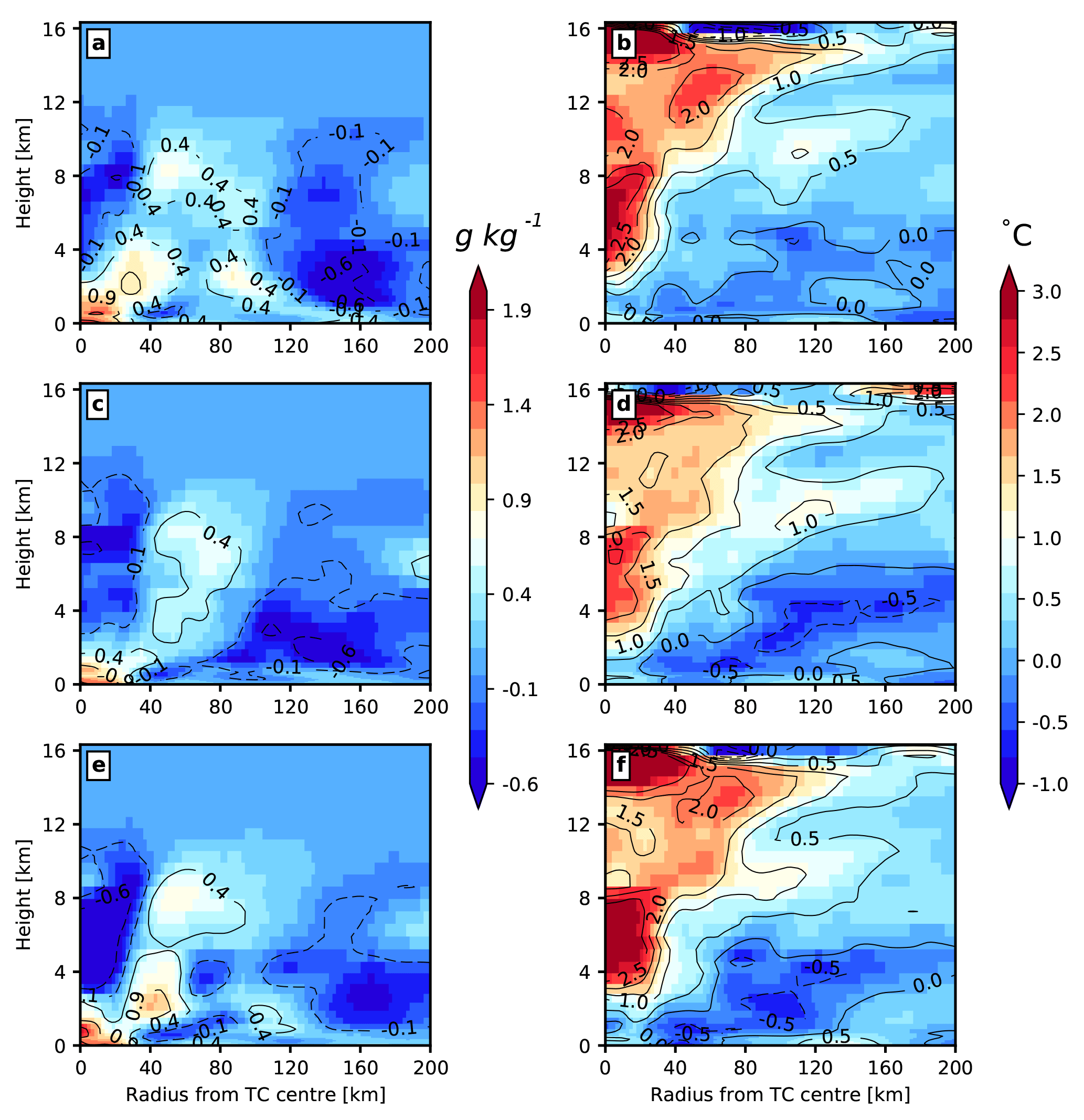
Figure 16 Height–radius cross sections of the difference of the azimuthally averaged mixing ratio (left) and temperature (right), for (a, b) Expt. 2, (c, d) Expt. 3, and (e, f) Expt. 4. The difference was calculated by subtracting the azimuthal averaged quantity for Expt. 1 from the respective coupled model results at 00:00 UTC on 3 July 2014.

Figure 16a shows the mixing ratio anomaly for Expt. 2 relative to Expt. 1 (i.e. uncoupled atmosphere model run). A broad region of positive anomaly can be noted, extending from radii of 60 to 160 km. Also, just above this region at radii greater than 120 km, a large region of a negative anomaly can be noticed. The largest positive anomalies are in the near-surface region in all the experiments, with the maximum occurring in the core region. When the spray heat fluxes are added (Fig. 16b), the negative q anomaly has shifted from radii of 120 to 80 km, though with a considerable downward shift of the vertical extent from 12 to 6 km. However, when both the spray heat and momentum fluxes are utilized (Fig. 16c), the extent of the negative anomaly has shifted back to a 120 km radial location from 80 km. Also, worth noting is the increase in the negative q anomaly within the eye wall region, where the q values have decreased by −0.6 compared to −0.1g kg⁻¹ seen in Fig. 16a and b.

6 Summary

This study investigated the effects of air–sea interaction on the life cycle of Hurricane Arthur (2014) that traversed through the North Atlantic Ocean, made landfall in north Carolina, then re-emerged over the western Atlantic. and eventually underwent transition to an extratropical storm. More specifically, this study explored the role of ocean surface waves and sea-spray-mediated heat and momentum fluxes on the structure and intensity of the aforementioned tropical cyclone.

There has been limited work in assessing the effects of sea-spray-mediated fluxes using a coupled atmosphere–wave model in which the sea spray generation was modelled using wave energy dissipation. Furthermore, most of the previous studies used bulk approximations of sea spray fluxes when used in conjunction with the atmosphere or a coupled atmosphere–wave model. The aforesaid bulk approximations were formulated as a function of surface wind speed or friction velocity. In the present study, a consistent approach for incorporating sea spray fluxes without relying on bulk approximations was presented. Moreover, a comparison of the whitecap fraction obtained from wave energy dissipation with the widely used MOM80 model (Monahan and Muircheartaigh, 1980) and recently formulated AH2016 model (Anguelova and Hwang, 2016) was presented. It was shown that the method adopted in the present study results in a whitecap fraction comparable to the results reported by Anguelova and Hwang (2016), while a substantially lower whitecap fraction was found at higher wind speeds compared to MOM80. Due to the limitations in the sea spray microphysical model, a new set of coefficients for incorporating nominal spray fluxes using the HEXOS dataset was obtained.

To investigate the role of surface waves and sea spray fluxes, a two-way coupled atmosphere–wave model was utilized. The coupled model was developed using a flexible coupler, in which different processes (such as sea spray physics) were integrated at the coupler level. Within the coupled model, sea spray fluxes were incorporated as the discrete contribution of a spectrum of spray droplets. The spray droplet generation was modelled using the ocean wave energy dissipation due to whitecapping. The results from four different model simulations were analysed to elucidate the effects of wave-induced surface roughness and spray-mediated heat and momentum fluxes on the distribution of sensible and latent heat as well as the temperature and mixing ratio among different model coupling scenarios. Furthermore, the wave model results from different numerical experiments were compared with the measurements obtained from floating offshore buoys and a satellite altimeter.

As illustrated in Fig. 2, the model employed in the present study captures the life cycle of the simulated TC relatively well. The uncoupled atmosphere model results in a somewhat weaker TC, while the coupled model results in a somewhat stronger TC compared to the best track data. Furthermore, all the simulated TCs traverse westward of the best track data; however, when the atmosphere model is coupled with a surface wave model, the TC track shifts east of the uncoupled model track. Also, compared to the uncoupled atmosphere model, the coupled model-simulated storms are able to attain a maximum velocity similar to that of best track data, but all the simulated storms attain maximum intensity almost 12 h before that observed in best track data. Despite all the foregoing differences, it behoves us to argue that the numerical experiments performed in the present study are adequate for conducting a preliminary investigation of the role of ocean waves and sea spray fluxes.

Moreover, in the recent literature, a number of explanations have been associated with the bias in the simulated TC tracks. These include the effects of the dataset used for the model initialization, the initialization time of the model run, the atmosphere model resolution, and the physics scheme used for cumulus parametrization. All of these are topics of active research; a number of advanced techniques such as the ensemble Kalman filter and advanced data assimilation have been developed to alleviate the effects of the initial condition error, and TC bogussing has been applied to reduce the bias due to the initialization time. Large eddy simulation and super-parametrization methods are being used to improve the cumulus parametrization in numerical models. It is arguable that running the same numerical experiments with different initial conditions (e.g. ERA-Interim or GFS Final analyses) would be useful to assess the validity of the results presented here; however, though such tests are beyond the scope of present study, they are recommended for future work.

Including the sea-state-dependent surface roughness increases the sensible and latent heat flux exchange within the surface layer. As the present study does not couple an ocean model, this increase in surface heat fluxes is therefore presumably from the increased surface friction velocity. Moreover, in the present study, the sea spray fluxes (or the SSGF) depend on the wave energy dissipation due to whitecapping; therefore it is not possible to distinguish between the effects of coupling sea spray fluxes and ocean surface waves. However, the results presented here do underscore the significance of the friction velocity in modulating the storm intensity. Furthermore, the results presented here also allude to the uncertainty associated with the inclusion of sea spray fluxes; the limitations are due to the lack of observation data at higher wind speeds and the limited understanding of the underlying physical processes necessary for modelling sea spray fluxes.