Volcanic ash modeling with the NMMB-MONARCH-ASH model: quantification of offline modeling errors

Volcanic ash modeling systems are used to simulate the atmospheric dispersion of volcanic ash and to generate forecasts that quantify the impacts from volcanic eruptions on infrastructures, air quality, aviation, and climate. The efficiency of response and mitigation actions is directly associated with the accuracy of the volcanic ash cloud detection and modeling systems. Operational forecasts build on offline coupled modeling systems in which meteorological variables are updated at the specified coupling intervals. Despite the concerns from other communities regarding the accuracy of this strategy, the quantification of the systematic errors and shortcomings associated with the offline modeling systems has received no attention. This paper employs the NMMB-MONARCH-ASH model to quantify these errors by employing different quantitative and categorical evaluation scores. The skills of the offline coupling strategy are compared against those from an online forecast considered to be the best estimate of the true outcome. Case studies are considered for a synthetic eruption with constant eruption source parameters and for two historical events, which suitably illustrate the severe aviation disruptive effects of European (2010 Eyjafjallajökull) and South American (2011 Cordón Caulle) volcanic eruptions. Evaluation scores indicate that systematic errors due to the offline modeling are of the same order of magnitude as those associated with the source term uncertainties. In particular, traditional offline forecasts employed in operational model setups can result in significant uncertainties, failing to reproduce, in the worst cases, up to 45–70 % of the ash cloud of an online forecast. These inconsistencies are anticipated to be even more relevant in scenarios in which the meteorological conditions change rapidly in time. The outcome of this paper encourages operational groups responsible for real-time advisories for aviation to consider employing computationally efficient online dispersal models.

1 Introduction

Volcanic ash modeling systems are used to simulate the atmospheric dispersion of volcanic ash and to generate operational short-term forecasts to support civil aviation and emergency management. These systems are vital in efforts to prevent aircraft flying into ash clouds, which could result in catastrophic impacts (e.g., Miller and Casadevall, 2000; Prata and Tupper, 2009). The aviation community is concerned about the detection and tracking of volcanic ash clouds to provide timely warnings to aircrafts and airports. In the event of an eruption, the individual Volcanic Ash Advisory Center (VAAC) responsible for the affected region combines ash cloud satellite observations and dispersal simulations to issue periodic volcanic ash advisories (VAAs). These are text and graphical products informing on the extent of the ash clouds at relevant flight levels and their forecasted trajectories at 6, 12, and 18 h ahead that are updated periodically or whenever significant changes occur in the eruption source term. All this information is used to ensure flight safety by supporting critical decisions such as closure of ash-contaminated air space and airports or diversion of aircraft flight paths to prevent encounters. The noteworthy economic impact and social disruption of these air traffic restrictions are, therefore, directly associated with the accuracy of the volcanic ash cloud detection and modeling systems.

Volcanic ash modeling systems require (i) a source term to characterize the emission of ash, (ii) a meteorological model (MetM) for the description of the atmospheric conditions, and (iii) a volcanic ash transport and dispersal model (VATDM; e.g., Folch, 2012) to forecast the particle transport and deposition mechanisms. The MetM and the VATDM can be coupled either online or offline. In an offline modeling system, the MetM runs a priori and independently from the VATDM to produce the required meteorological fields at regular time intervals, e.g., every 1 to 6 h for typical mesoscale and global operational MetM outputs, respectively. Meteorological fields are then furnished to the VATDM, which commonly assumes constant values for these fields during each time coupling interval or, at most, performs a linear interpolation in time. This approach is convenient in terms of computing time because different VATDM model executions are possible without rerunning the meteorological component, e.g., to update the source term whenever the eruption conditions vary, for inverse modeling of ash emissions (e.g., Marti et al., 2016; Webster et al., 2012), or to perform an ensemble forecast (e.g., Galmarini et al., 2010) in which all the ensemble members share the same meteorological conditions. However, offline MetM and VATDM coupling introduces model and numerical errors due to non-synchronized time stepping, use of unaligned grids and projections, and/or inconsistencies in the numerical schemes. In contrast, in an online modeling system, the MetM and the VATDM run concurrently and consistently and the particle transport is automatically tied to the model resolution time and space scales, resulting in a more realistic representation (e.g., Grell and Baklanov, 2011; Marti et al., 2017). At present, all operational volcanic ash forecast systems follow the offline approach and the few existing online atmospheric chemistry and transport models specific for volcanic ash, e.g., WRF-Chem (Stuefer et al., 2013) or NMMB-MONARCH-ASH (Marti et al., 2017) are still restricted to a research level. However, notwithstanding the increase in computational power in recent years, the experiences from other fields (e.g., online models for air quality, dust), and the fact that the total computing time required to run an online coupled model is actually not substantially larger (e.g., Bowman et al., 2013; Grell and Baklanov, 2011; Marti et al., 2016), the benefits of the traditional offline systems are at question.

Since the 2010 Eyjafjallajökull eruption in Iceland, considerable effort and progress has been made to quantify and reduce ash cloud modeling and forecasting errors associated with a number of critical aspects (e.g., Bonadonna et al., 2012, 2015a) including, among others, characterization of the source term and related uncertainties in model inputs (e.g., Costa et al., 2016), model parameterization of relevant physical phenomena (e.g., aggregation, particle settling velocities, deposition mechanisms), propagation of errors in the driving MetM forecast, or satellite detection and retrieval algorithms. However, and surprisingly, the quantification of shortcomings associated with the offline coupling strategy has received no attention, despite the fact that lessons from other communities show that these can be substantial (e.g., Baklanov et al., 2014). Errors implicit in offline coupled systems include inaccurate handling of atmospheric processes occurring on timescales smaller than the coupling interval and eventual feedbacks between the volcanic ash cloud and meteorology. These inconsistencies are anticipated to be more relevant in scenarios in which the meteorological conditions (mainly wind speed and direction) change rapidly in time and/or for long-range transport simulations model-coupling errors in time.

The objective of this paper is to quantify the model shortcomings and systematic errors associated with traditional offline forecasts. In that context, we employ the strategies available in the NMMB-MONARCH-ASH model to evaluate the predictability of the offline coupling approach against that from an online forecast considered to be the best estimate of the true outcome. Section 2 describes the methodology used to quantify the coupling model errors; Sect. 3 presents the results from a synthetic case study with constant eruption source parameters (ESPs) and the systematic errors attributed to the meteorological coupling intervals. Section 4 evaluates the results from two real cases that illustrate disruptive effects of European (2010 Eyjafjallajökull) and South American (2011 Cordón Caulle) eruptions. Section 5 discusses the magnitude of the model forecast errors implicit in the offline approach by comparing it with better-constrained errors, e.g., in eruption source parameters. Finally, Sect. 6 provides the conclusions of this work.

2 Methods

2.1 Modeling background

NMMB-MONARCH-ASH (Marti et al., 2017) is a novel online meteorological and atmospheric transport model to simulate the emission, transport, and deposition of tephra (ash) and aerosol particles released during a volcanic eruption. The model predicts ash cloud trajectories, concentration of ash at relevant flight levels, and the expected ground deposit for both regional and global domains. The online coupling in NMMB-MONARCH-ASH allows for solving both meteorology and tephra–aerosol transport concurrently and interactively at every time step. The model attempts to pioneer the forecast of volcanic ash and aerosols by embedding a series of new modules on the Barcelona Supercomputing Center (BSC) operational system for short-term and mid-term chemical weather forecasts (NMMB-MONARCH, formerly known as NMMB/BSC-CTM; Badia et al., 2017; Jorba et al., 2012) developed at the BSC in collaboration with the US National Centers for Environmental Prediction (NCEP) and the NASA Goddard Institute for Space Studies. Its meteorological core, the Nonhydrostatic Multiscale Model on the B-grid (NMMB – Janjic and Gall, 2012), is a fully compressible meteorological model with a non-hydrostatic option that allows for nested global–regional atmospheric simulations by using consistent physics and dynamics formulations. The NMMB model became the North American Mesoscale Forecast System (NAM) operational meteorological model in October of 2011, and it has been computationally robust, efficient, and reliable in operational applications and preoperational tests since then. In high-resolution numerical weather prediction applications, the efficiency of the model significantly exceeds that of several established state-of-the-art non-hydrostatic models (e.g., Janjic and Gall, 2012). The computational efficiency of its meteorological core suggests that NMMB-MONARCH-ASH could be used in an operational setting to forecast volcanic ash (Marti et al., 2017).

The model allows for two different coupling strategies: online and offline. In the online version of the model the MetM and VATDM are fully integrated in one unified modeling system, using one main time step for integration (e.g., consistent spatial and temporal interpolation, map projections, dataset inputs, numerical schemes), which is updated at each MetM model time step (e.g., 30 s). This coupling strategy offers a more realistic representation of the meteorological conditions, improving the current state of volcanic ash dispersal models, especially in situations in which meteorological conditions change rapidly in time, two-way feedbacks are significant, or distal ash cloud dispersal simulations are required. In contrast, in the offline version, the model uses “effective wind fields” in which meteorological conditions (e.g., wind velocity, mid-layer pressure) are set to constant and are only updated at the user-defined coupling interval. This strategy aims to replicate the decoupling effect of traditional VATDM dispersal models used at the operational level. However, note that most operational offline systems perform a linear interpolation in time, thereby attenuating the offline coupling effects. This is not possible in our offline strategy because of the concurrent solution of both meteorology and dispersal.

2.2 Forecasts

The skills of an atmospheric dispersal model are known to vary in space and time. In that context, NMMB-MONARCH-ASH simulations are performed to account for the effects of the coupling interval and the dispersal distance of the forecast. Online forecasts are evaluated against simulations from four different offline coupling intervals (i.e., 1, 3, 6, and 12 h) to compare the skills of each offline coupling approach. For this purpose, model comparisons are performed for (i) a synthetic case study with constant ESPs to focus exclusively on the effect of the offline coupling interval and (ii) two historical cases accounting for the effects of changing the ESPs, including a case in which meteorological conditions change rapidly in time (first phase of the 2011 Cordón Caulle eruption) and a case in which these changes are less abrupt (first phase of the 2010 Eyjafjallajökull eruption). Finally, in order to assess the order of magnitude of the error associated with the offline forecasts, we compare it with the better-constrained source of forecast error attributed to the source term (i.e., uncertainties in column height and related mass eruption rate), known to be one of the main reasons (first order) for VATDM output variability (e.g., Bonadonna et al., 2010).

Forecasts (offline and online) for each application use the same computational domain and share the same spatial and temporal scales, allowing for a gridded (point-to-point) evaluation. The standard NMMB-MONARCH-ASH parameterization is employed for all simulations (Marti et al., 2017). The meteorological driver is initialized with wind fields from the ERA-Interim reanalysis at 0.75^∘ × 0.75^∘ resolution, and for regional domains the reanalysis also furnishes 6 h boundary conditions. For the purpose of this study, forecasts predict ash cloud trajectories and concentration of ash at relevant flight levels for a period of up to 48 h. This approach is consistent with most volcanic ash forecast operational systems.

2.3 Evaluation methods

In general terms, forecast evaluation is the process of assessing the goodness of a model prediction. The forecast is compared, or verified, against a corresponding observation of what actually occurred or some good estimate of the true outcome. For the purpose of this work, the output from the online forecast is considered to be the model “observations” (i.e., best estimate of the true outcome) and is compared with those results from the different offline forecasts. However, it is important to highlight that the aim of these simulations is not to reconstruct the actual eruptive events but to compare the skills of the offline forecasts with the online forecasts in order to quantify their differences.

The accuracy of a volcanic ash forecast can be measured by means of different evaluation scores as no single evaluation score is adequate to fully determine the goodness of a VATDM forecast. Consequently, a detailed assessment of the strengths and weaknesses of a set of forecasts normally requires more than one or two scores (Jolliffe and Stephenson, 2012). In this study, we evaluate the skills of the offline versus online NMMB-MONARCH-ASH forecasts in terms of their ash column loading (ACL) using different quantitative and categorical evaluation scores. These scores are often based on grid points; they compare observations and predictions per grid cell and compute various metrics for the entire set or subset of grid points. Objects from both online and offline ACL fields must be identified for each evaluation score. An object is a group of adjacent grid cells that have an ACL value above a given threshold. Here, the threshold is defined as the typical ash detection limit for most satellite retrievals (∼ 0.2 g m⁻²; Prata and Prata, 2012). Modeled ACL values below this threshold are omitted from all evaluation metrics.

2.3.1 Quantitative evaluation scores

Quantitative evaluation scores are useful to determine the degree to which a forecast differs from the best estimate of the true outcome (i.e., the online simulation). Quantitative measures such as correlation coefficients, RMSE, or bias are simple in implementation and are thus regularly used to compare and monitor the quality of a forecast. Here, we use RMSE to assess the average magnitude of forecast errors, bias to assesses the difference between the online and offline forecast means, and the Pearson's correlation coefficient to reflect the linear association of the forecasts. Due to their invariance properties, these measures are considered to be suitable in many predictive sciences, and in particular in weather and climate forecasting (Jolliffe and Stephenson, 2012).

However, the skill of a dispersion forecast is known to vary in space and time, making these commonly used evaluation scores problematic for grid-point-based measures. A classical example to illustrate these limitations is the “double penalty problem” (Wernli et al., 2008), in which a forecast is correct in terms of amplitude, size, and timing, but slightly incorrect concerning location, resulting, for example, in very poorly rated correlation and RMSE scores. To overcome these limitations, we complement the previous scores with the quantitative object-based metric SAL (Wernli et al., 2008). This metric individually considers aspects of the structure (S), amplitude (A), and location (L) of a forecast, revealing meaningful information about the systematic differences between forecasts. This diagnostic metric has been previously used to measure the skill of volcanic ash forecast using data insertion from satellite observations (Wilkins et al., 2016) and has been adapted here to compare the quality of online and offline coupled NMMB-MONARCH-ASH forecasts. Figure 1 provides a schematic representation of different metric combinations and scores in SAL.

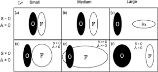
Figure 1 Schematic representation of the possible online (O, representing the “observations”) and offline forecast (F) combinations of the different components for the quantitative object-based metric SAL: structure (S), amplitude (A), and location (L). Modified from Wernli et al. (2008).

The S (Eq. 1) component in SAL captures information about the size and shape of ACL objects (Wilkins et al., 2016) by computing the normalized weighted mean mass difference (V, Eq. 2) for the online and offline forecasts:

$$\begin{array}{}\text{(1)}& {\displaystyle }S={\displaystyle \frac{V_{\mathrm{off}}-V_{\mathrm{on}}}{\mathrm{0.5}\left|V_{\mathrm{off}}+\left.V_{\mathrm{on}}\right|\right.}}.\end{array}$$

Weighted means (V) of the ash load fields in the column are estimated considering the total mass (R_n) and the scaled mass (V_n, Eq. 3) for the number of objects in the domain (M):

$$\begin{array}{}\text{(2)}& {\displaystyle }V={\displaystyle \frac{\sum _{n=\mathrm{1}}^M{R}_n{V}_n}{\sum _{n=\mathrm{1}}^M{R}_n}}.\end{array}$$

Scaled masses (V_n) for all objects are calculated separately for each object as follows:

$$\begin{array}{}\text{(3)}& {\displaystyle }{V}_n=\sum _{\left(xy\right)\in O_n}{R}_{xy}/R_n^{max},\end{array}$$

where xy is the grid cell location within the forecasted field, R_xy is the area-integrated concentration field (i.e., ash column mass in grams per square meter) in grid cell xy, and $R_n^{max}$ is the maximum grid cell ash mass in object O_n. Note that, in the case of a single object, V=V_n. Structure scores range between [$-\mathrm{2},\mathrm{2}$], with positive values indicating more objects in the offline forecast and that ACL values are too spread out and/or flat. A negative S score occurs when the offline forecast ACL objects cover too small of an area or are too peaked (or a combination of both).

The A component corresponds to the normalized difference of the domain-average ash mass values (R). This provides a simple measure of the quantitative accuracy of the total concentration of ash in the domain, ignoring the field's subregional structure:

$$\begin{array}{}\text{(4)}& {\displaystyle }A={\displaystyle \frac{{\overline{R}}_{\mathrm{off}}-{\overline{R}}_{\mathrm{on}}}{\mathrm{0.5}\left|{\overline{R}}_{\mathrm{off}}+\left.{\overline{R}}_{\mathrm{on}}\right|\right.}},\end{array}$$

where ${\overline{R}}_{\mathrm{off}}$ and ${\overline{R}}_{\mathrm{on}}$ are the ash masses averaged over all grid cells in the domain, i.e., ${\overline{R}}_n=\sum _{\left(xy\right)\in \mathrm{Domain}}{R}_{xy}/\phantom{R_{xy}\mathrm{domain}\mathrm{area}}\mathrm{domain}\mathrm{area}$. Amplitude scores range between [$-\mathrm{2},\mathrm{2}$], with 0 denoting no difference between offline and online forecasts. An amplitude score of +1 or −1 indicates that offline forecasts overestimate or underestimate, respectively, the domain-averaged ACL by a factor of 3. Scores of A=0.4 and 0.67 correspond to factors of 1.5 and 2, respectively (Wernli et al., 2008).

The L component of SAL compares the mass distribution between forecasts. The L component is composed of two parts:

$$\begin{array}{}\text{(5)}& {\displaystyle }L=L_{\mathrm{1}}+L_{\mathrm{2}}.\end{array}$$

The first one (L₁, Eq. 6) compares the normalized distance between the center of mass (C) of the offline and online ACL fields over the maximum distance within the entire domain (d):

$$\begin{array}{}\text{(6)}& {\displaystyle }{L}_{\mathrm{1}}={\displaystyle \frac{\left|C_{\mathrm{off}}+\left.C_{\mathrm{on}}\right|\right.}{d}}.\end{array}$$

The values of L₁ are in the range of [0,1], with L₁=0 suggesting identical centers of mass for both forecasts. However, separated ash clouds could also have the same center of mass, and therefore L₁=0 would not necessarily indicate a perfect match. The second part of the location component (L₂, Eq. 7) aims to distinguish such situations by measuring the weighted average (H, Eq. 8) between the center of mass of the total ash load and the center of mass for each object (C_n):

$$\begin{array}{}\text{(7)}& {\displaystyle }& {\displaystyle }{L}_{\mathrm{2}}=\mathrm{2}\left[{\displaystyle \frac{\left|H_{\mathrm{off}}+\left.H_{\mathrm{on}}\right|\right.}{d}}\right]\text{(8)}& {\displaystyle }& {\displaystyle }H={\displaystyle \frac{\sum _{n=\mathrm{1}}^M{R}_n\left|C_{\mathrm{off}}+\left.C_{\mathrm{on}}\right|\right.}{\sum _{n=\mathrm{1}}^M{R}_n}}.\end{array}$$

In the event that both online and offline ACL fields have only one object, then L₂=0. A factor of 2 is used to scale L₂ to the range of L₁. Hence, the total location component of L can reach values between [0,2] and can only be possible for an offline forecast in which both the distance between objects and the center of mass agree with the online forecast. It is important to mention that since both offline and online computational domains are the same, the magnitude dependency of L on the size of the domain does not affect our interpretation of this SAL component.

Absolute SAL scores range from 0 to 6, with scores closest to 0 denoting the best agreement between forecasts. The computation of the structure and location components of SAL groups accounts for objects (i.e., adjacent grid cells) with a value above a given threshold for the forecasted variable. For this study, objects are given as $O_n,n=\mathrm{1},\mathrm{\dots },M$, where M is the number of objects in the model domain. Each object combines at least two grid cells to avoid unrealistic single ash-containing grid cells. As defined previously, the object identification threshold for the ACL is set to 0.2 g m⁻². Modeled ACL values below this threshold are omitted from all components of SAL.

2.3.2 Categorical evaluation scores

Table 1 Contingency table of binary events for categorical verification scores at each grid point.

From an operational perspective, it is also important to know whether the presence of volcanic ash constitutes an airspace threat or not. In that context, the significance of quantitative volcanic ash forecasts can be measured in terms of categorical evaluation scores (Jolliffe and Stephenson, 2012). These scores are less sensitive to larger errors than quantitative evaluation scores. This is particularly important for extremely skewed data such as ACL, providing the degree to which the forecast supports a decision maker during an emergency event (i.e., closure of airspace). Consequently, ash loads can be viewed categorically (or binary for “yes” or “no” events) according to whether that value exceeds a threshold (event) or not (non-event). Here, we compute a series of categorical evaluation scores based on a contingency table (Table 1), which describes the combined distribution of forecast events and non-events for each coupling strategy. In Table 1, “hits” represents the number of grid points for which both forecasts (offline and online) exceed the threshold previously established (0.2 g m⁻²); “misses” represents the number of points for which only online forecasts exceed this threshold; “false alarms” indicates the number of points for which only offline forecasts exceeded the threshold; and finally, “correct negatives” represents the number of points for which neither offline nor online forecasts exceeded the threshold value. In this paper, we use these binary skill metrics to calculate four categorical evaluation scores:

• a.

  Probability of detection (POD) measures the fraction of ash points observed in the online forecast and that were correctly predicted for the offline forecast. This score is good for rare events, should be used together with the FAR score (FAR, Eq. 10), and is insensitive to false alarms. The POD score can reach values between [0,1]:

  $$\begin{array}{}\text{(9)}& {\displaystyle }\mathrm{POD}={\displaystyle \frac{\mathrm{hits}}{(\mathrm{hits}+\mathrm{misses})}};[\mathrm{0},\mathrm{1}].\end{array}$$
• b.

  False alarm ratio (FAR) measures the fraction of ash points predicted by the offline forecast that were observed to be non-events (i.e., not exceeding the threshold) in the online forecast. This score should be used together with the previous POD score and ignores the misses. The FAR score can reach values between [0,1]:

  $$\begin{array}{}\text{(10)}& {\displaystyle }\mathrm{FAR}={\displaystyle \frac{\mathrm{false}\mathrm{alarm}}{(\mathrm{hits}+\mathrm{false}\mathrm{alarm})}};[\mathrm{0},\mathrm{1}].\end{array}$$
• c.

  Frequency bias (FBI) measures the ratio of frequency of offline forecast points to the frequency of observed ash points in the online forecast. This score indicates whether the forecast system has a tendency to underestimate (FBI < 1) or overestimate (FBI > 1) events. However, it does not measure how well the offline forecast corresponds to the online simulation and only measures relative frequencies. The FBI score can reach values between [0,∞]:

  $$\begin{array}{}\text{(11)}& {\displaystyle }\mathrm{FBI}={\displaystyle \frac{\left(\mathrm{hits}+\mathrm{false}\mathrm{alarm}\right)}{(\mathrm{hits}+\mathrm{misses})}};[\mathrm{0},\mathrm{\infty }].\end{array}$$
• d.

  Critical success rate (CSI) measures the fraction of all offline and online forecast points that were correctly diagnosed and does consider both misses and false alarms. The CSI score can reach values between [0,1]:

  $$\begin{array}{}\text{(12)}& {\displaystyle }\mathrm{CSI}={\displaystyle \frac{\mathrm{hits}}{(\mathrm{hits}+\mathrm{misses}+\mathrm{false}\mathrm{alarms})}};[\mathrm{0},\mathrm{1}].\end{array}$$

  Similar metrics, such as the Figure of Merit in Space (FMS; Galmarini et al., 2010), have been used in previous works (e.g., Wilkins et al., 2016) to complement the SAL score for the evaluation of the spatial coverage between forecasts:

  $$\begin{array}{}\text{(13)}& {\displaystyle }\mathrm{FMS}={\displaystyle \frac{B_{\mathrm{off}}\cap B_{\mathrm{on}}}{B_{\mathrm{off}}\cup B_{\mathrm{on}}}};[\mathrm{0},\mathrm{1}],\end{array}$$

  where B_off and B_on are the modeled and observed ACL areas, respectively. In both cases, a score of 1 suggests a complete spatial overlap of the evaluated forecast. Alternatively, the spatial overlap will decrease as these scores reach values close to 0. Here, we employ the FMS metric to evaluate the spatial coverage of the forecasts and to complement a missing spatial coverage component in SAL. To be consistent with our implementation of SAL, the spatial ash coverage is computed only for forecast ACL fields exceeding a threshold of 0.2 g m⁻². However, it is worth mentioning that a low FMS score could also suggest two similar shapes shifted in space (Mosca et al., 1998) and, therefore, should be used together with the SAL score.

3 Synthetic case study

The first step of our evaluation consists of isolating the model's shortcomings and systematic errors that are exclusively associated with the offline coupling strategy employed in traditional volcanic ash forecasts. To this purpose, we constructed a preliminary synthetic case based on the first 48 h of the 2011 Caulle eruption with constant ESPs. This synthetic application reduces the differences associated with the source term (i.e., different source term quantification because of different wind fields) and allows us to isolate the systematic errors coming from the offline coupling approach. Within this framework, we limited the eruption duration to 12 h, using a constant column height and employing the Mastin et al. (2009) relationship (mass eruption rate vs. column height) for the dispersion evaluation of a single bin of ash (one particle class) during the first 48 h of the event. Multiple regional simulations of NMMB-MONARCH-ASH were performed to produce four different offline coupled forecasts, in which meteorological variables are updated at the specified coupling intervals (i.e., 1, 3, 6, and 12 h). Details about the 2011 Caulle eruption, accompanying meteorological conditions and the computational domain, are described in Sect. 4.2. Table 2 provides a summary of the ESPs used for this application. The skills of these forecasts were compared against the online coupled simulation, employing the quantitative and categorical evaluation scores described in Sect. 2.3. Scores at the end of the simulation (48 h) are shown in Table 3. For the purpose of this paper, we focus on describing the scores for the 3 and 6 h offline coupled forecasts, representative of an operational forecast driven by a global MetM.

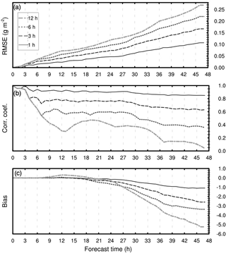
Figure 2 Quantitative evaluation scores for NMMB-MONARCH-ASH synthetic application: (a) root mean square error; (b) Pearson's correlation coefficient; (c) error bias.

Figure 2 shows the results of the quantitative evaluation scores, RMSE (Fig. 2a), correlation coefficient (Fig. 2b), and bias (Fig. 2c), as a function of the forecast's length for each coupling interval in the synthetic case. These scores assist in determining the degree to which offline forecasts correspond to the best estimate of the true outcome (online forecast). In general terms, and as expected a priori, all scores indicate that the quality of the forecast decreases with longer coupling intervals (i.e., 1, 3, 6, and 12 h) and length of the forecast. The RMSE score is presented in Fig. 2a and is used to assess the average magnitude of the offline forecast errors. Figure 2b shows how the linear association between the online and offline forecasts (Pearson's correlation coefficient) significantly decreases with longer coupling intervals, reaching noticeably low correlations. For example, for a 3 h coupled (i.e., meteorological data coupled in intervals of every 3 h) forecast the resulting coefficient after 24 h of simulation is below 0.6, while for a 6 h coupled forecast (coupled in intervals of every 6 h) it is below 0.5, and below 0.4 after 48 h. These scores indicate that traditional offline forecasts are not capable of reproducing more than half of the true outcome, suggesting that the coupling frequency in tephra dispersal modeling could be a critical source of error. This result is relevant considering that most emergency model setups employ 3 h temporal resolution forecasts with update frequencies of 6 h or more (Bowman et al., 2013; WMO, 2012). Finally, Fig. 2c depicts the forecast bias over that from the online simulation. In general terms, all offline forecasts underestimate ACL, reaching values between −1 and −5 g m² at the end of the forecast for the 1 and 12 h coupling intervals, respectively (Table 3).

Table 2 Summary of eruption source parameters (ESPs) used in NMMB-MONARCH-ASH for the synthetic case and the 2010 Eyjafjallajökull and 2011 Cordón Caulle applications.

Table 3 Evaluation scores for the synthetic case at the end of the 48 h forecast with NMMB-MONARCH-ASH. Metrics: Pearson's correlation coefficient (R); root mean square error (RMSE); error bias (BiAS); structure (S); amplitude (A); location (L); absolute SAL (| SAL |); probability of detection (POD); false alarm ratio (FAR); frequency bias (FBI); and Figure of Merit in Space (FMS).

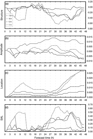
Figure 3 SAL evaluation scores for NMMB-MONARCH-ASH synthetic case: (a) structure; (b) amplitude; (c) location; (d) combined SAL.

Figure 3 illustrates the results from the quantitative object-based metric SAL, aimed at evaluating the variation in space and time of the forecasts. As with previous scores, the error associated with the SAL score also increases with the length of the coupling frequency. For all offline simulations within the synthetic case, the structure component of the metric (Fig. 3a) explains most of the discrepancy with the online forecast. Negative values of S indicate that offline forecasts predict fields that cover too small of an area and/or are too peaked. In addition, results from the amplitude and location components indicate a slight underestimation of the domain-averaged ACL for most offline forecasts, employing comparable centers of mass with the online reference. In general terms, systematic differences in the offline forecast are 3 and 5 times higher for a coupling frequency of 3 and 6 h than those of the 1 h interval (Table 3).

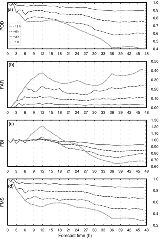
Figure 4 Categorical evaluation scores for the NMMB-MONARCH-ASH synthetic case including (a) probability of detection (POD), (b) false alarm ratio (FAR), (c) frequency bias (FBI), and (d) Figure of Merit in Space (FMS).

Categorical scores resulting from the evaluation of the synthetic case are summarized in Fig. 4. As in the previous scores, a threshold value of 0.2 g m⁻² is considered to define the ash-contaminated objects, categorizing these as yes or no events depending on if they exceed the threshold or not. These scores are critical for the aviation industry during a volcanic crisis since they can determine the closure of the airspace or the cancellation of flights. Figure 4a illustrates the POD for each forecast. As expected, this metric clearly shows how the probability of detecting ash-contaminated points in the offline forecasts decreases with longer coupling intervals and the forecast length. In addition, this figure also suggests that POD scores decrease considerably during the first hours of the forecast, matching the time for which the source was active. This trend is applicable to all categorical evaluation scores. After 48 h, the POD scores for the 3 and 6 h coupled forecasts are 0.752 and 0.603, respectively. For coupling frequencies above 6 h, the probability of detecting ash-contaminated areas drops below 50 % (e.g., 12 h coupled forecast in Table 3). POD scores are complemented by the results from the FAR metric, which measures the fraction of ash events predicted by the offline forecasts that were observed to be non-events. FAR scores (Fig. 4b) are consistent with POD scores, predicting 25 % of false ash-contaminated objects after 48 h of simulation (6 h coupled forecast). The equivalent plot for the FBI metric as a function of forecast length is shown in Fig. 4c. This metric indicates that all forecasts tend to underestimate the ACL, especially while the eruption is active. After that time, FBI scores stabilize between values ranging from 0.7 to 1.0. Finally, Fig. 4d illustrates the spatial overlap between offline and online forecasts defined by the FMS. This metric provides similar results to the POD metric. However, in this case, false alarms (Table 1) are also considered in the metric, leading to FMS scores lower than those for the POD metric. Considering this, FMS scores indicate that the spatial overlap (i.e., probability of hits over hits, misses, and false alarms) between the online and the 3 h coupled offline forecast after 48 h of simulation is around 65 % and below 50 % for the 6 h coupled forecast (Table 3).

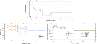
Figure 5 Eruption source parameters for the 2010 Eyjafjallajökull application: (a) column height fluctuation over time; (b) resulting MER over time considering different plume parameterizations (FPLUME – Folch et al., 2016; Woodhouse – Woodhouse et al., 2013; Mastin – Mastin et al., 2009; Degruyter – Degruyter and Bonadonna, 2012); (c) resulting MER for each coupling strategy (meteorology coupled online or with intervals of time of 1, 3, 6, and 12 h) with the Degruyter option only.

4 Application examples

In addition to the synthetic case, we present two applications of NMMB-MONARCH-ASH for the simulation of the initial phases of the 2010 Eyjafjallajökull and 2011 Cordón Caulle eruptions. In these cases, offline forecasts are evaluated taking into account the effects of the coupling interval and the actual changes in the ESPs (i.e., mass eruption rate (MER) depending on wind field) for each event. A summary of the ESPs used for each application is presented in Table 2. These two events have shed light on the importance of ash dispersal in the context of aviation safety (Bonadonna et al., 2012), and they suitably illustrate the severe disruptive effects of European and South American eruptions. Similar to the synthetic case, online and offline forecasts were compared on the same temporal scales and spatial grid; a gridded (point-to-point) evaluation was performed between forecasts following the criteria presented in the contingency Table 1; the output of the online forecast was considered as the “observed” (best estimation of true outcome) field; and a threshold of 0.2 g m⁻² was employed as the ACL detection limit.

For each application we include (i) a brief description of the eruptive event; (ii) a summary of the modeling setup to simulate the eruption; and (iii) a comprehensive evaluation of the plume dispersal forecast including qualitative, quantitative, and categorical evaluations and metrics. For the purpose of summarizing the results of these evaluation scores, we focus on describing those scores from the 6 h coupled forecast.

4.1 The 2010 Eyjafjallajökull eruption

The April 2010 eruption of Eyjafjallajökull volcano (63.6^∘ N, 19.6^∘ W, vent height 1666 m a.s.l.) in southern Iceland created unprecedented disruptions to European air traffic during 15–20 April. On 14 April a major outbreak of the central crater under the covering ice cap led to surface activity, causing phreatomagmatic explosions, generation of volcanic ash, and eruption columns rising up to 9 km (a.s.l) (Institute of Earth Sciences, 2010). The initial ash clouds traveled rapidly across the North Atlantic and North Sea, reaching southern Norway on 15 April and then traveling southwards as a frontal cloud crossing over to many northern European countries. In turn, the London VAAC dispatched immediate warnings to European aviation authorities and other VAAC centers every 3–6 h. The southern part of the ash cloud finally grounded in the northern part of the Alps. On 20 April new guidelines based on safe ash concentration thresholds were adopted, allowing for the ability to resume operations in large areas previously banned. In addition, several other ash cloud episodes occurred during late April and May, disrupting the European airspace for a total of 13 days (over 4 million passengers stranded due to cancellation or delay of over 100 000 flights), affecting 25 countries, and costing the aviation industry billions of euro (Oxford Economics, 2010). These impacts brought into focus how significantly volcanoes can affect communities and economies far away from the source and the critical importance of accurate volcanic ash forecasts.

4.1.1 Modeling setup

For the purpose of simulating this eruption, we employed NMMB-MONARCH-ASH with a model domain consisting of 401×428 grid points, covering the northern and western regions of Europe and using a grid with a horizontal resolution of 0.15^∘ × 0.15^∘ and 60 vertical layers. The top pressure of the model was set to 10 hPa (∼ 26 km) with a mesh refinement near the top (to capture the dispersion of ash) and the ground (to capture the characteristics of the atmospheric boundary layer). The computational domain spans in longitude from 30^∘ W to 30^∘ E and in latitude from 34^∘ S to 84^∘ N. The ESPs characterizing the event are described in Table 2 and presented in Fig. 5. Figure 5a shows the variations in column height for the duration of the forecast. Figure 5b illustrates the results from estimating the MER using the different formulations available in NMMB-MONARCH-ASH (Marti et al., 2017). Figure 5c shows the MER variations associated with the different offline coupling intervals with the MetM and compare them with the fully coupled online forecast.

4.1.2 Qualitative evaluation

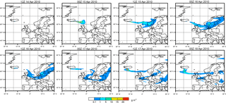
Figure 6 shows the plume dispersal (ash column loading; ACL) from the online forecast corresponding to the first explosive phase (14–18 April) of the Eyjafjallajökull eruption (Gudmundsson et al., 2012). This phase is conveniently divided into 14–16 April, when the volcanic plume produced a well-defined sector towards the east, and 17 to early 18 April, when northerly winds drove the plume to the south. Complementary to this figure, Fig. 7 illustrates the airspace contamination forecasted by the model during the first phase of the eruption at flight levels FL050 and FL200. This figure illustrates the ash hazard aviation guidelines, which distinguish zones of low (green, ash concentration less than 0.2 mg m⁻³), moderate (orange, ash concentration between 0.2 and 2 mg m⁻³), and high (red, ash concentration above 2 mg m⁻³) concentration of ash employed to regulate no-fly zones. This information is critical for air traffic management to assist flight dispatchers while planning flight paths and designing alternative routes in the presence of a volcanic eruption. Model results show the volcanic cloud traveling E-NE, achieving critical concentration values in northern Europe during 15–17 June, and suggesting severe disruptions in the European airspace.

Figure 6 NMMB-MONARCH-ASH total ACL (mass loading; g m⁻²) for the 2010 Eyjafjallajökull application.

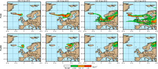
Figure 7 Ash hazard aviation guidelines applied for 2010 Eyjafjallajökull application over time. Zones of low (green, ash concentration < 0.2 mg m⁻³), moderate (orange, ash concentration between 0.2 and 2 mg m⁻³), and high (red, ash concentration above 2 mg m⁻³) concentration are displayed for FL50 (top) and FL200 (bottom).

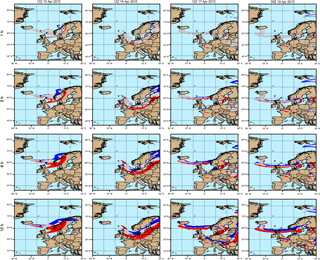
Figure 8 Qualitative comparison between the online and offline forecasts with 1 h (row 1), 3 h (row 2), 6 h (row 3), and 12 h (row 4) coupling intervals. Gridded evaluation is performed following the criteria presented in the contingency Table 1. Hit (grey), missed (red), and false alarm (blue) predictions are shown for the 2010 Eyjafjallajökull case over time.

Figure 8 shows a qualitative comparison between the online and the different offline coupled forecasts for Eyjafjallajökull application. Qualitative comparisons are presented for each coupling interval in different rows (i.e., first row: 1 h; second row: 3 h; third row: 6 h; fourth row: 12 h coupling). Areas in grey (hits) represent grid points for which both forecasts (offline and online) exceed the established threshold. Red areas (misses) indicate those regions where the offline forecast fails to predict existing ash (underprediction). Finally, blue areas (false alarms) illustrate those domain areas for which only offline forecasts exceed the threshold, implying a false prediction of ash (overprediction). In general terms, offline forecasts for the Eyjafjallajökull event tend to overpredict towards the north of the plume and to underpredict towards the south. While results of the 1 h offline forecast indicate mostly hits (H), Fig. 8 clearly suggests that the number of missed (M) and false alarm (FA) points increases with longer coupling intervals and the length of the forecast. This is due to the prevailing mid-troposphere south-oriented wind acceleration over the south of Iceland and the North Sea (Folch et al., 2012), and it is consistent with those results presented previously in the synthetic case. As a consequence, these forecasts would miss, for example, the arrival of volcanic ash over northern Germany in the late afternoon of 16 April as indicated by the Deutscher Wetterdienst (DWD) ceilometer network at the time of the eruption (Flentje et al., 2010). As a general approximation, Fig. 8 suggests that for the Eyjafjallajökull eruption, offline forecasts with coupling intervals of 3 h and above could result in significant inconsistent predictions (M + FA areas).

4.1.3 Quantitative and categorical evaluation

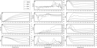
Figure 9 shows the results of the quantitative and categorical metrics for the ACL offline forecasts for the 2010 Eyjafjallajökull application. Complementing this figure, Table 4 shows the scores for all coupled forecasts after 48 h from the eruption starting time. As found in the synthetic case, quantitative and categorical metrics lessen their scores for longer coupling intervals and forecast lengths.

Figure 9 Online vs. offline evaluation scores for the 2010 Eyjafjallajökull case.

Table 4 Evaluation scores for the 2010 Eyjafjallajökull eruption application at the end of the 48 h forecast with NMMB-MONARCH-ASH. Metrics: Pearson's correlation coefficient (R), root mean square error (RMSE), error bias (BiAS), structure (S), amplitude (A), location (L), absolute SAL ($\left|\mathrm{SAL}\right|$), probability of detection (POD), false alarm ratio (FAR), frequency bias (FBI), and Figure of Merit in Space (FMS).

Quantitative evaluation scores RMSE (Fig. 9a), correlation coefficient (Fig. 9b), and bias (Fig. 9c) show more comparable trends than those reported for the synthetic case. After 48 h of simulation, the 3 h coupled forecast scores show barely any correlation with the online forecast and a RMSE of 0.122 g m⁻². Bias scores suggest that all offline forecasts tend to underestimate ACL between −0.33 and −2.5 g m² at the end of the forecast. Figure 9d–g illustrate the results from the quantitative object-based metric SAL, quantifying the variation in space and time of the forecasts. For the Eyjafjallajökull application, both the structure (Fig. 9d) and amplitude (Fig. 9e) from the offline forecasts explain most of the discrepancy with the online forecast. Contrary to the synthetic case, in which the A component had a residual effect towards the total SAL, in this application the offline forecasts tend to underestimate the amplitude component by 20 % for coupling intervals equal to or above 3 h. This is anticipated since meteorological conditions are updated at each given interval and no additional ash-contaminated objects are found in the domain. After the first coupling with the MetM takes place, scores start to stabilize. After this time, the A component stabilizes, reducing its associated underestimation factor. Location scores (Fig. 9f) suggest a comparable mass distribution of the ACL fields for the online and offline forecasts. Finally, absolute SAL scores after 48 h of simulations (Table 4) indicate that systematic differences in the offline forecast are approximately 2 times higher for a coupling frequency of 3 h than those of the 1 h interval.

Categorical scores for the Eyjafjallajökull application are summarized in Fig. 9h–k. Results from the POD metric (Fig. 9h) show that the probability of detecting ash-contaminated events in the offline forecasts decreases with longer coupling intervals, especially during the time the first coupling with the MetM occurs. After 48 h, the POD score for the 3 h coupled forecast is around 65 % and below 50 % (i.e., 0.46) for the 6 h coupled forecast. Conversely, results from the FAR metric follow an increasing trend (Fig. 9i), misrepresenting nearly 45 % objects in the domain. Results from the FBI metric (Fig. 9j) indicate that all offline forecasts tend to underestimate the ACL. Finally, FMS scores suggest that the spatial overlap between the online and the offline forecasts after 48 h of simulation is below 50 % for those simulations with coupling intervals of 3 h or more.

4.2 The 2011 Cordón Caulle eruption

The 2011 Cordón Caulle eruption exemplifies a typical mid-latitude Central and South Andean eruption. The Cordón Caulle volcanic complex (Chile, 40.5^∘ S, 72.2^∘ W, vent height 1420 m a.s.l.) reawakened on 4 June 2011 around 18:30 UTC after decades of quiescence. The initial explosive phase spanned over more than 2 weeks, generating ash clouds that dispersed over the Andes (Collini et al., 2013). The climatic phase (∼ 27 h) (Jay et al., 2014) was associated with a ∼ 9 km (a.s.l.) high column (Osores et al., 2014). For the period between 4 and 14 June, numerous flights and airports were disrupted in Paraguay, Uruguay, Chile, southern Argentina, and Brazil (Wilson et al., 2013).

4.2.1 Modeling setup

The model domain for this application consists of 268×268 grid points covering the northern regions of Chile and Argentina using a horizontal resolution of 0.15^∘ × 0.15^∘ and 60 vertical layers. The top pressure of the model was set to 10 hPa (∼ 26 km). The computational domain spans in longitude from 41 to 81^∘ W and in latitude from 18 to 58^∘ S. The ESPs characterizing the Caulle event are described in Table 2. Figure 10a shows the slight variation in column height for the duration of the forecast (Osores et al., 2014). Figure 10b illustrates the results from simulating the MER over time considering different coupling strategies.

Figure 10 Eruption source parameters for the 2011 Cordón Caulle case: (a) column height fluctuation over time. (b) Resulting MER over time for each coupling strategy (meteorology coupled online or with intervals of time of 1, 3, 6, and 12 h).

Figure 11 NMMB-MONARCH-ASH total column load (mass loading; g m⁻²) for the 2011 Cordón Caulle case.

4.2.2 Qualitative evaluation

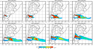
Figure 11 illustrates the plume dispersion from the online forecast associated with the early Plinian phase (4–7 June) of the Cordón Caulle eruption. The initial ash cloud reached the Atlantic coast on 4 June late afternoon (Collini et al., 2013), just before turning to the northeast to reach the northern part of Argentina during the 6 June and the city of Buenos Aires in the days after. The effect of the plume dispersion on air-traffic management is shown in Fig. 12. This figure shows the airspace contamination forecasted by the model during 4–6 June at flight levels FL050 and FL200. Model results show the volcanic cloud achieving critical concentration values within a wide area east of the Andes range. On 6 June, simulation results show the volcanic cloud moving east, threatening the main international airports that service the province of Buenos Aires. These results suggest that the cancellation of multiple flights in several Argentinean airports during this time was justified.

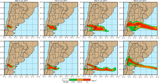
Figure 12 Ash hazard aviation guidelines applied for the 2011 Cordón Caulle application over time. Zones of low (green, ash concentration < 0.2 mg m⁻³), moderate (orange, ash concentration between 0.2 and 2 mg m⁻³), and high (red, ash concentration above 2 mg m⁻³) concentration are displayed for FL50 (top) and FL200 (bottom).

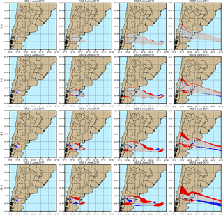
Figure 13 Qualitative offline vs. online forecast comparison for 1 h (row 1), 3 h (row 2), 6 h (row 3), and 12 h (row 4) coupling intervals. Gridded evaluation is performed following the criteria presented in the contingency Table 2. Hit (grey), missed (red), and false alarm (blue) predictions are shown for the 2011 Cordón Caulle application over time.

Figure 13 shows the qualitative comparison between the online and offline coupled forecasts for the first days of the 2011 Cordón Caulle eruption. In this case, given that the plume height during the first hours of the eruption was more consistent (no significant changes in wind speed and direction) than for the Eyjafjallajökull application, the difference between forecasts is less suggestive, although still remarkable. Contrary to the Eyjafjallajökull application, offline forecasts tended to underestimate to the north of the plume and slightly overestimate to the south. The resulting evaluation from these inconsistencies indicates that offline forecasting with longer coupling intervals missed the abrupt shift in the plume course known to be associated with early 6 June. This alteration was due to the change in the wind direction toward the N-NE first and then again towards the SE (e.g., Elissondo et al., 2016). As a consequence, these results suggest that offline forecasts would miss the correct arrival time of volcanic ash to the main international airports in Buenos Aires a few days later (i.e., Ezeiza and Aeroparque Jorge Newbery airports).

4.2.3 Quantitative and categorical evaluation

Figure 14 Online vs. offline evaluation scores for the 2011 Cordón Caulle application.

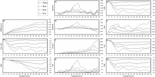
Figure 14 summarizes the results for the quantitative and categorical metrics for the 2011 Caulle application. Metric scores at the end of the simulation are presented in Table 5. Results for the Cordón Caulle application are consistent with those from the synthetic case and the Eyjafjallajökull application in that the uncertainty of the forecast increases significantly with the length of the coupling frequency employed. Quantitative evaluation scores RMSE (Fig. 14a), correlation coefficient (Fig. 14b), and bias (Fig. 14c) show comparable trends to those from the Eyjafjallajökull application. Despite this similarity, linear correlation coefficients between offline and online forecasts for the Caulle application are higher than those from the Eyjafjallajökull simulation. This result is explained by the fewer changes in the source term (e.g., variations in the column height) during the Caulle event. After 48 h of simulation, the 3 h coupled forecast scores a correlation coefficient of 0.80 with a RMSE of 0.11 g m⁻², while the 6 h coupled forecast scores 0.6 and 0.16 g m⁻², respectively. Bias scores suggest that all offline forecasts tend to underestimate ACL between −0.13 and −4.75 g m⁻² at the end of the forecast.

Table 5 Evaluation scores for the 2011 Cordón Caulle eruption application at the end of the 48 h forecast with NMMB-MONARCH-ASH. Metrics: Pearson's correlation coefficient (R), root mean square error (RMSE), error bias (BiAS), structure (S), amplitude (A), location (L), absolute SAL ($\left|\mathrm{SAL}\right|$), probability of detection (POD), false alarm ratio (FAR), frequency bias (FBI), and Figure of Merit in Space (FMS).

Figure 14d–g illustrate the results from the quantitative object-based metric SAL for the Cordón Caulle event. SAL scores (Fig. 14g) suggest that differences between online and offline strategies for the Cordón Caulle application are considerably higher than those for the Eyjafjallajökull application. This is due to the changing meteorological conditions during to the Cordón Caulle event and confirms that inconsistences associated with offline forecasts are more relevant in scenarios in which the meteorological conditions (mainly wind speed and direction) vary rapidly in time. In terms of the individual components of SAL, structure (Fig. 14d) and amplitude (Fig. 14e) scores explain most of the discrepancy with the online forecast. Structure scores indicate that more objects occur in the offline forecast and ACL values are too spread out and/or flat, while amplitude scores suggest that offline forecasts tend to underestimate the total concentration of ash in the domain up to 50 %. The systematic error associated with the offline forecasts is clearly demonstrated after 18 h of simulation (Fig. 14g), time during which changes in wind speed and direction start to be noteworthy (Fig. 11). Location scores (Fig. 14f) suggest a consistent mass distribution of the ACL fields amongst forecasts. The Cordón Caulle application is a perfect example to illustrate the importance of complementing traditional quantitative metrics with the quantitative object-based metric SAL. For this particular case, SAL scores are able to capture the inconsistences of the offline dispersion forecast due to the changing meteorological conditions that other quantitative metrics (i.e., RMSE, correlation coefficient, bias) cannot account for.

Finally, categorical scores for the Cordón Caulle application are presented in Fig. 14h–k. Results suggest that the skill of the forecast decreases with longer coupling intervals, following trends similar to those found in the Eyjafjallajökull application. After 48 h, FMS scores suggest that the spatial overlap between the online and the 6 h coupled offline forecasts is below 65 % and around 80 % for the 3 h coupled forecast (Table 5; Fig. 14k), with a probability of misrepresenting ash-contaminated objects by around 10 % (FAR; Fig. 14i). Results from the FBI metric (Fig. 14j) indicate that all offline forecasts tend to underestimate the ACL.

5 Discussion

Volcanic ash modeling systems are used to simulate the atmospheric dispersion of volcanic ash and to generate forecasts to quantify the impacts from volcanic eruptions on air quality, aviation, and climate. However, volcanic ash forecasts require the consideration of numerous and complex uncertainties. The 2010 Eyjafjallajökull eruption clearly demonstrated the need for a better understanding of the uncertainties associated with the dispersal model employed in operational volcanic ash forecasting. Since then, the scientific community has focused on identifying and improving uncertainties primarily associated with the characterization of the source term (e.g., MER, column height). However, and surprisingly, the quantification of systematic errors and shortcomings associated with the meteorological data driving the dispersion model has received little attention. Traditionally, operational volcanic ash forecasts employ offline coupling strategies to produce the required meteorological fields at regular time intervals, e.g., every 1 or 6 h for typical mesoscale and global operational MetM configurations, respectively. In previous sections of this paper, we have shown the meaningful negative impact of employing offline coupling intervals on the accuracy of the ash-cloud simulations as compared to online coupled forecasts. In particular, Sect. 3 showed the scores from evaluating a synthetic case focusing exclusively on the effect of the coupling approach. Evaluation scores reveal that the uncertainty of the offline forecasts increases significantly with the length at which the meteorological driver is coupled with the dispersion model (e.g., up to 4 times for the 6 h coupled forecast). However, the question of how this compares to other better-constrained sources of forecast error still remains unanswered.

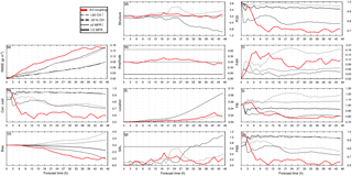
Figure 15 Online vs. offline evaluation scores for the NMMB-MONARCH-ASH synthetic application representing the uncertainty associated with the source term. ESPs were modified for the eruption column height (±20 %) and MER (×2 and 1∕2). Scores are compared with those from the 6 h offline coupled forecasts (red line).

This section aims to answer this question by evaluating to what extent the magnitude of the model forecast errors implicit in the offline approach compares with that of the source term. For this purpose, we performed four additional experimental simulations under the synthetic case in which ESP for the online forecast were modified by (i) employing a ±2 MER factor (i.e., ×2 and 1∕2 times the original MER) and (ii) varying the corresponding column height by ±20 %. As in previous applications, experimental forecasts were evaluated on the same temporal scales and spatial grid against the online forecast employing a range of complementary quantitative and categorical metrics. Figure 15 illustrates the evaluation scores from these four simulations and compares them with those of the 6 h coupled offline forecast. Overall, Fig. 15 reveals that systematic errors and shortcomings associated with the traditional offline coupling strategies employed in operational volcanic ash forecast are of the same order of magnitude as those uncertainties attributed to the characterization of the source term. For example, correlation coefficients (Fig. 15b) and POD scores (Fig. 15h) suggest an additional 10–30 % level of uncertainty attributed to the 6 h coupled forecast than those associated with the source term. In that same context, at the end of the simulation, FMS scores (Fig. 15k) reveal that the spatial overlap between the online and the 6 h coupled offline forecasts is ∼ 20 % lower than that from varying the column height by ±20 %, and ∼ 50 % lower than those from altering the original MER.

These results suppose a significant advance in the quantification of the uncertainty sources associated with traditional offline volcanic ash forecasts.

6 Conclusions

This paper quantifies the systematic errors inherent in offline coupling strategies employed for operational volcanic ash forecasting. For this purpose, we employed the different coupling strategies available in the NMMB-MONARCH-ASH model to evaluate the predictability limitations of the offline forecast against the online forecast. Model comparisons were performed for a synthetic case study focusing exclusively on the effect of the coupling approach, and for two historical cases accounting for changing meteorological conditions and ESPs. Evaluation scores indicate that systematic errors credited by offline forecast are of the same order of magnitude as those better-constrained uncertainties associated with the source term. In particular, offline forecasts in operational setups can result in significant errors in the dispersion of the ash plume for coupling intervals above 3 h. The results of this study show that 3 h coupling offline forecasts fail to reproduce about 35 % of the online forecast (best estimate of the true outcome) for a case with constant ESPs (synthetic case): close to 50 % for the 2010 Eyjafjallajökull case and 20 % for the 2011 Cordón Caulle case. For offline forecasts with coupling intervals above 3 h, these discrepancies are significantly higher. These inconsistencies are anticipated to be even more relevant in scenarios in which the meteorological conditions change rapidly in time. The outcome of this paper advocates that operational groups responsible for real-time advisories for aviation consider employing computationally efficient online dispersal models.