the Creative Commons Attribution 4.0 License.
the Creative Commons Attribution 4.0 License.
 | 23 Feb 2018
Impact of biomass burning on pollutant surface concentrations in megacities of the Gulf of Guinea
Cyrille Flamant
Solène Turquety
Adrien Deroubaix
Patrick Chazette
Rémi Meynadier
In the framework of the Dynamics–Aerosol–Chemistry–Cloud Interactions in West Africa (DACCIWA) project, the tropospheric chemical composition in large cities along the Gulf of Guinea is studied using the Weather and Research Forecast and CHIMERE regional models. Simulations are performed for the May–July 2014 period, without and with biomass burning emissions. Model results are compared to satellite data and surface measurements. Using numerical tracer release experiments, it is shown that the biomass burning emissions in Central Africa are impacting the surface aerosol and gaseous species concentrations in Gulf of Guinea cities such as Lagos (Nigeria) and Abidjan (Ivory Coast). Depending on the altitude of the injection of these emissions, the pollutants follow different pathways: directly along the coast or over land towards the Sahel before being vertically mixed in the convective boundary layer and transported to the south-west and over the cities. In July 2014, the maximum increase in surface concentrations due to fires in Central Africa is ≈ 150 µg m−3 for CO, ≈ 10 to 20 µg m−3 for O3 and ≈ 5 µg m−3 for PM10. The analysis of the PM10 chemical composition shows that this increase is mainly related to an increase in particulate primary and organic matter.
- Article
(9885 KB) - Full-text XML
- BibTeX
- EndNote


The concentrations of gases and particles are rapidly growing in southern West Africa (SWA) and driven by the constant increase in anthropogenic atmospheric emissions. These emissions are linked with car traffic, industries, and related gas and oil extraction activities, domestic fires, and waste burning (Marais and Wiedinmyer, 2016). They are proportional to the population, which is increasing dramatically in urbanized areas (Adon et al., 2016). The atmospheric pollution problems are mainly present along the coast of the Gulf of Guinea spanning from Abidjan (Ivory Coast) to Port Harcourt (Nigeria) and occur in the lower few hundred metres above the surface in the atmospheric boundary layer (ABL). In addition to this anthropogenic regional pollution, the region is impacted by other important sources, especially in the summer, with large emissions of mineral dust from the Sahara and the Sahel to the north and vegetation fires from Central and southern Africa (Real et al., 2010). In the coastal region of SWA mineral dust and biomass burning aerosols are generally observed above the ABL, between 800 and 600 hPa, as the result of long-range transport. Mineral dust is transported from the north in the Saharan air layer (Parker et al., 2005) (Flamant et al., 2009) and can be mixed downward into the ABL over the Sudanian region (Crumeyrolle et al., 2011). Using a Lagrangian model, Mari et al. (2008) show that the intrusion of Southern Hemispheric biomass burning aerosol plumes occurred in the mid-troposphere over the Gulf of Guinea, but did not investigate whether these plumes could impact air quality over urbanized areas of SWA.
The variability of the atmospheric composition and its impact on West African climate and on the health of populations and ecosystems is the purpose of the Dynamics–Aerosol–Chemistry–Cloud Interactions in West Africa (DACCIWA) project (Knippertz et al., 2015). In this study, we concentrate on the summer of 2014, which was the focus of one of the dry run exercises conducted in preparation for the field campaign that took place in June–July 2016 (Flamant et al., 2018). The period corresponds to the onset of the West African Monsoon (WAM) when the rainy convective systems migrate from the coastal area along the Gulf of Guinea to the Sahel (Williams et al., 2010). The months of June and July 2014 were more prone to precipitation at the SWA coast than 2015 and 2016 due to a late monsoon onset. The precipitation and the dynamics associated with the related mesoscale convective systems strongly impact the vertical distribution of pollutants in the region and can contribute to improving or degrading air quality.
The goal of this study is to quantify the relative contribution of the pollutants associated with biomass burning from Central Africa on the surface concentrations of aerosols, carbon monoxide (CO), and ozone (O3) in urbanized areas pertaining to the DACCIWA project. In order to take into account all important sources, a large area is modelled encompassing SWA (Ivory Coast, Ghana, Togo, Benin, Nigeria) and representing all sites of interest for the DACCIWA project. We assess the relative contribution of vegetation biomass burning by investigating the difference between two simulations: one with and one without biomass burning emissions, from now on referred to as the FIRE and NoFIRE simulations, respectively. The chemical composition of the aerosols over coastal SWA is also presented.
Section 2 presents the observation locations. Section 3 presents the models and the specific configuration and changes developed for this study as well as a tracer release experiment. Section 4 presents an analysis of the long-range transport of gas and aerosol species and Sect. 5 an analysis of gas and aerosol surface concentrations in the cities located in the coastal areas. Conclusions are finally presented in Sect. 6.
Data from very different sources were used to conduct this study. They were obtained from space-borne platforms and ground-based stations. Satellite data provide information on the horizontal and vertical distributions and therefore on the long-range transport. Other measurements are available at specific locations, such as the aerosol optical depth (AOD) and surface concentrations of particulate matter with a diameter less than 10 µm (PM10). If the AOD measurements may be relative to any kind of aerosol source, the PM10 values are here related to measurements taken close to mineral dust sources only and are thus presented in the Appendix. Also note that for chemistry, there is a lack of in situ surface measurements for this region and during the studied period.
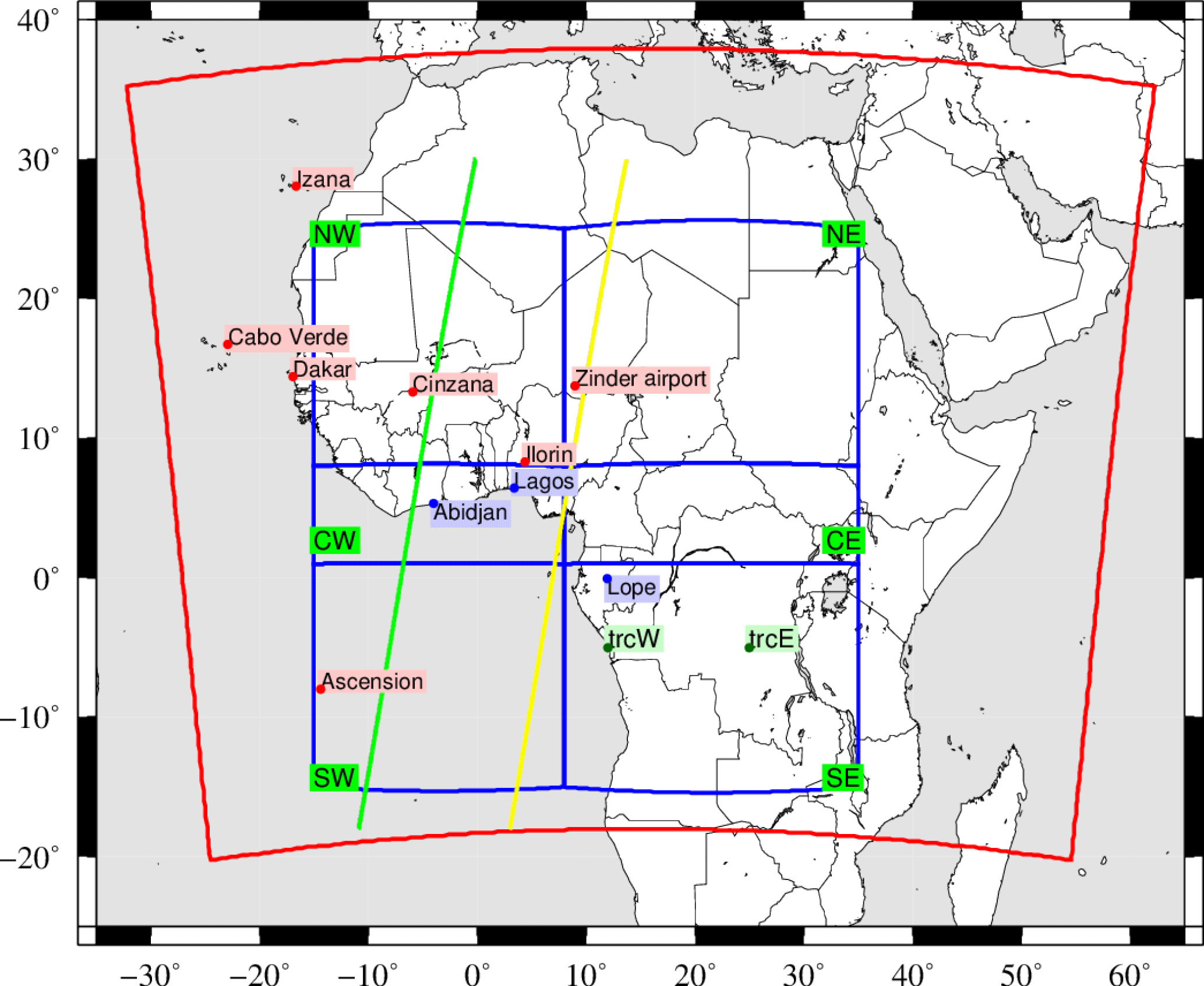
Figure 1Map of the modelled domain (the red frame). The circles and the location names indicate the stations described in Table 1: the red symbols represent the AERONET stations and the blue symbols represent locations representative of the most studied sites in the DACCIWA project. The two lines represent the CALIOP trajectories, with the green one for 26 July 2014 and the yellow one for 27 July 2014. The sub-domains defined for the comparisons between the model and the IASI data are in blue.
2.1 The AERONET data
The modelled aerosol optical properties are compared to observations using level 2 AERONET (AErosol RObotic NETwork; Holben et al., 2001) photometer data, namely (i) AOD at a wavelength of λ=550 nm and (ii) the Ångström coefficient calculated using the AOD measured at λ=470 and 870 nm. The stations used for the model validation are listed in Table 1 and their location is shown in Fig. 1. Note that, except for Lope, most of the AERONET stations are located in the northern part of the studied region, mainly under the influence of mineral dust emissions. Comparisons are performed using statistical scores calculated with an hourly time step and are presented for a given AERONET station only if data are acquired on a regular basis over a period of 3 months (i.e. 2280 h) and if more than 30 values can be used to compute them (only scores for which at least 1.5 % of data are available are shown).
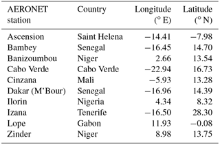
Table 1AERONET measurement stations with their names, countries, and coordinates (sorted by alphabetical order).
2.2 The satellite data
Three different satellite datasets are used in this study: (i) the Moderate Resolution Imaging Spectroradiometer (MODIS) for AOD, (ii) the Infrared Atmospheric Sounding Interferometer (IASI) for CO, and (iii) the Cloud-Aerosol Lidar with Orthogonal Polarization (CALIOP) for aerosol classification. The first two correspond to vertically integrated data when CALIOP provides vertical profiles.
The MODIS AOD product at 550 nm (from the MODIS–Terra aerosol 5 min L2 swath 10 km data collection 5.2) is used to quantify the increase in aerosol due to biomass burning (Levy et al., 2010). The model outputs and observations are collocated in space and time in order to exactly compare the model to the available observations.
The IASI CO total column retrievals by the FORLI algorithm (Clerbaux et al., 2009; George et al., 2009; Hurtmans et al., 2012) are used. CO is a product of incomplete combustion with a lifetime of several weeks. It can be used here as a tracer of biomass burning long-range transport. These observations are thus used to check if biomass burning aerosol plumes in the model are realistically represented and transported. The comparison between the model and the IASI observations consists of 3-day-averaged column-integrated CO concentrations. The model outputs are collocated in space and time with the satellite observations when they are available. They are also vertically corrected using the satellite averaging kernels before the vertical integration. For comparison to the model results, six sub-domains are defined to represent several regions as follows.
-
SW: the South-West domain is the only region entirely over the sea and may be under the plume of biomass burning aerosols coming from Central Africa.
-
SE: the South-East domain represents the region in Central Africa where vegetation fires are observed.
-
CW: the Central-West domain is the region containing the Gulf of Guinea cities studied in this article.
-
CE: the Central-East domain may be under the plume of vegetation fires coming from the South-East.
-
NW and NE: the North-West and North-East domains correspond to regions without vegetation fire emissions but with mineral dust emissions.
The CALIOP lidar measurements, on-board the Cloud-Aerosol Lidar Pathfinder Satellite Observation (CALIPSO) satellite (Winker et al., 2010), are analysed to obtain an aerosol sub-type classification (CALIOP v4.10 product), as proposed in Omar et al. (2010) and Burton et al. (2015). In addition, the product provides information on the vertical extent of aerosol layers as shown by Chazette and Royer (2017). The aerosol sub-type classification is built on thresholds of lidar-derived optical characteristics and is not error free, as mentioned by Burton et al. (2013) and Huang et al. (2015). Limitations associated with this aerosol classification are described in Tesche et al. (2013). A specific development was carried out for the comparison between CALIOP and the model results. It is described in detail in Appendix B.
For the simulations performed in this study, two regional models are used: (i) the Weather and Research Forecasting (WRF) model calculates the meteorological variables, and (ii) the CHIMERE chemistry-transport model calculates the concentrations of the tracers and the gaseous and aerosols species. WRF first calculates meteorological fields. Second, CHIMERE uses the meteorology from WRF and surface emission cadastres to simulate the chemical concentrations in the atmosphere. WRF and CHIMERE use the same horizontal domain and the same grid size of 60 km × 60 km.
The modelled period ranges from 1 May to 31 July 2014. The domain size is presented in Fig. 1. The model parameterizations and characteristics are detailed in Appendix A. A comparison between the WRF model results and meteorological measurements is presented in Appendix C.
In this section, we describe the tracer experiment and a dedicated development in the model pertaining to the vertical profile of biomass burning emissions.
3.1 The tracer experiment
The tracer release experiments are aimed at addressing the following question: what are the regions of Central Africa for which biomass burning aerosols can reach the coastal cities of the Gulf of Guinea?
The passive tracers are released from two locations in the western and eastern part of the biomass burning area in Central Africa for May–July 2014: trcW in Gabon at 12∘ E and −5∘ N, and trcE in the Democratic Republic of Congo at 25∘ E and −5∘ N (see Fig. 1). The corresponding experiments are named “trcW” and “trcE”. For each location, two vertical profiles of injection are used: experiments for which aerosols are injected between the surface and 3000 m a.g.l. are labelled “1” and experiments for which aerosols are injected from 3000 to 6000 m a.g.l. are tagged “2”. These two altitude intervals enable the estimation of the sensitivity of the biomass burning transport to different regimes of the injection height (Hp) values. The tracers behave as aerosols, with a density and a size distribution, and are thus subject to deposition during transport. The tracers are continuously released from 15 June to 30 July. There is no diurnal cycle, with the emissions flux being constant during the whole period. The released amount is arbitrary and has no unit (but for realism, the emitted fluxes are of the same order of magnitude as anthropogenic emissions in SWA).
3.2 The vertical profile of biomass burning aerosol emissions
The fires in Central Africa generally start in April and peak in July (Barbosa et al., 1999; Cooke et al., 1996). A lot of parameters are involved in the calculation of these emissions, making the wildfire fluxes one of the most uncertain sources in chemistry-transport models (Grell and Baklanov, 2011; Turquety et al., 2014). This flux calculation may be divided into three parts: (i) the emissions fluxes, (ii) the injection height Hp, and (iii) the shape of the injection height profile. The first two items have already been developed in CHIMERE and are now considered as validated schemes. They are detailed in Appendix D.
For this study, a specific development has been carried out on the shape of the vertical injection profile. This quantity is difficult to estimate but is often considered as a very sensitive parameter because the way emitted particles are vertically distributed in the lower troposphere will likely impact the long-range transport of biomass burning aerosols.
A lot of global models simply inject the emitted mass in an homogeneous way in the boundary layer or from the surface to a prescribed height Hp (see references in Sofiev et al., 2012, among others). Sofiev et al. (2013) distribute the flux homogeneously between Hp∕3 and Hp. Other models use more complex parameterizations based on thermal convective approaches primarily developed for boundary layer convection in dynamical models and adapted to the specific problematic of pyroconvection (Freitas et al., 2007; Rio et al., 2010). However, this “thermal” approach is numerically cost consuming and difficult to use, being very sensitive to the chosen input parameters. Finally, some vertical profiles are close to the vertical diffusivity profile (Kz) shape with the maximum of injection at the height Hp∕2, such as in Raffuse et al. (2012) and Veira et al. (2015).
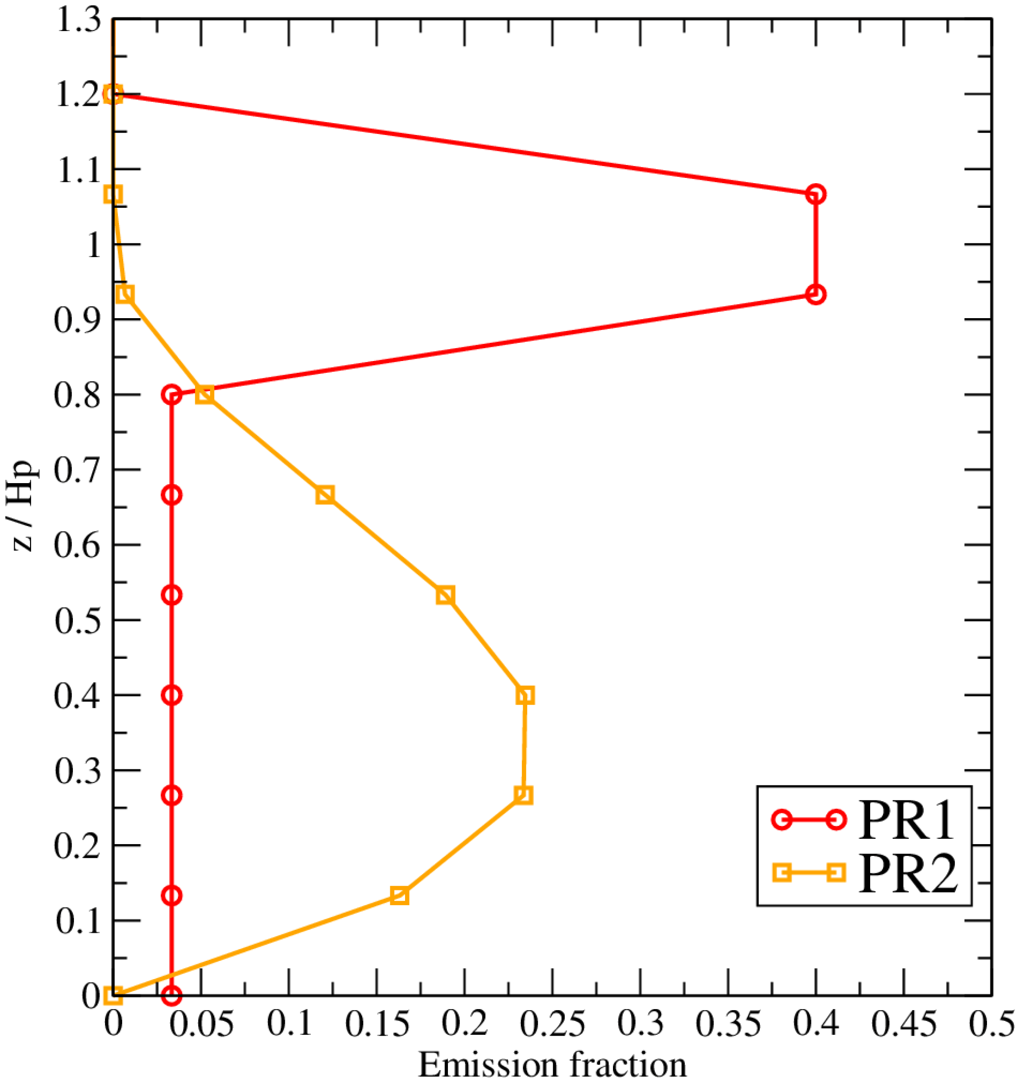
Figure 2Vertical profiles of factors used for the injection of biomass burning emissions in the troposphere.
In this study, and in order to reduce the uncertainty of our results, three simulations are performed.
-
NoFIRE. This simulation takes into account all processes (dynamic and chemistry) available in the CHIMERE model. All emissions are taken into account except the biomass burning emissions.
-
FIRE PR1 and FIRE PR2. These simulations have the same configuration as the NoFIRE simulation except that we add the biomass burning emissions fluxes. These emissions fluxes are injected in the troposphere following the two injection height profiles PR1 and PR2, which are described in Fig. 2. The difference FIRE–NoFIRE provides a quantification of the impact of biomass burning on the gas and aerosol atmospheric concentrations.
The differences between the PR1 and PR2 injection profiles are as follows.
-
PR1: 80 % of emissions are injected in the model layers included in the interval . The rest, 20 %, are injected between the surface and 0.9×Hp. This profile was selected to (i) estimate the long-range transport of biomass burning plumes and (ii) determine whether fires mainly injected in the mid-troposphere may have an impact on remote surface concentrations. This profile represents an idealized shape similar to that generally used for “thermal” parameterization under convective conditions.
-
PR2: the emissions are injected between the surface and Hp. The Hp value is estimated for each fire. This profile shape is close to the ones used in Veira et al. (2015). This profile has a Kz-like shape and is thus expressed as
with .
3.3 Surface tracer concentrations in large cities along the Gulf of Guinea
The goal is to estimate whether the biomass burning emissions which occurred in Central Africa reach the Gulf of Guinea.
Results are presented in Fig. 3 for the four emitted tracers and for the three sites Lope, Lagos, and Abidjan. The four emitted tracers provide non-zero surface concentrations on the three sites. This means that the meteorological conditions are favourable to the transport of biomass burning from Central Africa to the Gulf of Guinea.
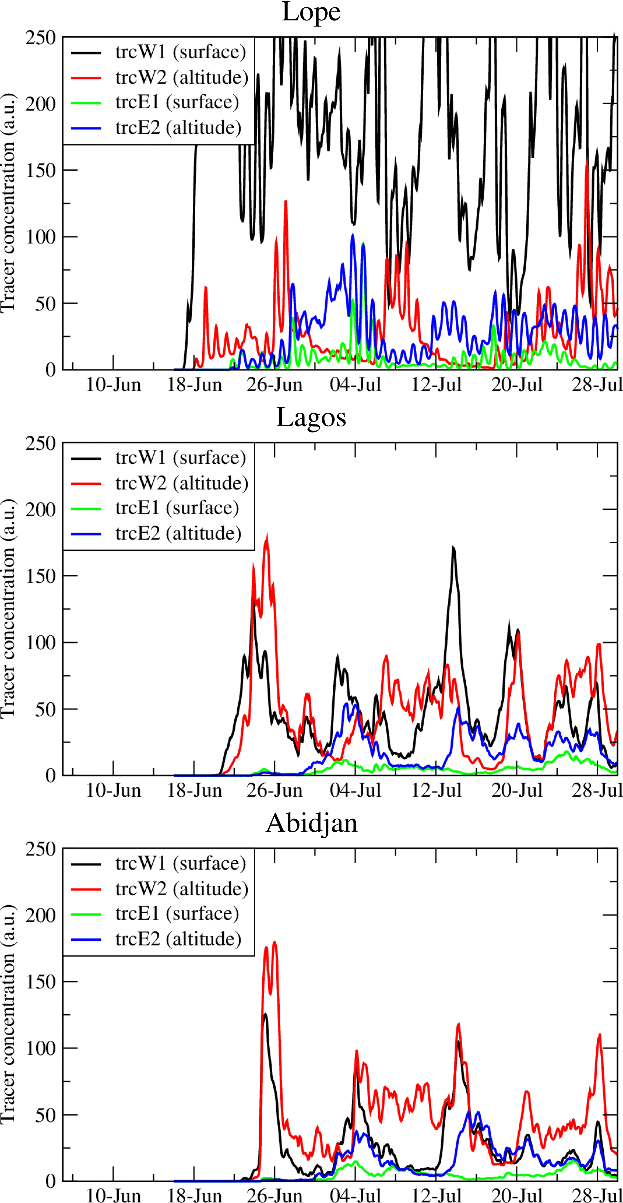
Figure 3Time series of surface concentrations (arbitrary units) in Lope, Lagos, and Abidjan for the four tracer releases from 15 June to 31 July 2014 and close to the most important biomass burning emission areas observed in Central Africa.

Figure 4Regional distribution of tracer surface concentrations (arbitrary units) on 27 July 2014 at 12:00 UTC for each of the tracer experiments, namely trcW1, trcW2, trcE1, and trcE2.
Lope is close to the most important biomass burning observed during the modelled period. The tracers are first emitted on 15 June and the first non-zero tracer concentrations in Lope are modelled on 17 June. As expected, the most important tracer concentrations are modelled for the trcW1 experiment (i.e. trcW experiment with the PR1 injection profile), the site being very close to the source. The values are important (up to 500 in arbitrary units). For the same release source but emitted at altitude, the tracer concentrations from the trcW2 experiment are lower but not negligible. This shows that even if a tracer is emitted between 3000 and 6000 m a.g.l., the daily dry convection in the lower troposphere is strong enough to mix significant concentrations down to the surface layer. The tracer experiments further east (i.e. trcE1 and trcE2) also have non-negligible concentrations in the surface layer in Lope. The first non-zero tracer concentration values are modelled on 23 June, 8 days after the initial tracer emissions. This means that even though the emissions are far to the east, the mixing and long-range transport brings biomass burning aerosols to the west coast of Central Africa in 1 week.
Even if Lagos and Abidjan are far from the tracer sources (≈ 1000 km), the biomass burning proxies also exhibit significant concentrations at the surface in the area of those cities. The most important concentrations are modelled for the tracer emissions in the western domain. For this location, the peak values are not completely correlated in time and depend on the altitude of injection. This shows that the main biomass burning plume follows the same transport in the troposphere, but also that vertical mixing coupled with differential advection may change the transport pathways to the surface layer of the studied cities. Finally, note that in Abidjan, the highest impact is related to the injection of particles at altitude (i.e. in the trcW2 experiment) and not to injection in the ABL (i.e. in the trcW1 experiment). The tracer concentrations in Abidjan and Lagos for the trcE1 and trcE2 experiments are 4 to 5 times lower than for the trcW1 and trcW2 experiments, indicating that most of the tracers are transported away from the Gulf of Guinea northern coast.
3.4 Regional distribution of tracer concentration at the surface
To increase our understanding of the complex transport pathways of biomass burning aerosols, we analyse the regional distribution of tracer concentration at the end of the period covered by the tracer simulations, during which long-range transport pathways from Central Africa to the Gulf of Guinea cities are best established.
Figure 4 presents surface concentrations for 27 July 2014 at 12:00 UTC and for each of the four tracer experiments. This day was selected as an example because it corresponds to (i) the end of the modelled period when the biomass burning transport is the highest, and (ii) the availability of CALIOP data with biomass burning plumes. As previously discussed, the tracers in all experiments reach the Gulf of Guinea cities of Lagos and Abidjan. The most important transport from the fire region to these cities is associated with the western tracer experiment trcW. For trcW1, the main transport from the emission region is to the south and the north-east. Up to latitude ∘ N, the direction of the tracer transport changes and follows the Harmattan (a dry and dusty north-easterly wind) towards the west. The most important contribution comes from the tracer emitted at altitude, i.e. in trcW2. A large part is observed in the southern part of the emission region, while another contribution follows the coastline towards the north and Nigeria before veering to the west upon reaching West Africa and being advected over Lagos and Abidjan.
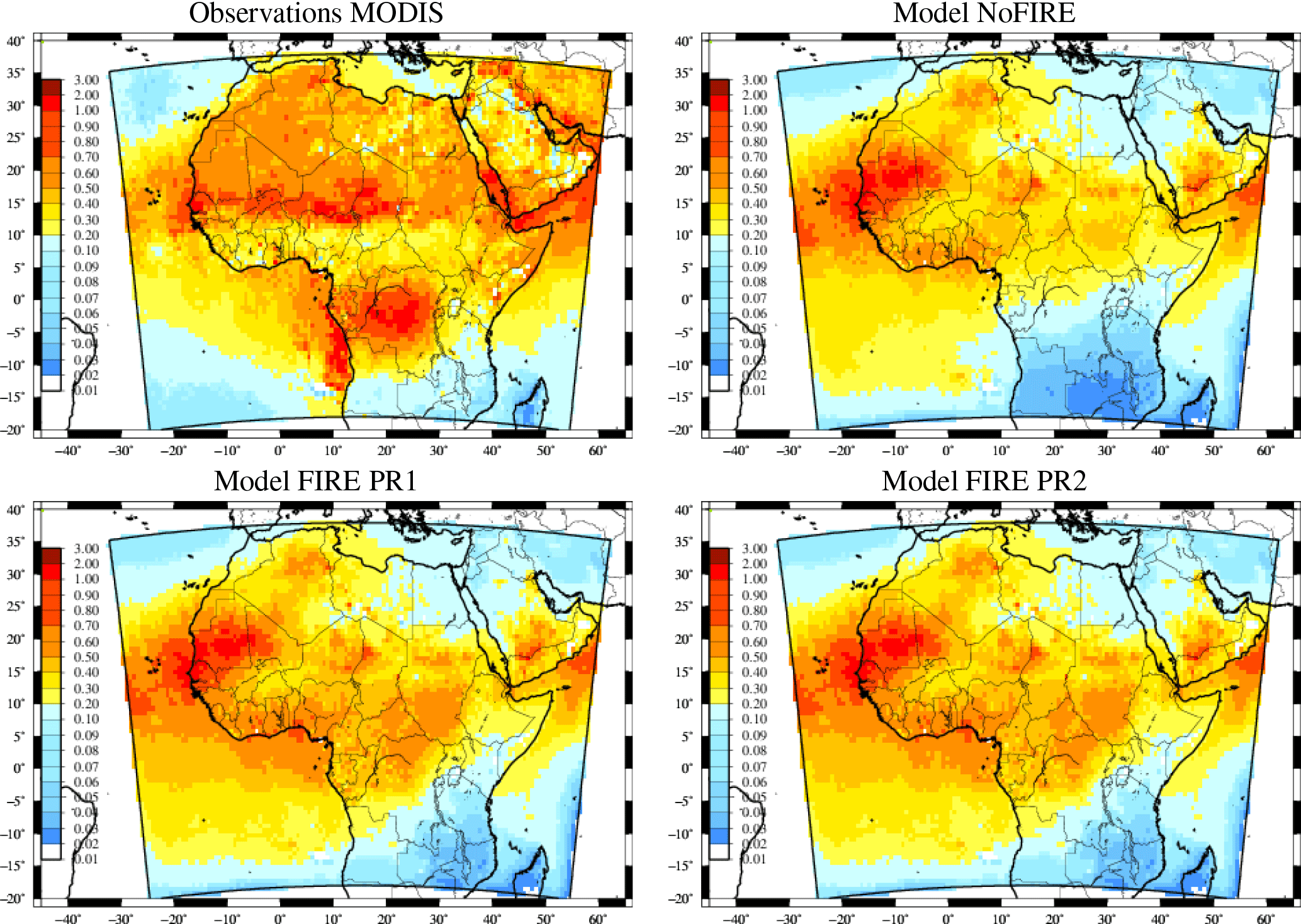
Figure 5Monthly averaged horizontal distribution of AOD (550 nm) for MODIS and CHIMERE simulations NoFIRE, FIRE PR1, and PR2.
For trcW2, the main part of the tracer plume is transported to the east over the continent. Upon reaching longitudes higher than λ>20∘ N, a part of this plume is redirected towards the west as a result of interactions with the Harmattan. Even though less important than for trcW1, a non-negligible part of trcW2 tracers is observed in Lagos and Abidjan.
This tracer experiment allows us to better understand the complex transport pathways of the biomass burning aerosols from Central Africa to the cities of Lagos and Abidjan. This can be summarized as follows.
-
Over continental Central Africa, the main transport pathway for biomass burning aerosols is towards the north-east. For fires, in the western part of the emissions region, the aerosol plume may follow the coastline.
-
The biomass burning products, mainly occurring during the day, are rapidly mixed in the boundary layer. This boundary layer is very deep and may reach 3000 to 4000 m a.g.l. This means that a few hours after the emissions, a vertically constant profile is being advected.
-
The part of the plume going to the west is already vertically well mixed when it passes from land to sea. A part is thus transported in the marine layer and another part above the marine layer in a well stratified layer in the free troposphere.
-
Whatever the emissions location and the injection height, the plume systematically changes direction upon arriving at latitude ∘ N; it is then transported to the south-west, following the Harmattan flow.
The main conclusion regarding the tracer experiments is that the whole area of biomass burning in Central Africa is impacting the surface concentrations in the Gulf of Guinea coastal cities. The second main conclusion is that wildfire particle injection profiles PR1 and PR2 (peaking in the lower and the mid-troposphere, respectively) lead to different biomass burning transport pathways. Nevertheless, after a few weeks, the fire emissions injected in the mid-troposphere have an impact on the Gulf of Guinea cities of the same order of magnitude as those emitted in the boundary layer.
Before analysing local pollution, it is necessary to have a synoptic view of the long-range transport of pollutants. In the previous section, it was shown that the meteorological conditions are favourable for importing Central African pollutants to the Gulf of Guinea coast. In this section, using available observations and simulations with realistic emissions, transport and chemistry are used in order to quantify the model ability to retrieve the variability and intensity of the main pollutants.
4.1 AOD CHIMERE vs. MODIS
Results are presented in Fig. 5 for the month of July 2014, when biomass burning intensity is at its maximum for the studied period. The satellite observations are compared to the three model configurations NoFIRE, FIRE PR1, and FIRE PR2.
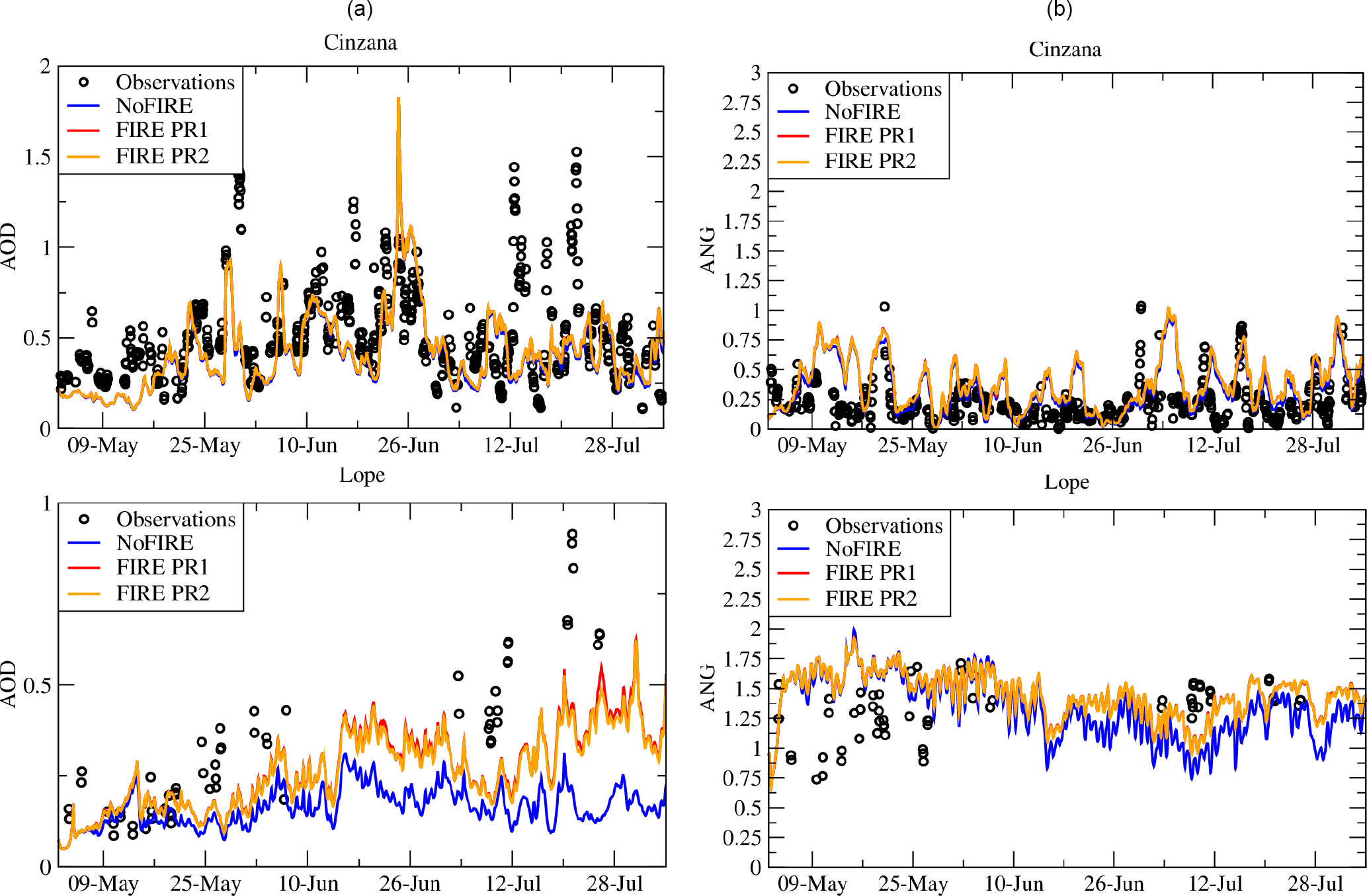
Figure 6Comparison of AERONET measurements and model results for AOD (a) and the Ångström exponent (b). Time series are presented for the Cinzana and Lope stations and for the whole modelled period.
Over Africa, the MODIS data show two large areas of AOD > 0.5: in Central Africa (corresponding to fire emissions) and up to latitude 10∘ N (corresponding to mineral dust emissions). Without fire emissions, the NoFIRE simulation enables the validation of the mineral dust modelling and shows that the model tends to underestimate the AOD over the Sahel between 10 and 15∘ N. On the other hand, the plume transported to the Atlantic is slightly overestimated. Over the Gulf of Guinea, the modelled AOD is overestimated (0.5 when MODIS shows 0.3). The AOD due to mineral dust is mostly underestimated and many factors may explain this. As already discussed in Menut et al. (2016), the modelled size distribution may be inaccurate, while it is very sensitive for the AOD estimation. It was also shown that a bias in AOD calculation may exist but is not necessarily related to erroneous modelled surface concentrations of particulate matter (PM). Over this region and during this period, an additional explanation for this bias could be related to the way the model handles precipitation events. The results presented in Appendix C, dedicated to the analysis of the precipitation, show that the modelled precipitation patterns correspond to what was observed with the Met Office MIDAS land surface stations. However, as discussed in Ruti et al. (2011), Flaounas et al. (2011), and Efstathiou et al. (2013), these processes remain highly variable, uncertain, and difficult to validate, and it is possible that the scavenging was not modelled correctly, leading to these differences between the model and observations.
When including the calculation of biomass burning emissions and their transport, a general increase is observed in the FIRE simulations. While AODs are less than 0.05 in the NoFIRE simulation, AOD values can reach 1 over Cameroon in the FIRE simulations. The westerly winds transport these biomass burning plumes over the Gulf of Guinea and the model results shows that the whole coast is under these dense plumes, from Nigeria to the Ivory Coast. With MODIS, two high AOD regions related to fires are observed: one in Central Africa and the other along the coast. With the model, the increase in AOD is located more to the north and less intense. Finally, it is worth noting that there are no significant differences between the results of the two FIRE (using PR1 and PR2) simulations.
The conclusion is that the model reproduces the two large areas of high AOD due to mineral dust and biomass burning emissions, but that the intensities are not correctly modelled. Over Central Africa, the modelled AODs due to biomass burning are underestimated. This may be due to fire intensity or the size distribution of the modelled aerosol. This will be further discussed in Sect. 4.3 with the comparison between observed and modelled CO.
4.2 AOD and Ångström coefficient CHIMERE vs. AERONET
Table 2Correlations between observations (AERONET) and the model (CHIMERE PR2) for aerosol optical depth (AOD). F is 0 for the NoFIRE simulation and 1 for the simulation with fire emissions. N is the percentage of hourly available measurements, Rt is the temporal correlation, and the bias is calculated by using the difference (model minus observation).
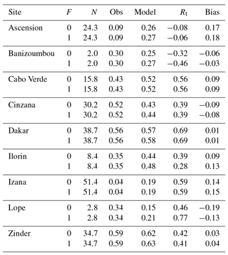
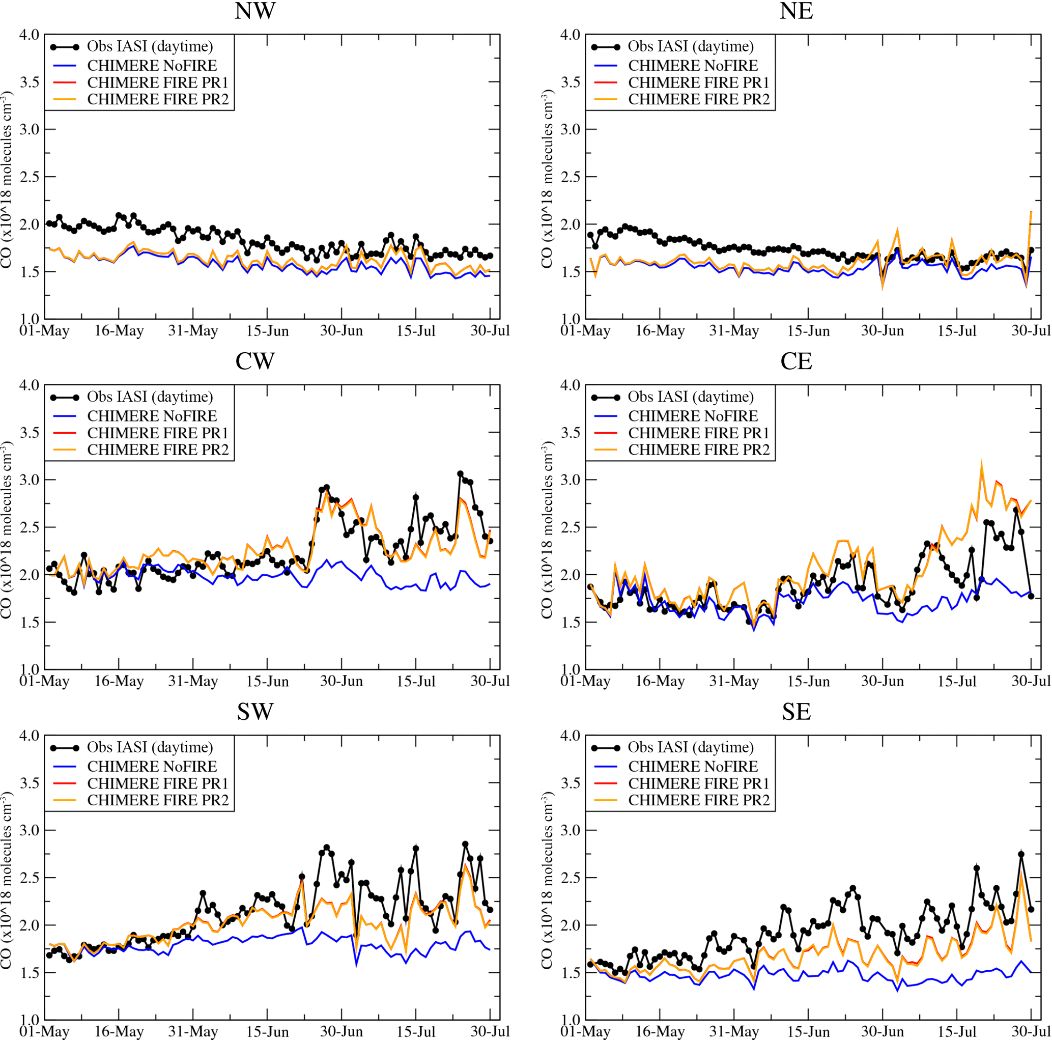
Figure 7Time series of vertically integrated carbon monoxide (CO column) in 1018 molecules cm−2 for IASI and for the simulations with CHIMERE.
Results are presented as statistical scores in Table 2. For the time series, the two FIRE simulations using PR1 and PR2 are displayed. But for the scores, only the results for FIRE PR2 are presented, with the differences between the two FIRE simulations being negligible.
Except for the station of Lope, differences between the simulations NoFIRE and FIRE are very small (Table 2). The correlation values range between −0.08 (Ascension) and 0.77 (Lope). The low score in Ascension is related to the offshore location of the site and the fact that long-range transport over the sea is difficult to reproduce: being less turbulent, there is less horizontal diffusion and vertical mixing. The plumes are thinner and more concentrated, and the results are more sensitive to a possible model error in the wind direction. The comparison with observations located at one single point over the sea thus often exhibits a lower correlation than for comparisons conducted over land. For other sites, the correlations are larger and show that the mineral dust variability is well modelled. The only site with differences between the NoFIRE and FIRE simulations is Lope, close to the biomass burning areas. The correlation increases from 0.46 to 0.77 when biomass burning emissions are added. This shows that the timing of the fire emissions and the transport is precise enough to clearly improve the simulation.
Examples of detailed comparisons between AERONET and the model are displayed in Fig. 6. In Cinzana, the AOD hourly variability is well represented and the majority of observed AOD peaks are modelled. The site being mainly under the influence of mineral dust emissions, there is no significant difference between NoFIRE and FIRE. This is very different in Lope. The addition of the biomass burning emissions increases AOD during the whole period. The modelled AOD remains lower than the observations, but the timing and the absolute value are more realistic.
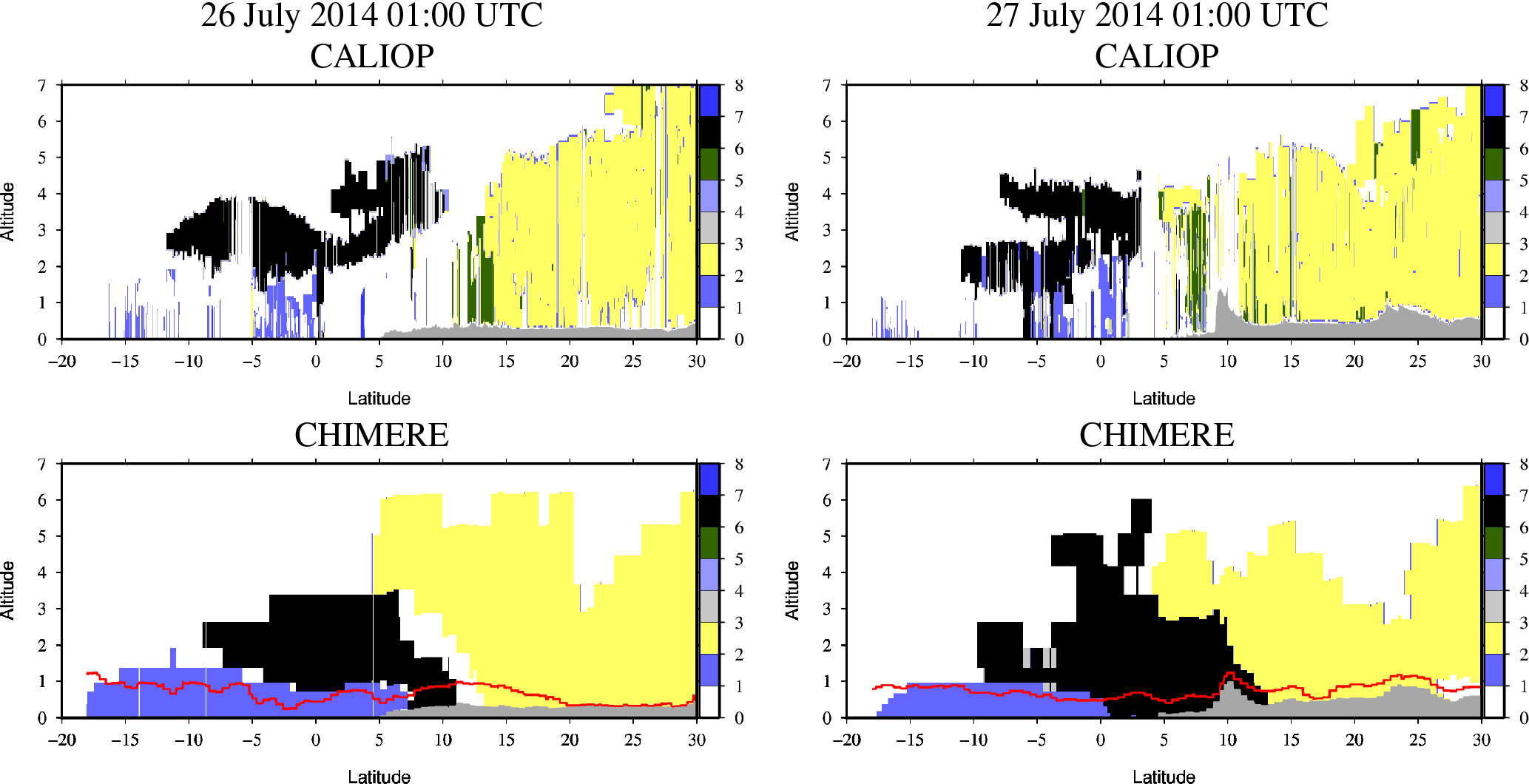
Figure 8Vertical cross section of CALIOP aerosol types and comparison to the CHIMERE FIRE simulation. The colour bar is related to the CALIOP classification: (0 : 1) not applicable, (1 : 2) clean marine, (2 : 3) dust, (3 : 4) polluted continental or smoke, (4 : 5) clean continental, (5 : 6) polluted dust, (6 : 7) elevated smoke, and (7 : 8) dusty marine. For the model, the boundary layer height is superimposed in red.
As opposed to the comparison with MODIS, these time series and correlation values show that the AOD is not always overestimated by the model. This result shows the large variability obtained with different sets of data and also reflects the difficulty of modelling this parameter, which is strongly dependent on the optical properties of the modelled aerosols and the estimation of the extinction with the modelled size distribution (in our configuration, 10 bins may be considered as a correctly resolved size distribution for a CTM).
Complementary to the AOD, the Ångström exponent is also compared to the AERONET retrievals and for the same two stations of Cinzana and Lope. Results are presented in Fig. 6 (right column). This exponent expresses the ratio between the AODs at two different wavelengths and its value is inversely proportional to the aerosol size. Low values of the Ångström exponent will be representative of mineral dust (aerosols mainly in the coarse mode), while high values will be representative of biomass burning. In Cinzana, the Ångström exponent is low, with values between 0 and 0.3 (except some peaks). This means that the aerosol content is mainly mineral dust. On the other hand, in Lope, the Ångström exponent is higher and values range between 1 and 1.75, which is representative of finer particles and thus concentrations related to biomass burning emissions.
4.3 CO CHIMERE vs. IASI
The CO comparison is presented in Fig. 7 as time series with the daytime IASI measurements and the corresponding model results. Each time series corresponds to the sub-domains described in Fig. 1.
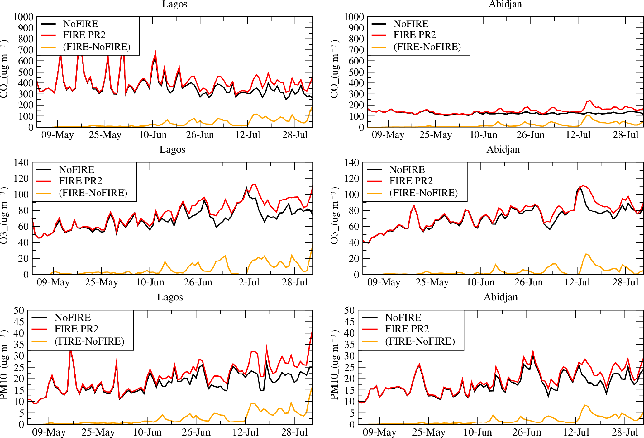
Figure 9Time series of surface concentrations (in µg m−3) of CO, O3, and PM10. Results are presented for Lagos and Abidjan and for the simulations NoFIRE and FIRE PR2.
The IASI data show the increase in vertically integrated CO concentrations over Central Africa and the eastern Atlantic from May to July (sub-domains SW and SE): under the influence of biomass burning emissions, the CO concentrations increase by 100 %, from ≈ 1.5 × 10¹⁸ to ≈ 3 × 10¹⁸ molecules cm−3.
For NoFIRE, the CO concentrations are quasi-constant. For FIRE, the observed CO increase is correctly reproduced. Even though this increase is slightly underestimated by the model in the southern part (SW and SE), the temporal variability and intensity are better modelled in the central part (CW and CE) where the studied cities are located. North of the studied region (NW and NE), the biomass burning emissions have a very low impact on the CO concentrations, with the outputs of NoFIRE and FIRE being close. At this latitude, the model tends to slightly underestimate CO concentrations (by ≈ 0.2 × 10¹⁸ molecules cm−3) with respect to IASI.
The differences between observations and the model may be due to several factors. First, the boundary conditions used for the simulations are global and “climatological” in model outputs. The transition from “mean” time-averaged values and this real test case may induce biases due to the lack of temporal variability in the climatologies. For long-lived species such as CO, these biases may be transported inside the model domain. Secondly, underestimated CO may be due to overestimated OH or to an underestimate of the production of CO from the oxidation of VOCs. Zeng et al. (2015) showed that this last process results in a large variability in model results. However, without complementary observations it remains difficult to disentangle different contributions.
4.4 CHIMERE vs. CALIOP aerosol sub-types
The vertical cross sections of aerosol types derived from CALIOP observations and CHIMERE simulations along the CALIPSO track for 26 and 27 July 2014 are displayed in Fig. 8. We focus on these two days because (i) CALIOP data are available above the studied region, and (ii) the long-range transport of biomass burning is at a maximum at the end of the studied period. The two CALIOP ground tracks are shown in Fig. 1.
The first result with this comparison is that the aerosol characteristics of the main air masses are well reproduced by the model: over land, the main aerosol is mineral dust, while over sea, sea-salt aerosols dominate the composition near the surface. Over sea at altitude, the main aerosol type is related to biomass burning (denoted as smoke). For the two days, the model is able to estimate the latitudinal extension of the smoke plume, from −15 to +10∘ N. Regarding the vertical extension of smoke, the model underestimates the altitude of the top of the plume on 26 July but represents it correctly for 27 July. For this latter day, the vertical structure of the plume (exhibiting two distinct features) is correctly reproduced by the model. The main difference between the model and the observations is that the smoke plume reaches the surface with the model but not in the observations. Jethva et al. (2014) pointed out that in the case of an optically thick aerosol layer, the sensitivity of the CALIOP backscattered signal to the altitude of the base of the aerosol layer is strongly attenuated by the two-way transmission term. As a result, the operational algorithm may locate the base of the aerosol layer too high when it could actually be deeper and extend towards the surface.
However, the CALIOP data are only for “elevated smoke” (see Appendix B), meaning that this is not because the CALIOP aerosol typing algorithm did not detect and attribute a smoke value above the marine layer but rather that there is no smoke. In this sense, the model provides complementary insight about the plume vertical extent.
Finally, this comparison with “instantaneous” measurements in the whole troposphere proves that the model is able to correctly estimate the location, latitude, and altitude of the main studied aerosols. This improves our confidence in the model robustness.
In this section, we focus on the atmospheric composition in coastal urbanized areas. The analysis is carried out with the model only, as no data are available in the region and for the studied period. Results are presented for the sites Lagos (Nigeria) and Abidjan (Ivory Coast), which are representative of strongly urbanized coastal areas in the Gulf of Guinea. The surface concentrations of three chemical species are presented: (i) O3, a secondary species produced by anthropogenic, biogenic, and fire emissions, (ii) CO, a gaseous species primarily emitted by anthropogenic and fire emissions, and PM10, which is representative of the sum of aerosol produced by anthropogenic and natural sources.
Time series of surface concentrations of CO, O3, and PM10 are presented in Fig. 9. The figure shows the concentrations for NoFIRE and FIRE, as well as the difference (FIRE–NoFIRE). For the three species and in both cities, the impact of biomass burning appears after a few days. This impact has the same order of magnitude for the two sites, highlighting the widespread nature of long-range transport form Central Africa. The maximum contribution of the biomass burning emissions is ≈ 150 µg m−3 for CO, ≈ 20 µg m−3 for O3, and ≈ 5 µg m−3 for PM10. The contribution of fires appears as a smooth but steady increase and does not generate pollution peaks, which is consistent with continuous wildfire emissions and uninterrupted long-range transport towards the Gulf of Guinea.
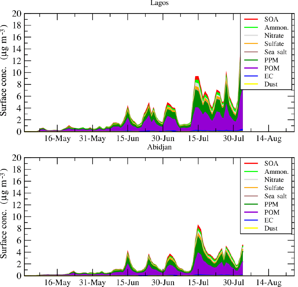
Figure 10Time series of daily averaged surface concentrations of differences PM10(FIRE)–PM10(NoFIRE) (in µg m−3). The speciation is presented for all aerosol species modelled with CHIMERE.
The PM10 is the cumulated mass of several aerosol types. With the model, it is possible to quantify the contribution of each type of aerosol (Menut et al., 2016). Results are presented for Lagos and Abidjan in Fig. 10 as differences between the simulations FIRE and NoFIRE in order to quantify the speciation of the additional amount of aerosols due to biomass burning.
The composition of the aerosol related to fires is mainly composed of primary organic matter (POM) and primary particulate matter (PPM). To a lesser extent, the aerosol is also composed of ammonium, sulfate, and secondary organic aerosol (SOA).
This study examined the atmospheric composition during the summer of 2014 (from May to July) in the region of the Gulf of Guinea. The main goal was to quantify the relative contribution of biomass burning emissions occurring in Central Africa for aerosol (i.e. PM10), CO, and O3 surface concentrations in large urbanized areas such as Lagos and Abidjan. It was conducted in the framework of the DACCIWA European project, aiming to observe and model the interactions between dynamics, clouds, and aerosols in the Gulf of Guinea.
The period was modelled with the meteorological model WRF and the chemistry-transport model CHIMERE. Several model configurations were used. First, in order to know if the biomass burning pollutants reach the Gulf of Guinea cities (e.g. Lagos and Abidjan), a tracer experiment was performed. It was shown that, independently of the location of emissions in Central Africa, biomass burning always impacts the surface concentrations of pollutants in those cities. Depending on the location of the emissions, the fire plumes may follow the west coast of Central Africa to reach the cities (the most direct transport pathway) or may be advected towards the east over continental Africa and reoriented toward the cities by the north-easterly Harmattan winds. In order to gain insight into the impact of biomass burning emissions injection in the atmosphere, two simulations were performed with different vertical injection profiles, one peaking in the lower troposphere and one peaking in the mid-troposphere. It was shown that resulting tracer surface concentrations were not sensitive to the shape of the profile. The reason is that, during a fire, the pyroconvection induces a strong and fast mixing of the surface flux. Whatever the shape of the injection profile, the pollutants are quickly mixed in the vertical before being transported over long distances.
The simulations with realistic biomass burning emissions were analysed by comparison to numerous datasets: CO from IASI, AOD from MODIS and AERONET, surface concentrations of PM10 from the Sahelian Dust Transect data, and aerosol sub-type classification from CALIOP. It was shown that the model is able to reproduce the physical and chemical characteristics of the emitted gas and aerosol species due to biomass burning. In addition, and using the vertical information provided by CALIOP, it was shown that the location and altitude of the several aerosol plumes (mineral dust and biomass burning) are correctly modelled.
Finally, and by a comparison of simulations without fire emissions (NoFIRE) and simulations with fire emissions (FIRE), a first quantification of the amount of additional pollutants in Lagos and Abidjan was presented. It was shown that biomass burning will induce a regular increase in surface concentrations of pollutants during the whole studied period with the order of magnitude of ≈ 150 µg m−3 for CO, ≈ 20 µg m−3 for O3, and ≈ 5 µg m−3 for PM10. Using the modelled speciation, this additional amount was shown to be mainly composed of POM and PPM.
This study shows that an understanding of atmospheric pollution for urbanized areas in the Gulf of Guinea region must take into account biomass burning in Central Africa. The numerous chemical species contained in the fires plumes are involved in the budget of air quality and their concentrations will directly affect human health (Knippertz et al., 2015). In this study, the model configuration was off-line and this may induce a bias in the result: the direct effect of dense biomass burning plumes may directly affect the convection in the region and the large amount of aerosols may also change the precipitation via indirect aerosol effect. The next step will be to study this interaction using an online coupled modelling system.
All simulations presented in this article are available on request to the first author.
A1 The WRF meteorological model
The meteorological variables are modelled with the non-hydrostatic WRF regional model in its version 3.6.1 (Skamarock et al., 2007). The global meteorological analyses from the National Centers for Environmental Prediction (NCEP) with the Global Forecast System (GFS) products are used to nudge WRF hourly for pressure, temperature, humidity, and wind. In order to preserve both large-scale circulations and small-scale gradients and variability, the “spectral nudging” technique was applied. This nudging was evaluated in regional models, as presented in Von Storch et al. (2000). In this study, the spectral nudging was selected to be applied for all wavelengths greater than ≈ 2000 km (wave numbers less than 3 in latitude and longitude for wind, temperature, and humidity and only above 850 hPa). This configuration allows the regional model to create its own dynamics, thermodynamics, and composition features within the boundary layer and ensures that the large scale follows the thermodynamic fields from the analyses.
The model is used with 28 vertical levels from the surface to 50 hPa. The Single Moment 5-class microphysics scheme is used, allowing for mixed phase processes and supercooled water (Hong et al., 2004). The radiation scheme is the RRTMG scheme with the MCICA method of random cloud overlap (Mlawer et al., 1997). The surface layer scheme is based on Monin–Obukhov with a Carlson–Boland viscous sub-layer. The surface physics is calculated using the Noah Land Surface Model scheme with four soil temperature and moisture layers (Chen and Dudhia, 2001). The planetary boundary layer physics is processed using the Yonsei University scheme (Hong et al., 2006), and the cumulus parameterization uses the ensemble scheme of Grell and Dévényi (2002). The aerosol direct effect is taken into account using the Tegen et al. (1997) climatology.
A2 The CHIMERE chemistry-transport model
CHIMERE is a chemistry-transport model allowing for the simulation of concentration fields of gaseous and aerosol species on a regional scale. It is an off-line model driven by precalculated meteorological fields. In this study, the version fully described in Menut et al. (2013a) and updated in Mailler et al. (2017) is used. If the simulation is performed with the same horizontal domain, the 28 vertical levels of the WRF simulations are projected onto 20 levels from the surface up to 200 hPa for CHIMERE. The CHIMERE vertical levels increase in depth from the surface to the top. The altitudes (above ground level) of the first four vertical layers are ≈ 18, 42, 75, and 115 m, respectively. Being expressed in σ pressure coordinates, the layer depths are not constant in space and time and are able to follow the surface pressure evolution and the topography.
The chemical evolution of gaseous species is calculated using the MELCHIOR2 scheme. The photolysis rates are explicitly calculated using the FastJX radiation module (version 7.0b) (Bian and Prather, 2002; Wild et al., 2000). The aerosols are modelled using the scheme developed by Bessagnet et al. (2004). The aerosol size is represented using 10 bins from 40 nm to 40 µm in mean mass median diameter (MMMD). The aerosol life cycle is completely represented with the nucleation of sulfuric acid, coagulation, absorption, wet and dry deposition, and scavenging. The scavenging is represented by in-cloud and sub-cloud scavenging.
The aerosol model species and their characteristics consist of 10 different types of aerosols, some being a compound of several aerosol species. In the Results section, these species are represented as follows: PPM is for anthropogenic primary particulate matter, DUST is for mineral dust, EC is for elemental carbon, POM is for primary organic matter, SALT is for sea salts, and SOA is for secondary organic aerosols. SO4, NO3, and NH4 are equivalents of sulfate, nitrate, and ammonium, respectively. WATER is for water. More details are provided in Menut et al. (2013a, 2016).
The modelled AOD is calculated by FastJX for several wavelengths over the whole atmospheric column, as detailed in Menut et al. (2016). At the boundaries of the domain, climatologies from global model simulations are used. In this study, outputs from LMDz-INCA (Hauglustaine et al., 2014) are used for all gaseous and aerosols species, except for mineral dust for which the simulations from the GOCART model are used (Ginoux et al., 2001).
The anthropogenic emissions are issued from the Hemispheric Transport of Air Pollution (HTAP) global database (Janssens-Maenhout et al., 2015). These emissions are provided as gridded maps for each month of the year. For the simulation, weekly profiles are applied to include weekdays, Saturdays, and Sundays. In addition, hourly profiles are applied to have an hourly variability also depending on the activity sector. The complete calculation of these fluxes is detailed in Menut et al. (2012) and Mailler et al. (2017).
The mineral dust emissions are calculated using the Alfaro and Gomes (2001) scheme, optimized following Menut et al. (2005), and use the soil and surface databases presented in Menut et al. (2013b). Since this latter article, several changes have been made in the emissions scheme. They are all related to the spatial extent of the emissions flux calculations: from the Sahara only to any arid or semi-arid areas in the world. The surface and soil databases being global, the fluxes are now systematically calculated over the whole domain, including non-desert areas such as Europe. In order to keep realistic fluxes under a variety of meteorological conditions, the emissions scheme was adapted. These changes are active for all model cells including the desert ones. These changes are briefly described below.
The erodibility is diagnosed using the United States Geological Survey (USGS) land use and an additional database, which was built using MODIS surface reflectance (Beegum et al., 2016). For all model cells considered as “desert”, the MODIS erodibility is used, while for all other cells, a constant erodibility factor is applied depending on the USGS land use, as in Menut et al. (2013b). To take into account the rain effect on mineral dust emissions limitation, a “memory” function is added. During a precipitation event, the surface emissions fluxes are set to zero. After the precipitation event, a smooth function is applied to account for a possible crust at the surface and thus fewer emissions (Mailler et al., 2017).
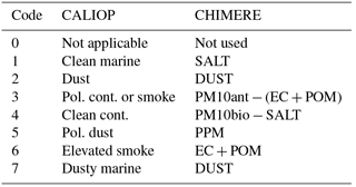
The equivalent of the CALIOP aerosol classification is obtained from CHIMERE using aerosol concentrations directly. The depolarization not being modelled, we have to find other ways to reproduce the CALIOP classification. The following assumptions are made.
-
The CALIOP terminology “elevated smoke” is difficult to evaluate in terms of altitude. In Omar et al. (2010), it is stated that thin aerosol layers are “clean continental” close to the surface or “smoke” if they are elevated. Over the ocean, all elevated non-dust aerosol layers are identified as smoke.
-
CALIOP is particularly sensitive to clouds and Chen et al. (2012) noted that CALIOP often misidentifies aerosol as clouds. In Winker et al. (2013), “elevated layers” are considered as those up to 2 km above ground level.
-
In this study, we make no difference between “dust” and “dusty marine”: this is mineral dust.
-
Many CALIOP profiles contain “not applicable” values. This means that the detection algorithm was not able to affect an aerosol type. This is not the case with the model, in which for each profile and each altitude, we are able to diagnose the major aerosol contribution, thereby increasing the information content with respect to CALIOP products.
The other hypotheses made to match as best as possible the CALIOP “optical indexes” with CHIMERE “aerosol concentrations” are described in Table B1. The model species are, in general, directly linked to the CALIOP classification. As the model is able to separate PM from anthropogenic and biogenic origin (Menut et al., 2013a), we use it to distinguish the “polluted continental” and “clean continental” aerosol layers. For the biomass burning emissions products, the “smoke” is considered as the sum of elemental carbon (EC) and POM.
Table B1Correspondence between CALIOP “optical indexes” and CHIMERE “aerosol concentrations”.
The studied period corresponds to a specific and complex meteorology. In this section, we focus on precipitation near the coastline where various precipitating systems occurred during the period from May to August; Fig. C1. This constrains the transport of local emissions and impacts the wet deposition of emitted species.
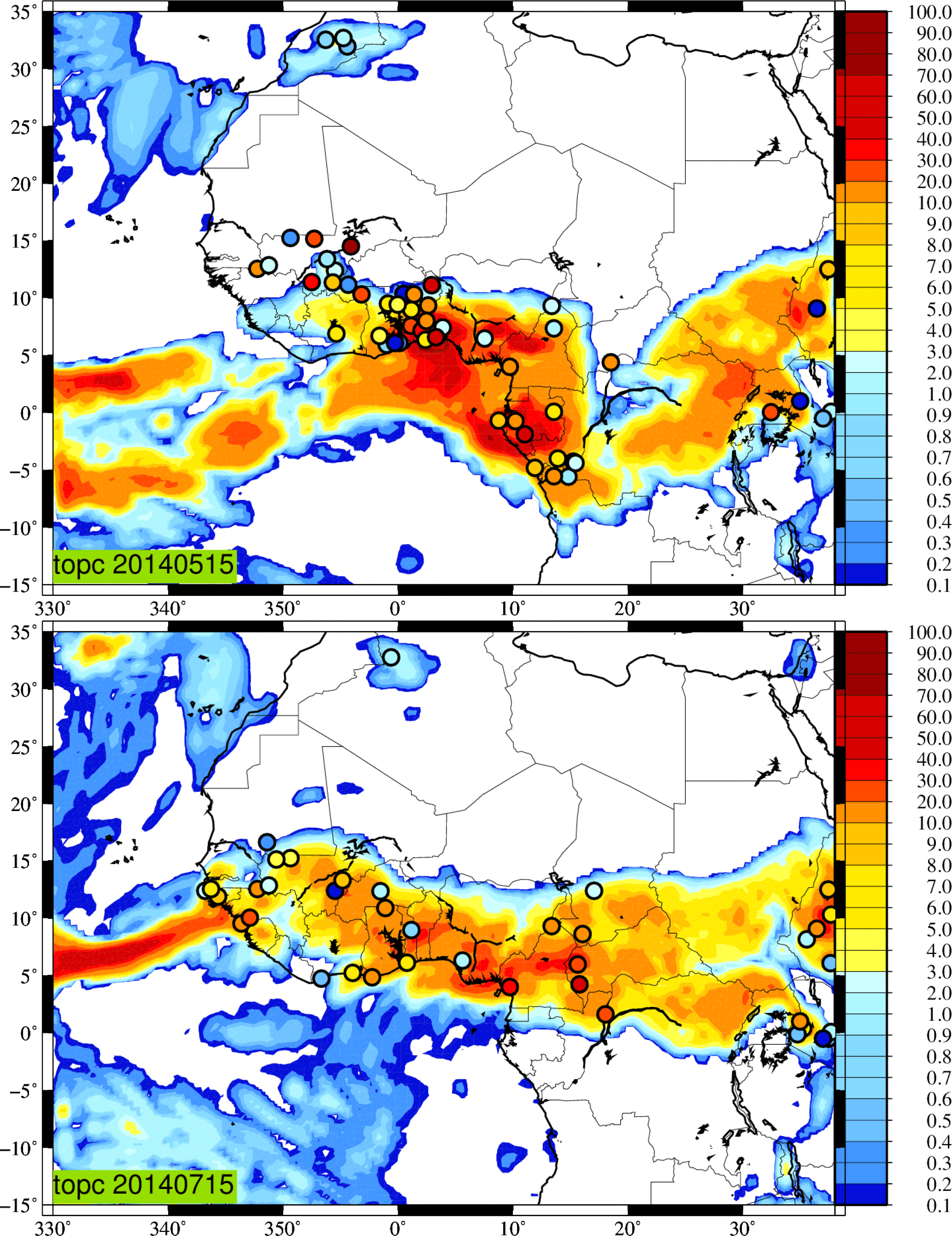
Figure C1Comparison between observed and modelled daily cumulated precipitation rate (mm day−1) for 15 May and 15 July 2014. For the precipitation measurements, only the non-zero daily cumulated values are reported on the plot.
Time series of comparisons are presented in Fig. C2 for the highly urbanized coastal cities of Lagos and Abidjan. The observations are from the Met Office MIDAS land surface stations data (http://data.ceda.ac.uk/badc/ukmo-midas/). They are provided with a 3-hourly time step and are daily accumulated. In Lagos, the observed precipitation rate is sporadic but intense, with values up to 60 mm day−1 five times during the period. For May and June, the model simulates lower values for these events. During July, the model simulates the two largest precipitation events on 2 and 18 July, but with a time shift of 1 to 2 days, respectively. Furthermore, the model produces rain every day, unlike what is observed, thereby overestimating the number of rainy days. This will likely lead to an underestimation of the modelled surface concentrations due to the enhanced simulated wet scavenging in the lower troposphere. In Abidjan, the observed precipitation rate is more important and frequent. The simulation is more realistic and there is a better agreement between the number of rainy days and the 24 h accumulated precipitation. The two rainiest periods, around 15 June and 1 July, are well simulated, with rainfall amounts in excess of 50 mm day−1.
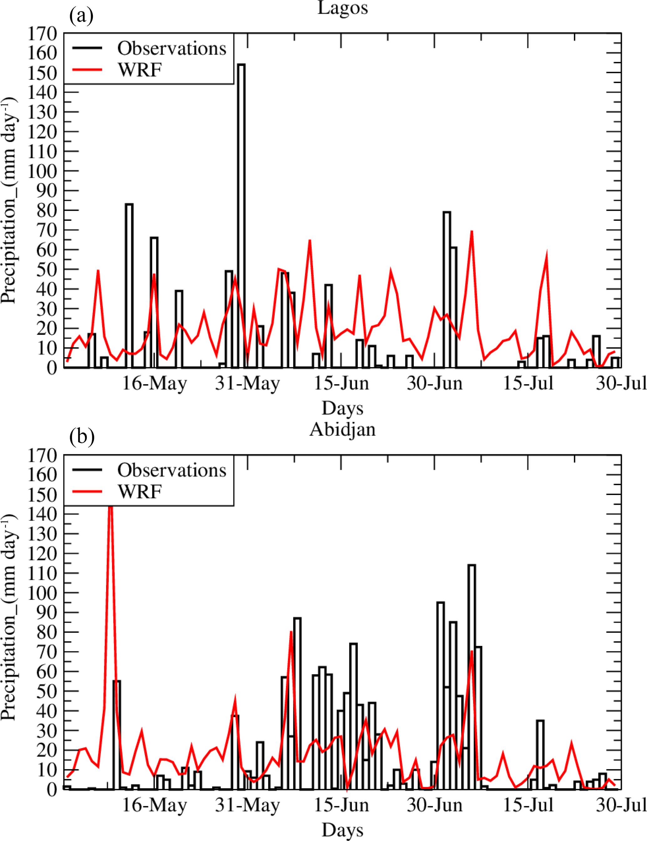
Figure C2Time series of 24 h accumulated precipitation from the BADC stations and the corresponding model cell: Lagos (a) and Abidjan (b).
The biomass burning emissions fluxes are a forcing delicate to model. Several steps are needed to estimate these fluxes, from the flux at the surface itself, to the way to inject it in the atmosphere. We can split the calculation into three different steps.
-
The emissions fluxes: this is the emitted mass for each chemical species.
-
The injection height: this parameter defines the top altitude of the fire emission vertical plume.
-
The injection vertical profile: having the total emitted mass flux and the top of the plume, it is necessary to define the shape of the vertical injection profile.
The emissions fluxes depend on the burned area, land use, vegetation type, and fuel load. The calculations are performed hourly using the high-spatial-resolution Analysis and Prediction of the Impact of Fires on Air Quality Modeling (APIFLAME) model. All information about this estimation is provided in Turquety et al. (2014). This model was previously used, for example, in Rea et al. (2015). In this APIFLAME model version, fire emissions fluxes are calculated based on the MODIS burned area product MCD64 (Giglio et al., 2010). The emission fluxes being estimated daily, a diurnal profile is applied in which 30 % is redistributed during the night (18:00 to 08:00 LT local time) and 70 % during the day, close to values usually chosen in biomass burning model studies (Zhang et al., 2012). More than 40 chemical species are calculated and then used in the CHIMERE model. An example of the time-cumulated flux of CO for the month of July 2014 is presented in Fig. D1. Emissions related to biomass burning are mainly located in Central Africa.
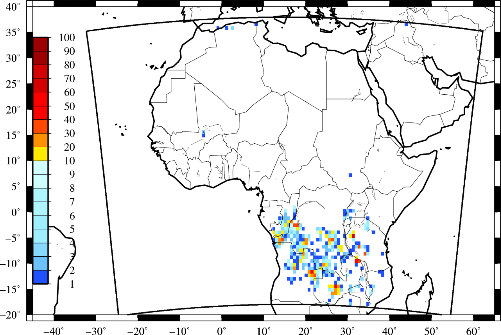
Figure D1Biomass burning emission fluxes of CO (in molecules cm−2 month−1) cumulated over the whole month of July 2014.
For the injection height, Hp, we used the approach proposed by Sofiev et al. (2012). In south-western Africa and during the months of July and August, a typical variability in Hp is estimated between 3 and 4.5 km (Labonne et al., 2007). The calculation of Sofiev et al. (2012) is based on the convective available potential energy estimation, itself diagnosed using the fire radiative power (FRP) of each fire. They validated their Hp calculation using the Multi-angle Imaging SpectroRadiometer plume height retrievals and showed a good agreement between the two. Hp is estimated for each individual fire as
with α=0.24, β=170 m, γ=0.35, δ=0.6, Pf0=106 W, and s−2. The FRP, Pf, is expressed in W (with 1 W = 1 J s m2 kg s−3). NFT is the Brünt–Väisälä frequency in the free troposphere.
An empirical correction is performed for the known underestimation of FRP by MODIS in the case of strong fires (Veira et al., 2015):
with ϵ=0.5 and Hdeep=1500 m.
The last step, the injection vertical profile shape, corresponds to a development specifically carried out for this study.
PM10 CHIMERE vs. surface measurements
The surface PM10 concentrations of the Sahelian Dust Transect (Marticorena et al., 2010) are used to ensure that the aerosol mass is well modelled close to the surface. It is a network of four stations: Banizoumbou (Niger), Cinzana (Mali), M'Bour, and Bambey (Senegal). These stations are collocated with the AERONET stations. The main goal of this network is to have measurements along an iso-latitude transect at ≈ 13∘ N. In the framework of observations and modelling studies, these measurements were already used in Hourdin et al. (2015), for example.
Statistical scores are presented in Table D1 for the PR2 configuration only. Results show that the addition of fire emissions has a very low impact on these surface concentrations. This is mainly due to the fact that the only sites having PM10 surface concentration measurements are located in the northern part of the domain and are not under the effect of biomass burning emissions; they are mostly under mineral dust emissions and transported plumes. This confirms that the fires plumes do not reach this latitude of 13∘ N.
Time series for the site of Cinzana are shown in Fig. D2. Results also show that the PM10 concentrations have a large temporal variability, both in measurements and the model. However, even though the correlations are low, it is shown that the model is able to estimate the amount of mineral dust.
Table D1Correlations between observations (Sahelian Transect) and the model (CHIMERE PR2) for the PM10 surface concentrations. F is 0 for the NoFIRE simulation and 1 for the simulation with fire emissions. N is the percentage of hourly available measurements, Rt is the temporal correlation, and the bias is calculated by using the difference between the observation and the model.
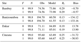
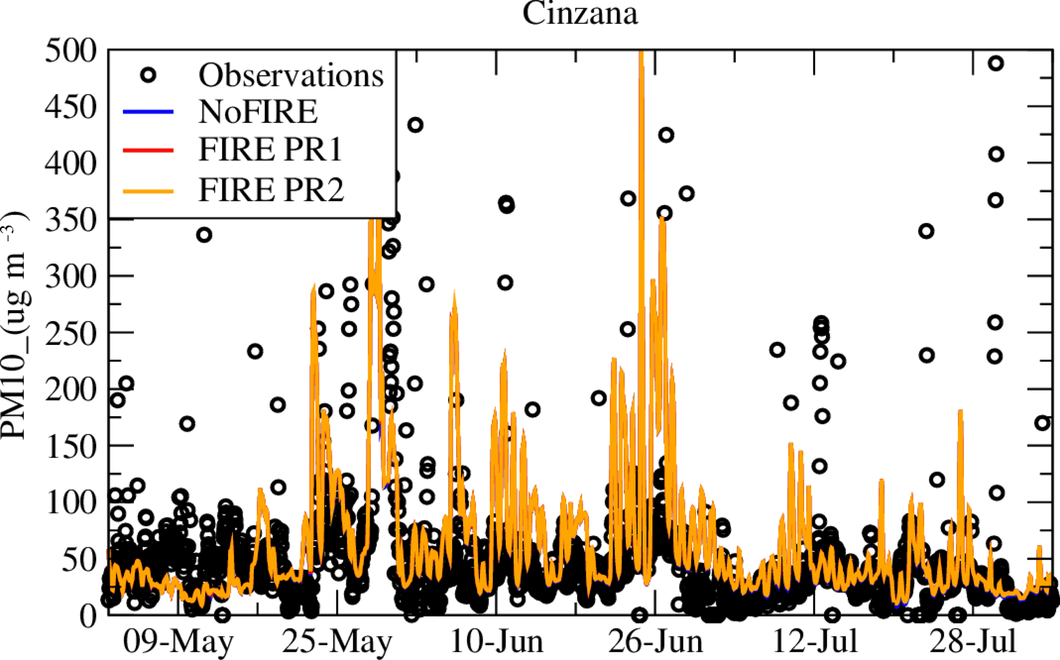
Figure D2PM10 surface concentration time series measured with the Sahelian Transect Network and modelled with the NoFIRE and the FIRE PR1 and PR2 configurations.
The authors declare that they have no conflict of interest.
This article is part of the special issue “Results of the project “Dynamics–aerosol–chemistry–cloud interactions in West Africa” (DACCIWA) (ACP/AMT inter-journal SI)”. It is not associated with a conference.
The research leading to these results received funding from the European
Union 7th Framework Programme (FP7/2007-2013) under grant agreement
no. 603502 (EU project DACCIWA: Dynamics–Aerosol–Chemistry–Cloud interactions
in West Africa). Thanks to the British Atmospheric Data Centre, which is part
of the NERC National Centre for Atmospheric Science (NCAS), for the
meteorological surface data used in this paper. Solène Turquety
acknowledges the French space agency (CNES) for financial support. The IASI
CO data were provided by LATMOS/CNRS and ULB. The MODIS AOD datasets were
acquired from the Level-1 and Atmosphere Archive and Distribution System
(LAADS) Distributed Active Archive Center (DAAC), located in the Goddard
Space Flight Center in Greenbelt, Maryland
(https://ladsweb.nascom.nasa.gov/). We thank Bernadette Chatenet, the
technical PI of the Sahelian stations from 2006 to 2012,
Béatrice Marticorena and Jean-Louis Rajot, the scientific co-PIs, and the
African technicians who manage the stations. We thank the principal
investigators and their staff for establishing and maintaining the AERONET
sites used in this study. The CALIOP level 4.10 data, available at
https://eosweb.larc.nasa.gov/, were obtained from the NASA Langley
Research Center Atmospheric Science Data Center, which is gratefully
acknowledged. Finally, the authors would like to thank Mark Parrington and an
anonymous referee for their comments that helped improve the content and
presentation of the study.
Edited by: Mathew
Evans
Reviewed by: Mark Parrington and one anonymous referee
Adon, M., Yoboué, V., Galy-Lacaux, C., Liousse, C., Diop, B., Doumbia, E. H. T., Gardrat, E., Ndiaye, S. A., and Jarnot, C.: Measurements of NO2, SO2, NH3, {HNO3} and {O3} in West African urban environments, Atmos. Environ., 135, 31–40, https://doi.org/10.1016/j.atmosenv.2016.03.050, 2016. a
Alfaro, S. C. and Gomes, L.: Modeling mineral aerosol production by wind erosion: Emission intensities and aerosol size distribution in source areas, J. Geophys. Res., 106, 18075–18084, 2001. a
Barbosa, P., Stroppiana, D., Grégoire, J., and Pereira, J.: An assessment of vegetation fire in Africa (1981–1991): Burned areas, burned biomass, and atmospheric emissions, Global Biogeochem. Cy., 13, 933–950, 1999. a
Beegum, S., Gherboudj, I., Chaouch, N., Couvidat, F., Menut, L., and Ghedira, H.: Simulating Aerosols over Arabian Peninsula with CHIMERE: Sensitivity to soil, surface parameters and anthropogenic emission inventories, Atmos. Environ., 128, 185–197, https://doi.org/10.1016/j.atmosenv.2016.01.010, 2016. a
Bessagnet, B., Hodzic, A., Vautard, R., Beekmann, M., Cheinet, S., Honoré, C., Liousse, C., and Rouil, L.: Aerosol modeling with CHIMERE: preliminary evaluation at the continental scale, Atmos. Environ., 38, 2803–2817, 2004. a
Bian, H. and Prather, M.: Fast-J2: accurate simulation of stratospheric photolysis in global chemical models, J. Atmos. Chem., 41, 281–296, 2002. a
Burton, S. P., Ferrare, R. A., Vaughan, M. A., Omar, A. H., Rogers, R. R., Hostetler, C. A., and Hair, J. W.: Aerosol classification from airborne HSRL and comparisons with the CALIPSO vertical feature mask, Atmos. Meas. Tech., 6, 1397–1412, https://doi.org/10.5194/amt-6-1397-2013, 2013. a
Burton, S. P., Hair, J. W., Kahnert, M., Ferrare, R. A., Hostetler, C. A., Cook, A. L., Harper, D. B., Berkoff, T. A., Seaman, S. T., Collins, J. E., Fenn, M. A., and Rogers, R. R.: Observations of the spectral dependence of linear particle depolarization ratio of aerosols using NASA Langley airborne High Spectral Resolution Lidar, Atmos. Chem. Phys., 15, 13453–13473, https://doi.org/10.5194/acp-15-13453-2015, 2015. a
Chazette, P. and Royer, P.: Springtime major pollution events by aerosol over Paris Area: From a case study to a multiannual analysis, J. Geophys. Res.-Atmos., 122, 8101–8119, https://doi.org/10.1002/2017JD026713, 2017. a
Chen, F. and Dudhia, J.: Coupling an advanced land surface-hydrology model with the Penn State-NCAR MM5 modeling system. Part I: Model implementation and sensitivity, Mon. Weather Rev., 129, 569–585, 2001. a
Chen, Z., Torres, O., McCormick, M. P., Smith, W., and Ahn, C.: Comparative study of aerosol and cloud detected by CALIPSO and OMI, Atmos. Environ., 51, 187–195, https://doi.org/10.1016/j.atmosenv.2012.01.024, 2012. a
Clerbaux, C., Boynard, A., Clarisse, L., George, M., Hadji-Lazaro, J., Herbin, H., Hurtmans, D., Pommier, M., Razavi, A., Turquety, S., Wespes, C., and Coheur, P.-F.: Monitoring of atmospheric composition using the thermal infrared IASI/MetOp sounder, Atmos. Chem. Phys., 9, 6041–6054, https://doi.org/10.5194/acp-9-6041-2009, 2009. a
Cooke, W. F., Koffi, B., and Grégoire, J.-M.: Seasonality of vegetation fires in Africa from remote sensing data and application to a global chemistry model, J. Geophys. Res.-Atmos., 101, 21051–21065, https://doi.org/10.1029/96JD01835, 1996. a
Crumeyrolle, S., Tulet, P., Gomes, L., Garcia-Carreras, L., Flamant, C., Parker, D. J., Matsuki, A., Formenti, P., and Schwarzenboeck, A.: Transport of dust particles from the Bodélé region to the monsoon layer – AMMA case study of the 9–14 June 2006 period, Atmos. Chem. Phys., 11, 479–494, https://doi.org/10.5194/acp-11-479-2011, 2011. a
Efstathiou, G., Zoumakis, N., Melas, D., Lolis, C., and Kassomenos, P.: Sensitivity of WRF to boundary layer parameterizations in simulating a heavy rainfall event using different microphysical schemes. Effect on large-scale processes, Atmos. Res., 132, 125–143, https://doi.org/10.1016/j.atmosres.2013.05.004, 2013. a
Flamant, C., Knippertz, P., Parker, D. J., Chaboureau, J.-P., Lavaysse, C., Agusti-Panareda, A., and Kergoat, L.: The impact of a mesoscale convective system cold pool on the northward propagation of the intertropical discontinuity over West Africa, Q. J. Roy. Meteor. Soc., 135, 139–159, https://doi.org/10.1002/qj.357, 2009. a
Flamant, C., Knippertz, P., Fink, A. H., Akpo, A., Brooks, B., Chiu, C. J., Coe, H., Danuor, S., Evans, M., Jegede, O., Kalthoff, N., Konaré, A., Liousse, C., Lohou, F., Mari, C., Schlager, H., Schwarzenboeck, A., Adler, B., Amekudzi, L., Aryee, J., Ayoola, M., Batenburg, A. M., Bessardon, G., Borrmann, S., Brito, J., Bower, K., Burnet, F., Catoire, V., Colomb, A., Denjean, C., Fosu-Amankwah, K., Hill, P. G., Lee, J., Lothon, M., Maranan, M., Marsham, J., Meynadier, R., Ngamini, J.-B., Rosenberg, P., Sauer, D., Smith, V., Stratmann, G., Taylor, J. W., Voigt, C., and Yoboué, V.: The Dynamics-Aerosol-Chemistry-Cloud Interactions in West Africa field campaign: Overview and research highlights, B. Am. Meteorol. Soc., 99, 83–104, https://doi.org/10.1175/BAMS-D-16-0256.1, 2018. a
Flaounas, E., Bastin, S., and Janicot, S.: Regional climate modelling of the 2006 West African monsoon: sensitivity to convection and planetary boundary layer parameterisation using WRF, Clim. Dynam., 36, 1083–1105, https://doi.org/10.1007/s00382-010-0785-3, 2011. a
Freitas, S. R., Longo, K. M., Chatfield, R., Latham, D., Silva Dias, M. A. F., Andreae, M. O., Prins, E., Santos, J. C., Gielow, R., and Carvalho Jr., J. A.: Including the sub-grid scale plume rise of vegetation fires in low resolution atmospheric transport models, Atmos. Chem. Phys., 7, 3385–3398, https://doi.org/10.5194/acp-7-3385-2007, 2007. a
George, M., Clerbaux, C., Hurtmans, D., Turquety, S., Coheur, P.-F., Pommier, M., Hadji-Lazaro, J., Edwards, D. P., Worden, H., Luo, M., Rinsland, C., and McMillan, W.: Carbon monoxide distributions from the IASI/METOP mission: evaluation with other space-borne remote sensors, Atmos. Chem. Phys., 9, 8317–8330, https://doi.org/10.5194/acp-9-8317-2009, 2009. a
Giglio, L., Randerson, J. T., van der Werf, G. R., Kasibhatla, P. S., Collatz, G. J., Morton, D. C., and DeFries, R. S.: Assessing variability and long-term trends in burned area by merging multiple satellite fire products, Biogeosciences, 7, 1171–1186, https://doi.org/10.5194/bg-7-1171-2010, 2010. a
Ginoux, P., Chin, M., Tegen, I., Prospero, J. M., Holben, B., Dubovik, O., and Lin, S. J.: Sources and distributions of dust aerosols simulated with the GOCART model, J. Geophys. Res., 106, 20255–20273, 2001. a
Grell, G. and Baklanov, A.: Integrated modeling for forecasting weather and air quality: A call for fully coupled approaches, Atmos. Environ., 45, 6845–6851, 2011. a
Grell, G. and Dévényi, D.: A generalized approach to parameterizing convection combining ensemble and data assimilation techniques, Geophys. Res. Lett., 29, 38-1–38-4, https://doi.org/10.1029/2002GL015311, 2002. a
Hauglustaine, D. A., Balkanski, Y., and Schulz, M.: A global model simulation of present and future nitrate aerosols and their direct radiative forcing of climate, Atmos. Chem. Phys., 14, 11031–11063, https://doi.org/10.5194/acp-14-11031-2014, 2014. a
Holben, B., Tanre, D., Smirnov, A., Eck, T. F., Slutsker, I., Abuhassan, N., Newcomb, W. W., Schafer, J., Chatenet, B., Lavenu, F., Kaufman, Y. J., Vande Castle, J., Setzer, A., Markham, B., Clark, D., Frouin, R., Halthore, R., Karnieli, A., O'Neill, N. T., Pietras, C., Pinker, R. T., Voss, K., and Zibordi, G.: An emerging ground-based aerosol climatology: Aerosol Optical Depth from AERONET, J. Geophys. Res., 106, 12067–12097, 2001. a
Hong, S. Y., Dudhia, J., and Chen, S.: A revised approach to ice microphysical processes for the bulk parameterization of clouds and precipitation, Mon. Weather Rev., 132, 103–120, 2004. a
Hong, S. Y., Noh, Y., and Dudhia, J.: A new vertical diffusion package with an explicit treatment of entrainment processes, Mon. Weather Rev., 134, 2318–2341, https://doi.org/10.1175/MWR3199.1, 2006. a
Hourdin, F., Gueye, M., Diallo, B., Dufresne, J.-L., Escribano, J., Menut, L., Marticoréna, B., Siour, G., and Guichard, F.: Parameterization of convective transport in the boundary layer and its impact on the representation of the diurnal cycle of wind and dust emissions, Atmos. Chem. Phys., 15, 6775–6788, https://doi.org/10.5194/acp-15-6775-2015, 2015. a
Huang, J., Guo, J., Wang, F., Liu, Z., Jeong, M.-J., Yu, H., and Zhang, Z.: CALIPSO inferred most probable heights of global dust and smoke layers, J. Geophys. Res.-Atmos., 120, 5085–5100, https://doi.org/10.1002/2014JD022898, 2014JD022898, 2015. a
Hurtmans, D., Coheur, P.-F., Wespes, C., Clarisse, L., Scharf, O., Clerbaux, C., Hadji-Lazaro, J., George, M., and Turquety, S.: FORLI radiative transfer and retrieval code for IASI, J. Quant. Spectrosc. Ra., 113, 1391–1408, https://doi.org/10.1016/j.jqsrt.2012.02.036, 2012. a
Janssens-Maenhout, G., Crippa, M., Guizzardi, D., Dentener, F., Muntean, M., Pouliot, G., Keating, T., Zhang, Q., Kurokawa, J., Wankmüller, R., Denier van der Gon, H., Kuenen, J. J. P., Klimont, Z., Frost, G., Darras, S., Koffi, B., and Li, M.: HTAP_v2.2: a mosaic of regional and global emission grid maps for 2008 and 2010 to study hemispheric transport of air pollution, Atmos. Chem. Phys., 15, 11411–11432, https://doi.org/10.5194/acp-15-11411-2015, 2015. a
Jethva, H., Torres, O., Waquet, F., Chand, D., and Hu, Y.: How do A-train sensors intercompare in the retrieval of above-cloud aerosol optical depth? A case study-based assessment, Geophys. Res. Lett., 41, 186–192, https://doi.org/10.1002/2013GL058405, 2014. a
Knippertz, P., Coe, H., Chiu, J. C., Evans, M. J., Fink, A. H., Kalthoff, N., Liousse, C., Mari, C., Allan, R. P., Brooks, B., Danour, S., Flamant, C., Jegede, O. O., Lohou, F., and Marsham, J. H.: The DACCIWA Project: Dynamics-Aerosol-Chemistry-Cloud Interactions in West Africa, B. Am. Meteorol. Soc., 96, 1451–1460, https://doi.org/10.1175/BAMS-D-14-00108.1, 2015. a, b
Labonne, M., Bréon, F.-M., and Chevallier, F.: Injection height of biomass burning aerosols as seen from a spaceborne lidar, Geophys. Res. Lett., 34, l11806, https://doi.org/10.1029/2007GL029311, 2007. a
Levy, R. C., Remer, L. A., Kleidman, R. G., Mattoo, S., Ichoku, C., Kahn, R., and Eck, T. F.: Global evaluation of the Collection 5 MODIS dark-target aerosol products over land, Atmos. Chem. Phys., 10, 10399–10420, https://doi.org/10.5194/acp-10-10399-2010, 2010. a
Mailler, S., Menut, L., Khvorostyanov, D., Valari, M., Couvidat, F., Siour, G., Turquety, S., Briant, R., Tuccella, P., Bessagnet, B., Colette, A., Létinois, L., Markakis, K., and Meleux, F.: CHIMERE-2017: from urban to hemispheric chemistry-transport modeling, Geosci. Model Dev., 10, 2397–2423, https://doi.org/10.5194/gmd-10-2397-2017, 2017. a, b, c
Marais, E. A. and Wiedinmyer, C.: Air Quality Impact of Diffuse and Inefficient Combustion Emissions in Africa (DICE-Africa), Environ. Sci. Technol., 50, 10739–10745, https://doi.org/10.1021/acs.est.6b02602, 2016. a
Mari, C. H., Cailley, G., Corre, L., Saunois, M., Attié, J. L., Thouret, V., and Stohl, A.: Tracing biomass burning plumes from the Southern Hemisphere during the AMMA 2006 wet season experiment, Atmos. Chem. Phys., 8, 3951–3961, https://doi.org/10.5194/acp-8-3951-2008, 2008. a
Marticorena, B., Chatenet, B., Rajot, J. L., Traoré, S., Coulibaly, M., Diallo, A., Koné, I., Maman, A., NDiaye, T., and Zakou, A.: Temporal variability of mineral dust concentrations over West Africa: analyses of a pluriannual monitoring from the AMMA Sahelian Dust Transect, Atmos. Chem. Phys., 10, 8899–8915, https://doi.org/10.5194/acp-10-8899-2010, 2010. a
Menut, L., Schmechtig, C., and Marticorena, B.: Sensitivity of the sandblasting fluxes calculations to the soil size distribution accuracy, J. Atmos. Ocean. Tech., 22, 1875–1884, 2005. a
Menut, L., Goussebaile, A., Bessagnet, B., Khvorostiyanov, D., and Ung, A.: Impact of realistic hourly emissions profiles on modelled air pollutants concentrations, Atmos. Environ., 49, 233–244, https://doi.org/10.1016/j.atmosenv.2011.11.057, 2012. a
Menut, L., Bessagnet, B., Khvorostyanov, D., Beekmann, M., Blond, N., Colette, A., Coll, I., Curci, G., Foret, G., Hodzic, A., Mailler, S., Meleux, F., Monge, J.-L., Pison, I., Siour, G., Turquety, S., Valari, M., Vautard, R., and Vivanco, M. G.: CHIMERE 2013: a model for regional atmospheric composition modelling, Geosci. Model Dev., 6, 981–1028, https://doi.org/10.5194/gmd-6-981-2013, 2013a. a, b, c
Menut, L., Perez Garcia-Pando, C., Haustein, K., Bessagnet, B., Prigent, C., and Alfaro, S.: Relative impact of roughness and soil texture on mineral dust emission fluxes modeling, J. Geophys. Res., 118, 6505–6520, https://doi.org/10.1002/jgrd.50313, 2013b. a, b
Menut, L., Siour, G., Mailler, S., Couvidat, F., and Bessagnet, B.: Observations and regional modeling of aerosol optical properties, speciation and size distribution over Northern Africa and western Europe, Atmos. Chem. Phys., 16, 12961–12982, https://doi.org/10.5194/acp-16-12961-2016, 2016. a, b, c, d
Mlawer, E., Taubman, S., Brown, P., Iacono, M., and Clough, S.: Radiative transfer for inhomogeneous atmospheres: RRTM a validated correlated-k model for the longwave, J. Geophys. Res., 102, 16663–16682, 1997. a
Omar, A., Winker, D. M., Vaughan, M. A., Hu, Y., Trepte, C. R., Ferrare, R. A., Lee, K.-P., Hostetler, C. A., Kittaka, C., Rogers, R. R., Kuehn, R. E., and Liu, Z.: The CALIPSO Automated Aerosol Classification and Lidar Ratio Selection Algorithm, J. Atmos. Ocean. Tech., 26, 1994–2014, 2010. a, b
Parker, D. J., Burton, R. R., Diongue-Niang, A., Ellis, R. J., Felton, M., Taylor, C. M., Thorncroft, C. D., Bessemoulin, P., and Tompkins, A. M.: The diurnal cycle of the West African monsoon circulation, Q. J. Roy. Meteor. Soc., 131, 2839–2860, https://doi.org/10.1256/qj.04.52, 2005. a
Raffuse, S., Craig, K., Larkin, N., Strand, T., Sullivan, D., Wheeler, N., and Solomon, R.: An evaluation of modeled plume injection height with satellite-derived observed plume height, Atmosphere, 3, 103–123, https://doi.org/10.3390/atmos3010103, 2012.
Rea, G., Turquety, S., Menut, L., Briant, R., Mailler, S., and Siour, G.: Source contributions to 2012 summertime aerosols in the Euro-Mediterranean region, Atmos. Chem. Phys., 15, 8013–8036, https://doi.org/10.5194/acp-15-8013-2015, 2015. a
Real, E., Orlandi, E., Law, K. S., Fierli, F., Josset, D., Cairo, F., Schlager, H., Borrmann, S., Kunkel, D., Volk, C. M., McQuaid, J. B., Stewart, D. J., Lee, J., Lewis, A. C., Hopkins, J. R., Ravegnani, F., Ulanovski, A., and Liousse, C.: Cross-hemispheric transport of central African biomass burning pollutants: implications for downwind ozone production, Atmos. Chem. Phys., 10, 3027–3046, https://doi.org/10.5194/acp-10-3027-2010, 2010. a
Rio, C., Hourdin, F., and Chédin, A.: Numerical simulation of tropospheric injection of biomass burning products by pyro-thermal plumes, Atmos. Chem. Phys., 10, 3463–3478, https://doi.org/10.5194/acp-10-3463-2010, 2010. a
Ruti, P. M., Williams, J. E., Hourdin, F., Guichard, F., Boone, A., Van Velthoven, P., Favot, F., Musat, I., Rummukainen, M., Dominguez, M., Gaertner, M. A., Lafore, J. P., Losada, T., Rodriguez de Fonseca, M. B., Polcher, J., Giorgi, F., Xue, Y., Bouarar, I., Law, K., Josse, B., Barret, B., Yang, X., Mari, C., and Traore, A. K.: The West African climate system: a review of the AMMA model inter-comparison initiatives, Atmos. Sci. Lett., 12, 116–122, https://doi.org/10.1002/asl.305, 2011. a
Skamarock, W., Klemp, J., Dudhia, J., Gill, D., Barker, D., Wang, W., and Powers, J.: A Description of the Advanced Research WRF Version 2, NCAR Technical Note, NCAR/TN–468+STR, 2007. a
Sofiev, M., Ermakova, T., and Vankevich, R.: Evaluation of the smoke-injection height from wild-land fires using remote-sensing data, Atmos. Chem. Phys., 12, 1995–2006, https://doi.org/10.5194/acp-12-1995-2012, 2012. a, b, c
Sofiev, M., Siljamo, P., Ranta, H., Linkosalo, T., Jaeger, S., Rasmussen, A., Rantio-lehtimaki, A., Severova, E., and Kukkonen, J.: A numerical model of birch pollen emission and dispersion in the atmosphere. Description of the emission module, Int. J. Biometeorol., 57, 45–58, 2013. a
Tegen, I., Hollrig, P., Chin, M., Fung, I., Jacob, D., and Penner, J.: Contribution of Different Aerosol Species to the Global Aerosol Extinction Optical Thickness: Estimates From Model Results, J. Geophys. Res., 102, 23895–23915, 1997. a
Tesche, M., Wandinger, U., Ansmann, A., Althausen, D., Muller, D., and Omar, A. H.: Ground-based validation of CALIPSO observations of dust and smoke in the Cape Verde region, J. Geophys. Res.-Atmos., 118, 2889–2902, https://doi.org/10.1002/jgrd.50248, 2013. a
Turquety, S., Menut, L., Bessagnet, B., Anav, A., Viovy, N., Maignan, F., and Wooster, M.: APIFLAME v1.0: high-resolution fire emission model and application to the Euro-Mediterranean region, Geosci. Model Dev., 7, 587–612, https://doi.org/10.5194/gmd-7-587-2014, 2014. a, b
Veira, A., Kloster, S., Wilkenskjeld, S., and Remy, S.: Fire emission heights in the climate system – Part 1: Global plume height patterns simulated by ECHAM6-HAM2, Atmos. Chem. Phys., 15, 7155–7171, https://doi.org/10.5194/acp-15-7155-2015, 2015. a, b
Von Storch, H., Langenberg, H., and Feser, F.: A spectral nudging technique for dynamical downscaling purposes, Mon. Weather Rev., 128, 3664–3673, 2000. a
Wild, O., Zhu, X., and Prather, M. J.: Fast-J: Accurate Simulation of In- and Below-Cloud Photolysis in Tropospheric Chemical Models, J. Atmos. Chem., 37, 245–282, 2000. a
Williams, J. E., Scheele, M. P., van Velthoven, P. F. J., Thouret, V., Saunois, M., Reeves, C. E., and Cammas, J.-P.: The influence of biomass burning and transport on tropospheric composition over the tropical Atlantic Ocean and Equatorial Africa during the West African monsoon in 2006, Atmos. Chem. Phys., 10, 9797–9817, https://doi.org/10.5194/acp-10-9797-2010, 2010. a
Winker, D., Pelon, J., Coakley Jr., J. A., Ackerman, S. A., Charlson, R. J., Colarco, P. R., Flamant, P., Fu, Q., Hoff, R. M., Kittaka, C., Kubar, T. L., Le Treut, H., McCormick, M. P., Megie, G., Poole, L., Powell, K., Trepte, C., Vaughan, M. A., and Wielicki, B. A.: The CALIPSO Mission: A Global 3D View of Aerosols and Clouds, B. Am. Meteorol. Soc., 91, 1211–1229, 2010. a
Winker, D. M., Tackett, J. L., Getzewich, B. J., Liu, Z., Vaughan, M. A., and Rogers, R. R.: The global 3-D distribution of tropospheric aerosols as characterized by CALIOP, Atmos. Chem. Phys., 13, 3345–3361, https://doi.org/10.5194/acp-13-3345-2013, 2013. a
Zeng, G., Williams, J. E., Fisher, J. A., Emmons, L. K., Jones, N. B., Morgenstern, O., Robinson, J., Smale, D., Paton-Walsh, C., and Griffith, D. W. T.: Multi-model simulation of CO and HCHO in the Southern Hemisphere: comparison with observations and impact of biogenic emissions, Atmos. Chem. Phys., 15, 7217–7245, https://doi.org/10.5194/acp-15-7217-2015, 2015. a
Zhang, X., Kondragunta, S., Ram, J., Schmidt, C., and Huang, H.-C.: Near-real-time global biomass burning emissions product from geostationary satellite constellation, J. Geophys. Res.-Atmos., 117, d14201, https://doi.org/10.1029/2012JD017459, 2012. a
- Abstract
- Introduction
- Observations
- Modelling
- Long-range transport of gas and aerosol species
- Impact on the coastal urbanized area pollution
- Conclusions
- Data availability
- Appendix A: The model set-up
- Appendix B: Development of the model to CALIOP aerosol sub-type calculation
- Appendix C: Synoptic meteorological situation
- Appendix D: The biomass burning emissions calculations
- Competing interests
- Special issue statement
- Acknowledgements
- References