Insights into organic-aerosol sources via a novel laser-desorption/ionization mass spectrometry technique applied to one year of PM₁₀ samples from nine sites in central Europe

We assess the benefits of offline laser-desorption/ionization mass spectrometry in understanding ambient particulate matter (PM) sources. The technique was optimized for measuring PM collected on quartz-fiber filters using silver nitrate as an internal standard for m∕z calibration. This is the first application of this technique to samples collected at nine sites in central Europe throughout the entire year of 2013 (819 samples). Different PM sources were identified by positive matrix factorization (PMF) including also concomitant measurements (such as NO_x, levoglucosan, and temperature). By comparison to reference mass spectral signatures from laboratory wood burning experiments as well as samples from a traffic tunnel, three biomass burning factors and two traffic factors were identified. The wood burning factors could be linked to the burning conditions; the factors related to inefficient burns had a larger impact on air quality in southern Alpine valleys than in northern Switzerland. The traffic factors were identified as primary tailpipe exhaust and most possibly aged/secondary traffic emissions. The latter attribution was supported by radiocarbon analyses of both the organic and elemental carbon. Besides these sources, factors related to secondary organic aerosol were also separated. The contribution of the wood burning emissions based on LDI-PMF (laser-desorption/ionization PMF) correlates well with that based on AMS-PMF (aerosol mass spectrometer PMF) analyses, while the comparison between the two techniques for other components is more complex.

1 Introduction

Climate and health are strongly affected by atmospheric aerosols (Kelly and Fussell, 2012; IPCC, 2013), a substantial fraction of which is organic (Jimenez et al., 2009 and reference therein). This organic aerosol (OA) is a complex mixture of thousands of compounds (Goldstein and Galbally, 2007), of which only 10–30 % have been speciated by modern techniques (Hoffmann et al., 2011; Simoneit et al., 2004). Therefore, the chemical composition of OA, its emission sources, and formation processes are under ongoing investigation. OA can be directly emitted as primary particulate matter (primary OA, POA) or formed through the oxidation of gas-phase precursors with subsequent condensation or nucleation (secondary OA, SOA). SOA dominates submicron OA at remote sites (90 %) and is also a substantial contributor (30–80 %) in the urban environment (Zhang et al., 2011).

Mass spectrometry has significantly advanced the chemical characterization and quantification of OA. Instruments equipped with electron ionization (EI), such as the aerosol mass spectrometer (AMS, Canagaratna et al., 2007) and aerosol chemical speciation monitor (ACSM, both Aerodyne Research, Inc., Ng et al., 2011a; Fröhlich et al., 2013) provide quantitative online measurements of OA (Jimenez et al., 2016). The application of positive matrix factorization (PMF) to AMS and ACSM mass spectra has allowed the separation of different POA sources such as traffic, cooking, and wood burning, as well as oxygenated OA factors representing SOA (e.g. Jimenez et al., 2009; Lanz et al., 2007, 2008, 2010; Crippa et al., 2014; Canonaco et al., 2013). While different SOA factors identified by AMS-PMF have been separated according to their degrees of oxygenation and volatility, information on the different origins of this fraction is limited due to significant fragmentation of the molecules by EI. Moreover, SOA from different sources converges to a chemically similar composition during oxidation (Kroll et al., 2011; Ng et al., 2011b).

Other strategies for aerosol mass spectrometry have provided complementary information. Ionization by electrospray (ESI) avoids significant analyte fragmentation. The coupling of ESI to ultra-high-resolution Fourier-transform mass spectrometers thus provides detailed information on the chemical composition of a sample. However, using ESI, not all compound classes can be detected efficiently due to ion suppression (Furey et al., 2013; Trufelli et al., 2010; Kourtchev et al., 2013). In addition, high costs and labour intensity restrict the application, typically to smaller sets of samples. Traditional techniques such as gas or liquid chromatography (Hoffmann et al., 2011) coupled to the mass spectrometer suffer from similar restrictions.

Laser-based mass spectrometers such as laser-desorption/ionization mass spectrometers (LDI-MSs) and two-step laser mass spectrometers (L2MSs) are, similarly to ESI, less affected by fragmentation than EI. Haefliger et al. (2000a, b) show that such instrumentation allows for identification of the dominant primary sources using mass spectral fingerprints (tracer m∕z's identified using emission samples and principle component analysis of ambient measurements). LDI-MS instruments may be subject to matrix effects, i.e. ion formation from a given compound does not only depend on its abundance but also on the abundance of all other compounds (De Hoffmann and Stroobant, 1999). Additional matrix sensitivities may arise if ion-neutral reactions take place in the desorbed plume, which means that mass spectrometer (MS) design (e.g. time-of-flight vs. ion trap) also plays a role (Murphy, 2007). Although the importance of matrix effects is evident, studies with a single-particle LDI-MS (ATOFMS, laser wavelength 266 nm) have achieved good correlations of major aerosol components with well-established reference measurements such as elemental carbon (EC, Sunset Analyzer, Sunset Laboratory Inc.), OA (AMS), NH₄ (AMS), SO₄ (AMS), NO₃ (AMS), and K⁺ (collected with a particle-into-liquid sampler, PILS), suggesting that underlying matrix effects did not dominate measurement reproducibility (Healy et al., 2013).

Similar to the AMS, online single-particle LDI-MS instruments such as the ATOFMS also yield extensive fragmentation. However, such fragmentation can be avoided by measuring offline aerosol samples (filters) using other systems. Samburova et al. (2005a) showed by comparing measurements with and without matrix addition that fragmentation was negligible in their instrument (wavelength 337 nm, LDI-MS, Shimadzu/Kratos, Axima CFR). Overall, an offline LDI-MS may therefore provide quick access to additional chemical information at near-to-molecular level, potentially allowing differentiation between several primary organic aerosol sources and even different precursor-related SOA categories (Kalberer et al., 2004; Samburova et al., 2005a). Based on offline LDI-MS measurements performed for an urban background site in Zurich, Switzerland (same site as Haefliger et al., 2000a, b), Baltensperger et al. (2005) suggested that SOA from biogenic precursors is more important than SOA from anthropogenic precursors. However, such LDI-MS analyses are rare, typically focusing on pattern analysis in the mass spectrum since LDI-MS signal quantification is difficult due to the variability in ionization efficiencies and chemistry for different compounds. In addition, the use of LDI-MSs has not been applied to extensive datasets. In comparison to online analyses, analysing offline filter samples allows covering longer time periods and larger observation networks.

In this work, we evaluated the use of offline LDI-MSs for the direct measurements of PM collected on filters, without the addition of an ionization matrix. We assessed the contributions of different aerosol sources to the total PM. To control for instrumental differences, we measured all filters on the same instrument. We developed novel procedures for instrument calibration and uncertainty assessment. We measured three types of source reference samples (traffic, wood burning, and cooking) in addition to 819 ambient samples. The ambient samples included filters from the entire year of 2013 at nine sites in central Europe with different emission conditions (Alpine valleys strongly influenced by wood burning, as well as urban and rural regions). Based on positive matrix factorization (PMF) using LDI-MS mass spectral data, the ability to resolve OA sources in source apportionment was assessed and used for obtaining a deeper understanding of sources contributing to the organic aerosol in central Europe.

2 Methods

2.1 Sample collection and other chemical analyses

Ambient samples were collected at nine sites in Switzerland and Liechtenstein (described in more detail in Daellenbach et al., 2017) covering different atmospheric conditions (urban/rural and background/curbside). Seven sites were located on a plateau north of the Alpine crest (Basel, Bern, Payerne, Frauenfeld, St. Gallen, Zurich, Vaduz); the remaining two sites were located in Alpine valleys south of the Alps (Magadino, San Vittore). Samples were collected on quartz filters (Pall Corp.) by local air quality monitoring networks every fourth day during the entire year of 2013 (819 filters) and used for gravimetric PM₁₀ quantification. The samples were stored at −18 ^∘C and transported in cooling boxes. Before any further handling steps, the samples were allowed to warm up at room temperature for 60 min in order to avoid condensation of ambient humidity. The organic (OC) and elemental (EC) carbon content was determined by a thermo-optical transmission method using a Sunset OC∕EC analyser (Sunset Laboratory Inc., Birch and Cary, 1996), following the EUSAAR-2 thermal-optical transmission protocol (Cavalli et al., 2010). For 33 samples from Magadino, radiocarbon (¹⁴C) analyses were performed (2013; 10 samples, 2014; 23 samples, Vlachou et al., 2017). The radiocarbon analyses were conducted at the University of Bern at the Laboratory for the Analysis of Radiocarbon with the Accelerator MS (LARA; Szidat et al., 2014) to determine the contribution of fossil and non-fossil OC (OC_f and OC_nf, respectively) and EC (EC_f and EC_nf, respectively) content (Zhang et al., 2012). Major ion concentrations were measured by ion chromatography (IC) by a Dionex ICS1000 instrument (Piazzalunga et al., 2013; Jaffrezo et al., 1998). Levoglucosan was measured by high-performance anion exchange chromatography (HPAEC) with pulsed amperometric detection (PAD) using an ion chromatograph (Dionex ICS1000) following the method of Piazzalunga (2010, 2013). Gas-phase NO_x was measured online using a chemiluminescence method, and meteorological parameters (e.g. temperature) were monitored. Further, equivalent black carbon (eBC) was measured with a multi-wavelength Aethalometer AE 31 (Magee Scientific Inc.) (Hansen et al., 1984; Herich et al., 2011) in Magadino, Payerne, and Zurich. eBC was separated into a wood-burning-influenced (eBC_wb) and traffic-influenced (eBC_tr) fraction based on the enhanced absorption of eBC_wb in the ultraviolet range. For this computation, we used the Ångström exponents for wood burning (α_wb) of 1.7 and for traffic (α_tr) of 0.9 (Zotter et al., 2017; Sandradewi et al., 2008). On all the samples, offline AMS analyses (oAMS; Daellenbach et al., 2016) were conducted. This involved the analysis of the water-soluble organic aerosol (WSOA) by a high-resolution time-of-flight AMS. The offline AMS data were used for source apportionment (Daellenbach et al., 2017; Bozzetti et al., 2016) and used in this study for comparison; the source mass concentrations were corrected for the missing water-insoluble mass fraction using the method described in Daellenbach et al. (2016).

Reference source samples for traffic (representing PM₁₀) were collected in a tunnel (Islisberg tunnel on Swiss highway A4, exit Wettswil am Albis). The PM₁₀ samples were collected on Sunday, 18 May 2014, and Tuesday, 20 May 2014, from midnight to noon with 2 h intervals (rush hour in the morning). Additional source samples were collected on quartz filters for beech wood burning through laboratory experiments of whole cycle burns and stable flaming phase only. These samples did not only include the primary aerosol, but also two different levels of ageing, i.e. after simulated ageing in a smog chamber for 1 h (equivalent to an OH dose of 10⁷ cm⁻³ h) and 4 h (OH dose 3×10⁷ cm⁻³ h) (Bruns et al., 2015, 2016). Additionally, filter samples collected during cooking experiments were analysed (Klein et al., 2016a, b).

2.2 Laser-desorption/ionization time-of-flight MS analysis

2.2.1 Instrument and measurement settings

In laser-desorption/ionization mass spectrometry, liquid or solid material is simultaneously desorbed and ionized by pulsed laser irradiation. The laser is focused on the surface of the sample. Ions are produced through two major pathways (Knochenmuss et al., 2000; Zenobi and Knochenmuss, 1998). In the first pathway, ions are formed by interaction with the laser beam (primary ions). In the second pathway, in the expanding primary plume of desorbed molecules and primary ions, ion-molecule reactions produce secondary ions (Knochenmuss et al., 2000). The detailed ionization mechanisms are still under investigation (Knochenmuss, 2002, 2003, 2006, 2016). Although this type of ionization is considered softer than electron ionization, the observed ions are typically still fragments of their parent molecules (De Hoffmann and Stroobant, 1999). Furthermore, the measured intensity of one compound does not only depend on its concentration but also on the concentration of all other compounds present (the so-called matrix effect), making quantification challenging (Ellis et al., 2014; Borisov et al., 2013).

We recorded the mass spectra of 819 filter samples in an m∕z range 65–500 thomsons (Th; 1 Th =1 Da e⁻¹, where e is the elementary charge, ion gate at m∕z 60 Th) using a laser-desorption/ionization time-of-flight (ToF) MS (Shimadzu Axima Confidence, Shimadzu-Biotech Corp., Kyoto, Japan) equipped with an N₂ laser (wavelength 337 nm, frequency 50 Hz, laser pulse width 3 ns, 130–180 µJ pulse⁻¹) in the positive reflectron mode. All the accessible instrumental parameters were kept constant during the whole period of measurements taking place from November 2015 to mid-March 2016. Specifically, the laser intensity was adjustable by means of a rotating wheel of filters with varying transmissivity (0 being blocked and 180 being completely open). We set the wheel parameter to 105 of 180, which would result in an estimated laser energy of ∼6–9 µJ pulse⁻¹ or 2.8–4.2×10⁸ W cm⁻², with a 3 ns pulse and 30 µm laser beam diameter. With this wheel, the laser energy was initially set and kept constant; the ageing of the laser during the given time period was also expected to reduce its intensity. We monitored and assessed changes in laser power and other instrumental parameters, as well as possible sources of uncertainty/contamination from sample preparation and intra- and inter-day reproducibility, by repeated measurements of a subset of our samples.

Quartz filter punches of 8 mm were attached to a custom-made stainless steel sample holder (32 slots). Each of the samples was additionally spiked with a droplet of dilute aqueous silver nitrate solution (AgNO₃, Sigma Aldrich, > 99.8 %, 500 ppt to 20 ppm), to provide Ag cations as an internal standard for the m∕z calibration. After drying under ambient conditions, filter punches were inserted into the sampling chamber and analysed by the LDI-MS. Blanks were measured according to the same procedure. Both intra-day and delayed repeated measurements were conducted for the same filters to assess instrument performance and uncertainty/contamination from sample preparation. The intra-day repeatability was assessed by measuring three filters 10 times on three different occasions as outlined in Sect. 3.1. Overall, 96 % of the available ambient filter samples (785 filters) provided usable data (defined below).

2.2.2 Data treatment

While most atmospheric LDI-MS studies present raw mass spectra (Samburova et al., 2005a, b; Kalberer et al., 2004; Baltensperger et al., 2005), in the present study, we introduced data treatment techniques in order to perform further mass spectral analysis on stick-integrated spectra. The techniques we employed are described in the following.

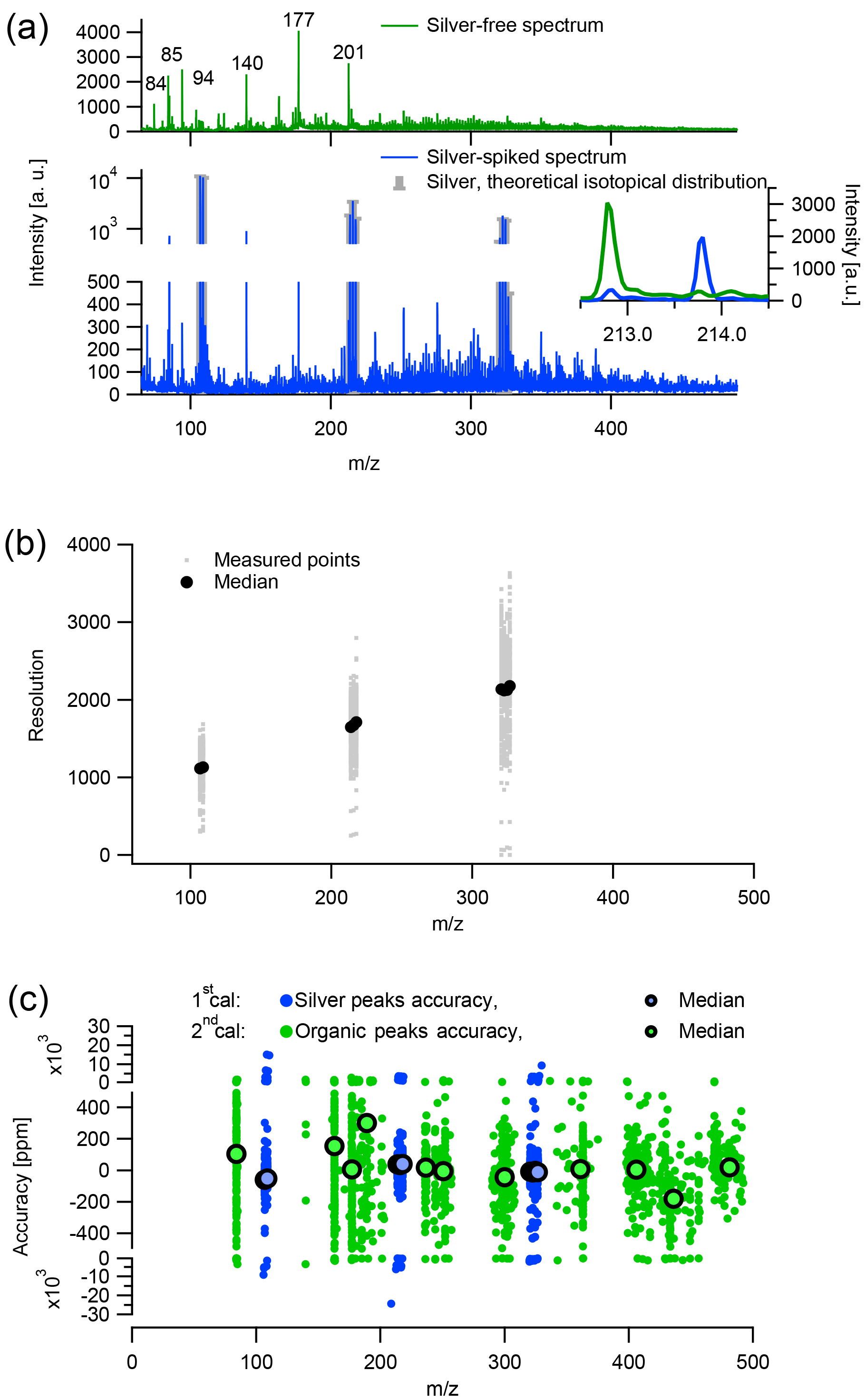
Figure 1 The m∕z calibration of LDI-MS analysis of aerosol collected on quartz-fiber filter: (a) example of calibrated silver (Ag-spec, blue) and silver-free average mass spectra (noAg-spec, green) of a filter sample. The insert in (a) displays a zoom-in of the Ag-spec and noAg-spec. (b) Operational resolution determined based on silver monomer, dimer, and trimer. Panel (c) shows m∕z calibration accuracy for both steps of the m∕z calibration.

The m∕z calibration parameters were highly variable between different samples. Therefore, to determine unit mass resolution integration regions it was necessary to perform an m∕z calibration on every single sample. However, unlike in the Aerodyne AMS (${\mathrm{N}}_{\mathrm{2}}^{+}$, ${\mathrm{O}}_{\mathrm{2}}^{+}$, W⁺), there are no dominant anchor ions present in these spectra that could be used for an m∕z calibration. In the absence of such ions, we performed a two-step calibration procedure as described in the following. Each sample was spiked with silver nitrate (AgNO₃, Sigma Aldrich, >99.8 %) as an internal standard (approach illustrated in Fig. 1). In order to avoid the suppression of the sample signal, the internal standard (aqueous solution 500 ppt to 20 ppm) was only placed (as a droplet) on a small part of the sample. The 499 spectra from all positions on the measurement grid were separated and defined as (1) silver-spiked (lower panel in Fig. 1a), (2) silver-free (upper panel in Fig. 1a), and (3) intermediate silver. Intermediate silver cases were defined using the signal intensity in the regions of the mass spectrum where silver was expected, in comparison to adjacent silver-free regions of the spectrum, and were discarded. To calculate the first calibration, we calibrated the average silver-spiked spectrum of each filter sample, using the peaks of the silver monomer (m∕z 107, 109 Th), dimer (m∕z 214, 216, 218 Th), and trimer (m∕z 321, 323, 325, 327 Th). We found that this calibration of the silver-spiked spectrum was not directly applicable to the average silver-free mass spectrum. Possibly, spiking the filter region with aqueous AgNO₃ caused enough of a change to the surface of the filter sample to influence the ionization physics. This could affect the m∕z calibration, since the delayed-pulse ion extraction in our instrument is not orthogonal to the ablation plume but nearly parallel. Therefore, a second calibration was obtained for the averaged silver-free spectra using prominent non-silver peaks present in both spectra. Such a two-step calibration is necessary to achieve accurate m∕z calibrations of the silver-free spectra.

After calibration, mass spectra were baselined using the following custom algorithm. A window of width 1 Th (the detector bins were approximately 0.04 Th in width) was applied to identify the lowest signal intensity of that range, which was defined as the baseline. The window was moved across the mass spectrum with steps of 0.25 Th to obtain a baseline spectrum. After linear interpolation, the baseline was subtracted from the spectrum. Subsequently the spectra were integrated to unit mass resolution sticks (UMR, 1 stick per unit mass). The UMR integration window was not centred at integer masses, but rather at integer mass plus the mass defect of an alkyl ion (R-${\mathrm{CH}}_{\mathrm{2}}^{+}$). The width of this window was defined as extending to the minimum signal intensity above and below the centre using the first derivative of the signal.

To enable a direct comparison of LDI-MS and HR-AMS results, the intensity of the calibrated and baseline-subtracted spectra ($I_{m/z}^{\prime }$) with arbitrary units were scaled to OA (µg m⁻³) using the respective OA contents of the filter samples (see Eq. 1, with rescaled intensities termed I_m∕z thereafter). OC_Sunset was determined using the Sunset OC ∕ EC analyser and (WSOA ∕ WSOC)_oAMS through WSOA measurements (described in Sect. 2.1, WSOC being water-soluble organic carbon). Note that an additional contribution of non-organic material to the signal could not be fully excluded. However, we consider the detected signal mainly to be related to organics based on the measurements of ambient aerosol with offline LDI-MS systems using different laser wavelengths (193 and 355 nm, Aubriet and Carré, 2010) and pure components (337 nm, Goheen et al., 1997) indicating that sulfate and nitrate respond only in the negative mode. Additionally, molecular nitrate and ammonium ions are too small to be detected in this study (cutoff at m∕z 65 Th). We also do not expect clusters between inorganic cations and organics because we did not observe significant amounts of silver/organic clusters in silver-spiked spectra (Fig. 1a).

$$\begin{array}{}\text{(1)}& {\displaystyle }{I}_{m/z}={\displaystyle \frac{I_{m/z}^{\prime }}{{\sum }_{m/z}{I}_{m/z}}}\cdot {\text{OC}}_{\text{Sunset}}\cdot {\left({\displaystyle \frac{\text{WSOA}}{\text{WSOC}}}\right)}_{\text{oAMS}}\end{array}$$

2.3 Source apportionment/PMF

2.3.1 General and input data

Positive matrix factorization (PMF, Paatero and Tapper, 1994; Paatero, 1997) is a widely used algorithm for source apportionment. PMF (Eq. 2) explains the variability in a dataset (x_i,j, here LDI-MS mass spectra scaled to OA, I_m∕z) as a linear combination of constant factor profiles (f_k,j, here mass spectral signatures) and their time-dependent contributions (g_i,k, here concentrations of this factor). The index i represents a specific point in time, j the signal at a specific m∕z, and k a factor (up to the number of factors p).

$$\begin{array}{}\text{(2)}& {\displaystyle }{\displaystyle }{x}_{i,j}=\sum _{k=\mathrm{1}}^p{g}_{i,k}{f}_{k,j}+e_{i,j}\end{array}$$

PMF is solved by minimizing the residuals e_i,j weighed by the measurement uncertainty, here ${\mathit{\sigma }}_{\text{PMF, }i,j}.$ In this study, PMF was solved by the multilinear-engine 2 (Paatero, 1999 and references therein) using the front-end user interface SoFi 4.9 (Canonaco et al., 2013) developed for Igor Pro v6 (Wavemetrics). We performed PMF without constraints of e.g. reference mass spectra of aerosol sources (unconstrained PMF). The data matrix consisted of the stick-integrated LDI-MS spectra (m∕z 65 to 485 Th scaled to OA) of all 785 filter samples. We excluded all m∕z's for which we expected silver signals (listed in Sect. 2.2.2) even though only silver-free spectra (according to the definition given above) were considered.

We determined the PMF uncertainty matrix (σ_PMF, i,j) based on the instrument repeatability (described in Sect. 3.1) according to the two-component model for measurement uncertainty described by Rocke and Lorenzato (1995) and Wilson et al. (2004). This approach ultimately means that an absolute-error term (e.g. due to noise) is combined in quadrature with a relative-error term (e.g. due to scaling or calibration uncertainties) as shown in Fig. 2 and in Eq. (3) (${\mathit{\sigma }}_{\text{PMF},m/z}^{\prime }$, for a single mass spectrum). The need for and applicability of such an error model has been demonstrated by Corbin et al. (2015) for MS-PMF. We obtained the two error terms by fitting Eq. (3) to the relative standard deviation (SD) of replicate measurements for each filter and experiment, and we applied the averaged fitted parameters to the entire dataset (constant error term, σ_abs, and an error term proportional to the measured peak intensity, $I_{m/z}^{\prime }{\mathit{\sigma }}_{\text{rel}}$).

$$\begin{array}{}\text{(3)}& {\displaystyle }{\displaystyle }{\mathit{\sigma }}_{\text{PMF, }m/z}^{\prime }={\displaystyle \frac{\sqrt{{\mathit{\sigma }}_{\text{abs}}^{\mathrm{2}}+I_{m/z}^{{}^{\prime }\mathrm{2}}{\mathit{\sigma }}_{\text{rel}}^{\mathrm{2}}}}{I_{m/z}^{\prime }}}\end{array}$$

The error was scaled to OA in the same way as the LDI-MS mass spectra (Eq. 4).

$$\begin{array}{}\text{(4)}& {\displaystyle }{\displaystyle }{\mathit{\sigma }}_{\text{PMF, }m/z}={\mathit{\sigma }}_{\text{PMF},m/z}^{\prime }\left({\displaystyle \frac{I_{m/z}}{I_{m/z}^{\prime }}}\right)\end{array}$$

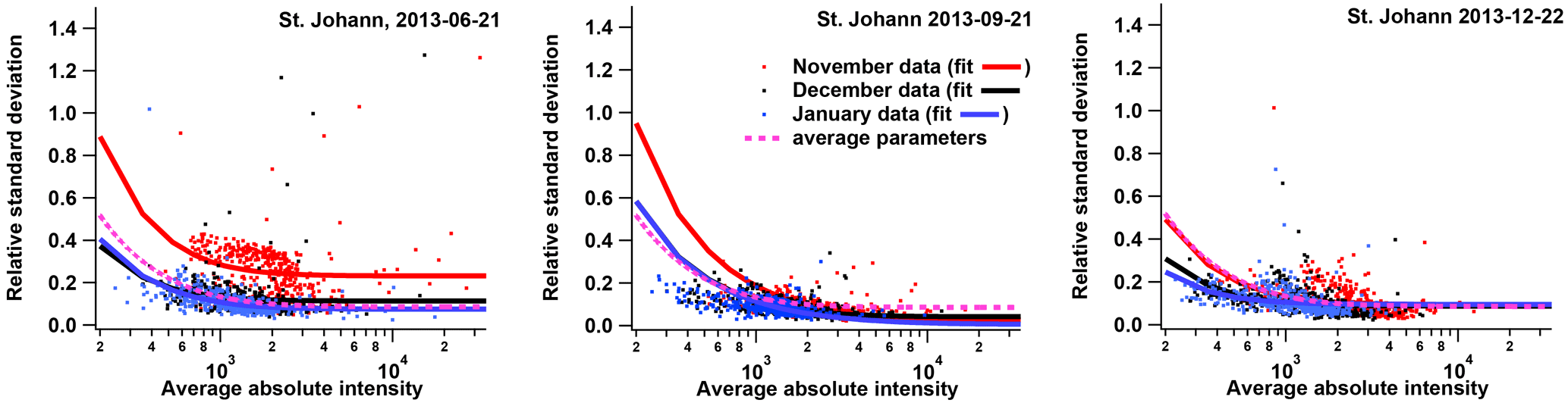
Figure 2 Error model parametrization based on three samples (Basel, 21 June, 21 September, and 22 December 2013) measured on three instances, each time with 10 repeats on one sample holder.

2.3.2 Uncertainty estimate of PMF results

A well-established statistical tool for estimating the uncertainty is the bootstrap technique, which consists of randomly resampling the input data, with replacement, to create input matrices with the same dimensions as the initial data matrix (Davison and Hinkley, 1997; Brown et al., 2015). We performed 1000 bootstrap PMF runs (also using the replicate measurements) with different initial guesses (“seeds”) using input matrices of the same size (785 filter samples and 412 ions), resulting in the uncertainty estimate σ_bs. We also assessed and parameterized the uncertainty arising from the intra-day repeatability for three filters analysed repeatedly by the LDI-MS on three different days, 10 times each day (σ_intra-day, see Supplement). The reported uncertainty for each PMF factor σ_tot is the quadratic sum of σ_bs and σ_intra-day, as explained in more detail in the Supplement. Potential long-term drifts in instrumental response were evaluated (σ_inter-day, see Fig. S10 in the Supplement) but were not accounted for numerically.

3 Results and discussion

3.1 Calibration, repeatability, and quantification

An example of a sample spectrum after m∕z calibration and baseline subtraction, separated into silver-spiked and silver-free spectra and averaged over the entire filter punch, is presented in Fig. 1a. The silver-spiked spectrum features an intensive signal at m∕z 214 Th related to the ¹⁰⁷Ag₂ dimer, in contrast to the silver-free spectrum.

The operational mass resolution, m∕Δm, based on the measurements conducted on one sample tray per month and the accuracy of both calibration steps are shown in Fig. 1b and c, respectively. The operational resolution of the instrument was only determined for the silver monomer (resolution 1100), dimer (1700), and trimer (2100) as we are confident of the absence of interfering ions for these peaks. In comparison to the LDI-MS, the HR-ToF AMS in V-mode (and W-mode) has a resolution of ca. 2000 (4000) at m∕z 100 Th and an m∕z calibration accuracy <20 ppm (<10 ppm, DeCarlo et al., 2006). With this accuracy and resolution, neither distinguishing different ions at the same nominal mass nor estimating properties such as O ∕ C and H ∕ C for a nominal mass following Stark et al. (2015) was possible for the quartz-filter LDI-MS measurements. Instead, the spectra were integrated to UMR sticks. The presence of considerable signal at odd masses might indicate that significant fragmentation occurs during desorption and ionization of the organic aerosol in the LDI-MS (Figs. 1a, 3 and 4). However, Samburova et al. (2005a) suggested that fragmentation in this instrument is negligible. The mass spectral signatures acquired in this study are similar to the ones in Samburova et al. (2005a), and the laser energy applied in this study is lower than in the former study. This suggests that also during our measurements, fragmentation was not a prominent process. Overall, the extent of fragmentation remains unclear.

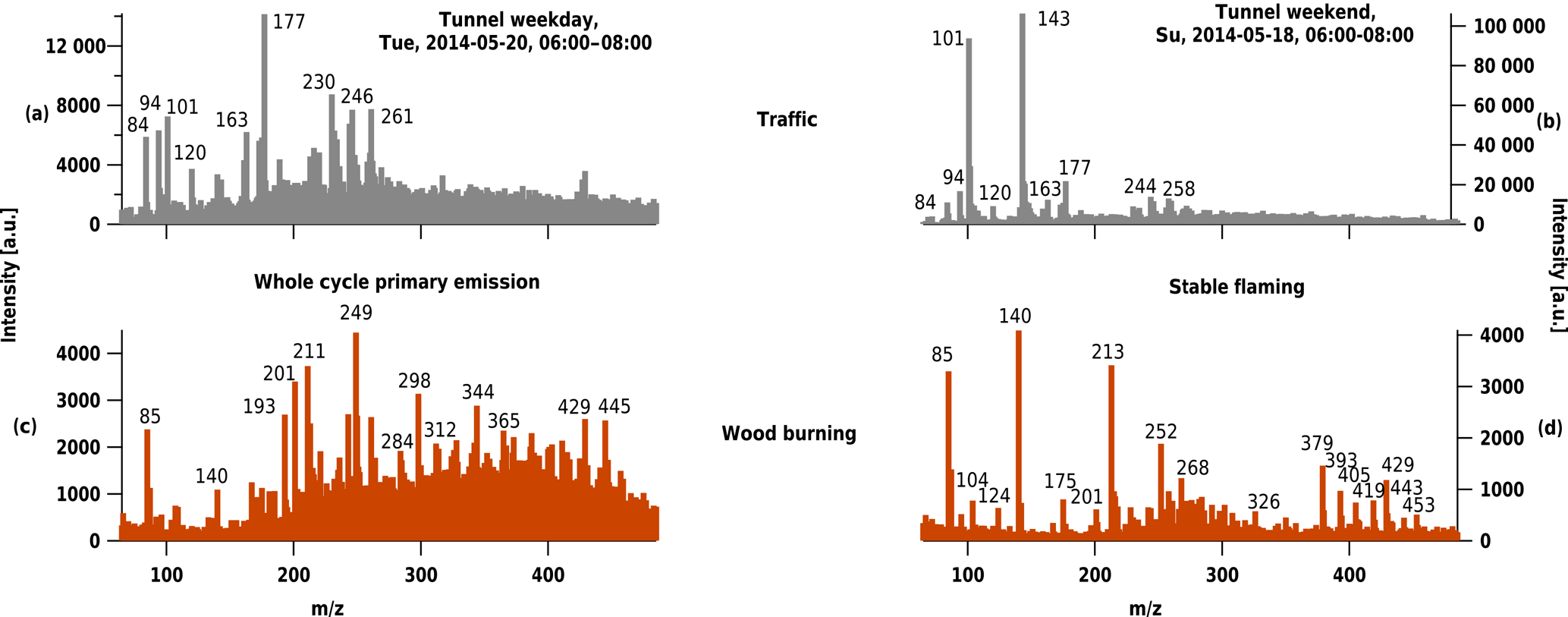
Figure 3 Samples representing different combustion sources (a) and (b) traffic emissions from samples collected in Islisberg tunnel (exit Wettswil, Switzerland), and (c) primary wood burning using whole cycle emissions (d) and stable flaming phase emissions (d). In absence of a measurable mass spectrum, no spectrum for cooking emissions is displayed.

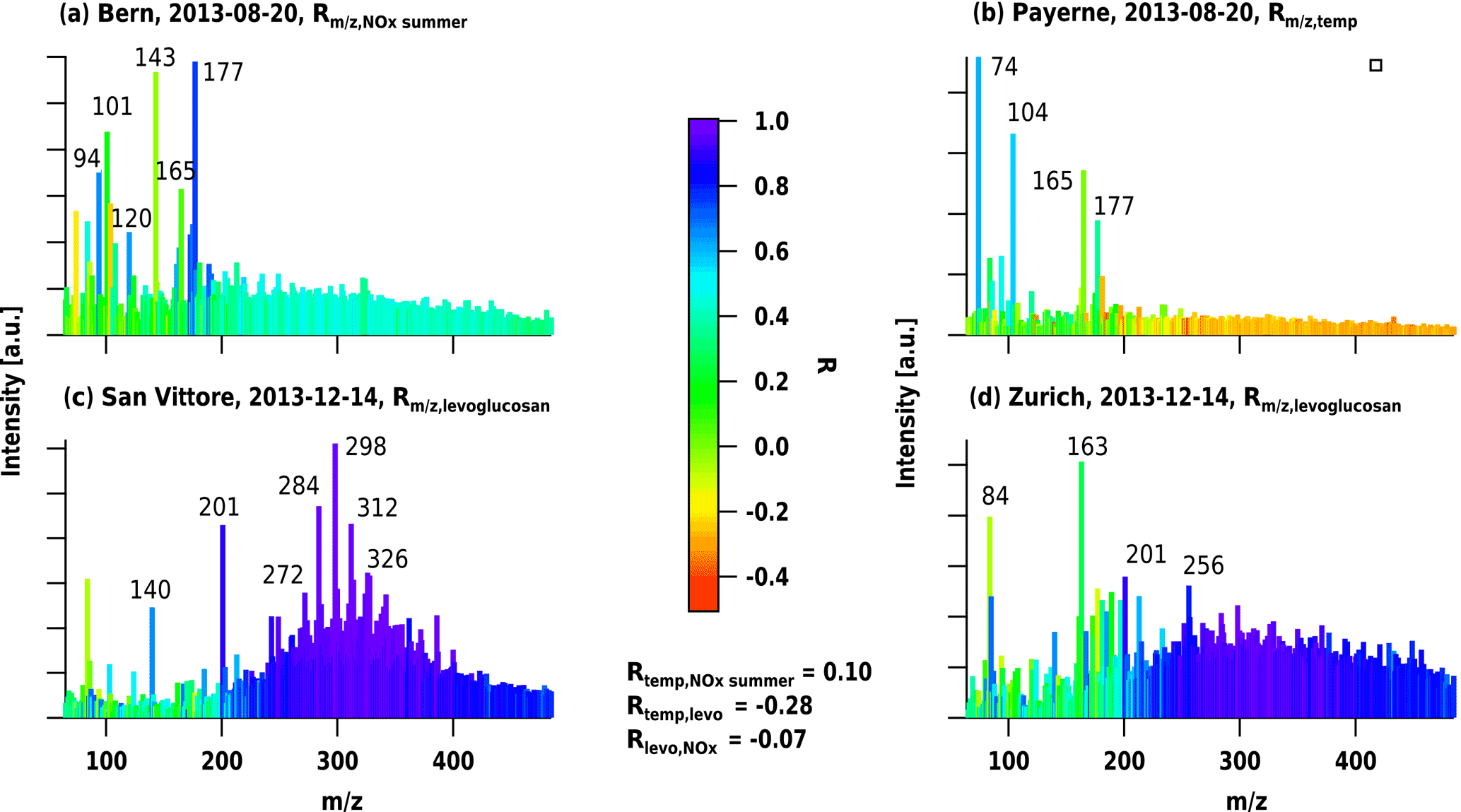
Figure 4 LDI-MS mass spectra from summer and winter samples (dates given in the legend) from a traffic-influenced site (Bern), a rural site (Payerne), a wood-burning-influenced site (San Vittore), and an urban background site (Zurich). Spectra are colour-coded, with the correlation coefficient (r) between the m∕z's and a specific environmental parameter for the whole dataset: for (a) the correlation with NO_x during summer, for (b) the correlation with temperature, and for (c) and (d) the correlation with levoglucosan.

The repeatability of the mass spectral signature was assessed in detail for three selected filters (collected in Basel on 21 June, 21 September, and 22 December 2013). Ten punches from each of these three samples were prepared on the sample holder in the same time and subsequently measured. The given procedure was repeated on three occasions (on 25 November 2015, 17 December 2015, and 28 January 2016). The relative error was related to the absolute signal intensity for each m∕z for each sample and experiment (Fig. 2), with an asymptotic value of only $\sim \mathrm{9}\pm \mathrm{7}$ % at high signals (average and SD of fitting Eq. 3). The average absolute error for small signals was 102±48 a.u. (from Eq. 3). These parameters did not show a temporal trend, which suggests that the measurements are repeatable, despite filter inhomogeneity and laser instability. Analyses of field blanks (also spiked with AgNO₃) exhibited low signal with 99 % of peaks below detection limit (defined as 3×σ_abs). The other 1 % of the peaks (m∕z 197, 249, 251, 322 324 Th) exhibited high variability among the field blank analyses (see details in Supplement, Figs. S1 and S2). Therefore, no blank subtraction was performed.

The total measured intensity $(I_{\text{tot}}=\sum I_{m/z}^{\prime })$ did not show a relation with the filter loading (OC, OC + EC, PM₁₀; see Fig. S3 in the Supplement), indicating that factors such as the composition, size, and/or mixing state of the collected aerosol particles had a larger influence on the measured ion intensities than the mass of PM. Moreover, replicate measurements indicated that the I_tot of a single sample measured on different instances was affected by an instrumental drift (details in Supplement, Fig. S4).

3.2 Combustion-source samples

Filters from cooking processes (frying, related largely to oil pyrolysis; Klein et al., 2016a; Allan et al., 2010) did not yield measurable mass spectra in our LDI-MS. This observation is in agreement with a prior study, which performed in situ single-particle LDI-MS measurements at 266 nm (using the ATOFMS) and did not observe cooking particles (Healy et al., 2013). The lack of either graphene-like black carbon or polycyclic aromatic hydrocarbons (PAHs) to absorb the LDI-MS laser may explain these observations (Healy et al., 2013), which suggests that our measurements are more sensitive towards certain PM components. We speculate that it may be possible in some cases to observe cooking-related ions in the LDI-MS of atmospheric samples, if such ions are secondary ions formed in the ablation plume or cooking particles are coated by absorbing SOA.

The mass spectra of tunnel filter samples were complex and characterized by distinct patterns (Fig. 3). Some m∕z fragments (e.g. 84, 94, 101, 177 Th) were present in the weekday and weekend tunnel samples, but not in the biomass smoke. Between the two tunnel samples, large differences could also be identified. The tunnel sample collected on a Tuesday during rush hour (06:00–08:00) showed many more peaks (among others, 163 and 177), which were less prominent during the weekend at the same time and in the same location (where m∕z 101 and 143 Th dominated the weekend spectrum).

Previous studies have identified lubrication oil as a major component of diesel- and gasoline-vehicle exhaust (Gentner et al., 2017; Chirico et al., 2011), which consists largely of aliphatic hydrocarbons. Cooking particles similarly consist of such hydrocarbons (Schauer et al., 2002; Allan et al., 2010; Crippa et al., 2013). Since we did not observe a mass spectrum for the cooking sample, but do observe one for the tunnel sample, our detection of tunnel particles may rely either on the presence of black carbon or PAHs on the filter samples. To the extent that these species are heterogeneously distributed within the sampled aerosol particles, our technique may be specifically sensitive to certain components of traffic emissions.

The mass spectrum of the wood burning sample from the whole burning cycle shows a complex pattern with a bimodal envelope of relatively intense ions from m∕z 200 Th onwards. By contrast, the sample from the stable flaming phase shows fewer peaks (e.g. m∕z 85, 140, 213 Th) with a less significant envelope of ions.

3.3 Ambient samples

Typical mass spectra from four different locations known to be heavily influenced by specific sources at different times of the year are displayed in Fig. 4. The fragments are colour-coded by their correlation coefficients with three different markers or proxies for aerosol types, i.e. NO_x for traffic exhaust (Fig. 4a), levoglucosan for biomass burning emissions (Fig. 4c and d), and temperature for SOA production (as temperature is expected to exponentially enhance biogenic emissions, Leaitch et al., 2011, Fig. 4b). In general, the mass spectra from wintertime were characterized by higher contributions from higher-molecular-weight fragments compared to summer. For the winter sample from San Vittore, a large “hump” was present, on top of which signals appeared with high intensities and a highly regular pattern of m∕z differences of 14 Th. These fragments, albeit not all detected in smog chamber biomass burning aerosols, were highly correlated with levoglucosan, a unique marker of biomass smoke.

The m∕z's of 84, 94, 101, 120, 143, 165, and 177 Th, also detected in tunnel samples, showed high relative intensities in Bern in summer, of which 94, 120, and 177 Th correlated with NO_x, which suggests a high contribution of traffic emissions at this location, consistent with previous observations (Zotter et al., 2014). These ions were also observed, but to a lesser extent, at the rural site of Payerne. At the latter site, the highest intensities were found for m∕z 74 and 104 Th. Only these two ions showed a clear relation with temperature and a clear increase during summer. Overall, this spatial and temporal variability observed in the spectral fingerprints and the correlation of specific fragments with environmental parameters suggest that LDI-MS data contain mass spectral information that may be used to separate the contribution from different aerosol sources. Source apportionment analysis using these data in combination with PMF was therefore explored in the following.

3.4 Source apportionment results

3.4.1 PMF setup

Residual analysis of preliminary PMF runs showed that structure in the residuals was removed when increasing the number of factors up to five but not when further increased. However, when allowing for seven factors, further environmentally interpretable separations could be achieved. Increasing to eight factors led to the separation of a third traffic-related factor, which however contributed little to the overall mass. Therefore, we opted for seven factors (see details in Supplement, Figs. S6, S7, and S8).

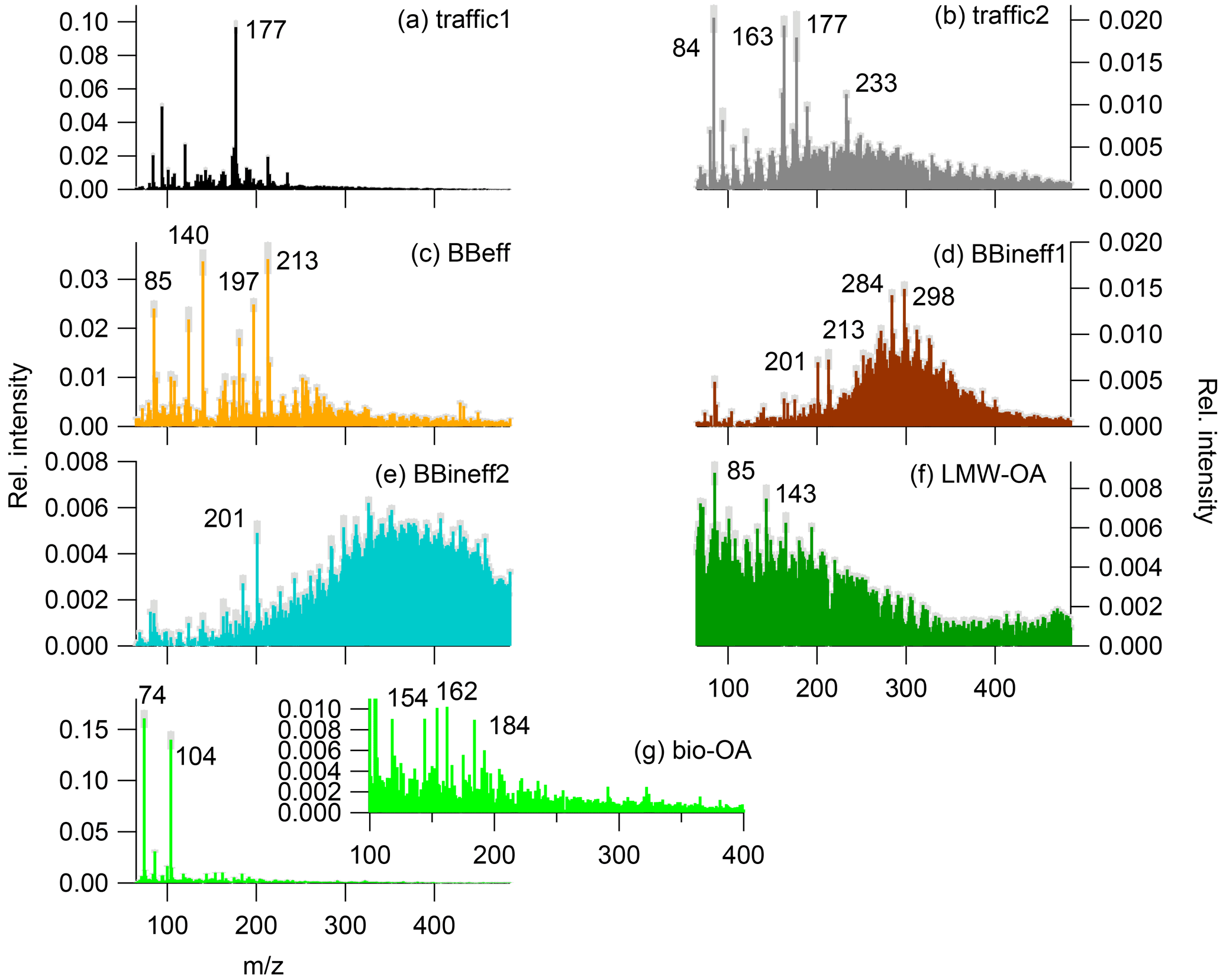
Figure 5 PMF factor profiles (coloured sticks) and their uncertainty (grey shaded areas, variability among PMF runs): (a) traffic1, (b) traffic2, (c) efficient wood burning (BBeff), (d) inefficient wood burning (BBineff1), (e) inefficient wood burning 2 (BBineff2), (f) lower-molecular-weight OA (LMW-OA), and (g) biogenic OA (bio-OA).

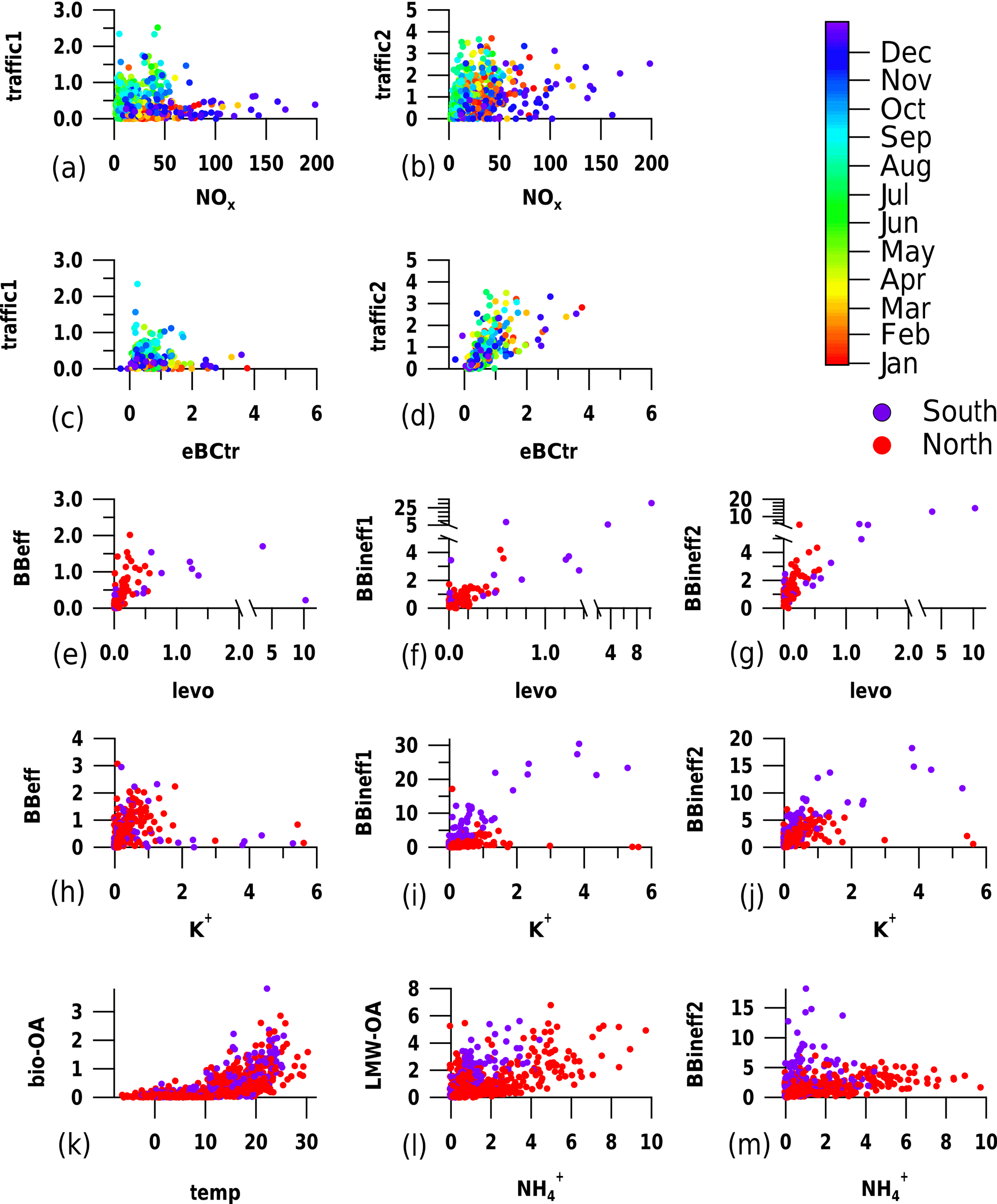
Figure 6 Scatterplots between factor time series and respective markers (traffic1, traffic2, BBeff, BBineff1, BBineff2, bio-OA, LMW-OA, eBC_tr, levoglucosan, potassium, and ammonium are displayed in µg m⁻³, NO_x in ppm, and temperature in ^∘C).

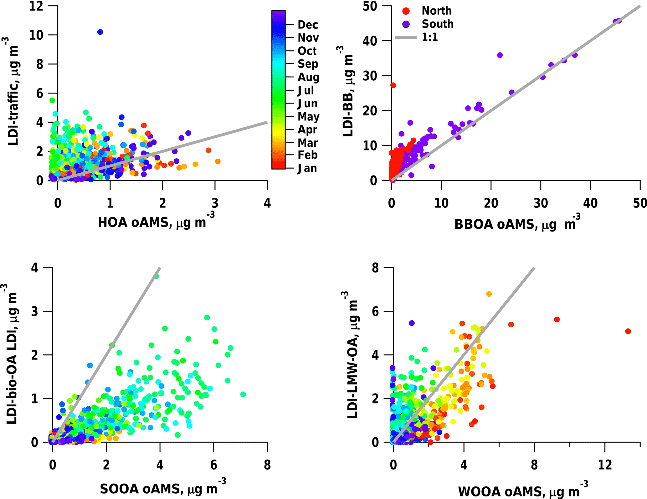
Figure 7 Comparison of the LDI-MS to reference offline AMS source apportionment results for the sum of traffic-related factors (LDI-traffic, $R_{\text{LDI, oAMS}}^{\mathrm{2}}=\mathrm{0.04}$), sum of wood-burning-related factors (LDI-BB, $R_{\text{LDI, oAMS}}^{\mathrm{2}}=\mathrm{0.83}$), bio-OA ($R_{\text{LDI, oAMS}}^{\mathrm{2}}=\mathrm{0.62}$), and LMW-OA ($R_{\text{LDI, oAMS}}^{\mathrm{2}}=\mathrm{0.45}$).

3.4.2 Interpretation of PMF factors

Traffic-related factors

Two factors could be related to traffic (Fig. 5a and b, termed traffic1 and traffic2, respectively) based on patterns in the factor profiles similar to patterns in the samples measured in the tunnel on a weekday (Fig. 3a). Since the signatures obtained from the tunnel filters represent both tailpipe exhaust and resuspended dust, the two factors identified could be a mixture of both sources. In order to elucidate the reasons behind the separation of traffic-related aerosols into two factors by PMF, we inspected their relationship with NO_x and eBC_tr, typical markers of traffic emissions. Both traffic1 and traffic2 showed increasing concentrations with increasing NO_x levels. However traffic1 ∕ NO_x and traffic2 ∕ NO_x were seasonally variable ($R_{p,\text{traffic1},{\text{NO}}_x}=-\mathrm{0.17}$, $R_{p,\text{traffic2},{\text{NO}}_x}=\mathrm{0.24}$, Figs. 6 and S9). While traffic2 correlated with eBC_tr, traffic1 did not show such a dependency (Table S1, Figs. 6 and S9). The correlation with eBC_tr suggests that traffic2 is related to primary emissions from the combustion process. Based on the lack of correlation between traffic1 and eBC_tr, traffic1 might also be influenced by other processes, such as e.g. secondary production. Additionally, tailpipe exhaust cannot be distinguished from other traffic-related emissions in the tunnel samples and might also contribute to traffic1.

The ratio of both factors to NO_x exhibited a clear seasonality, increasing during summer (Fig. 6a and b). Such a change can either be caused by a change in the emission patterns, by an enhanced photochemical production of these factors, or due to a change in the lifetime of e.g. NO_x. In Fig. 6c and d, we compared the contribution of the traffic-related factors with those of eBC_tr, another tracer of traffic emissions whose lifetime is similar to OA (see Fig. S9 for summer points only). The comparison shows that while the ratio of traffic2 to eBC_tr is not season-dependent, the one of traffic1 to eBC_tr increases during summer. The seasonal variability in the relative contribution of traffic1 might thus be related to a seasonal change in fleet composition or combustion conditions, or an enhancement of the photochemical production of this fraction. An enhanced dust resuspension in the warm season (e.g. more dust on the road due to less precipitation) could also contribute to an increased traffic1 concentration in summer.

Wood-burning-related factors

Three factors could be related to wood burning emissions (Fig. 5c, d and e). The first (Fig. 5c) showed a similar mass spectral pattern to samples from laboratory experiments from stable flaming wood burning exhaust from a log wood burner and thus was termed efficient wood burning (BBeff). The fingerprint of the second (Fig. 5d) resembled that of laboratory wood smoke aerosols from the entire burning cycle including the inefficient starting and burnout phase and, therefore, was related to inefficient wood burning (BBineff1). BBineff1 showed also a similar signature as spectra from wood burning haze episodes in San Vittore identified by high levoglucosan concentrations. The third (Fig. 5e) mostly explained the masses above m∕z 300 Th. The signature of the whole cycle wood burning aerosols from a log wood burner (Fig. 3c) also showed high relative contributions at high m∕z, similar to this factor. For this reason this factor was termed BBineff2. Both BBeff and BBineff1 correlated with levoglucosan (Fig. 6e and f, Table S1). Similar to BBeff and BBineff1, BBineff2 correlated with levoglucosan and thus could be related to wood burning emissions (Fig. 6g, Table S1). However, BBineff2 also correlated with ${\mathrm{NH}}_{\mathrm{4}}^{+}$, a marker of aged aerosols, at the northern sites (Fig. 6m), which may also indicate that this fraction can include aged and/or secondary components (Table S1).

Comparing the wood-burning-related factor time series to potassium (K⁺), an inorganic wood burning marker, mostly present in ash, provides further insight into the separation of the three wood-burning-related factors. Among the factors related to wood burning emissions, BBeff has a lower $\text{BB}/{\mathrm{K}}^{+}$ ratio (2.4, IQR 1.25–4.2) than BBineff1 (6.0, IQR 2.7–12.0) and BBineff2 (11.6, IQR 6.0–21.0). In wood burning experiments, it was found that OC, EC, PM₁₀, and PAH emissions increase relative to the potassium output during non-ideal burning conditions (Lamberg et al., 2011). Zotter et al. (2014) found a north–south gradient in $\text{levoglucosan}/{\mathrm{K}}^{+}$ and ${\mathrm{OC}}_{\text{nf}}/{\mathrm{K}}^{+}$ in Switzerland and hypothesized that it might be linked to the burning conditions. Thus the higher the LDI-BB ∕ K⁺ ratios (north: 16.6, IQR 10.4–30.8 south: 30.8, IQR 22.5–44.2), the less efficient the burning conditions are, which in turn supports the hypothesis that BBeff represents the most efficient burning conditions among the three factors. All wood-burning-related factors showed higher median $\text{BB}/{\mathrm{K}}^{+}$ ratios at the southern Alpine valley site (BBeff: 3.0 with IQR 1.1–5.2, BBineff1: 10.9 with IQR 7.5–17.3, BBineff2: 15.8 with IQR 9.9–24.0) than in northern Switzerland (BBeff: 2.1 with IQR 1.2–3.4, BBineff1: 4.3 with IQR 2.2–8.6, BBineff2: 9.6 with IQR 5.2–18.3), as also visible in Fig. 6h, i and j. The north–south gradient in the $\text{BB}/{\mathrm{K}}^{+}$ ratios might be caused by imperfections of the separation of the burning conditions by PMF, but other effects such as the age of the stove population and the technology used could contribute as well. The wood consumption (BFE, 2013) of automatic burners (> 50 kW), was higher in northern Switzerland (in the respective regions, 48 m³ wood km⁻² area) than in southern Switzerland (8 m³ wood km⁻² area). Since the OA, POA, and SOA emissions of pellet burners during the stable phase are drastically reduced compared to modern log wood burners in a stable flaming phase (e.g. Heringa et al., 2011), they might contribute overproportionately to potassium in northern Switzerland but only little to OA, leading to the higher BB ∕ K⁺ ratios at the southern Alpine sites.

Biogenic-OA, low-molecular-weight OA, and other OA factors

A factor characterized by high contributions of low-molecular-weight ions (Fig. 5f, LMW-OA) correlates with ${\mathrm{NH}}_{\mathrm{4}}^{+}$, suggesting secondary processes as origin (Fig. 6l, Table S1). At the southern Alpine valley sites, the $\text{LMW-OA}/{\mathrm{NH}}_{\mathrm{4}}^{+}$ ratio was higher than in northern Switzerland. As ${\mathrm{NH}}_{\mathrm{4}}^{+}$ is mostly associated with the secondary inorganic species sulfate and nitrate, this variability will mostly be related to differences in the volatile organic compounds (VOCs) vs. SO₂ and NO_x emissions, along with temperature differences influencing the partitioning of nitrate to the particle phase.

The contribution of the last remaining factor showed an exponential increase with temperature, similar to terpene emissions and biogenic SOA (Leaitch et al., 2011), suggesting this factor to be strongly influenced by biogenic SOA production. Therefore, this factor was termed bio-OA. The relationship between bio-OA and temperature was similar both at the northern and southern sites (Fig. 6k, Table S1 in the Supplement). The bio-OA had a highest relative contribution at the most rural site in the dataset (Payerne: yearly average bio-OA 11 %, yearly average NOx concentration: 9 ppb) and the lowest at the most trafficated site (Zurich: yearly average bio-OA 3 %, yearly average NOx concentration: 48 ppb). The chemical signature of bio-OA was dominated by fragments at m∕z 74 and 104 Th (Fig. 5g). The nature of these fragments remained unidentified, but could not be related to monoterpene or sesquiterpene SOA because of their very low m∕z. Further, the composition of secondary aerosols is expected to be much more complex, showing a series of fragments distributed over a wide m∕z range. We note that the abundance of the fragments at m∕z 74 and 104 Th relative to the total signal should not be directly related to their absolute concentrations, and their ionization efficiency might be superior to that of other molecules, which may increase their apparent contribution.

3.4.3 Comparison to offline AMS and assessment of LDI-MS response factors

The LDI-MS source apportionment results were compared to those based on offline AMS (oAMS) analyses performed on the same samples (Daellenbach et al., 2017). We note that this comparison is not straightforward as different sources are separated by the two methods. For this purpose traffic1 and traffic2 were summed up to LDI-traffic, and BBeff, BBineff1, and BBineff2 to LDI-BB (Fig. 7).

As was the case for the comparison to NO_x and eBC_tr (Sect. 3.4.2), also in the comparison to the offline AMS traffic (HOA), a higher LDI-traffic/HOA was observed in summer, which contributes to the low correlation coefficient (R²=0.04). This might be related to the fact that HOA is only primary without major contributions of traffic SOA or dust resuspension, while LDI-traffic is potentially also influenced by aged/secondary traffic aerosol and resuspension. In contrast to summer, we observe a good agreement between LDI-traffic and HOA in winter. Thus even though a varying relative response factor (rRF) of the LDI-MS might contribute to these differences, these biases are not systematic but season-dependent. As stated earlier, LDI-traffic is thought to be a mixture of primary tailpipe exhaust, aged/secondary tailpipe exhaust, and resuspended dust (as well as tyre break and engine wear). This will be further elucidated in Sect. 3.4.5.

LDI-BB was highly correlated with offline AMS-BBOA (R²=0.83); yet the LDI-BB concentrations were higher than BBOA from oAMS, especially in northern Switzerland (with an LDI-BB : AMS-BBOA ratio between 1.4 and 4.1 for the different sites). A possible reason is also the mixing of secondary components into LDI-BB here when comparing to primary BBOA from oAMS. However, we cannot exclude that this effect is due to different rRFs of the LDI-MS for different compound classes.

The identified secondary components, LMW-OA (R²=0.45) and bio-OA (R²=0.62), also correlate with the corresponding OOA factors from the oAMS analysis, WOOA and SOOA; yet the correlation coefficients are smaller than for LDI-BB and BBOA. For these factors, differences between the two methodologies could be related to differences in the PMF performance or to differences in the response factors for different components in the LDI-MS (the LMW-OA: WOOA ratio is between 0.7 and 1.1 and the bio-OA: SOOA ratio between 0.2 and 0.4).

At some of the sites analysed with the LDI-MS in this study, OA was monitored in previous years with state-of-the-art online aerosol mass spectrometry (AMS or ACSM). Earlier campaigns with quantitative online AMS analyses show a higher SOA contribution at those sites: e.g. in Zurich, July 2005 (66 % vs. 25 % for LDI-MS summer) and December 2005 (55 % vs. 14 % for LDI-MS winter), in Roveredo (close to San Vittore), March 2005 (53 % vs. 46 % for LDI-MS summer) and December 2005 (43 % vs. 11 % for LDI-MS winter), and in Payerne, July 2005 (94 % vs. 47 % for LDI-MS summer) and December 2005 (71 % vs. 20 % for LDI-MS winter) (Lanz et al., 2010). Canonaco et al. (2013) presented source apportionment results for the winter of 2011 and 2012 for Zurich (PM₁ ACSM), also with higher SOA contributions (71 %) than the LDI-MS in 2013 (20 %).

Overall, the source apportionment results based on LDI-MS data provide source separations with similar temporal behaviours as offline AMS and online AMS and ACSM analysis; yet the results seem to overestimate combustion-related primary particle sources and underestimate secondary OA. However, we assume for this comparison that all factors give an equal response at a given concentration, i.e. the relative response factor (rRF_LDI) of all factors to be 1. The relative contribution of a factor k to the total signal observed with the LDI-MS $\left(r_{i,k,\text{LDI}}\right)$ for a specific measurement (i) depends on the factor concentration ($g_{i,k,\text{LDI}}$) as well as the sum of all factors $\left({\sum }_k^p\right(g_{i,k,\text{LDI}}\left)\right)$ separated for the LDI-MS data. Assuming that differences between the LDI-PMF and the AMS-PMF arise solely from different rRF_LDIs for different factors, $r_{i,k,\text{LDI}}$ is a function of the AMS factor concentrations $(g_{i,k,\text{AMS}}$) and the rRF_LDI of this factor:

$$\begin{array}{}\text{(5)}& {\displaystyle }{r}_{i,k,\text{LDI}}={\displaystyle \frac{g_{i,k,\text{LDI}}}{{\sum }_k^p\left(g_{i,k,\text{LDI}}\right)}}={\displaystyle \frac{g_{i,k,\text{AMS}}\cdot {\text{rRF}}_{k,\text{LDI}}}{{\sum }_k^p(g_{i,k,\text{AMS}}\cdot {\text{rRF}}_{k,\text{LDI}})}}.\end{array}$$

In order to determine rRF_LDI (Table 1) for the LDI-MS, several strong assumptions are required: (1) the sum of traffic1 and traffic2 represents HOA, (2) the sum of BBeff, BBineff1, and BBineff2 represents BBOA, (3) LMW-OA represents WOOA, (4) bio-OA represents SOOA, and (5) the AMS factors for which there is an LDI-MS equivalent, (1)–(4), are the only contributors to OA. In scenario 1, all the above assumptions are considered to be true. For scenario 1, we estimate rRF_LDI-BB as 1.84, rRF_LDI-LMW-OA as 0.29 and rRF_LDI-bio-OA as 0.40 (using LDI-traffic as reference factor, rRF_LDI-traffic=1.00). The LDI-MS factor concentrations corrected using rRF_LDI show a close relation to the uncorrected LDI factor concentrations ($R_{\text{LDI-traffic}}^{\mathrm{2}}=\mathrm{0.78}$, $R_{\text{LDI-BB}}^{\mathrm{2}}=\mathrm{0.94}$, $R_{\text{LDI-LMW-OA}}^{\mathrm{2}}=\mathrm{0.80}$, $R_{\text{LDI-bio-OA}}^{\mathrm{2}}=\mathrm{0.85}$, Fig. 8).

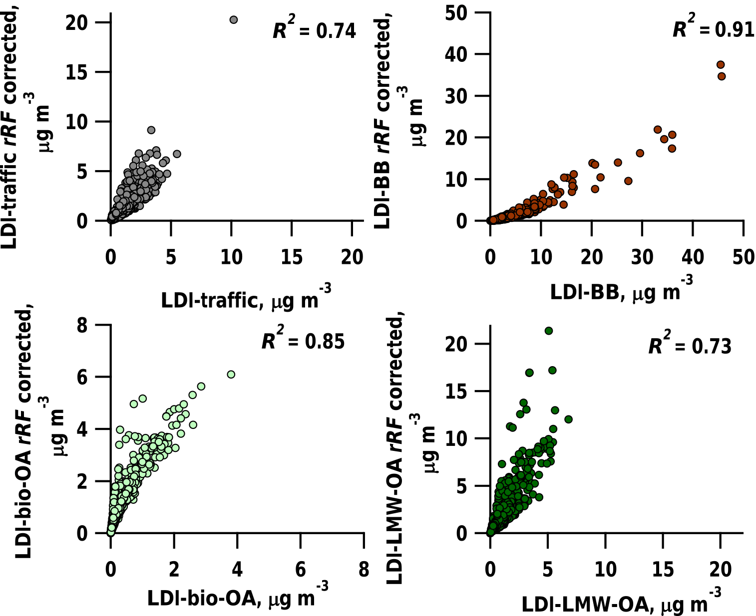
Figure 8 Comparison of LDI-MS factor concentrations corrected using relative response factors (rRF) to uncorrected LDI factor concentrations (scenario 1).

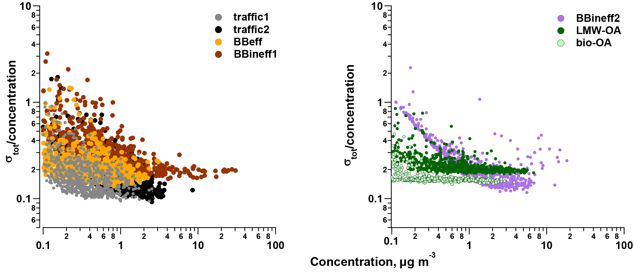
Figure 9 Relative σ_tot for the different PMF factors as a function of the factor concentration.

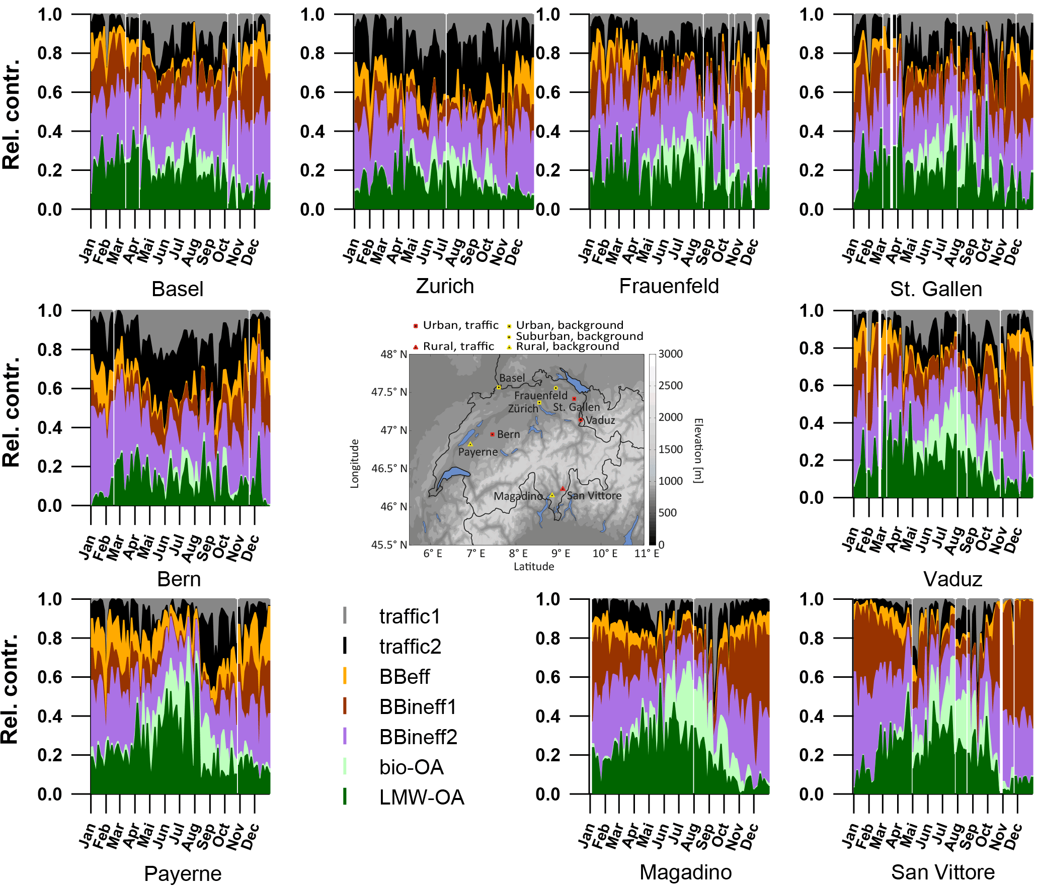
Figure 10 Relative factor time series of seven identified factors for all nine sites in the study area.

We tested the sensitivity of the rRF_LDI estimates to the assumptions (1) and (2) being wrong (scenario 2) and only assumption (5) being wrong (scenario 3). In scenario 2, we alter scenario 1 by comparing the sum of traffic1 and bio-OA to SOOA and the sum of BBineff2 and LMW-OA to WOOA when computing rRF_LDI. For scenario 2, LDI-MS factor concentrations corrected using rRF_LDI also show a close relation to uncorrected LDI-MS factor concentrations ($R_{\text{LDI-traffic2}}^{\mathrm{2}}=\mathrm{0.96}$, $R_{\text{BBeff}+\text{BBineff1}}^{\mathrm{2}}=\mathrm{1.00}$, $R_{\text{LDI-BBineff2}+\text{LMW-OA}}^{\mathrm{2}}=\mathrm{0.99}$, $R_{\text{traffic1}+\text{bio-OA}}^{\mathrm{2}}=\mathrm{0.96}$). In scenario 3, we alter scenario 1 by also considering AMS factors without an equivalent in the LDI-MS PMF. Therefore, we compare LDI-traffic to the sum of HOA, COA (cooking organic aerosol), and SC-OA (sulfur-containing organic aerosol). Under these conditions LDI-MS factor concentrations corrected using rRF_LDI show a close relation to uncorrected LDI-MS factor concentrations ($R_{\text{LDI-traffic}}^{\mathrm{2}}=\mathrm{0.75}$, $R_{\text{LDI-BB}}^{\mathrm{2}}=\mathrm{0.90}$, $R_{\text{LMW-OA}}^{\mathrm{2}}=\mathrm{0.74}$, $R_{\text{bio-OA}}^{\mathrm{2}}=\mathrm{0.85}$). The differences in rRF_LDI between scenarios 1, 2, and 3 highlight the uncertainties caused by plausible violations of the underlying assumption when determining rRF_LDI. Overall the estimates rRF_LDI are highly uncertain and their accurate determination needs to be the focus of future work. Given the high uncertainty of rRF_LDI and the good correlation between rRF_LDI corrected and uncorrected LDI-MS factor concentrations, we present uncorrected results without considering rRF_LDI.

3.4.4 Uncertainty of PMF results

The uncertainty estimate, σ_tot, includes both the statistical uncertainty (σ_bs) and the uncertainty arising from the intra-day variability of the measurements (σ_intrad; see Fig. 9, Sect. 2.3.2, and Supplement). In order to assess the impact of the intra-day variability consideration (σ_intrad) in estimating the uncertainty besides the statistical uncertainty obtained from the bootstrapping approach (σ_bs), we compared the ratios σ_bs ∕ σ_tot for the different factors: for traffic1 the ratio was 0.83, for traffic2 0.75, for BBeff 0.86, for BBineff1 0.80, for BBineff2 0.72, for LMW-OA 0.68, and for bio-OA 0.68. Thus, it was important to propagate σ_intrad. The relative uncertainties for the median factor concentrations ranged within 0.15 (for traffic1), 0.16 (bio-OA), 0.17 (LMW-OA), 0.18 (BBineff2), 0.20 (traffic2), 0.22 (BBeff, and 0.28 (BBineff1). Unlike the relative error of σ_tot of traffic1 (0.63 at the 10th percentile concentration and 0.13 at the 90th percentile concentration), traffic2 (0.68 and 0.11), BBeff (0.55 and 0.18), BBineff1 (0.47 and 0.20), BBineff2 (0.37 and 0.14), and LMW-OA (0.27 and 0.16), the relative error of bio-OA (0.20 and 0.15) only depended weakly on the factor concentration.

Table 1 Relative response factors (rRF) for LDI-MS analyses for three different scenarios.

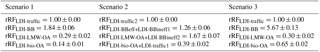
Table 2 Yearly averages of the relative factor contributions and NOx concentrations.

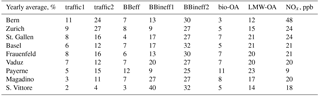
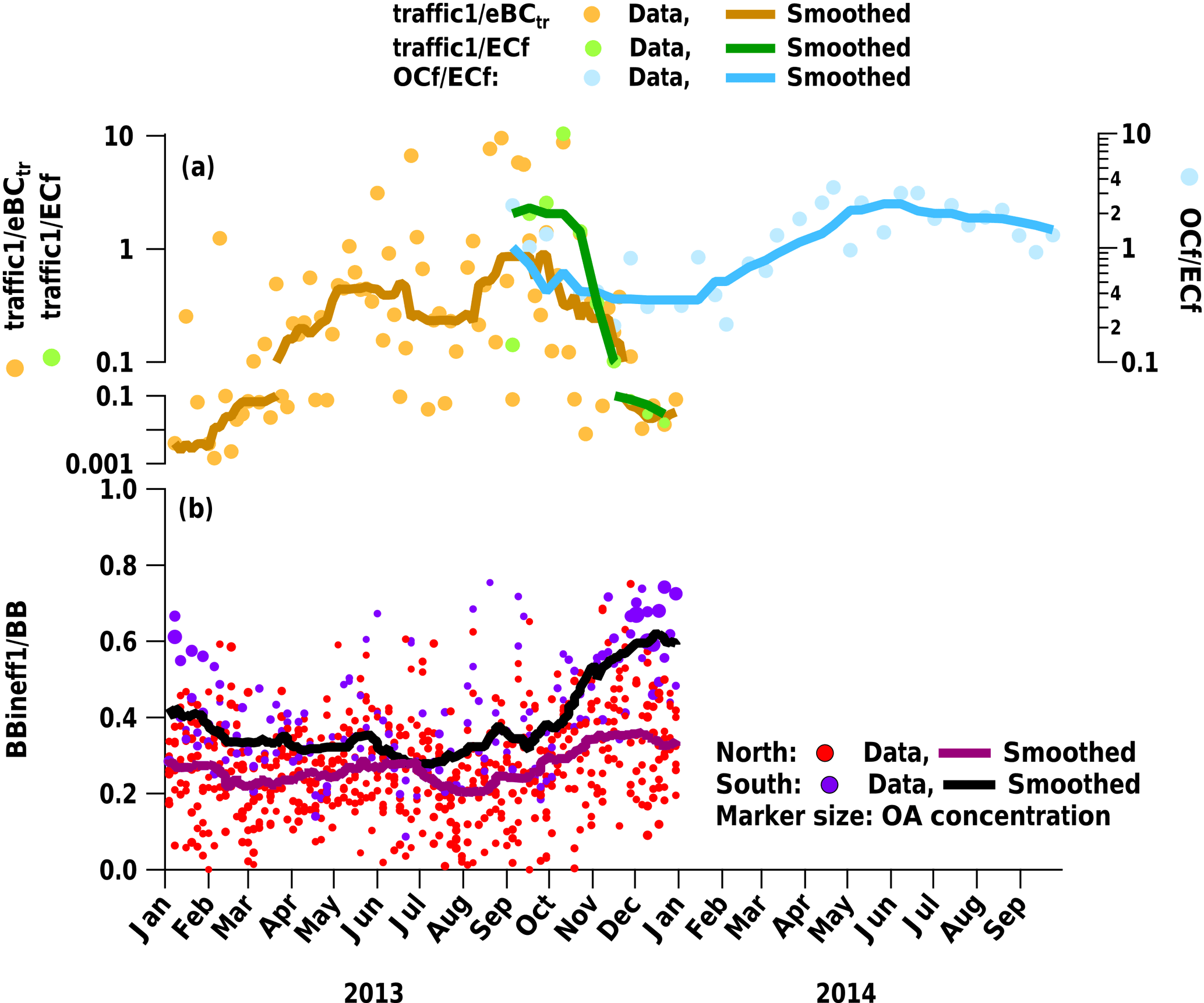
Figure 11 (a) Time series of traffic1 normalized to eBC_tr and EC_f in comparison to OC_f ∕ EC_f in Magadino and (b) influence of inefficient wood burning emissions (BBineff1) in comparison to the sum of wood-burning-influenced factors (BB = BBineff1 + BBineff2 + BBeff) for the entire dataset.

Throughout the measurement campaign, subsets of filters were analysed repeatedly in order to assess the repeatability over longer time periods (see details in Supplement, Fig. S10). Most factors did not show significant changes of the attributed concentration during the measurement campaign. However, BBeff showed decreasing and LMW-OA increasing concentrations as a function of the measurement time. This could suggest an uncertain separation of these two factors. However, for these long time delays the variability increased and only few samples were repeated with such long time delays. Furthermore, the intra-day variance largely explains the total variance (traffic1 97 %, traffic2 94 %, BBeff 85 %, BBineff1 89 %, BBineff2 82 %, LMW-OA 79 %, bio-OA 97 %, details in Fig. S10).

3.4.5 Factor variabilities and contributions

The time series of all factors are shown for the nine sites in Fig. 10 as relative contributions to OA and summarized as yearly averages in Table 2. In the yearly average for all sites, traffic1 contributes 7 %, traffic2 12 %, BBeff 7 %, BBineff1 17 %, BBineff2 32 %, LMW-OA 21 %, and bio-OA 5 % to OA as measured by the LDI-MS.

At the southern Alpine Swiss sites, the wood-burning-influenced categories (BB = BBeff + BBineff1 + BBineff2) contribute more than at the northern sites (70 % vs. 50 %). Moreover, in winter, BB explains 81 and 61 % of OA in the south and the north, respectively. This difference is mostly caused by the higher relative contribution of BBineff1 (34 % in the south vs. 14 % in the north) since BBineff2 (28 and 30 %) and BBeff (7 and 5 %) do not show strong geographical differences. The ratio BBineff1 ∕ BB (Fig. 11b) shows enhanced contributions of BBineff1 at the southern Alpine sites, especially during high pollution episodes in winter. This suggests different wood burning regimes in the two regions, as already discussed above.

After scaling of the mass spectra to OA, absolute factor concentrations still have to be interpreted with caution. One reason for this is that the relative response factors of the sources/factors are not known; another is that certain species (in analogy to the cooking-aerosol sample) may not be detected by the LDI-MS if externally mixed. In support of the quantitative interpretation of our results, we note that the sum of the wood burning related LDI-MS factors correlates well with the offline AMS counterpart ($R_{\text{LDI, oAMS}}^{\mathrm{2}}=\mathrm{0.82}$, described in Sect. 3.4.3). A yearly average of 24 % of the measured OA is apportioned to secondary OA. In summer, a bigger fraction is attributed to secondary OA (35 % compared to 16 % in winter). A total of 35 % (summer) and 1 % (winter) of the secondary OA is attributed to biogenic sources. For some samples from the same period in Magadino, the fossil and non-fossil content of OC and EC was also determined (Vlachou et al., 2017) based on the method of Zhang et al. (2012). Vlachou et al. (2017) observed increased OC_f ∕ EC_f ratios in summer, which suggests different fossil POA sources in summer than in winter, or secondary formation of fossil OA. The higher traffic1 ∕ eBC_tr and traffic1 ∕ EC_f ratios in summer are in agreement with enhanced OC_f / EC_f ratios (Fig. 11a). However, a part of traffic can also be mixed into BB, leading to an underestimation of the traffic concentrations in winter. Overall this suggests that traffic1 represents aged or secondary traffic OA.

4 Summary and conclusion

In this study, we advanced a known method for the chemical characterization of particulate matter collected on quartz-fiber filters by an LDI-MS and applied the method to 819 samples. The method included the use of silver nitrate for m∕z calibration and the automated peak integration of the mass spectra at unit-mass resolution. The benefit of LDI-MS measurements for the chemical characterization and a better understanding of the sources contributing to the ambient PM₁₀ was assessed at nine sites in central Europe throughout the entire year of 2013.

Wood combustion smog chamber experiments revealed an influence of the burning conditions on the mass spectral signature. Tunnel samples used as a reference for traffic-related emissions show mass spectral signatures distinctly different from wood combustion. Key m∕z's identified in the wood burning and traffic signatures showed links to expected markers as e.g. levoglucosan and NO_x, respectively. The ambient mass spectral information was further used for source apportionment by PMF. Therefore, the influence of efficient and inefficient wood burning was separated. The extracted wood burning emissions correlated with the results from offline AMS source apportionment. Other components are more difficult to compare quantitatively because of different source separations in PMF as well as differences in the relative response factors (rRF) of OA components. rRF determined in this study are uncertain and, therefore, not used for correcting the LDI-PMF results. The influence of traffic emissions was represented by two factors. One of these could clearly be linked to BC-related traffic (eBC_tr) and NO_x, and thus to primary emissions. The other, when normalized to eBC_tr, showed a similar behaviour to OC_f ∕ EC_f, and was therefore attributed to aged/secondary traffic OA. A factor was attributed to biogenic SOA based on its concentration exponentially increasing with temperature. Another OA factor was characterized by low-molecular-weight ions and was correlated with ${\mathrm{NH}}_{\mathrm{4}}^{+}$ and was attributed to SOA from an unknown source.