the Creative Commons Attribution 4.0 License.
the Creative Commons Attribution 4.0 License.
 | 18 Dec 2018
Characterization of ozone deposition to a mixed oak–hornbeam forest – flux measurements at five levels above and inside the canopy and their interactions with nitric oxide
Angelo Finco
Mhairi Coyle
Eiko Nemitz
Riccardo Marzuoli
Maria Chiesa
Benjamin Loubet
Silvano Fares
Eugenio Diaz-Pines
Rainer Gasche
A 1-month field campaign of ozone (O3) flux measurements along a five-level vertical profile above, inside and below the canopy was run in a mature broadleaf forest of the Po Valley, northern Italy. The study aimed to characterize O3 flux dynamics and their interactions with nitrogen oxides (NOx) fluxes from the forest soil and the atmosphere above the canopy. Ozone fluxes measured at the levels above the canopy were in good agreement, thus confirming the validity of the constant flux hypothesis, while below-canopy O3 fluxes were lower than above. However, at the upper canopy edge O3 fluxes were surprisingly higher than above during the morning hours. This was attributed to a chemical O3 sink due to a reaction with the nitric oxide (NO) emitted from soil and deposited from the atmosphere, thus converging at the top of the canopy. Moreover, this mechanism was favored by the morning coupling between the forest and the atmosphere, while in the afternoon the fluxes at the upper canopy edge became similar to those of the levels above as a consequence of the in-canopy stratification. Nearly 80 % of the O3 deposited to the forest ecosystem was removed by the canopy by stomatal deposition, dry deposition on physical surfaces and by ambient chemistry reactions (33.3 % by the upper canopy layer and 46.3 % by the lower canopy layer). Only a minor part of O3 was removed by the understorey vegetation and the soil surface (2 %), while the remaining 18.2 % was consumed by chemical reaction with NO emitted from soil. The collected data could be used to improve the O3 risk assessment for forests and to test the predicting capability of O3 deposition models. Moreover, these data could help multilayer canopy models to separate the influence of ambient chemistry vs. O3 dry deposition on the observed fluxes.
- Article
(3246 KB) - Full-text XML
-
Supplement
(1007 KB) - BibTeX
- EndNote


Ozone (O3) has been widely documented as one of the most dangerous pollutants for plants (Wittig et al., 2009; Matyssek et al., 2012; Gerosa et al., 2015; Marzuoli et al., 2018). The deposition of O3 on forest ecosystems has been extensively studied over the last 20 years with eddy covariance field campaigns (Padro, 1996; Cieslik, 1998; Lamaud et al., 2002; Mikkelsen et al., 2004; Gerosa et al., 2005, 2009a, b; Launiainen et al., 2013), which were made possible thanks also to the development of fast O3 analyzers. Measurements carried out in the 1990s were usually short-term field campaigns, while more recent campaigns have extended the observation periods and therefore led to a better understanding of the processes controlling O3 deposition (Mikkelsen et al., 2004; Gerosa et al., 2005; Fowler et al., 2009; Rannik et al., 2012; Zona et al., 2014; Fares et al., 2010, 2012, 2014; Clifton et al., 2017; Finco et al., 2017).
These studies highlighted that an important deposition pathway is represented by the O3 uptake by trees through leaf stomata. The O3 amount entering the stomata strongly depends on the environmental and physiological factors that drive stomata opening (Jarvis, 1976; Emberson et al., 2000), such as, for example, the soil water availability that is positively correlated to the stomatal O3 flux (Gerosa et al., 2009a; Büker et al., 2012).
Ozone deposition pathways other than plant stomata are usually grouped as nonstomatal deposition, although they include merely physical dry deposition processes and chemical consumption processes due to ambient air chemistry. Among these processes, which still remain to be understood in depth, we find the thermal decomposition on dry surfaces (Cape et al., 2009), the deposition on wet surfaces (Fuentes et al., 1992; Altimir et al., 2004, 2006; Gerosa et al., 2009b), the deposition on soil (Stella et al., 2011), reactions stimulated by light (Coe et al., 1995; Fowler et al., 2001), chemical reactions with NO (Dorsey et al., 2004; Rummel et al., 2007; Pilegaard, 2001; Gerosa et al., 2009b) and chemical reactions with biogenic volatile organic compounds (BVOCs) (Fares et al., 2010; Goldstein et al., 2004).
Also, O3 deposition dynamics below the forest canopy and their relationship with the above-canopy O3 fluxes are still to be fully understood, since only a few studies have directly measured O3 fluxes below the canopy. For example, Launiainen et al. (2013) and Fares et al. (2014) used these measurements to assess different deposition pathways and to validate O3 deposition models, while Dorsey et al. (2004) also included the role of NO2 fluxes and soil NO emission in the O3 flux dynamics. Moreover, Goldstein et al. (2004) and Wolfe et al. (2011) highlighted the potential importance of in-canopy reactions of O3 with BVOCs for O3 removal from the ecosystem and the formation of secondary organic aerosols (SOA).
There are only a few studies in the literature that have reported O3 fluxes measured at more than two levels along a vertical profile above and within a forest canopy and, to our knowledge, none of these were made on a mature broadleaf forest.
For example, Dorsey at al. (2004) measured O3 fluxes at three levels, two above and one below a Douglas fir canopy, and Foken et al. (2012) performed the same measurements at four levels in a Norway spruce forest, one above the canopy, one at the top of the canopy and two below the canopy.
On the contrary, vertical gradients of O3 concentration have been investigated, especially for flux calculation above the canopy with the aerodynamic gradient technique (Kramm et al., 1991; Horvath et al., 1998; Mikklesen et al., 2000; Keronen et al., 2003). However, a small to high variability of the ozone concentration inside the canopy emerged in many studies (Fontan et al., 1992; Keronen et al., 2003; Utiyama et al., 2004; Gerosa et al., 2005), revealing that uncertainties in the drivers of these gradients inside the canopy still remain. Nevertheless these kinds of measurements are needed for modeling exercises as indicated, for example, by Walton et al. (1997), Ganzeveld et al. (2002) and Launiainen et al. (2013), who tested the model capability to reproduce the in-canopy profiles of the concentration of O3 and other gasses.
The major aims of this study were (i) to contribute to the understanding of the diel dynamics of O3 fluxes and O3 concentration gradients at five levels above and within a mature broadleaf forest canopy, (ii) to assess the ozone sinks above and within the forest and in particular the amount of O3 deposited on the different forest layers (upper canopy, lower canopy, understorey, forest floor), and (iii) to evaluate the role of the NOx exchange on the O3 deposition, both at the top of the canopy and at soil level.
This work reports data from a joint field campaign that took place in 2012 in the framework of the European FP7 project ECLAIRE (“Effects of Climate Change on Air Pollution Impacts and Response Strategies for European Ecosystems”) in the Po Valley (Italy), one of the most polluted areas in Europe. This campaign also included simultaneous flux measurements of volatile organic compounds (VOCs), particles and ammonia that have been reported in Acton et al. (2016) and Schallhart et al. (2016). To our knowledge, this is the first time that O3 fluxes have been measured at five levels above and within a broadleaf forest with the eddy covariance technique. The detailed dataset of this campaign will allow future tests on the capability of existing deposition models to correctly predict the O3 deposition dynamics on forest ecosystems. Moreover, these data could help multilayer canopy models (Ganzeveld et al., 2002, 2015) to separate the influence of ambient air chemistry vs. O3 dry deposition on the observed fluxes, and in particular to characterize the in-canopy dynamics involving O3 reactions with NOx and VOCs.
2.1 Site characteristics
Measurements were performed at the Bosco Fontana reserve (45∘12′02 N, 10∘44′44 E; elevation 25 m a.s.l.) located in Marmirolo near Mantua, Italy. The measuring site is a mature mixed oak–hornbeam forest located in the middle of the Po Valley, one of the most polluted areas of Europe. The forest belongs to a 233 ha natural reserve classified as a Site of Communitarian Importance and Special Protection Zone (IT20B0011) and it is part of the Long-Term Environmental Research (LTER) network.
The upper canopy (dominant tree layer) is composed of the higher trees such as hornbeam (Carpinus betulus, 40.45 % of the total surface of the reserve), oak (Quercus robur, 17.09 %), red oak (Quercus rubra, 9.65 %) and Turkey oak (Quercus cerris, 7.06 %) (Dalponte et al., 2007). Some species (Acer campestre, Prunus avium, Fraxinus ornus and oxycarpa, Ulmus minor and Alnus glutinosa along the small streams) are present but they account for no more than 3 % of the total surface.
The lower canopy (dominated tree layer) is represented by the lower trees and it is composed of hazel (Corylus avellana), elder (Sambucus spp.), cornell (Cornus mas), hawthorn (Crataegus oxyacantha and monogyna) and chequers (Sorbus torminalis). A thick understorey mostly composed of butcher's broom (Ruscus aculeatus, L.) is also present.
The average height of the canopy is 26 m and the average single-sided leaf area index (LAI), measured by a canopy structure meter (LAI2000), was 2.28 m2 m−2, with a maximum value of 4.22 m2 m−2.
The soil is a Petrocalcic Palexeralf, loamy skeletal, mixed, mesic (Campanaro et al., 2007) according to the USDA classification. The soil depth is 1.5 m with a petrocalcic hardened layer between 0.80 and 1 m below the ground; this layer was formed after the gradual deepening of the water table.
The climatic characteristics are typical of the Po Valley, with humid and hot summers (Longo, 2004). The mean annual temperature is 13.2 ∘C (period 1840–1997, Bellumé et al., 1998) and July is the hottest month (24.6 ∘C).
Winds coming from east (E) and north-east (NE) are the most frequent, in particular in spring and summer.
2.2 Measuring infrastructure
A 40 m height scaffolding tower was built inside the natural reserve (45∘11′52.27 N, 10∘44′32.27 E), at a distance from the edge of the forest ranging between a minimum of 390 m in the south (S) direction and a maximum of 1440 m in the NE direction.
The infrastructure was equipped with instrumentation for four different kinds of measurements: fluxes of energy and matter (O3, NOx, CO2, H2O) with the eddy covariance technique, soil flux of O3 and NOx with dynamic chambers, vertical profiles of gas concentrations (O3, NOx) and air temperature and humidity, and additional meteorological and agrometeorological measurements (solar radiation, precipitations, soil temperature, soil heat fluxes and soil water content).
2.3 Eddy covariance measurements of matter and energy fluxes
Four sonic anemometers (see Table 1 for instrument models) were placed on the tower at four different heights: 16, 24, 32 and 41 m. A fifth one was installed at 5 m a.g.l. on a pole, 10 m away from the tower, in the west direction. At the top tower level an open-path infrared gas analyzer (Model 7500, LI-Cor, USA) was also installed to measure the concentrations of water vapor and carbon dioxide, and at each of the five sampling heights a fast O3 instrument was installed to measure O3 vertical fluxes.
Fast O3 analyzers (Table 1) were based on the reaction between O3 and a coumarine-47 target which has to be changed after some days because its sensitivity declines exponentially with time (Ermel et al., 2013). Three fast O3 analyzers, two COFA (chemiluminescent ozone fast analyzer) and one ROFI (rapid ozone flux instrument), which broadly followed the design of the GFAS instrument developed by Güsten and Heinrich (1996), were equipped with a relatively big fan (about 100 L min−1), which resulted in fast consumption of the coumarin target. The other two instruments, a prototype developed by the National Oceanic and Atmospheric Administration (NOAA, Fast Response Ozone Monitor; Bauer et al., 2000) and the commercial Fast Ozone Sensor (FOS, Sextant, NZ), both made use of a small membrane pump (2.5 L min−1) and thus had a lower consumption of the coumarin targets compared to the other instruments. For this reason, the coumarin targets were changed every 5 days for the COFA and the ROFI and every 10 days for the FROM and the FOS. In both cases the coumarin targets were pre-conditioned just before use by exposing them to a concentration of 100 ppb of O3 for 2 h.
Above-canopy fluxes of NO were measured at 32 m by means of a CLD780TR fast analyzer (Ecophysics, CH) based on the chemiluminescence reaction between O3 and NO. The air to be analyzed was drawn from 32 m through a 3∕8 in. ID Teflon tube main line at 60 L min−1 to the analyzer placed at the bottom of the tower. The analyzer was subsampling at 3 L min−1 from the main sampling line. The CLD780TR was calibrated with an 80 ppb standard produced using a dilution system (LNI 6000x, S) and a standard NO cylinder (18 ppm), at the beginning of the experiment, and then weekly.
All the fast instruments and the sonic anemometers were sampled at 20 Hz through a customized LabVIEW (National Instruments, IRL) program and data were collected and stored in half-hourly files.
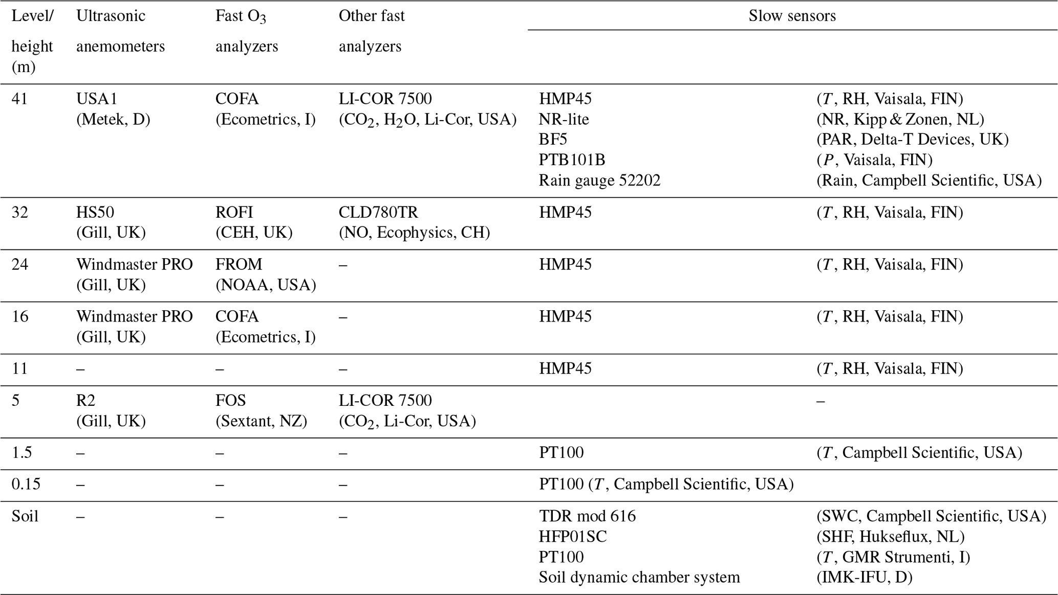
Table 1Instruments installed at each level of the tower and on the mast at 5 m a.g.l. In brackets the variable measured by each instrument and the manufacturer are indicated. (T is air temperature, RH is relative humidity, NR is net radiation, P is pressure, Rain is precipitation, SWC is soil water content, SHF is soil heat flux.) The soil dynamic chamber system is described in the methodological part.
2.4 Soil NO, NO2 and O3 flux measurements
Fluxes and concentrations of NO, NO2 and O3 at the soil–atmosphere interface were determined by use of a fully automated measuring system as described in detail elsewhere (Butterbach-Bahl et al., 1997; Gasche and Papen, 1999; Rosenkranz et al., 2006; Wu et al., 2010). Briefly, five dynamic measurement chambers and one dynamic reference chamber were installed at the site. Dimensions of the chambers were 0.5 m × 0.5 m × 0.15 m (length × width × height). In contrast to the measuring chambers, the reference chamber was sealed gastight against the soil surface using a plate made of Perspex. A 1 h resolution was chosen for flux measurements. Every chamber was closed and measured for 6 min, and before each sampling of a measuring chamber the reference chamber was sampled, resulting in a measuring cycle of 60 min. During sampling, the air from the chambers was sucked at a constant rate of 50 L min−1 and transported via PTFE tubing (inner diameter: 10 mm, length 20 m) to the analyzers. NO and NO2 concentrations were determined using a chemiluminescence detector CLD 770 AL equipped with a photolytic converter (models CLD 770AL and PLC 760, Ecophysics, CH), and O3 concentrations were determined using a UV O3 analyzer (model TE49C, Thermo Environmental Instruments, USA). Corrections for initial concentrations of NO, NO2 and O3 at the outlet of each chamber and calculation of fluxes of NO and NO2 was performed according to Butterbach-Bahl et al. (1997). Calibration of the chemiluminescence detector was performed weekly using 40 ppb NO in synthetic air produced by dilution of standard gas (4 ppm NO in N2) with synthetic air (80 % N2, 20 % O2) using a multigas calibrator (model 6100, Environics, USA). Efficiency of photolytic conversion of NO2 to NO was determined at least weekly as described in detail by Butterbach-Bahl et al. (1997).
2.5 Vertical profile of O3 and NOx concentrations and air temperature and humidity
A computer-driven system of Teflon tubes and solenoidal Teflon valves was used to characterize the vertical concentration profile of O3 and NOx above and within the canopy at six heights: 5, 8, 16, 24, 32 and 41 m. The air samples drawn through 3∕8 in. ID Teflon tubes (all of them 50 m long) from each level by a 30 L min−1 pump were sequentially sent to a UV O3 photometer (model 49C, Thermo Scientific, USA) and to a NOx chemiluminescence analyzer (model 42C, Thermo Environmental Instruments, USA) lodged in an air-conditioned container at the bottom of the tower. Both analyzers were subsampling at 2 L min−1 out of the 3∕8 ID sampling lines.
All the tubes were insulated and continuously purged. Each level was sampled for 4 min after a 1 min wait to let the analyzers stabilize and then concentration data were recorded as half-hourly averages with a customized LabVIEW program (National Instruments, USA).
The O3 gradient analyzer was calibrated against a reference photometer before and after the field campaign and no significant deviation from the first calibration was observed. The NOx analyzer was calibrated with the same procedure described above for the Ecophysics CLD780TR at the beginning of the experiment and then weekly.
Additional O3 and NOx concentrations at 0.15 m were also available from the soil chambers system previously described.
The O3 concentrations at 5, 16, 24, 32 and 41 m were also used as absolute O3 reference for the fast O3 instruments all of which change sensitivity sufficiently fast to require constant calibration against a slow-response absolute instrument.
Five temperature and relative humidity probes (model HMP45, Vaisala, Finland) were installed, at the higher tower levels (16, 24, 32 and 41 m) and, additionally, at 11 m. All these probes were connected to a data logger (CR23x, Campbell Scientific, USA), sampled once per minute and stored as half-hourly averages. Two additional temperature sensors (PT100, Campbell Scientific, USA) were available at 1.5 m and 0.15 m a.g.l. and data were collected with the same personal computer used for the control of the dynamic chamber system.
2.6 Additional meteorological and agrometeorological measurements
On the top of the tower a net radiometer NR-lite (Kipp & Zonen, NL), a BF5 sunshine sensor for total and diffuse PAR (Delta-T Devices, UK), a PTB101B barometer (Vaisala, Finland) and a rain gauge (model 52202, Campbell Scientific, USA) were mounted.
Several soil probes were installed at a distance of 20 m from the bottom of the tower: four reflectometers for soil water content (model TDR 616, Campbell Scientific, USA), four soil heat flux plates (model HFP01SC, Hukseflux, NL) and four soil temperature probes (PT100, GMR Strumenti, I). All these sensors were connected to a data logger (CR13x, Campbell Scientific, USA), sampled with a 1 min resolution and data were stored as half-hourly averages.
2.7 Measuring period
The measuring campaign began on 12 June and ended 1 month later, on 11 July 2012. From 12 to 23 June three fast O3 instruments (ROFI, FROM and one of the two COFA samplers) were all placed above the canopy at a height of 32 m in order to compare them and to characterize their performances (“intercomparison period”). The COFA installed at the top of the tower started its measurements on 12 June and was not moved to the 32 m level for the intercomparison because it was already compared with the second COFA before the campaign.
The intercomparison test allowed the agreement between the three instruments to be verified, and the average relative standard deviation was below 10 %. Considering the intrinsic variation due to the different behavior of individual coumarin targets no systematic correction was applied. The sextant analyzer, the one employed at 5 m, was calibrated after the field campaign against one of the two COFA. Also in this case, no significant deviation was observed and no corrections were applied.
On 24 June each fast O3 instrument was moved to a different level (Table S1 in the Supplement) to begin the flux profile measurements, which ended on 11 July (“Flux Profile period”). Every average diel course showed in the results section is referred to this period.
The FOS installed at 5 m was checked after the field campaign by running it in parallel with the COFA previously used at 32 m in the intercomparison period.
2.8 Data processing
The flux measurement technique adopted here was the eddy covariance method (Foken, 2008), which states that fluxes are equal to the covariance between the vertical wind component and the scalar of interest (Arya, 2001). An averaging period of 30 min was chosen for the calculation of the covariances.
2.8.1 Despiking
The data series were divided into 2 min subseries and for each of them block average and standard deviation were calculated. Spikes were identified as the instantaneous data that exceeded the average of each subseries for more than 3.5 times the standard deviation, as proposed by Vickers and Mahrt (1997). Spikes were removed from the series and the data were then gap-filled by a linear interpolation.
2.8.2 Rotations
Two axis rotations were applied to the instantaneous wind components to align u with the mean flow over the averaging period: the first rotation aligned the horizontal wind to the 30 min average u component (this rotation forces ), and the second one to rotate the xy plane in order to zero the 30 min average vertical component of the wind () (McMillen, 1988; Wilczak et al., 2001). These rotations corrected the little imperfections in the vertical alignment of the sonic anemometers and prepare data for flux calculations. Samples with a second rotation (vertical tilt) angle greater than 15∘ were discarded.
2.8.3 Linear detrending
The fluctuations of each parameter (w′, T′, O3′) were calculated as the differences of each instantaneous value from the best linear fit (minimum square) of the considered time series during each half hour (Lee at al., 2004).
2.8.4 Time-lag determination
O3 fluxes were calculated using a fixed time lag between the vertical wind time series and the O3 concentration one. For each fast instrument the time lag that maximized the cross-covariance function between the vertical component of the wind and the O3 concentrations was identified and the more frequent lag was used in the calculations for each half-hourly average flux.
2.8.5 Elimination of the kinematic fluxes below the error threshold
The error threshold was quantified for each half-hourly data series by following the methodology proposed by Langford et al. (2015). The standard deviation of the auto-correlation function was calculated for each half-hourly data chunk, with lags ranging between 30 and 60 s from the characteristic time lag of each instrument. Kinematic fluxes lower than 3 times the standard deviation (relating to the 95th percentile) were discarded.
2.8.6 Frequency loss correction
The frequency loss correction factors for the different fast O3 analyzers were calculated using the experimental transfer function approach following the methodology proposed by Aubinet et al. (2000). This method considers the normalized cospectra for sensible heat as unaffected by frequency loss or, at most, affected by frequency loss that is negligible with respect to those related to the other considered scalar (O3, NO, H2O). The transfer function is calculated for each half-hourly average as the ratio between the normalized cospectra of O3 (in our case) and the normalized cospectra of sensible heat, then fitted with a Gaussian-type function (Aubinet et al., 2001), and thus used to calculate a correction factor for each instrument. For further details, please refer to Aubinet et al. (2012).
2.8.7 Schotanus and WPL corrections
Fluxes of sensible heat (H), latent heat (LE) and trace gases were corrected for air density fluctuations. The formulation adopted for the correction of H was the one proposed by Schotanus et al. (1983) while the formulation used for LE and trace gases was the one proposed by Webb et al. (1980).
2.8.8 Calculation of fluxes in physical units
Fast O3 concentration data (acquired as voltages) and fast NO concentration data (acquired as counts per second) required additional processing to calculate quantitative fluxes in physical units. First, for all the fast O3 instruments the target zero V0 (Muller et al., 2010) – i.e., the output voltage when O3 concentration is 0 ppb – was identified for each coumarin target employed. Then the O3 fluxes were calculated by the following equation (Muller et al., 2010):
where is the covariance between the vertical wind component and the raw output voltage of the fast O3 instrument, is the half-hourly average output voltage of the instrument, V0 is the zero target (identified for the considered half hour; it represents an estimation of the voltage at zero O3 concentration) and is the O3 concentration measured by the reference O3 analyzer averaged over the same period. The data of the 2 h following each target change were excluded in order to allow the target sensitivity to stabilize after the target installation.
Similarly, NO fluxes (FNO) were calculated using the following equation:
where cps (counts per second) is the raw signal of the NO analyzer photomultiplier and the prime stands for variation around the mean, and SNO is the sensitivity of the analyzer determined by calibration against standard gases. SNO ranged from 10 000 to 12 000 cps µmol−1 m−3).
2.8.9 Ozone storage
O3 fluxes measured by eddy covariance were corrected for the O3 storage every half hour. The O3 storage is the temporal variation of the vertical O3 profile below the measuring point located at the height zm. It does not represent a true O3 removal or production process, but only a temporary accumulation of O3 in the air column below the measuring point or a temporary O3 release out of the same air column. For a nonreactive tracer, the proof of it is that the storage integrated over a whole day is null. The calculation of the O3 storage is necessary for a proper determination of the O3 deposition processes.
The correction of the O3 fluxes for the storage was made by means of the following equation (Rummel et al., 2007):
where are the O3 fluxes corrected by storage, are the measured O3 fluxes obtained with the Eq. (1), and the second term on the right represents the O3 storage term. For a reactive tracer like O3 some of the stored gas may be destroyed by reaction with NO and potentially with VOCs before being re-released to the air space above, and thus Eq. (3) must be considered an approximation. A fully resolving 1-D chemistry and exchange model would be required to quantify the effect of chemistry on the storage term more fully.
2.8.10 Stationarity check
Finally, the stationarity of each half-hourly sample was verified following the methodology of Foken and Wichura (1996) and the nonstationary data were discarded.
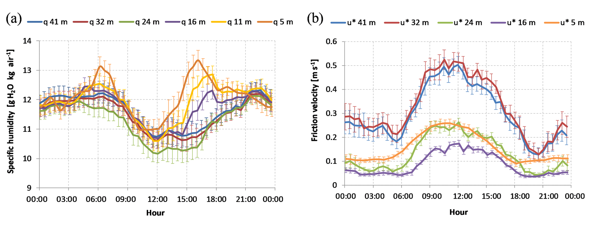
Figure 1(a) Average diel course of specific humidity (q) at the five levels; (b) average diel course of friction velocity (u*) at the five levels. Vertical bars represent the standard error of the mean.
3.1 Microclimate
Significant rainfall had cooled the air before the beginning of the field campaign so that air temperature increased significantly only during the first days and then remained stable (Fig. S1a in the Supplement). The average temperature at the top of the tower was 25.9 ∘C, while the lowest average temperature (23.1 ∘C) was recorded at 0.15 m. The maximum temperature during the whole period was 36.2 ∘C, which was observed at the top of the canopy (24 m).
On average the minimum temperature was registered during the night, at around 03:00 LT (local solar time, always the same hereafter) (Fig. S1b) for the 11 and 24 m levels and 1 h later for all the other levels, with values ranging from 19 to 21 ∘C. Two significant rainfall events occurred in the final part of the campaign, accounting for a total of 108 mm of rain, but these did not significantly affect the air temperature (Fig. S1a). In general, most of the days were sunny (only three days were partially cloudy) and humid, with nighttime peaks of relative humidity up to 80 % and diurnal minima around 40 %. Specific humidity q ranged, on average, between 10 and 13 g kg (Fig. 1a). Below-canopy levels (≤16 m) showed higher q than the above-canopy levels early in the morning, at around 06:00 LT, and from 13:00 to 21:00 LT, while the top-crown level (24 m) showed the lowest q values from 04:00 to 16:00 LT. Similar specific humidity values were registered for the above-canopy levels, with slightly higher values at 41 m.
The wind blew mostly from the E or the W directions, with about 50 % of the data in these directions (Fig. S1c), while the north and south directions accounted for 12 % of the data and the intermediate directions accounted for less than 20 % of the data. The diurnal wind intensity at 41 and 32 m was on average around 2 and 1.5 m s−1 respectively (Fig. S1d), and the wind intensity was slightly greater during the night than during daytime, with nearly 1 m s−1 more at 41 m and 0.5 m s−1 at 32 m. The three lower levels showed very low intensity, below 0.5 m s−1, with only a minor increase during the day.
The friction velocity (u*) at the two upper levels above the canopy showed a very similar behavior (Fig. 1b) but u* was slightly higher at 32 m (+6 %). Diel maxima of u* of about 0.5 m s−1 occurred between 09:00 and 13:00 LT, followed by a prompt decrease of nearly 20 % and then a gradual decrease. The minimum (0.13 m s−1) was observed around 20:00 LT, while values between 0.2 and 0.3 m s−1 were observed during the night. The in-canopy measurements of friction velocity at the lowest three levels were significantly lower than the above-canopy ones: 24 and 5 m measurements were less than 50 % of the two upper levels and 16 m measurements were around 70 % less than above-canopy levels. The diurnal maxima at noon were 0.25 m s−1 at 24 m, 0.18 m s−1 at 16 m and 0.26 m s−1 at 5 m, and during the night the friction velocity showed an almost constant trend with values around 0.1 m s−1 at 5 m and around 0.05 m s−1 for the two other levels.
3.2 Profiles of temperature, heat fluxes and atmospheric stability
In the early morning hours after sunrise, the heating of the top part of the canopy developed a thermal inversion in the forest with the ceiling at the top of the canopy (level 24 m) and the base at ground level (Fig. 2a).
Above the canopy temperature gradients were strongly superadiabatic from 04:00 to 17:00 LT; however, it should be noted that heat transfer increased significantly only when friction velocity increased.

Figure 2Diurnal evolution of vertical profile of air temperature. (a) From 0:00 to 06:00 LT; (b) from 08:00 to 18:00 LT. The green shaded area represents the vertical distribution of the leaf area density expressed as m m (= LAI∕mheight).
During the morning, the gradual heating of the canopy reached the upper canopy layer, registering its maximum value at noon. As a consequence, the inversion ceiling was lowered to the bottom part of the tree crowns (16 m). But already from 14:00 LT the air layers in the middle of the trunk space started to cool and the inversion ceiling gradually reached the top of the canopy again. By 18:00 LT the top of the canopy had cooled sufficiently for the above-canopy atmosphere to become stable and remain in this condition until 04:00 LT (Fig. 2b).
The presence of an inside canopy thermal inversion is also confirmed by the measured sensible heat fluxes (Fig. 3). Above the canopy the heat fluxes were strongly directed upwards during the day. However, the sensible heat fluxes at 32 m were about 20 % larger than those at 41 m.
In the upper part of the crown (24 m), sensible heat fluxes were less than half the above-canopy ones in the central part of the day. On the contrary, the heat fluxes at 16 and 5 m were almost always zero or negative (directed downwards). In relation to the strengthening of the thermal inversion in the afternoon, it is worth noting that the downward heat fluxes peaked at 14:00 LT at 5 m, 2 h later at 16 m and 4 h later at 24 m.
However, the forest released most of the energy as latent heat, showing a peak of about 300 W m−2 at midday and presenting very low values at nighttime.
Above the canopy, the atmosphere was nearly always unstable during the day, while below the canopy it was mostly stable, as shown in Fig. 4. At the top canopy level (24 m) the most frequent condition in the central hours of the day was strong instability because of the canopy heating due to radiation. Remarkably, stable conditions at this level strengthened from 15:00 to 19:00 LT only during the inversion.
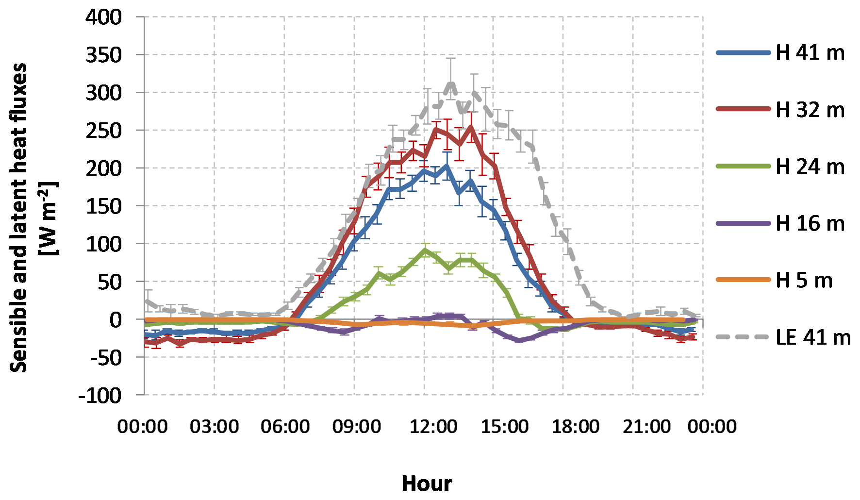
Figure 3Average diel course of sensible heat fluxes at the five levels (41, 32, 24, 16 and 5 m, thick lines) and latent heat flux at 41 m (dashed line). Vertical bars represent the standard error of the mean.
Inside the canopy (16 m), the atmosphere was mainly stable or very stable. In particular, from 14:00 to 19:00 LT the air inside canopy was almost always very stable, as also occurred in the morning from 06:00 to 08:00 LT. During the night, the atmosphere was mainly stable or very stable above the canopy, while at 24 and 16 m some nocturnal instability was observed; this instability might be due to numerical artifacts because the sensible heat fluxes were close to zero. A similar explanation can also be used for the stability class distribution at 5 m, for which some instability was observed. In any case, the stable condition was the most frequent situation observed at that level.
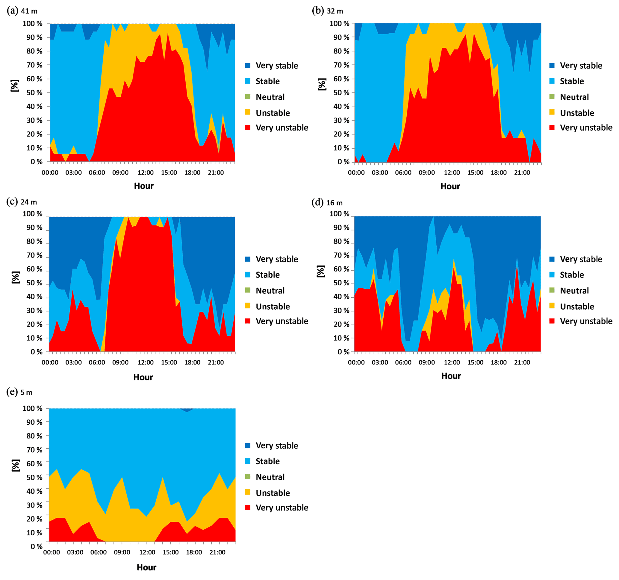
Figure 4Stability class distributions in the different hours of the day expressed as function of z∕L for the different levels: (a) 41 m, (b) 32 m, (c) 24 m, (d) 16 m and (e) 5 m. z is the measuring height while L is the Obukhov length. The stability classes were classified as follows according to Gerosa et al. (2017): very stable: ; stable: ; neutral: ; unstable: ; very unstable: .
3.3 Ozone concentrations profiles
Ozone concentrations above the canopy (41 and 32 m) showed the typical bell-shaped diurnal pattern, with a maximum around 80 ppb at 14:00 LT and a minimum around 25 ppb at 04:00 LT (Fig. 5).
The concentrations decreased slightly along the canopy height (−9 % between 32 and 5 m), while there was a significant reduction near the ground (−72 % between 32 and 0.15 m). At ground level, average O3 concentrations never exceeded 27 ppb. It is worth noting the second (relative) minimum observed at 16:00 LT at the lowest level; this minimum is in agreement with a slight reduction in the O3 concentrations observed in the upper levels inside the canopy (from 5 to 24 m). These features can be better observed considering the vertical variations in Fig. S2a and b. During the night the in-canopy gradient of O3 was negligible, but from early morning a negative gradient rapidly developed and remained almost constant (around 0.2 ppb m−1) during the daylight hours, except in the afternoon. The slope of this gradient increased in the afternoon: at 16:00 LT from 8 to 32 m (around 0.5 ppb m−1) and at 18:00 LT but only from 24 to 32 m (around 0.8 ppb m−1). Another peculiarity emerged from 13:00 to 15:30 LT, when the O3 concentration just above the canopy (32 m) was on average higher (by 2.0 to 3.8 ppb) than above (41 m); moreover, in the same period, the 24 m O3 concentration was also higher than the value measured at 41 m (assuming values from 1.2 to 2.5 ppb).
3.4 Ozone fluxes profile
Ozone fluxes were corrected for the storage in the air layers below each measuring point. The magnitude of these corrections was not negligible and they were higher in the morning and the evening (Fig. S3) when the air layers in the trunk space are refilling with and emptying of O3, respectively. Considering the whole 41 m height air column, the greatest storage correction was nearly +5 nmol m−2 s−1 in the morning, while in the evening it was about −4 nmol m−2 s−1; the integrated value over the day was null.
Ozone fluxes showed a regular behavior with almost always negative values, except for some positive peaks during the night or during the transition between night and day, in particular at the lowest levels (Fig. S4a). The largest deposition flux was observed on 25 June at 24 m with 46 nmol m−2 s−1, which is in agreement with a peak of evapotranspiration (Fig. S4b). The following 2 days, O3 fluxes and LE fluxes were nearly 50 % lower.
The good agreement between O3 fluxes and LE (water) fluxes (Fig. S4) suggested the important role of the stomatal activity in the O3 removal process because stomatal opening can increase both transpiration and O3 stomatal uptake.
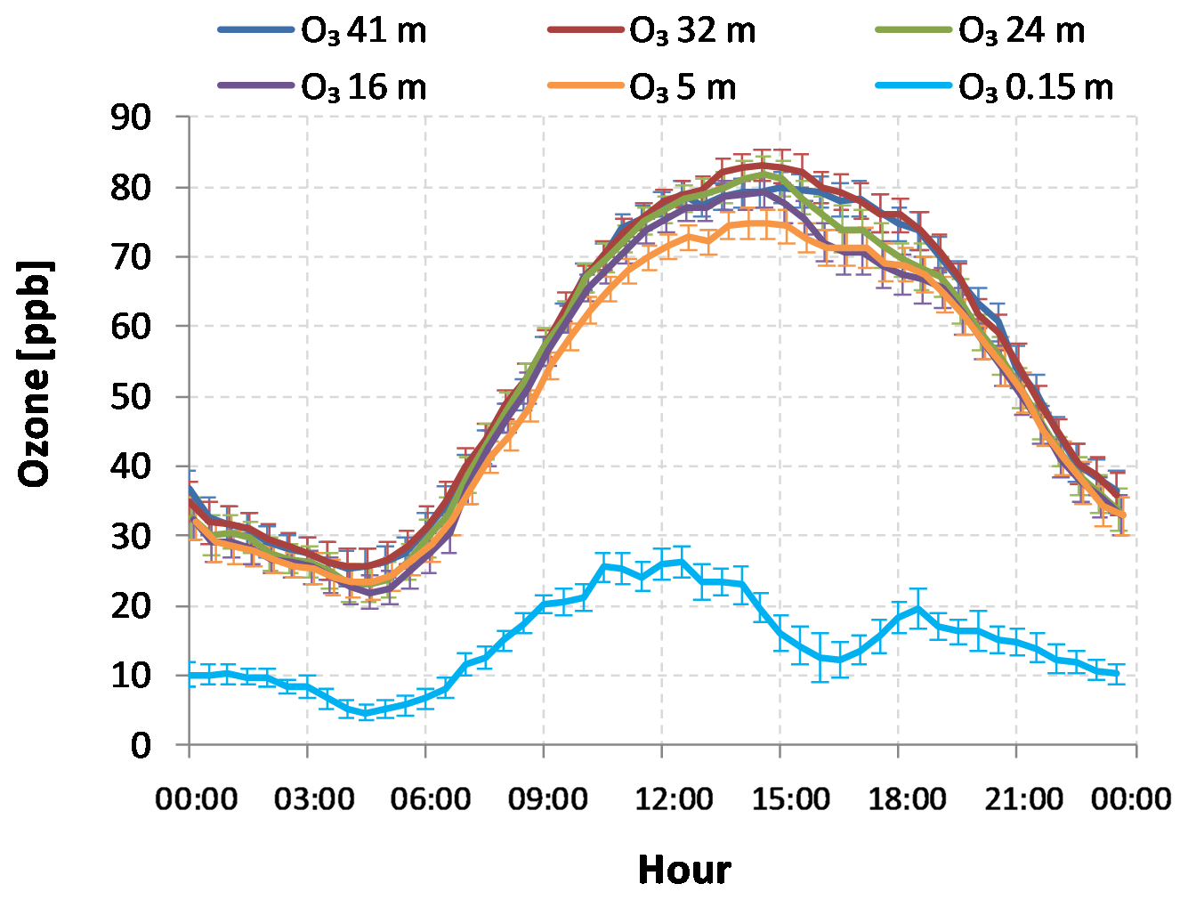
Figure 5Average diel courses of O3 concentrations at six levels (41, 32, 24, 16, 5 and 0.15 m). Vertical bars represent the standard error of the mean.
In general, O3 fluxes and LE fluxes seemed to be correlated, but there were some exceptions (e.g., on 3 and 4 July). The smallest O3 fluxes were observed on 6 July during the rainfall events, after which the O3 fluxes showed an increase (7 July) even if O3 concentrations were lower. This could be attributed to the enhancement of evapotranspiration fluxes following an increase in soil water content, even though we cannot exclude an influence of the nonstomatal processes (e.g., the increase in NO emissions from soil, Fig. 7e).
The average diel course of O3 fluxes (Fig. 6) showed the typical behavior at all levels with low nighttime values and the greatest deposition in the central hours of the day.
Ozone fluxes measured above the canopy (41 and 32 m) showed very good agreement, nearly overlapping during the day (Fig. 6). Both increased very rapidly in the morning and then stayed almost constant (between 8 and 10 nmol m−2 s−1) from 09:00 to 16:00 LT, when they started to decrease. At 24 m, fluxes were not constant in the central part of the day, and they were on average 40 % greater than the above-canopy levels, with average peaks around 15 nmol m−2 s−1 (Fig. 6). From 09:00 to 16:00 LT, air layers above the canopy including the top of the crown (from 24 m to the top of the tower) seemed decoupled from the air below: the above-canopy layers were in superadiabatic conditions with intense air mixing (Fig. 4a and b) while the below-canopy layer experienced a thermal inversion that gradually expands towards the top of the canopy and even above after 16:00 LT (Fig. 2b).
The greater fluxes at 24 m might be due to the location of these measurements, which are just in the transient region between well-mixed superadiabatic air and the below-canopy thermal inversion.
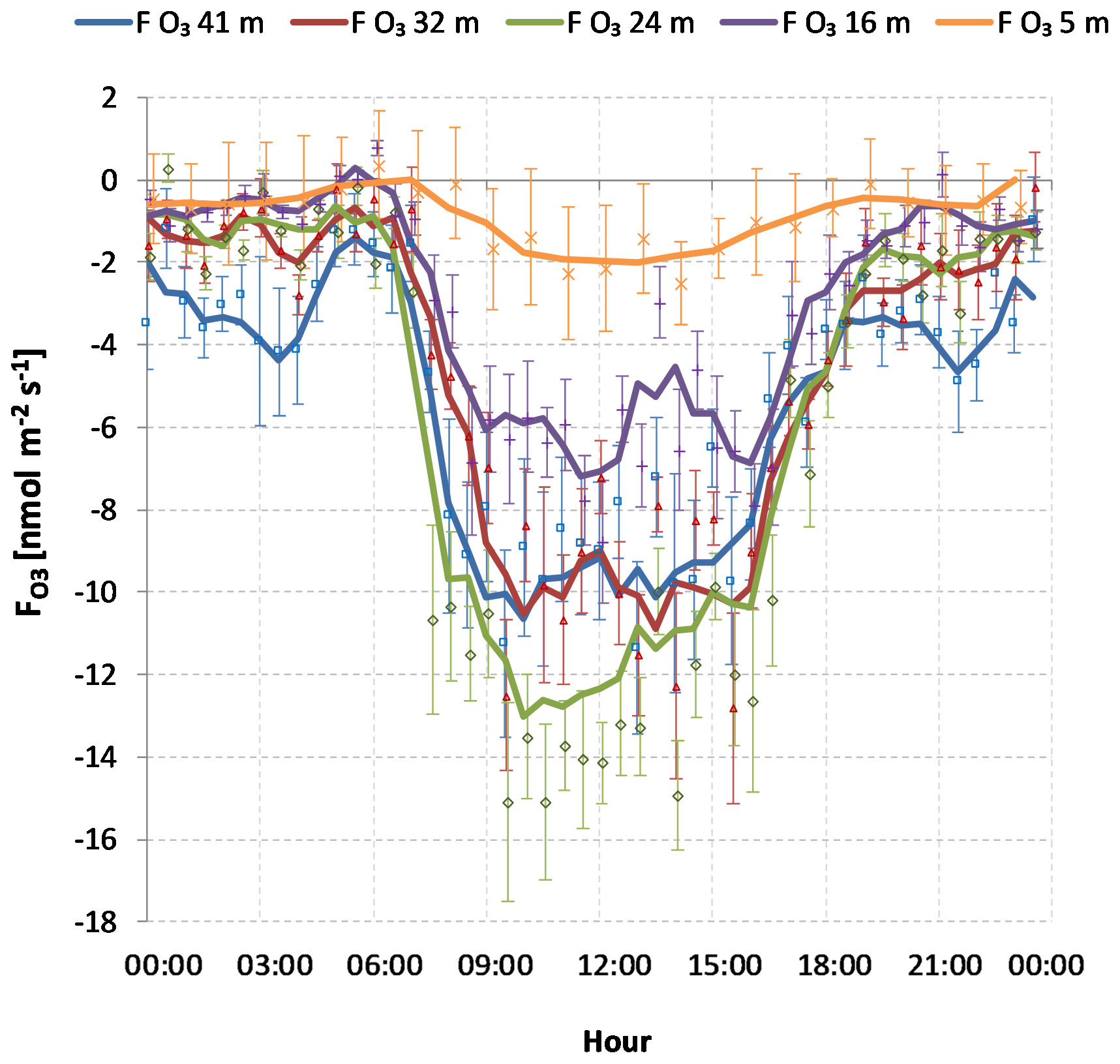
Figure 6Average diel courses of O3 fluxes at five levels (41, 32, 24, 16 and 5 m). Dots represent half-hourly averages while lines are 1.5 h running means centered on each half hour. Vertical bars represent the standard error of the mean.
3.5 NO and NO2 fluxes and concentrations
NO and NO2 concentrations along the tower profile (excluding near-ground measurements at 0.15 m) were relatively low with maximum values early in the morning of around 2 ppb for NO and around 14 ppb for NO2. Neither NO nor NO2 concentrations showed great differences along the vertical profile (Fig. 7a and b). The greatest differences between the bottom and top level were only around 1 ppb for both compounds, during the early morning hours, between 04:00 and 09:00 LT.
At soil level (0.15 m), the behavior was completely different for both compounds. NO was always greater than the above levels (from 5 to 41 m), showing two peaks (Fig. 7b): the first one around 15 ppb at 06:00 LT and the second one around 20 ppb at 17:00 LT. NO2 concentrations at soil level were relatively constant, ranging from 7 to 12 ppb; even in this case two peaks were observed: at 6:00 LT (10 ppb) and around 17:00 LT (11 ppb).
NO and NO2 fluxes at ground level were almost always monodirectional with NO emitted from soil and NO2 deposited to the ground (Fig. 7c). A strong increase in the emission rate of NO and the deposition of NO2 was observed after the precipitation events occurred between 6 and 7 July (Fig. 7d).
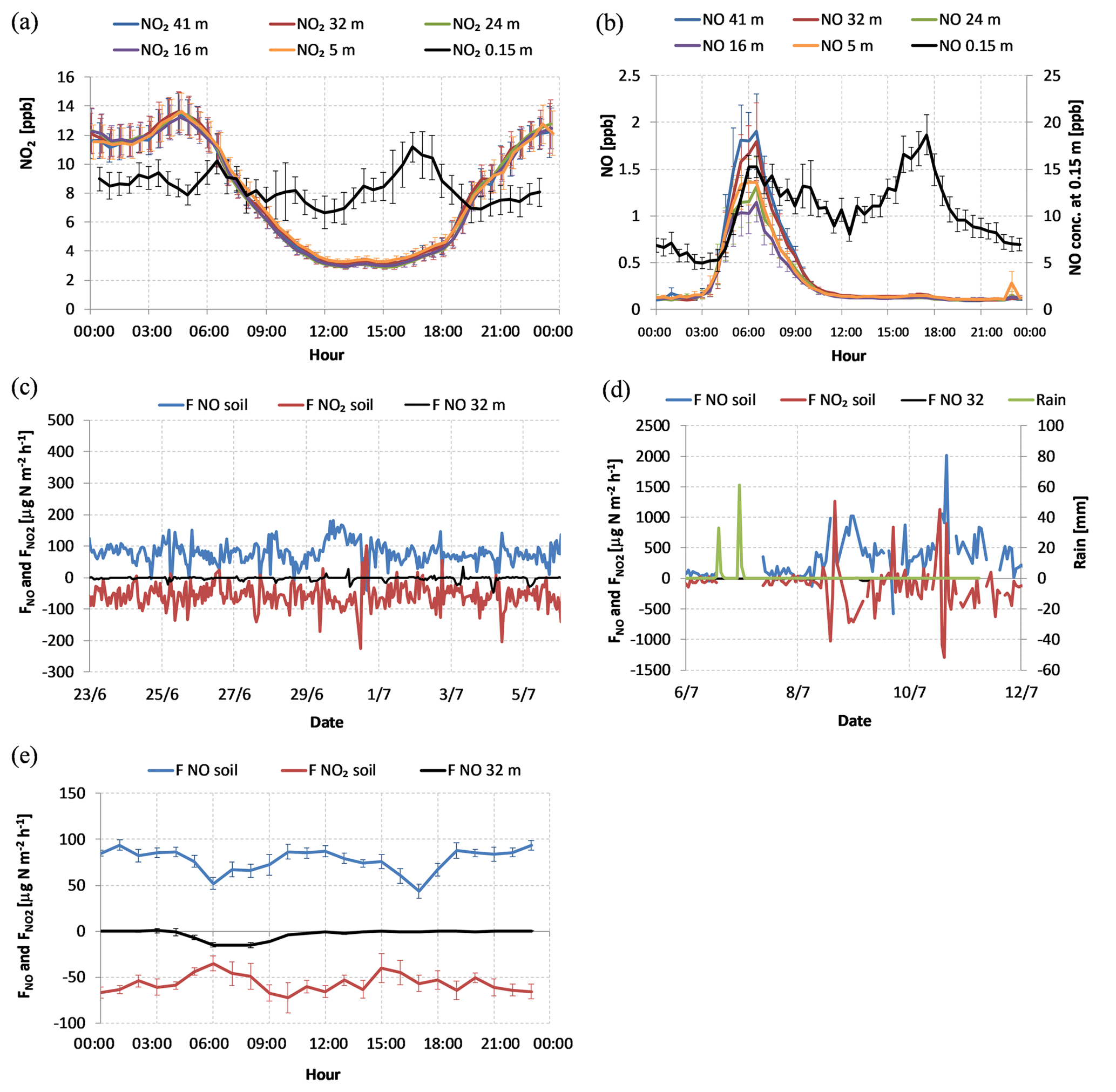
Figure 7Fluxes and concentrations of NO and NO2. (a) Average diel course of NO2 concentrations at the five levels (41, 32, 24, 16 and 5 m); (b) average diel course of NO concentrations; (c) soil NO and NO2 fluxes and NO fluxes at 32 m before rainfall events; (d) soil NO and NO2 fluxes and NO fluxes at 32 m after rainfall events (green line); (e) average diel course of soil NO and NO2 fluxes and of NO fluxes at 32 m. Please note the different scale between (c) and (d). Vertical bars in (a), (b) and (e) represent the standard error of the mean.
The average diel course of soil fluxes showed an almost constant emission of NO and two decreases: the first one around 06:00 LT and the second one at 17:00 LT. These two decreases in the observed fluxes were strictly linked to the stratification of the air above ground: an increase in the concentrations in a stratified environment led to a reduction in the concentration gradient between soil–litter and the atmosphere, thus reducing the emission fluxes. The average diel course of NO2 deposition was nearly inversely proportional to the behavior of the NO soil fluxes, with a pronounced reduction of the deposition early in the morning and a less intense one in the afternoon. In the afternoon, the nearly simultaneous minimum of soil NO fluxes and maximum of NO2 deposition (Fig. 7e) indicates a gas-phase titration with an O3 reduction due to NO (Fig. 5).
At the top of the canopy the net exchange of NO with the above atmosphere was very small, except in the morning, when the deposition peak between 06:00 and 11:00 LT reached −15 µg N m−2 s−1 (Fig. 7e). This NO deposition (Fig. 7e) is correlated to the development of a small NO gradient above the canopy (Fig. 7b) after the NO2 photolysis. The NO gradient and fluxes became negligible (Fig. 7b and e) when the NO2 concentrations reached a minimum (Fig. 7a) determined by the photolytic equilibrium of NOx.
While turbulence and heat fluxes inside tree canopies have been extensively investigated, only a few studies have attempted to partition O3 fluxes using flux measurements at different in-canopy heights (Dorsey et al., 2004; Launiainen et al., 2013).
The evaluation of flux profiles relies on the constant flux hypothesis, one of the fundamental theories of micrometeorology (Arya, 2001). In the case of the Bosco Fontana measurements, it was expected that the fluxes measured at 41 and 32 m were almost equal because both heights are above the forest canopy level, and that the deposition flux should decrease, in absolute terms, at the lower levels due to the presence of different in-canopy sinks for O3 (stomata and surfaces of the leaves, branches and stems). However, although O3 fluxes were similar at the two above-canopy heights (41 and 32 m) and within the uncertainty of the measurement, during the morning hours O3 deposition at 24 m was significantly higher than at the two upper levels (32 and 41 m). Actually, between 09:00 and 12:00 LT, O3 fluxes at 24 m were on average nearly 3 nmol m−2 s−1 higher than above the canopy (Fig. 6), while they were nearly equal between 13:00 and 18:00 LT (fluxes at 24 m were only 0.5 nmol m−2 s−1 higher).
A possible explanation of the higher O3 fluxes at 24 m could lie in the different footprints of the eddy covariance measurements coupled with the heterogeneity of the canopy (Dalponte et al., 2007; Acton et al., 2016). The footprints of the measurements at 41, 32 and 24 m all fell inside the surface of the upper forest canopy, even though the 24 m level was just at the top canopy edge. The size of the footprint areas decreased at decreasing measuring heights. However, without any source or sink of the considered scalar, the horizontal homogeneity of the ecosystem studied ensures the validity of the constant flux hypothesis and thus the measurements referred to different footprints should be the same; i.e., fluxes with larger footprints (measurements at 41 and 32 m) should be comparable to those with smaller footprints (measurements at 24 m).
Regarding the possible role of BVOC emissions on the O3 deposition fluxes, a partition exercise showed that less than 3 % of the O3 deposited to the Bosco Fontana forest was destroyed by reactions with isoprene (Eiko Nemitz, personal communication, 2013), which was the most emitted BVOC at the site (Schallahart et al., 2016). The reaction of O3 with isoprene was estimated from the methylvinylketone (MVK)/methacrolein (MACR) flux measured above the canopy by Schallahart et al. (2016) by means of a PTR-ToF spectrometer (71 atomic mass units), and by neglecting the fact that MVK/MACR can also be directly exchanged with the vegetation and produced by the competing isoprene vs. OH reaction. This result suggests a minor influence of the BVOC emissions on the enhancement of the O3 fluxes observed at the top of the canopy (24 m) in the morning. However, we cannot exclude that fast reactions between O3 and undetected highly reactive BVOCs occurred, e.g., with isoprenoids emitted at the canopy level such as the β-caryophyllene, a sesquiterpene which reacts in the gas phase in few seconds to produce both unidentified oxidized VOCs and SOA, as highlighted by Goldstein et al. (2004).
To investigate alternative reasons for the enhancement of the O3 fluxes at 24 m a spectral analysis was performed to compare the normalized cospectra of the O3 fluxes at the different levels, and the role of the NO-related O3 chemical sink was analyzed. Figure S5 shows the average normalized cospectra of the vertical component of wind and O3 for the measurements performed when the morning O3 enhancement at 24 m occurred (11:00 LT) and when the 24 m O3 fluxes were comparable with the upper ones (15:00 LT). The cospectra analysis did not provide an obvious explanation for the enhancement of the fluxes observed at 24 m in the morning. Apart from the O3 cospectra at 16 m, which had a very irregular behavior, the other three cospectra did not show any particular difference, which could explain the higher O3 fluxes at 24 m. The observed decrease in the O3 cospectra at 24 and 16 m for frequencies above 0.1 Hz is consistent with the notion that within the canopy the mean eddy size is dictated by the canopy height.
The analysis of the NO-related chemical sink revealed a possible role of the convergence of two NO fluxes at the top of the canopy (i.e., the NO deposition flux from the air above the forest and the soil NO emission flux uprising from the forest floor) on the enhancement of the O3 fluxes at 24 m. This can be argued by considering the differences between the O3 fluxes measured at 24 m and those measured at 32 m (a level where the constant flux hypothesis is confirmed). The sum of these differences from 06:00 to 12:00 LT gives a value of 59.4 µmol O3 m−2, which is almost equal to the sum of the NO converging to the top of the canopy, both from above and below in the same hours (54 µmol NO m−2).
Assuming a stoichiometric reaction between NO and O3 at the top of the canopy, the part of the O3 flux not due to this chemical sink is obtained by subtracting to the 24 m O3 fluxes value an amount of O3 equal to the NO converging at the top of the canopy during each half hour. This is shown in Fig. 8, where the measured O3 flux at 24 m is represented as a green line and the resulting part of the O3 flux at 24 m not due to the NO-related sink is reported as a dark grey dashed line, while the NO fluxes converging from above and below canopy are represented by the black and purple lines, respectively.
The good agreement during the daylight hours between the O3 fluxes at 32 m (Fig. 8, red line) and the part of the O3 flux at 24 m not due to the NO-related sink (Fig. 8, dark grey dashed line) suggests that the enhancement of the O3 fluxes observed at 24 m was related to the interactions between O3 and NO at the top canopy level. However, at night there might be an overcorrection of the O3 flux at 24 m (Fig. 8) because, in case of high atmospheric stability, the NO emitted from soil could stratify near the forest floor and react below the canopy.

Figure 8Average diel course of O3 fluxes at 32 m (red line), O3 fluxes at 24 m (green line), NO fluxes at 32 m (black line), NO fluxes at soil level (purple line) and the modified (MOD) O3 fluxes at 24 m (dashed grey line). This latter takes into account the role of the NO-related sink.
The coupling between the forest and the atmosphere above the canopy was found to have an important role on the regulation of the O3 flux enhancement at 24 m, facilitating this mechanism particularly during the morning hours when the in-canopy mixing processes were well developed. In fact, the decrease in the NO concentrations at soil level (Fig. 7b) from 06:00 to 12:00 LT suggests a relatively well-mixed forest canopy, which is better coupled with the atmosphere above. This condition also allowed O3 and NO from the above-canopy air to penetrate more easily into the canopy (see Fig. S2b and the morning peak of Fig. 7b). On the contrary, the increase in the NO concentrations at soil level (0.15 m, Fig. 7b) after midday, followed by the decrease in O3 concentrations at the same level (Fig. 5), suggests that an air stratification occurred inside the canopy in the afternoon with a decoupling from the above-canopy air, as also found by Rummel et al. (2002) and Foken (2008). The afternoon stratification was also supported by the stability classes reported in Fig. 4c and d, which denoted almost always stable or very stable atmospheric conditions both at 16 and 24 m from 15:00 to 18:00 LT. In addition, the thermal inversion layer within the canopy increased its thickness during the afternoon (Fig. 2b) rising from 16 m (around 12:00 LT) to 24 m (between 14:00 and 16:00 LT). Again, the morning coupling and the afternoon decoupling was supported by the diurnal course of the specific humidity observed below the canopy (Fig. 1a). In the morning the almost constant amount of water vapor above and below canopy (other than the 24 m level, where there was an unidentified process removing water vapor) reveals an efficient mixing of the air, while in the afternoon, the increase in the specific humidity from the three lower levels, due to soil evaporation and understorey transpiration, reveals an air stratification below the canopy and a forest decoupling from the above atmosphere.
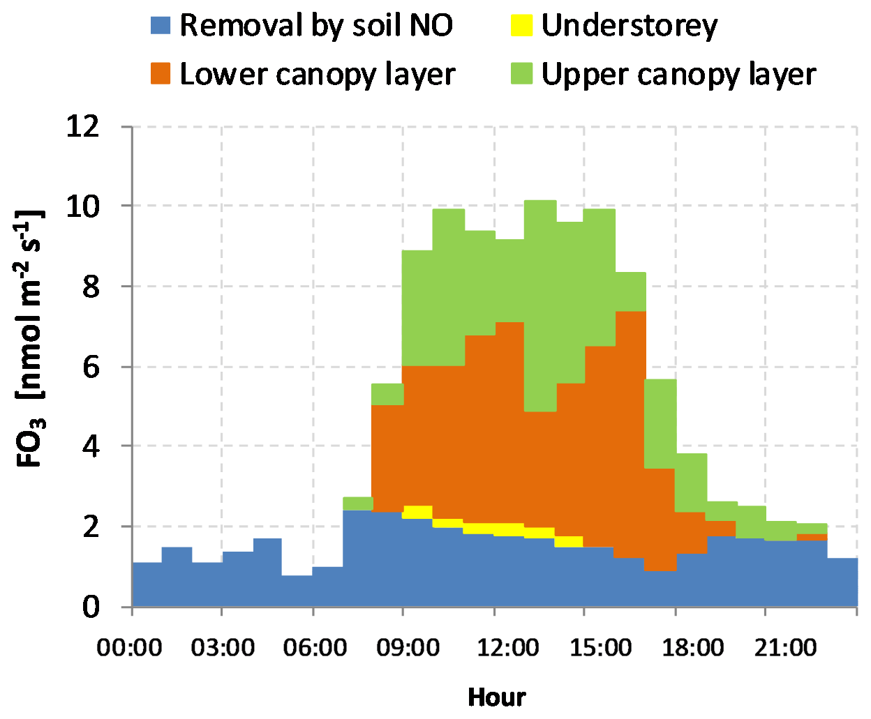
Figure 9Average diel course of the O3 removal by the different forest layers and by the NO emitted from the forest floor.
The availability of O3 flux measurements at different heights within and above the canopy allowed a partition of the O3 fluxes among the different ecosystem layers: upper and lower canopy, understorey, and soil. To do that we assumed the O3 flux measured at 32 m to be the total deposition flux, and then calculated the overall NO sink as the sum of the NO deposited from the above atmosphere and the NO emitted from the soil, considering a stoichiometric reaction between NO and O3. The O3 uptake due to the upper canopy layer was identified as the difference between the O3 fluxes measured at 32 m and those measured at 16 m (ignoring the apparently enhanced values at 24 m), while the O3 uptake due to the lower canopy layer was obtained as the difference between the O3 fluxes measured at 16 and 5 m. Finally, the deposition to the forest floor (soil and the understorey vegetation) was calculated as the difference between the O3 flux at 5 m and the NO flux emitted from the soil, namely the amount of O3, which is not removed by chemical reaction with NO.
The result of this test is shown in Fig. 9, where it can be observed that on a daily basis the upper canopy layer of the forest removed about one-third of the total deposited O3 (between 07:00 and 22:00 LT) while the lower canopy layer of the forest removed the main part of the O3 (46.5 %, between 08:00 and 22:00 LT).
The canopy removed nearly 80 % of the O3 deposited to the forest ecosystem, but it is worth noting that this amount included stomatal uptake and nonstomatal processes such as dry deposition on physical surfaces (e.g., leaves and bark) and chemical reactions in ambient air. Only a minor part of O3 was removed by the understorey vegetation or deposited to the soil (2.0 %), while an important role was played by the NO-related sink, mainly due to soil emissions, which accounted for 18.2 % of the total O3 deposition.
This latter result is in agreement with the observations of Dorsey et al. (2004) who found that in a Douglas fir plantation, between 7 % and 14 % of the O3 deposition in the daylight hours could be attributed to reactions with the NO emitted from soil, while this fraction increased up to 41 % during the night. Similarly, Pilegaard (2001) found that the NO sink accounted for 25 % of the O3 deposition in a Norway spruce forest, with an increase in this fraction up to 31 % during the night.
Nearly all of the nighttime O3 deposition at Bosco Fontana can be attributed to O3 depletion due to NO. The fact that NO reaction accounts for 100 % of the nocturnal O3 deposition would imply that other nonstomatal sinks are negligible during that time. However, it cannot be excluded that some nonstomatal deposition of O3 took place since our stirred soil flux chambers could somewhat overestimate the nocturnal soil NO emission, due to the enhanced amount of mixing in the flux chamber compared with the true forest floor during calm nights. Similarly, the analysis assumes that the only sink for NO is its reaction with O3. A small NO uptake by vegetation is possible even if unlikely, as shown by Teklemariam and Sparks (2006) and Stella et al. (2013). Overall this ecosystem did not behave as a net NO emitter because all NO produced at soil level is consumed within the canopy, but as a weak NO sink because of the small amount of NO received from the atmosphere in the first hours of the morning (Fig. 7d). This differs from the observation of Dorsey et al. (2004), who estimated that nearly 60 % of the NO emitted from the soil of a Douglas fir forest escaped the trunk space to react aloft.
Ozone flux measurements were carried out at five levels (above, inside and below the canopy) along a vertical profile of a mature broadleaf forest during the ECLAIRE joint field campaign. The data collected are particularly relevant since no measurements of O3 fluxes were previously available in the literature for an oak–hornbeam mature forest. Ozone fluxes measured at the two levels above the canopy were in good agreement and comparable to those reported for other forest types (Amthor et al., 1994; Gerosa et al., 2005; Hogg et al., 2007; Rummel et al., 2007; Finco et al., 2017). Ozone fluxes at 16 and 5 m were lower than above the canopy, while at the top canopy edge (24 m) fluxes were surprisingly higher than above in the morning hours. The main cause of this enhancement was attributed to a chemical O3 sink due to a reaction between O3 and NO, which was emitted from the soil and deposited from the atmosphere above the canopy.
The morning enhancement of the O3 fluxes at 24 m was favored by the coupling between the forest and the atmosphere, while in the afternoon the decoupling and the in-canopy stratification led to 24 m fluxes comparable to those above the canopy.
Most of the O3, nearly 80 %, was removed by the forest canopy through stomatal uptake, dry deposition on physical surfaces and ambient chemistry: in particular, the upper canopy layer removed 33.3 % of the O3 deposited and the lower canopy layer 46.3 %. Only a minor part of O3 was deposited on the soil and the understorey (2 %), while the remaining part (18.2 %) was removed by a chemical reaction with NO emitted from soil. These findings might be useful for improving the O3 risk assessment for mature forests.
The collected data will be available for the parameterization and the fine-tuning of process models aimed at correctly reproducing the in-canopy dynamics of the reactions between O3 and NOx, as these dynamics might significantly influence the biosphere–atmosphere exchange budgets of O3 and other reactive trace compounds with further implications for air quality and productivity of the forest ecosystems.
Data are freely available on request at the DATABASE REPOSITORY of the ECLAIRE fp7 Project (Owen, 2012).
The supplement related to this article is available online at: https://doi.org/10.5194/acp-18-17945-2018-supplement.
EN designed and coordinated the ECLAIRE measuring campaign at Bosco Fontana. MC, EN, AF, GG, SF and BL performed the EC and meteorological measurements at the five levels. MC performed the gas concentration measurements along the vertical profile above and within the canopy. ED-P and RG performed the soil flux measurements and their analysis. AF and GG performed the EC data processing and the full data analysis with contributions by the other coauthors. GG, AF, RM and MC wrote the paper with the contribution from all coauthors.
The authors declare that they have no conflict of interest.
The authors are grateful to the administration and the personnel of the Bosco Fontana National Reserve for their availability and continuous support, and to the European Union for having funded the project ECLAIRE under which this campaign was performed.
This publication was funded by the Catholic University of the Sacred Heart in
the framework of its programs of promotion and dissemination of the scientific research.
Edited by: Alex B. Guenther
Reviewed by: two anonymous referees
Acton, W. J. F., Schallhart, S., Langford, B., Valach, A., Rantala, P., Fares, S., Carriero, G., Tillmann, R., Tomlinson, S. J., Dragosits, U., Gianelle, D., Hewitt, C. N., and Nemitz, E.: Canopyscale flux measurements and bottom-up emission estimates of volatile organic compounds from a mixed oak and hornbeam forest in northern Italy, Atmos. Chem. Phys., 16, 7149–7170, https://doi.org/10.5194/acp-16-7149-2016, 2016.
Altimir, N., Tuovinen, J.-P., Vesala, T., Kulmala, M., and Hari, P.: Measurements of ozone removal to Scots pine shoots: calibration of a stomatal uptake model including the non-stomatal component, Atmos. Environ., 38, 2387–2398, 2004.
Altimir, N., Kolari, P., Tuovinen, J.-P., Vesala, T., Bäck, J., Suni, T., Kulmala, M., and Hari, P.: Foliage surface ozone deposition: a role for surface moisture?, Biogeosciences, 3, 209–228, https://doi.org/10.5194/bg-3-209-2006, 2006.
Amthor, J. S., Goulden, M. L., Munger, J. W., and Wofsy, S. C.: Testing a mechanistic model of forest-canopy mass and energy exchange using eddy correlation: carbon dioxide and ozone uptake by a mixed oak-maple stand, Funct. Plant Biol., 21, 623–651, 1994.
Arya, S. P.: Introduction to Micrometeorology, Academic Press, San Diego, USA, 415 pp., 2001.
Aubinet, M., Grelle, A., Ibrom, A., Rannik, U., Moncrieff, J., Foken, T., Kowalski, A. S., Martin, P. H., Berbigier, P., Bernhofer, C., Clement, R., Elbers, J., Granier, A., Grunwald, T., Morgenstern, K., Pilegaard, K., Rebmann, C., Snijders, W., Valentini, R., and Vesala, T.: Estimates of the annual net carbon and water exchange of forests: The EUROFLUX methodology, Adv. Ecol. Res., 30, 113–175, 2000.
Aubinet, M., Chermanne, B., Vandenhaute, M., Longdoz, B., Yernaux, M., and Laitat, E.: Long term carbon dioxide exchange above a mixed forest in the Belgian Ardennes, Agr. Forest Meteorol., 108, 293–315, 2001.
Aubinet, M., Vesala, T., and Papale, D. (Eds): Eddy Covariance. A practical guide to measurement and data analysis, Springer, the Netherlands, 2012.
Bauer, M. R., Hultman, N. E., Panek, J. A., and Goldstein, A. H.: Ozone deposition to a ponderosa pine plantation in the Sierra Nevada Mountains (CA): A comparison of two different climatic years, J. Geophys. Res.-Atmos., 105, 22123–22136, 2000.
Bellumè M., Maugeri M., and Mazzucchelli, E.: Due secoli di osservazioni meteorologiche a Mantova, Edizioni CUSL, Milano, Italy, 124 pp., 1998.
Büker, P., Morrissey, T., Briolat, A., Falk, R., Simpson, D., Tuovinen, J.-P., Alonso, R., Barth, S., Baumgarten, M., Grulke, N., Karlsson, P. E., King, J., Lagergren, F., Matyssek, R., Nunn, A., Ogaya, R., Peñuelas, J., Rhea, L., Schaub, M., Uddling, J., Werner, W., and Emberson, L. D.: DO3SE modelling of soil moisture to determine ozone flux to forest trees, Atmos. Chem. Phys., 12, 5537–5562, https://doi.org/10.5194/acp-12-5537-2012, 2012.
Butterbach-Bahl, K., Gasche, R., Breuer, L., and Papen, H.: Fluxes of NO and N2O from temperate forest soils: impact of forest type, N deposition and of liming on the NO and N2O emissions, Nutr. Cycl. Agroecosyst., 48, 79–90, 1997.
Campanaro, A., Hardersen, S., and Mason, F.: Piano di Gestione della Riserva Naturale e Sito Natura 2000 “Bosco della Fontana”, 4. Cierre Edizioni, Quaderni Conservazione Habitat, Verona, Italy,, 221 pp., 2007.
Cape, J. N., Hamilton, R., and Heal, M. R.: Reactive uptake of ozone at simulated leaf surfaces: implications for `non-stomatal' ozone flux, Atmos. Environ., 43, 1116–1123, 2009.
Cieslik, S.: Energy and ozone fluxes in the atmospheric surface layer observed in Southern Germany highlands, Atmos. Environ., 32, 1273–1281, 1998.
Clifton, O. E., Fiore, A. M., Munger, J. W., Malyshev, S., Horowitz, L. W., Shevliakova, E., Paulot, F., Murray, L. T., and Griffin, K. L.: Interannual variability in ozone removal by a temperate deciduous forest, Geophys. Res. Lett., 44, 542–552, 2017.
Coe, H., Gallagher, M. W., Choularton, T. W., and Dore, C.: Canopy Scale Measurements Of Stomatal And Cuticular O3 Uptake By Sitka Spruce, Atmos. Environ., 29, 1413–1423, 1995.
Dalponte, M., Giannelle, D., and Bruzzone, L.: Use of hyperspectral and LIDAR data for classification of complex forest areas, in: Canopy analysis and dynamics of a floodplain forest. Rapporti scientifici, 3, edited by: Gianelle, D., Travaglini, D., Mason, F., Minari, E., Chirici, G., and Chemini, C., Cierre Grafica Editore, Verona, 25–37, 2007.
Dorsey, J. R., Duyzer, J. H., Gallagher, M. W., Coe, H., Pilegaard, K., Weststrate, J. H., Jensen, N. O., and Walton, S.: Oxidized nitrogen and ozone interaction with forests. I: Experimental observations and analysis of exchange with Douglas fir, Q. J. Roy. Meteorol. Soc., 130, 1941–1955, 2004.
Emberson, L. D., Ashmore, M. R., Cambridge, H. M., Simpson, D., and Tuovinen, J.-P.: Modelling stomatal ozone flux across Europe, Environ. Pollut., 109, 403–413, 2000.
Ermel, M., Oswald, R., Mayer, J.-C., Moravek, A., Song, G., Beck, M., Meixner, F. X., and Trebs, I.: Preparation methods to optimize the performance of sensor discs for fast chemiluminescence ozone analyzers, Environ. Sci. Technol., 47, 1930–2936, 2013.
Fares, S., Park, J.-H., Ormeno, E., Gentner, D. R., McKay, M., Loreto, F., Karlik, J., and Goldstein, A. H.: Ozone uptake by citrus trees exposed to a range of ozone concentrations, Atmos. Environ., 44, 3404–3412, https://doi.org/10.1016/j.atmosenv.2010.06.010, 2010.
Fares, S., Weber, R., Park, J.-H., Gentner, D., Karlik, J., and Goldstein, A. H.: Ozone deposition to an orange orchard: Partitioning between stomatal and non-stomatal sinks, Environ. Pollut., 169, 258–266, https://doi.org/10.1016/j.envpol.2012.01.030, 2012.
Fares, S., Savi, F. A., Muller, J. B. A., Matteucci, G., and Paoletti, E.: Simultaneous measurements of above and below canopy ozone fluxes help partitioning ozone deposition between its various sinks in a Mediterranean Oak Forest, Agr. Forest Meteorol., 198–199, 181–191, 2014.
Finco, A., Marzuoli, R., Chiesa, M., and Gerosa, G.: Ozone risk assessment for an Alpine larch forest in two vegetative seasons with different approaches: comparison of POD1 and AOT40, Environ. Sci. Poll. Res., 24, 26238–26248, 2017.
Foken, T.: Micrometeorology, Springer-Verlag, Berlin, Heidelberg, Germany, 2008.
Foken, T. and Wichura, B.: Tools for quality assessment of surface-based flux measurements, Agr. Forest Meteorol., 78, 83–205, 1996.
Foken, T., Meixner, F. X., Falge, E., Zetzsch, C., Serafimovich, A., Bargsten, A., Behrendt, T., Biermann, T., Breuninger, C., Dix, S., Gerken, T., Hunner, M., Lehmann-Pape, L., Hens, K., Jocher, G., Kesselmeier, J., Lüers, J., Mayer, J.-C., Moravek, A., Plake, D., Riederer, M., Rütz, F., Scheibe, M., Siebicke, L., Sörgel, M., Staudt, K., Trebs, I., Tsokankunku, A., Welling, M., Wolff, V., and Zhu, Z.: Coupling processes and exchange of energy and reactive and non-reactive trace gases at a forest site – results of the EGER experiment, Atmos. Chem. Phys., 12, 1923–1950, https://doi.org/10.5194/acp-12-1923-2012, 2012.
Fontan, J., Minga, A., Lopez, A., and Druilhet, A.: Vertical ozone profiles in a pine forest, Atmos. Environ., 26, 863–869, 1992.
Fowler, D., Flechard, C., Cape, J. N., Storeton-West, R. L., and Coyle, M.: Measurements of ozone deposition to vegetation quantifying the flux, the stomatal and non-stomatal components, Water Air Soil Pollut., 130, 63–74, 2001.
Fowler, D., Pilegaard, K., Sutton, M. A., Ambus, P., Raivonen, M., Duyzer, J., Simpson, D., Fagerli, H., Sandro, F., Schjoerring, J. K., Granier, C., Neftel, A., Isaksen, I. S. A., Laj, P., Maione, M., Monks, P. S., Burkhardt, J., Daemmgen, U., Neirynck, J., Personne, E., Wichink-Kruit, R., Butterbach-Bahl, K., Flechard, C., Tuovinen, J.P., Coyle, M., Gerosa, G., Loubet, B., Altimir, N., Gruenhage, L., Ammann, C., Cieslik, S., Paoletti, E., Mikkelsen, T. N., Ro-Poulsen, H., Cellier, P., Cape, J. N., Horváth, L., Loreto, F., Niinemets, U., Palmer, P. I., Rinne, J., Misztal, P., Nemitz, E., Nilsson, D., Pryor, S., Gallagher, M. W., Vesala, T., Skiba, U., Brüggemann, N., Zechmeister-Boltenstern, S., Williams, J., O'Dowd, C., M. C. Facchini, de Leeuw, G., Flossman, A., Chaumerliac, N., and Erisman, J. W.: Atmospheric Composition Change: Ecosystems – Atmosphere interactions, Atmos. Environ., 43, 5193–5267, 2009.
Fuentes, J. D., Gillespie, T. J., Denhartog, G., and Neumann, H. H.: Ozone Deposition onto a Deciduous Forest During Dry and Wet Conditions, Agr. Forest Meteorol., 62, 1–18, 1992.
Ganzeveld, L., Lelieveld, J., Dentener, F. J., Krol, M. C., Bouwman, A. F., and Roelofs, G. J.: The influence of soil-biogenic NOx emissions on the global distribution of reactive trace gases: the role of canopy processes, J. Geophys. Res., 107, D164298, https://doi.org/10.1029/2001JD001289, 2002.
Ganzeveld, L., Ammann, C., and Loubet, B.: Modelling Atmosphere-Biosphere Exchange of Ozone and Nitrogen Oxides, in: Review and Integration of Biosphere–Atmosphere Modelling of Reactive Trace Gases and Volatile Aerosols, edited by: Massad. R.-S. and Loubet, B., Springer, Berlin, Heidelberg, Germany, 85–105, https://doi.org/10.1007/978-94-017-7285-3_3, 2015.
Gasche, R. and Papen, H.: A 3-year continuous record of nitrogen trace gas fluxes from untreated and limed soil of a N-saturated spruce and beech forest ecosystem in Germany. 2. NO and NO2 fluxes, J. Geophys. Res., 104, 18505–28520, 1999.
Gerosa, G., Vitale, M., Finco, A., Manes, F., Ballarin-Denti, A., and Cieslik, S.: Ozone uptake by an evergreen Mediterranean forest (Quercus ilex) in Italy. Part I: micrometeorological flux measurements and flux partitioning, Atmos. Environ., 39, 3255–3266, 2005.
Gerosa, G., Finco, A., Mereu, S., Vitale, M., Manes, F., and Ballarin-Denti, A.: Comparison of seasonal variations of ozone exposure and fluxes in a Mediterranean Holm oak forest between the exceptionally dry 2003 and the following year, Environ. Pollut., 157, 1737–1744, 2009a.
Gerosa, G., Finco, A., Mereu, S., Marzuoli, R., and Ballarin-Denti, A.: Interactions among vegetation and ozone, water and nitrogen fluxes in a coastal Mediterranean maquis ecosystem, Biogeosciences, 6, 1783–1798, https://doi.org/10.5194/bg-6-1783-2009, 2009b.
Gerosa, G., Fusaro, L., Monga, R., Finco, A., Fares, S., Manes, F., and Marzuoli, R.: A flux-based assessment of above and below ground biomass of Holm oak (Quercus ilex L.) seedlings after one season of exposure to high ozone concentrations, Atmos. Environ., 113, 41–49, 2015.
Gerosa, G., Marzuoli, R., Monteleone, B., Chiesa, M., and Finco, A.: Vertical ozone gradients above forests. Comparison of different calculation options with direct ozone measurements above a mature forest and consequences for ozone risk assessment, Forests, 8, 337, https://doi.org/10.3390/f8090337, 2017.
Goldstein, A. H., McKay, M., Kurpius, M. R., Schade, G. W., Lee, A., Holzinger, R., and Rasmussen, R. A.: Forest thinning experiment confirms ozone deposition to forest canopy is dominated by reaction with biogenic VOCs, Geophys. Res. Lett., 31, L22106, https://doi.org/10.1029/2004GL021259, 2004.
Güsten, H. and Heinrich, G.: On-line measurements of ozone surface fluxes: Part I. Methodology and instrumentation, Atmos. Environ., 6, 897–909, 1996.
Hogg, A., Uddling, J., Ellsworth, D., Carroll, M. A., Pressley, S., Lamb, B., and Vogel, C.: Stomatal and non-stomatal fluxes of ozone to a northern mixed hardwood forest, Tellus B, 59, 514–525, 2007.
Horvath, L., Nagy, Z., and Weidinger, T.: Estimation of dry deposition velocities of nitric oxide, sulfur dioxide, and ozone by the gradient method above short vegetation during the TRACT campaign, Atmos. Environ., 32, 1317–1322, 1998.
Jarvis, P. G.: The interpretation of the variations in leaf water potential and stomatal conductance found in canopies in the field, Philos. T. Roy. Soc. B, 273, 593–610, 1976.
Keronen, P., Reissell, A., Rannik, U., Pohja, T., Siivola, E., Hiltunen, V., Hari, P., Kulmala, M., and Vesala, T.: Ozone flux measurements over a Scots pine forest using eddy covariance 25 method: performance evaluation and comparison with flux-profile method, Boreal Environ. Res., 8, 425–444, 2003.
Kramm, G., Muller, H., Fowler, D., Hofken, K. D., Meixner, F. X., and Schaller, E.: A modified profile method for determining the vertical fluxes of NO, NO2, Ozone and HNO3 in the atmospheric surface layer, J. Atmos. Chem., 13, 265–288, 1991.
Lamaud, E., Carrara, A., Brunet, Y., Lopez, A., and Druilhet, A.: Ozone fluxes above and within a pine forest canopy in dry and wet conditions, Atmos. Environ., 36, 77–88, 2002.
Langford, B., Acton, W., Ammann, C., Valach, A., and Nemitz, E.: Eddy-covariance data with low signal-to-noise ratio: time-lag determination, uncertainties and limit of detection, Atmos. Meas. Tech., 8, 4197–4213, https://doi.org/10.5194/amt-8-4197-2015, 2015.
Launiainen, S., Katul, G. G., Gronholm, T., and Vesala, T.: Partitioning ozone fluxes between canopy and forest floor by measurements and a multi-layer model, Agr. Forest Meteorol., 173, 85–99, 2013.
Lee, X., Massman, W., and Law, B.: Handbook of Micrometeorology: A Guide for Surface Flux Measurements and Analysis, Kluwer Academic Publisher, Dordrecht, 2004.
Longo, L.: Clima, Dinamica di una foresta della Pianura Padana. Bosco della Fontana, Seconda edizione con Linee di gestione forestale, Rapporti Scientifici 1, edited by: in: Mason, F., Centro Nazionale Biodiversità Forestale Verona – Bosco della Fontana, Arcari Editore, Mantova, Italy, p 16–27, 2004.
Marzuoli, R., Bussotti, F., Calatayud, V., Calvo, E., Alonso, R., Bermejo, V., Pollastrini, M., Monga, R., and Gerosa, G.: Dose-response relationships for ozone effect on the growth of deciduous broadleaf oaks in mediterranean environment, Atmos. Environ., 190, 331–341, 2018.
Matyssek, R., Wieser, G., Calfapietra, C., de Vries, W., Dizengremel, P., Ernst, D., Jolivet, Y., Mikkelsen, T. T., Mohren, G. M. J., Le Thiec, D., Tuovinen, J. P., Weatherall, A., and Paoletti, E.: Forests under climate change and air pollution: gaps in understanding and future directions for research, Environ. Pollut., 160, 57–65, 2012.
McMillen, R. T.: An Eddy Correlation Technique with Extended Applicability to Non-Simple Terrain, Bound.-Lay. Meteorol. 43, 231–245, 1988.
Mikkelsen, T. N., Ro-Poulsen, H., Pilegaard, K., Hovmand, M. F., Jensen, N. O., Christensen, C. S., and Hummelshoej, P.: Ozone uptake by an evergreen forest canopy: temporal variation and possible mechanisms, Environ. Pollut., 109, 423–429, 2000.
Mikkelsen, T. N., Ro-Poulsen, H., Hovmand, M. F., Jensen, N. O., Pilegaard, K., and Egeløv, A. H.: Five-year measurements of ozone fluxes to a Danish Norway spruce canopy, Atmos. Environ., 38, 2361–2371, 2004.
Muller, J. B. A., Percival, C. J., Gallagher, M. W., Fowler, D., Coyle, M., and Nemitz, E.: Sources of uncertainty in eddy covariance ozone flux measurements made by dry chemiluminescence fast response analysers, Atmos. Meas. Tech., 3, 163–176, https://doi.org/10.5194/amt-3-163-2010, 2010.
Owen, S.: ECLAIRE Database, available at: http://eclairedata.ceh.ac.uk/page/login.aspx, 2012.
Padro, J.: Summary of ozone dry deposition velocity measurements and model estimates over vineyard, cotton, grass and deciduous forest in summer, Atmos. Environ., 30, 2363–2369, 1996.
Pilegaard, K.: Air–soil exchange of NO, NO2 and O3 in forests, Water Air Soil Poll., 1, 79–88, 2001.
Rannik, Ü., Altimir, N., Mammarella, I., Bäck, J., Rinne, J., Ruuskanen, T. M., Hari, P., Vesala, T., and Kulmala, M.: Ozone deposition into a boreal forest over a decade of observations: evaluating deposition partitioning and driving variables, Atmos. Chem. Phys., 12, 12165–12182, https://doi.org/10.5194/acp-12-12165-2012, 2012.
Rosenkranz, P., Brüggemann, N., Papen, H., Xu, Z., Seufert, G., and Butterbach-Bahl, K.: N2O, NO and CH4 exchange, and microbial N turnover over a Mediterranean pine forest soil, Biogeosciences, 3, 121–133, https://doi.org/10.5194/bg-3-121-2006, 2006.
Rummel, U., Ammann, C., Gut, A., Meixner, F. X., and Andreae, M. O.: Eddy covariance measurements of nitric oxide flux within an Amazonian rainforest, J. Geophys. Res.-Atmos., 107, 1–9, 2002.
Rummel, U., Ammann, C., Kirkman, G. A., Moura, M. A. L., Foken, T., Andreae, M. O., and Meixner, F. X.: Seasonal variation of ozone deposition to a tropical rain forest in southwest Amazonia, Atmos. Chem. Phys., 7, 5415–5435, https://doi.org/10.5194/acp-7-5415-2007, 2007.
Schallhart, S., Rantala, P., Nemitz, E., Taipale, D., Tillmann, R., Mentel, T. F., Loubet, B., Gerosa, G., Finco, A., Rinne, J., and Ruuskanen, T. M.: Characterization of total ecosystem-scale biogenic VOC exchange at a Mediterranean oak-hornbeam forest, Atmos. Chem. Phys., 16, 7171–7194, https://doi.org/10.5194/acp-16-7171-2016, 2016.
Schotanus, P., Nieuwstadt, F., and De Bruin, H. A. R.: Temperature measurement with a sonic anemometer and its application to heat and moisture fluxes, Bound.-Lay. Meteorol., 26, 81–93, 1983.
Stella, P., Loubet, B., Lamaud, E., Laville, P., and Cellier, P.: Ozone deposition onto bare soil: a new parameterisation, Agr. Forest Meteorol., 151, 669–681, 2011.
Stella, P., Kortner, M., Ammann, C., Foken, T., Meixner, F. X., and Trebs, I.: Measurements of nitrogen oxides and ozone fluxes by eddy covariance at a meadow: evidence for an internal leaf resistance to NO2, Biogeosciences, 10, 5997–6017, https://doi.org/10.5194/bg-10-5997-2013, 2013.
Teklemariam, T. A. and Sparks, J. P.: Leaf fluxes of NO and NO2 in four herbaceous plant species: The role of ascorbic acid, Atmos. Environ., 40, 2235–2244, 2006.
Utiyama, M., Fukuyama, T., Maruo, Y. Y., Ichino, T., Izumi, K., Hara, H., Takano, K., Suzuki, H., and Aoki, M.: Formation and deposition of ozone in a red pine forest, Water Air Soil Poll., 151, 53–70, 2004.
Vickers, D. and Mahrt, L.: Quality Control and Flux Sampling Problems for Tower and Aircraft Data, J. Atmos. Ocean. Tech., 14, 512–526, 1997.
Walton, S., Gallagher, M. W., and Duyzer, J. H: Use of a detailed model to study the exchange od NOx and O3 above and below a deciduous canopy, Atmos. Environ., 31, 2915–2931, 1997.
Webb, E. K., Pearman, G. I., and Leuning, R.: Correction of flux measurements for density effects due to heat and water vapour transfer, Q. J. Roy. Meteorol. Soc., 106, 85–100, 1980.
Wilczak, J. M., Oncley, S. P., and Sage, S. A.: Sonic anemometer tilt correction algorithms, Bound.-Lay. Meteorol., 99, 127–150, 2001.
Wittig, V. E., Ainsworth, E. A., Naidu, S. L., Karnosky, D. F., and Long, S. P.: Quantifying the impact of current and future tropospheric ozone on tree biomass, growth, physiology and biochemistry: a quantitative meta-analysis, Global Change Biol., 15, 396–424, 2009.
Wolfe, G. M., Thornton, J. A., Bouvier-Brown, N. C., Goldstein, A. H., Park, J.-H., McKay, M., Matross, D. M., Mao, J., Brune, W. H., LaFranchi, B. W., Browne, E. C., Min, K.-E., Wooldridge, P. J., Cohen, R. C., Crounse, J. D., Faloona, I. C., Gilman, J. B., Kuster, W. C., de Gouw, J. A., Huisman, A., and Keutsch, F. N.: The Chemistry of Atmosphere–Forest Exchange (CAFE) Model – Part 2: Application to BEARPEX-2007 observations, Atmos. Chem. Phys., 11, 1269–1294, https://doi.org/10.5194/acp-11-1269-2011, 2011.
Wu, X., Brüggemann, N., Gasche, R., Shen, Z., Wolf, B., and Butterbach-Bahl, K.: Environmental controls over soil-atmosphere exchange of N2O, NO, and CO2 in a temperate Norway spruce forest, Global Biogeochem. Cy., 24, GB2012, https://doi.org/10.1029/2009GB003616, 2010.
Zona, D., Gioli, B., Fares, S., De Groote, T., Pilegaard, K., Ibrom, A., and Ceulemans, T.: Environmental controls on ozone fluxes in a poplar plantation in Western Europe, Environ. Pollut., 184, 201–210, 2014.