the Creative Commons Attribution 4.0 License.
the Creative Commons Attribution 4.0 License.
Evaluating the performance of two surface layer schemes for the momentum and heat exchange processes during severe haze pollution in Jing-Jin-Ji in eastern China
Yubin Li
Changwei Liu
Tianliang Zhao
Xiaoye Zhang
Zhiqiu Gao
Tong Jiang
Huizheng Che
Meng Zhang
The turbulent flux parameterization schemes in the surface layer are crucial for air pollution modeling. There have been some deficiencies in the prediction of air pollutants by atmosphere chemical models, which is closely related to the uncertainties of the momentum and sensible heat fluxes calculated in the surface layer. The differences between two surface layer schemes (Li and MM5 schemes) were discussed, and the performances of two schemes were mainly evaluated based on the observed momentum and sensible heat fluxes during a heavy haze episode in Jing-Jin-Ji in eastern China. The results showed that the aerodynamic roughness length z0m and the thermal roughness length z0h played major roles in the flux calculation. Compared with the Li scheme, ignoring the difference between z0m and z0h in the MM5 scheme induced a great error in the calculation of the sensible heat flux (e.g., the error was 54 % at Gucheng station). Besides the roughness length, the algorithm for the surface turbulent flux as well as the roughness sublayer also resulted in certain errors in the MM5 scheme. In addition, magnitudes of z0m and z0h have significant influence on the two schemes. The large z0m and z0m∕z0h in megacities with a rough surface (e.g., Beijing) resulted in much larger differences of momentum and sensible heat fluxes between Li and MM5, compared with the small z0m and z0m∕z0h in suburban areas with a smooth surface (e.g., Gucheng). The Li scheme could better characterize the evolution of atmospheric stratification than the MM5 scheme in general, especially for the transition stage from unstable to stable atmospheric stratification, corresponding to the PM2.5 accumulation. The biases of momentum and sensible heat fluxes from Li were lower, about 38 % and 43 %, respectively, than those from MM5 during this stage. This study indicates the superiority of the Li scheme in describing regional atmospheric stratification and an improved possibility of severe haze prediction in Jing-Jin-Ji in eastern China by coupling it into atmosphere chemical models.
- Article
(7402 KB) - Full-text XML
- BibTeX
- EndNote
Adequate air quality modeling relies on the accurate simulation of meteorological conditions, especially in the planetary boundary layer (PBL) (Hu et al., 2010; Cheng et al., 2012; Xie et al., 2012). The PBL is tightly coupled with the earth's surface through turbulent exchange processes. As the bottom layer of the PBL, the surface layer (SL) reflects the surface state by calculating momentum, heat, water vapor, and other fluxes, and influences the atmospheric structure through a turbulent transport process. Many studies have illustrated the important roles of meteorological factors in the SL during air pollution formation. It has been demonstrated that weak wind speed, high relative humidity (RH), and strong temperature inversion are favorable for the concentration of haze (Zhang et al., 2014; Yang et al., 2015; Liu et al., 2017; Zhong et al., 2018). Strong stable stratification and weak turbulence are mainly responsible for many haze events. The relationship between the flux and the atmospheric profile in the atmospheric surface layer is a critical factor for air pollution diffusion, especially under stable stratification conditions (Li et al., 2017). However, there are still some uncertainties in the study of the stable boundary layer due to the poor description of surface turbulent motion. The simulation study on a severe haze in eastern China by the Weather Research and Forecasting with Chemistry (WRF-Chem) model concluded that current PBL schemes have a weak ability to distinguish between haze days under stable conditions and clean days under unstable conditions (T. Li et al., 2016). Another study (Vautard et al., 2012) of mesoscale meteorological models also pointed out there was a systematic overestimation of near-surface wind speed in the stable boundary layer which should contribute to the underestimation of surface concentrations of primary pollution. In addition, atmospheric conditions in both the PBL and upper layers are highly dependent on turbulent fluxes which are computed in the SL (Ban et al., 2010). Flux parameterization in the SL plays an important role in studies of the hydrological cycle and weather prediction (Yang et al., 2001; Li, 2014). An adequate SL scheme is crucial in providing an accurate atmospheric evolution by numerical models (Jiménez et al., 2012) and hence it may introduce significant impacts on air pollution simulation.
The bulk aerodynamic formulation based on Monin–Obukhov similarity theory (hereinafter MOST; Monin and Obukhov, 1954) is usually employed to calculate surface fluxes in numerical models. Turbulent fluxes are parameterized by wind, temperature, humidity in the lowest layer in the model, and temperature and humidity at the surface. Many international scholars verified MOST using field experiments and then proposed the universal functions, the most commonly used of which is the Businger–Dyer (BD) equation (Businger, 1966; Dyer, 1967). With the development of observation technology, the coefficients in the BD equation have been further modified (Paulson, 1970; Webb, 1970; Businger et al., 1971; Dyer, 1974; Högström, 1996). In addition to the BD equation, some other schemes have been put forward and they performed better, especially for strongly stable stratification (Holtslag and De Bruin, 1988; Beljaars and Holtslag, 1991; Cheng and Brutsaert, 2005). The schemes can be divided into two types according to the computing characteristics. One type is called an iterative algorithm (Paulson, 1970; Businger et al., 1971; Dyer, 1974; Högström, 1996; Beljaars and Holtslag, 1991), and it keeps MOST completely with less approximation so that the results can be more precise. However, many more steps are necessary for it to converge, and hence the CPU time is longer, which reduces the computational efficiency of modeling (Louis, 1979; Li et al., 2014). The other one is called a non-iterative algorithm (Louis et al., 1982; Launiainen, 1995; Wang et al., 2002; Wouters et al., 2012). There is no requirement for loop iteration in the calculation due to the approximate treatment. This algorithm is much simpler and less CPU-time-consuming, but the results are based on the loss of the calculation accuracy.
A new non-iterative scheme proposed by Li et al. (2014, 2015; Li hereinafter) speeds up effectively with a higher accuracy compared with classic iterative computation. It is remarkable that this new scheme has just been theoretically evaluated and it has never been applied in any models. Haze pollution has occurred frequently in recent years in eastern China. The concentration of PM2.5 may reach up to 1000 µg m−3 in the Beijing–Tianjin–Hebei (Jing-Jin-Ji) region in winter (Wang et al., 2014), while it is generally underestimated by current air quality models (Zhang et al., 2015; T. Li et al., 2016; Liu et al., 2017). The Li and another classic SL scheme (Zhang and Anthes, 1982; MM5 hereinafter) were compared in detail in this study. The observed momentum and sensible heat flux data covering one complete haze process at Gucheng station were used to evaluate the two schemes, focusing on the transition stage from unstable to stable atmospheric stratification, corresponding to the PM2.5 accumulation. The evaluation is in view of both local and regional scales. This study may provide the prerequisite for coupling the Li scheme into atmosphere chemical models in the future.
The definitions of momentum and sensible heat fluxes as well as the detailed algorithms of the Li and MM5 schemes are introduced in this section.
2.1 Introduction of momentum and sensible heat fluxes
The turbulent fluxes from the ground surface are defined as follows:
where τ is the momentum flux, H is the sensible heat flux, ρ is the air density, cp is the specific heat capacity at constant pressure; u∗ and θ∗ are the friction velocity and the temperature scale, respectively, and they represent the intensity of the vertical turbulent flux transport and are approximately independent of height in the SL.
Both the Li and MM5 schemes are based on bulk flux parameterization. As an important dimensionless parameter related to the stability, the bulk Richardson number RiB is defined as
where g is the acceleration of gravity, z is the reference height which is the lowest level in models, θ is the mean potential temperature at height z, θg is the surface radiometric potential temperature, and u is the mean wind speed at height z. Thus, RiB can be computed through meteorological variables from at least two levels.
2.2 The Li scheme
This new scheme employs a non-iterative algorithm to compute the surface fluxes. Its basic idea is to parameterize the stability parameter ζ directly with RiB and roughness lengths (z0m and z0h). Specifically, bulk transfer coefficients of the momentum and sensible heat fluxes (CM and CH) are expressed as
Based on MOST and considering the roughness sublayer (RSL) effect at the same time, the relationships between the bulk transfer coefficients and the profile functions corresponding to wind and potential temperature are usually expressed as
where k is the von Kármán constant, which is 0.4 in both schemes; R is the Prandtl number, which is 1.0 in the two schemes; z0m and z0h are the aerodynamic roughness length and the thermal roughness length, respectively; ψM and ψH are the integrated stability functions for momentum and sensible heat, respectively, which are also called universal functions. L is the Obukhov length (, and are the correction functions accounting for the RSL effect, and z∗ is the RSL height. It is clear to see that the calculation of the momentum and sensible heat fluxes requires CM and CH (or u∗ and θ∗), and there are three key points to consider in obtaining them:
-
z0m and z0h are two key parameters in the bulk transfer equations. Their definitions and influences will be discussed in Sect. 4.1. Note that both z0m and z0h are taken into account by the Li scheme. In other words, the Li scheme distinguishes the two principal surface parameters effectively as they generate from different mechanisms.
-
The determination of ζ is the most crucial problem in the Li scheme. In fact, this new scheme consists of two parts. The first part is proposed for atmospheric stable stratification conditions (Li et al., 2014), and the second part then extends the scheme to unstable conditions (Li et al., 2015). For stable conditions, the calculation procedure for a given group of RiB, z0m, and z0h is as follows: (1) find the region according to z0m and z0h, (2) find the section according to the region and RiB with Eq. (5) and given coefficients, and (3) calculate ζ using Eq. (6) and the given coefficients.
where Cmn and Cijk are the coefficients listed in tables in Li et al. (2014). , . m, n=0, 1, 2, and ; i, j, k=0, 1, 2, 3, and . Similarly, for unstable conditions, eight regions are divided according to the method from Li et al. (2015). For each of the regions, ζ is carried out as follows:
where Cijk is listed in Y. Li et al. (2016), and i=0, 1; j, k=0, 1, 2, 3; .
-
The universal function is also a key factor in flux calculation. The form of universal function here is adopted from Cheng and Brutsaert (2005) under stable conditions (Eq. 8a, b) and it is adopted from Paulson (1970) under unstable conditions (Eq. 9a, b):
where a=6.1, b=2.5, c=5.3, d=1.1, , .
In addition, the RSL effect is taken into account in the Li scheme. The definition and influence of the RSL will also be discussed in Sect. 4.1. De Ridder (2010) proposed the expression of and :
where υ=0.5, μM=2.59, μH=0.95, , λ=1.5; ϕM and ϕH are universal functions before integration. Here, set , :
2.3 The MM5 scheme
The MM5 scheme is a classic one which is widely applied in modeling investigations (Hu et al., 2010; Wang et al., 2015a, b; Tymvios et al., 2017). This scheme does not distinguish z0h from z0m; thus the roughness length here is expressed as z0. For unstable conditions, the function forms are given by Eq. (16a, b) following Paulson (1970), and for stable conditions, the atmospheric stratification conditions are subdivided into three cases according to Zhang and Anthes (1982) and the function forms are given by Eqs. (13), (14), and (15).
-
Strongly stable condition (RiB≥0.2):
-
Weakly stable condition ():
-
Neutral condition (RiB=0):
-
Unstable condition (RiB<0):
where , .
This scheme calculates turbulent fluxes of the momentum and sensible heat with u∗ and θ∗. In order to avoid the huge difference between the two computations, u∗ is arithmetically averaged with its previous value by Eq. (17), and a lower limit of m s−1 is imposed to prevent the heat flux from being zero under very stable conditions. According to the profile functions of wind and temperature near the ground, θ∗ is then deduced by Eq. (18).
The calculation procedure of the Li scheme is as follows: (1) determine RiB, z0m, and z0h according to the observation data; (2) calculate ζ with RiB, z0m, and z0h; and (3) calculate the momentum and sensible heat fluxes under different conditions. The MM5 scheme is summarized as follows: (1) determine the universal functions according to the values of RiB and z0, (2) calculate the u∗ and θ∗ with the meteorological variables and flux data, and (3) derive the turbulent fluxes. Compared with other non-iterative schemes including MM5, the Li scheme can be applied to the full range of roughness status and under whole conditions . In addition, there are three obvious differences between the Li and MM5 schemes: (1) Li distinguishes z0h from z0m but MM5 does not, (2) the two schemes apply different universal functions under stable conditions, and (3) Li considers the RSL effect while MM5 ignores it.
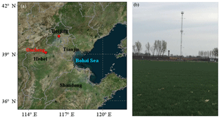
The observational fluxes used in this study were measured at Gucheng station from 1 December 2016 to 9 January 2017. Gucheng station (115.40∘ E, 39.08∘ N) is located in Gucheng County, Baoding, Hebei Province, and it is about 110 km southwest of Beijing (Fig. 1a). This station is on a farmland site where rice is grown in summer and wheat in winter. The surroundings are mainly farmland and scattered villages (Fig. 1b). At Gucheng station, the momentum and sensible heat fluxes near the surface were measured by the eddy correlation flux measurement system. The system is mainly composed of a sonic anemometer (CSAT3) and a gas analyzer (LI-7500). They are set up at a height of 4 m above the ground surface. The measured fluxes are used to evaluate the two schemes as well as estimate the roughness lengths. The measured meteorological variables including wind speed and direction, temperature, humidity, pressure, and radiation are utilized to calculate the momentum and sensible heat fluxes both in the Li and MM5 schemes. Note the observed meteorological data were from Gucheng station and national basic automatic weather stations in Jing-Jin-Ji in eastern China, respectively. Hourly surface PM2.5 mass concentration in Baoding and Beijing from the China National Environmental Monitoring Centre (http://www.cnemc.cn/, last access: 14 October 2018) was also used in this paper.
3.1 Data processing
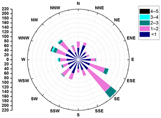
To obtain accurate flux data, quality control has been performed for the observational data, including (1) the elimination of the outliers and the data on rainy days, (2) double rotation and WPL correction (Webb et al., 1980), and (3) omission of the dataset when the wind speed is less than 0.5 m s−1. In addition, the wind field, especially the wind direction, has a great impact on the value of z0m, so it is necessary to understand the situation at Gucheng station. Figure 2 shows the distribution frequency of wind speed and wind direction at Gucheng during the observation (1 December 2016–9 January 2017). The wind speed is stable during this period and the maximum is no more than 5 m s−1, and most of them are about 1–2 m s−1. The wind direction is relatively uniform except for the southeast wind (135∘).
3.2 Determination of surface skin temperature
The surface skin temperature at Gucheng station is calculated from the radiation data by the following formula:
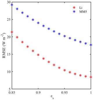
where and are the surface upward longwave radiation and longwave radiation incident on the surface, respectively; σ is the Stephen Boltzmann constant, . Tg is the surface skin temperature and εs is the surface emissivity, which is the prerequisite of Tg calculation. Many research studies estimated the value of εs and found it is always 0.9–1 (Stewart et al., 1994; Verhoef et al., 1997). According to the semi-empirical method in Yang et al. (2008), εs is estimated when the root mean square error (RMSE) is minimal. In this paper, the Li and MM5 schemes were used to estimate the εs value (as shown in Fig. 3). It is clear that the εs value corresponding to the minimum RMSE is not very sensitive to the choice of the two schemes. When εs is 1, the RMSE has a minimum value. Thus, this experiment takes 1 as the optimal value of εs.
3.3 Determination of roughness length z0m (z0h)
Using the observed momentum and sensible heat fluxes and the meteorological variables including wind speed, temperature, humidity, and pressure after quality control at Gucheng station, z0m and z0h were derived from Eq. (20a, b) following Yang et al. (2003) and Sicart et al. (2014).
During the observation period, the crops stopped growing and the height did not exceed 0.1 m, so the zero-plane displacement height was ignored and the reference height z was taken as 4 m. The observation time was too short (about 1 month) to consider the effect of seasonal variations on the roughness length. Thus, z0m and z0h were assumed to be two fixed values. Based on the variables and formulae mentioned above, the two roughness lengths at Gucheng are derived: z0m=0.0419 m and z0h=0.0042 m.
The definitions and influences of the RSL on the calculation of the turbulent flux are discussed in detail in this section. The Li and MM5 schemes are tested offline and evaluated during the haze pollution from 13 to 23 December 2016.
4.1 The influences of the RSL and roughness length on the calculation of the turbulent flux
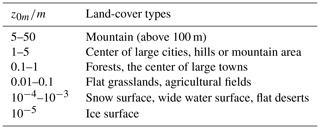
The RSL is usually defined as the region where the flow is influenced by the individual roughness elements as reflected by the spatial inhomogeneity of the mean flow (Florens et al., 2013). In the RSL, turbulence is strongly affected by individual roughness elements, and standard MOST is no longer valid (Simpson et al., 1998). Therefore, it is necessary to consider the RSL effect in the calculation of the turbulent flux, especially for rough terrain such as forest or large cities. z0m is defined as the height at which the extrapolated wind speed following the similarity theory vanishes. It is mainly determined by land-cover type and canopy height after excluding large obstructions. In models, z0m is always based on the look-up table which is related to land-cover types. In this study, z0m is simply classified based on the research of Stull (1988) and listed in Table 1. It can be seen in Table 1 that the rougher underlying surface corresponds to the larger value of z0m. z0h is the height at which the extrapolated air temperature is identical to the surface skin temperature. Some early researchers assumed that z0m was equal to z0h (Louis, 1979; Louis et al., 1982). However, the assumption is not applicable in reality because z0m and z0h have different physical meanings. Different treatments of z0m and z0h may introduce considerable changes in the surface flux calculation (Launiainen, 1995; Kot and Song, 1998; Anurose and Subrahamanyam, 2013). Many studies removed the assumption that z0m was equal to z0h and made the schemes more applicable in the situation that z0m was not equal to z0h or the ratio of z0m to z0h was much larger (Wouters et al., 2012; Li et al., 2014, 2015). Some field experiments even indicated the ratio z0m∕z0h has a diurnal variation (Sun, 1999; Yang, 2003, 2008). In this study, we make the common assumption that the ratio z0m∕z0h is a constant.
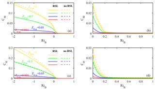
Figure 4The relationships between CM(CH) and RiB under different z0m values and treatments of the RSL. Solid lines: considering the RSL effect; dotted lines: without the RSL effect.
Considering the lowest level in mesoscale models is usually about 10 m, z=10 m is set as the reference height in this study. The range of RiB is set according to Louis et al. (1982) in the following discussion. Firstly, the study discusses the effects of different land-cover types (different z0m values) and the RSL on flux calculation. Set z0m=z0h, corresponding to four cases: z0m=1, 0.5, 0.05, and 0.001 m. These cases correspond to large cities, forests, agricultural fields, and wide water surface, respectively. Figure 4 shows the relationship between CM(CH) and RiB under different z0m values and treatments of the RSL. It can be seen that both the RSL and z0m have impacts on CM and CH. Ignoring the RSL effect can result in larger CM and CH compared with the results of the original scheme considering the RSL effect. The difference induced by the RSL effect is only evident under the rough surface. For example, the difference under z0m=1 is obviously greater than other z0m settings, and when z0m is reduced to 0.05 or less, the RSL has little effect. Furthermore, the RSL contributes more to sensible heat transfer than to momentum transfer under the same setting of z0m. The effects of different land-cover types on CM and CH are much more significant compared with the RSL. The rougher surface (corresponding to the larger z0m value) brings the larger CM (CH) under the same stability. In addition, there is a corresponding relationship between CM(CH) and stability. The value of CM(CH) drops with stability. Once RiB exceeds the critical value (generally 0.2–0.25), the transfer coefficients decline sharply but are still above 0.
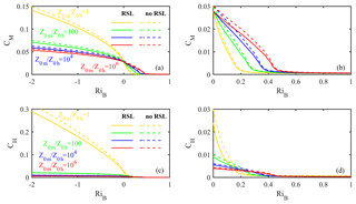
Figure 5The relationships between CM(CH) and RiB under different ratios of z0m to z0h and treatments of the RSL. Solid lines: considering the RSL effect; dotted lines: without the RSL effect.
Secondly, the effects of difference between z0m and z0h as well as the RSL on flux calculation are discussed. The relationship between z0m and z0h can be expressed as . Over the sea, z0m is comparable to z0h; over the uniform vegetation surface (e.g., grassland, farmland, woodland), kB−1 is about 2 () (Garratt and Hicks, 1973; Garratt, 1978; Garratt and Francey, 1978), which coincides with our results in Gucheng (z0m=0.0419 m, z0h=0.0042 m); over the surface with bluff roughness elements, the kB−1 value may be very large. For example, in some large cities, kB−1 is even up to 30 () (Sugawara and Narita, 2009). Therefore, the ratio z0m∕z0h varies over a wide range. Figure 5 shows the relationship between CM(CH) and RiB under different treatments of z0m∕z0h. Set z0m=1 as a large city case, z0h=1, 0.01, 10−4, and 10−6 m, and the large differences derived from the different ratios are displayed in Fig. 5. The differences induced by the RSL effect are more obvious than those in Fig. 4. The different treatments of ratio z0m∕z0h have great impacts on turbulent flux transfer, particularly for sensible heat transfer. It seems evident that when z0h is not equal to z0m (–106), the calculated CH is much smaller compared to the treatment when z0h is equal to z0m (1). In addition, CM(CH) decreases with stability, and it decreases much slower when z0h is not equal to z0m.
4.2 Comparison of momentum and sensible heat fluxes calculated by the two schemes
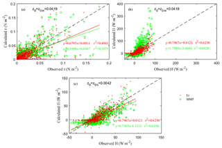
Using the obtained roughness lengths and the observations, the momentum and sensible heat fluxes were calculated by the Li and MM5 schemes. Firstly, z0m and z0h were set as 0.0419 and 0.0042, respectively, in the Li scheme, and z0 was equal to z0m in the MM5 scheme, to calculate the momentum and sensible heat fluxes, and the results are shown in Fig. 6a and b. It can be seen that compared with MM5, Li performs better with a higher regression coefficient and determination coefficient. For the momentum fluxes, the regression coefficient by Li is 0.6795 and that by MM5 is 0.5598, indicating that the error of Li is 12 % lower than that of MM5. For sensible heat fluxes, the regression coefficient by Li is 0.7967 and that by MM5 is 1.7994. The latter is much larger than 1; that is, the MM5 scheme obviously overestimates the sensible heat due to it not distinguishing z0h from z0m. Then, z0 is made equal to 0.0042 in the MM5 scheme to recalculate the sensible heat flux, and the result is shown in Fig. 6c. It can be seen that the result has a great improvement after modifying the z0 value, and the regression coefficient by MM5 is 0.7363, indicating that the error was reduced by 54 % after considering the z0h effect. The result indicates that z0h plays a critical role in both the SL scheme and the sensible heat flux (Chen and Zhang, 2009; Chen et al., 2011). However, the error of MM5 is still 6 % larger than that of Li. This illustrates that in addition to the effect of roughness length, the algorithm of the Li scheme itself is more reasonable than that of the MM5 scheme.
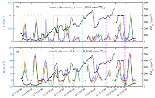
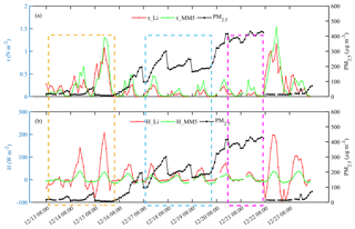
Figure 7Variations of hourly turbulent fluxes and observed PM2.5 at Gucheng station in daytime. (a) Momentum fluxes τ (blue line: observations; red line: the Li scheme; green line: the MM5 scheme) and PM2.5 concentration (black line); (b) sensible heat fluxes H (the same as τ) and PM2.5 concentration (black line). Yellow box: stage 1; blue box: stage 2; purple box: stage 3.
4.3 The specific performance of the two schemes in severe haze pollution
There were two obvious pollution processes during this observation period, and one occurred during 13 to 23 December 2016. Figure 7 shows the variations of hourly observed PM2.5 concentration as well as the momentum and sensible heat fluxes calculated by the Li and MM5 schemes at Gucheng station in this process. For research purposes, only the daytime (from 08:00 to 20:00) was taken into account. Note that in MM5, z0 was 0.0419 when calculating momentum fluxes and it was 0.0042 when calculating sensible heat fluxes. As shown in Fig. 7, the calculated results of momentum and sensible heat fluxes by the two schemes are generally consistent with the trend of the observations. Specifically, for the momentum fluxes (Fig. 7a), the results of two schemes have little difference when the values of observed momentum fluxes are large or at the peak. When the observed momentum fluxes are small, Li results are close to or less than the observations, while MM5 results are always higher than observations because of the limit of in this scheme. For the sensible heat flux (Fig. 7b), MM5 results are always lower, while Li results are closer to observations, especially when the observed values are small. Furthermore, according to the evolution of PM2.5 concentration, this haze event was then divided into three stages: the clear stage (stage 1: 13–14), the transition stage (stage 2: 16–18), and the maintenance stage (stage 3: 21–22). As shown in Fig. 7, in the clear stage (stage 1), the atmospheric stratification is unstable, PM2.5 concentration is low, and there is a strong flux transport in the SL; the corresponding observations of the momentum and sensible heat fluxes are relatively high and they vary greatly. In the transition stage (stage 2), the atmosphere is changing from being unstable to stable, corresponding to haze formation; the momentum and sensible heat fluxes gradually decrease; and the daily variation also decreases. In the maintenance stage (stage 3), the atmospheric stratification is very stable, flux transport in the SL is weak, and both the momentum and sensible heat fluxes are at a low level. It can be seen that the Li results are generally closer to the observations compared with MM5 results in all three stages.
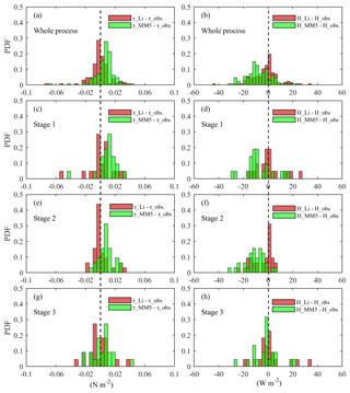
Figure 8Probability distribution functions (PDFs) of the differences between calculated fluxes (momentum fluxes: left; sensible heat fluxes: right) using two schemes (the Li scheme: red bars; the MM5 scheme: green bars) and for observations in different stages (a, b: whole process; c, d: stage 1; e, f: stage 2; g, h: stage 3).
Figure 8 shows the probability distribution functions (PDFs) of the difference between calculated fluxes (using the Li and MM5 schemes) and observations in different stages at Gucheng station. In the whole pollution process, for the momentum fluxes (Fig. 8a), the PDF from Li tends to cluster in a narrower range centered by 0, and the probability within ±0.005 N m−2 is 46.82 %, while this value from MM5 falls to 23.02 %. For the sensible heat fluxes (Fig. 8b), the PDF from Li is also more concentrated around 0 than that from MM5. The probabilities of bias from Li and MM5 within ±2.5 W m−2 are 32.54 % and 13.49 %, respectively. In stage 1, for the momentum fluxes (Fig. 8c), the probability of bias from Li within ±0.005 N m−2 is 38.09 %. The bias from MM5 is mainly larger than 0, and the probability within ±0.005 N m−2 is 14.29 %. For the sensible heat fluxes (Fig. 8d), the probability of bias from Li within ±2.5 W m−2 is 38.09 %, the same as momentum fluxes. The bias from MM5 is mainly less than 0, and the probability within ±2.5 W m−2 is 9.52 %. In stage 2, the differences between the two schemes are more obvious. The PDFs from Li are the most concentrated around 0 in all cases, while those from MM5 are similar to stage 1. Specifically, for the momentum fluxes (Fig. 8e), the probabilities of bias from Li and MM5 within ±0.005 N m−2 are 56.25 % and 25.00 %. For the sensible heat fluxes (Fig. 8f), the values within ±2.5 W m−2 are 40.62 % and 6.25 %. In stage 3, the difference between the two schemes is small. For the momentum fluxes (Fig. 8g), the probabilities of bias from Li and MM5 within ±0.005 N m−2 are 22.73 % and 27.27 %. For the sensible heat fluxes (Fig. 8h), the values from Li and MM5 within ±2.5 W m−2 are both 36.36 %.
Table 2Statistics between the Li and MM5 schemes of the calculated turbulent flux at Gucheng station.

τ: momentum flux; H: sensible heat flux; MB: mean bias; NMB: normalized mean bias; NME: normalized mean error; RMSE: root mean square error. The units of MB and RMSE are µg m−3.
Mean bias (MB), normalized mean bias (NMB), normalized mean error (NME), and root mean square error (RMSE) were calculated to test the results of the two schemes. Table 2 shows that the Li scheme generally estimates better than the MM5 scheme. In the whole haze process, the Li scheme underestimates the momentum fluxes by 3.63 % relative to the observations, while the MM5 scheme overestimates the momentum fluxes by 34.03 %. The Li and MM5 schemes underestimate the sensible heat fluxes by 15.69 % and 50.22 %, respectively. In the three stages, the Li scheme performs much better than the MM5 scheme in stage 1 and stage 2; especially in stage 2 when atmospheric stratification transforms from unstable to stable conditions, the difference between the Li and MM5 schemes is particularly significant. That is, the Li and MM5 schemes overestimate the momentum fluxes by 7.68% and 45.56 %, respectively, and they underestimate the sensible heat fluxes by 33.84 % and 76.88 %. The error of Li is much less than that of MM5. In view of the important role of atmospheric stratification in the generation and accumulation of PM2.5 in stage 2, the Li scheme is expected to show better performance in the online simulation of PM2.5 than MM5.
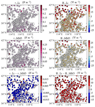
Figure 10The mean momentum and sensible heat fluxes calculated using two schemes (a, b: the Li scheme; c, d: the MM5 scheme) and their differences (Li minus MM5. e: momentum fluxes; f: sensible heat fluxes) in Jing-Jin-Ji during the haze episode (13 to 23 December 2016).
Based on the good behavior of the Li scheme in Gucheng, the same experiment was performed at Beijing station to discuss the effect of different land-cover types on flux calculation. For Beijing station, the assumption z0m=1 m, was made to represent the surface conditions of the megacity due to a lack in situ measurements of surface turbulent flux. As shown in Fig. 9, the evolution of PM2.5 concentration at Beijing station was also divided into three stages (stage 1: 13–15; stage 2: 17–19; stage 3: 20–21), like Gucheng shown in Fig. 7. Compared with Gucheng, the momentum transfer at Beijing station is obviously larger due to a great increase of the urban aerodynamic roughness length (z0m). Meanwhile, the difference between Li and MM5 is greater at Beijing station. The sensible heat transfer of the Li scheme shows a great difference between clear days and pollution days; that is, the sensible heat transfer changes acutely in stage 1, while it changes smoothly in stage 2 and stage 3. However, the result of the MM5 scheme is significantly different from the Li result due to MM5 ignoring the z0m effect, and the small number of z0h keeps the sensible heat fluxes at a low level in all three stages.
To quantify the difference between the two schemes, a relative difference is defined as a percentage:
where VLi and VMM5 are the momentum (or sensible heat) fluxes calculated by the Li and MM5 schemes, respectively. We obtained the relative differences at the two stations in the three stages through the statistics. It is clear that the largest relative difference at Gucheng station is in stage 2 and at Beijing station it is in stage 1. The differences in Beijing are always larger than those in Gucheng for each of the three stages. Specifically, the relative differences of the momentum flux in stage 1, stage 2, and stage 3 increase by 73 %, 34 %, and 27 %, respectively, and the results of the sensible heat flux are 289 %, 52 %, and 68 %, respectively.
We further estimated the surface fluxes in the whole Jing-Jin-Ji region using the two schemes. Figure 10 shows the mean momentum and sensible heat fluxes calculated by the Li and MM5 schemes and their differences in Jing-Jin-Ji during the pollution episode. The assumption (z0m=0.1 m, ) was used to represent the average conditions of the underlying surface of the Jing-Jin-Ji region. As shown in Fig. 10, the momentum fluxes calculated by Li are less than those by MM5 in most stations; the sensible heat fluxes calculated by Li are usually larger than those by MM5. The result is consistent with the experiment at Gucheng station, which further indicates the importance of considering both z0m and z0h.
Using the observed momentum and sensible heat fluxes, together with conventional meteorological data including pressure, temperature, humidity, and wind speed from 1 December 2016 to 9 January 2017, including a severe pollution episode from 13 to 23 December 2016, the differences between the Li and MM5 schemes and the specific performances of the two were discussed and evaluated in this paper. The evolution process of atmospheric stratification from unstable to stable conditions corresponding to PM2.5 accumulation was mainly discussed. The contributions of roughness lengths (z0m and z0h) as well as other factors in the SL schemes to the flux calculation for the momentum and sensible heat were also discussed in detail. The results are summarized as follows:
-
z0m and z0h have important effects on turbulent flux calculation in the SL schemes. Different values of z0m and z0h could induce great changes in the flux calculation, indicating that it is very necessary and important to distinguish z0h from z0m. Ignoring the difference between the two in the MM5 scheme led to large error in the calculation of the sensible heat flux, and this error in Gucheng was 54 %. Besides the roughness length, the algorithms in schemes are also important factors. In addition, ignoring the effect of the RSL in schemes may also result in certain bias of momentum and sensible heat fluxes in megacity regions which represent the rough underlying surface.
-
The effect of z0m∕z0h on turbulent fluxes is closely related to land-cover types (z0m). A rough land-cover type (large z0m) should be accompanied by a large value of z0m∕z0h. The differences between the two schemes for the momentum and sensible heat fluxes in Beijing were much larger than those in Gucheng. This suggests that the MM5 scheme probably induces greater error in megacities with a rough surface (e.g., Beijing) than in suburban areas with a smooth surface (e.g., Gucheng) due to the irrational algorithm of the MM5 scheme itself and the fact that the difference between z0m and z0h is ignored.
-
The Li scheme generally performed better than the MM5 scheme in the calculation of both the momentum flux and the sensible heat flux at Gucheng station. The Li scheme described atmospheric stratification, which is closely related to haze pollution, better compared with the MM5 scheme. This advantage was the most prominent in the transition stage from unstable to stable atmospheric stratification, corresponding to the PM2.5 accumulation. In this stage, the momentum flux calculated by Li was overestimated by 7.68 % and this overestimation by MM5 was up to 45.56 %; the sensible heat flux by Li was underestimated by 33.84 % while this underestimation by MM5 was as much as 76.88 %. In most of the Jing-Jin-Ji region, the momentum fluxes calculated by Li were less than those by MM5 and the sensible heat fluxes by Li were larger than those by MM5, which is consistent with Gucheng.
The offline study of the two SL schemes in this paper showed the superiority of the Li scheme for surface flux calculation corresponding to the PM2.5 evolution during haze episodes in Jing-Jin-Ji in eastern China. The study results offer a prerequisite and a possible way to improve PBL diffusion simulation and then PM2.5 prediction, which will be achieved in the follow-up work of integrating the Li scheme into atmosphere chemical models.
Data used in this paper can be provided by Yue Peng (nuist_py@163.com) upon request.
HW and YP conducted the study design. YL and CL provided the Li scheme and the flux data. CL helped with data processing. YP wrote the manuscript with the help of HW and TZ. XZ, ZG, TJ, HC, and MZ were involved in the scientific interpretation and discussion. All the authors commented on the paper.
The authors declare that they have no conflict of interest.
This article is part of the special issue “Regional transport and transformation of air pollution in eastern China”. It is not associated with a conference.
The study was supported by the National Key Project (2016YFC0203306,
2016YFC0203304), the National (Key) Basic Research and Development (973)
Program of China (2014CB441201), the National Natural Science Foundation of
China (41505004, 41675009), and Jiangsu Provincial Natural Science Fund
Project (BK20150910).
Edited by: Zhanqing Li
Reviewed by: three anonymous referees
Anurose, T. J. and Subrahamanyam, D. B.: Improvements in Sensible Heat-Flux Parametrization in the High-Resolution Regional Model (HRM) Through the Modified Treatment of the Roughness Length for Heat, Bound.-Lay. Meteorol., 147, 569–578, https://doi.org/10.1007/s10546-013-9799-9, 2013.
Ban, J., Gao, Z., and Lenschow, D. H.: Climate simulations with a new air-sea turbulent flux parameterization in the National Center for Atmospheric Research Community Atmosphere Model (CAM3), J. Geophys. Res.-Atmos., 115, D01106, https://doi.org/10.1029/2009JD012802, 2010.
Beljaars, A. C. M. and Holtslag, A. A. M.: Flux parameterization over land surfaces for atmospheric models, J. Appl. Meteor., 30, 327–341, 1991.
Businger, J. A.: Transfer of momentum and heat in the planetary boundary layer, Proc. Symp. Arctic Heat Budget and Atmospheric Circulation, RM-5233-NSF, 305–331, 1966.
Businger, J. A., Wyngaard, J. C., Izumi, Y., and Bradley, E. F.: Flux-profile relationships in the atmospheric surface layer, J. Atmos. Sci., 28, 181–189, 1971.
Chen, F. and Zhang, Y.: On the coupling strength between the land surface and the atmosphere: From viewpoint of surface exchange coefficients, Geophys. Res. Lett., 36, L10404, https://doi.org/10.1029/2009GL037980, 2009.
Chen, Y., Yang, K., He, J., Qin, J., Shi, J., Du, J., and He, Q.: Improving land surface temperature modeling for dry land of China, J. Geophys. Res.-Atmos., 116, D20104, https://doi.org/10.1029/2011JD015921, 2011.
Cheng, F. Y., Chin, S. C., and Liu, T. H.: The role of boundary layer schemes in meteorological and air quality simulations of the Taiwan area, Atmos. Environ., 54, 714–727, https://doi.org/10.1016/j.atmosenv.2012.01.029, 2012.
Cheng, Y. and Brutsaert, W.: Flux-profile relationships for wind speed and temperature in the stable atmospheric boundary layer, Bound.-Lay. Meteorol., 114, 519–538, https://doi.org/10.1007/s10546-004-1425-4, 2005.
De Ridder, K.: Bulk Transfer Relations for the Roughness Sublayer, Bound.-Lay. Meteorol., 134, 257–267, https://doi.org/10.1007/s10546-009-9450-y, 2010.
Dyer, A. J.: The turbulent transport of heat and water vapour in an unstable atmosphere, Q. J. Roy. Meteorol. Soc., 93, 501–508, https://doi.org/10.1002/qj.49709339809, 1967.
Dyer, A. J.: A review of flux-profile relationships, Bound.-Lay. Meteorol., 7, 363–372, https://doi.org/10.1007/BF00240838, 1974.
Florens, E., Eiff, O., and Moulin, F.: Defining the roughness sublayer and its turbulence statistics, Exp. Fluids, 54, 1500, https://doi.org/10.1007/s00348-013-1500-z, 2013.
Garratt, J. R.: Transfer characteristics for a heterogeneous surface of large aerodynamic roughness, Q. J. Roy. Meteorol. Soc., 104, 491–502, 1978.
Garratt, J. R. and Francey, R. J.: Bulk characteristics of heat transfer in the unstable, baroclinic atmospheric boundary layer, Bound.-Lay. Meteorol., 15, 399–421, https://doi.org/10.1007/BF00120603, 1978.
Garratt, J. R. and Hicks, B. B.: Momentum, heat and water vapour transfer to and from natural and artificial surfaces, Q. J. Roy. Meteorol. Soc., 99, 680–687, 1973.
Högström, U.: Review of some basic characteristics of the atmospheric surface layer, Bound.-Lay. Meteorol., 78, 215–246, https://doi.org/10.1007/BF00120937, 1996.
Holtslag, A. A. M. and De Bruin, H. A. R.: Applied modeling of the nighttime surface energy balance over land, J. Appl. Meteorol., 27, 689–704, 1988.
Hu, X. M., Nielsen-Gammon, J. W., and Zhang, F.: Evaluation of three planetary boundary layer schemes in the WRF model, J. Appl. Meteorol. Climatol, 49, 1831–1844, https://doi.org/10.1175/2010JAMC2432.1, 2010.
Jiménez, P. A., Dudhia, J., González-Rouco, J. F., Navarro, J., Montávez, J. P., and García-Bustamante, E.: A revised scheme for the WRF surface layer formulation, Mon. Weather Rev., 140, 898–918, https://doi.org/10.1175/MWR-D-11-00056.1, 2012.
Kot, S. C. and Song, Y.: An Improvement of the Louis Scheme for the Surface Layer in an Atmospheric Modelling System, Bound.-Lay. Meteorol., 88, 239–254, https://doi.org/10.1023/A:1001119329423, 1998.
Launiainen, J.: Derivation of the relationship between the Obukhov stability parameter and the bulk Richardson number for flux-profile studie, Bound.-Lay. Meteorol., 76, 165–179, https://doi.org/10.1007/BF00710895, 1995.
Li, T., Wang, H., Zhao, T., Xue, M., Wang, Y., Che, H., and Jiang, C.: The Impacts of Different PBL Schemes on the Simulation of PM2.5 during Severe Haze Episodes in the Jing-Jin-Ji Region and Its Surroundings in China, Adu. Meteorol., 6295878, https://doi.org/10.1155/2016/6295878, 2016.
Li, Y.: On the Surface Turbulent Fluxes Calculation in Numerical Models, University of Chinese Academy of Sciences, Beijing, 2014.
Li, Y., Gao, Z., Li, D., Wang, L., and Wang, H.: An improved non-iterative surface layer flux scheme for atmospheric stable stratification conditions, Geosci. Model Dev., 7, 515–529, https://doi.org/10.5194/gmd-7-515-2014, 2014.
Li, Y., Gao, Z., Li, D., Chen, F., Yang, Y., and Sun, L.: An Update of Non-iterative Solutions for Surface Fluxes Under Unstable Conditions, Bound.-Lay. Meteorol., 156, 501–511, https://doi.org/10.1007/s10546-015-0032-x, 2015.
Li, Y., Gao, Z., Li, D., Chen, F., Yang, Y., and Sun, L.: Erratum to: An Update of Non-iterative Solutions for Surface Fluxes Under Unstable Conditions, Bound.-Lay. Meteorol., 161, 225–228, 2016.
Li, Z., Guo, J., Ding, A., Liao, H., Liu, J., Sun, Y., Wang, T., Xue, H., Zhang, H., and Zhu, B.: Aerosol and boundary-layer interactions and impact on air quality, Natl. Sci. Rev., 4, 810–833, https://doi.org/10.1093/nsr/nwx117, 2017.
Liu, T., Gong, S., He, J., Yu, M., Wang, Q., Li, H., Liu, W., Zhang, J., Li, L., Wang, X., Li, S., Lu, Y., Du, H., Wang, Y., Zhou, C., Liu, H., and Zhao, Q.: Attributions of meteorological and emission factors to the 2015 winter severe haze pollution episodes in China's Jing-Jin-Ji area, Atmos. Chem. Phys., 17, 2971–2980, https://doi.org/10.5194/acp-17-2971-2017, 2017.
Louis, J. F.: A parametric model of vertical eddy fluxes in the atmosphere. Bound.-Lay. Meteorol., 17, 187–202, https://doi.org/10.1007/BF00117978, 1979.
Louis, J. F., Tiedtke, M., and Geleyn, J. F.: A short history of the operational PBL parameterization at ECMWF, in Workshop on Planetary Boundary Layer Parameterization, November 1981, ECMWF, Reading, UK, 59–79, 1982.
Monin, A. S. and Obukhov, A. M.: Basic laws of turbulent mixing in the surface layer of the atmosphere, Contrib. Geophys. Inst. Acad. Sci., USSR, 24, 163–187, 1954.
Paulson, C. A.: The mathematical representation of wind speed and temperature profiles in the unstable atmospheric surface layer, J. Appl. Meteorol., 9, 857–861, 1970.
Sicart, J. E., Litt, M., Helgason, W., Tahar, V. B., and Chaperon, T.: A study of the atmospheric surface layer and roughness lengths on the high-altitude tropical Zongo glacier, Bolivia, J. Geophys. Res.-Atmos., 119, 3793–3808, https://doi.org/10.1002/2013JD020615, 2014.
Simpson, I. J., Thurtell, G. W., Neumann, H. H., Den Hartog, G., and Edwards, G. C.: The Validity of Similarity Theory in the Roughness Sublayer Above Forests, Bound.-Lay. Meteorol., 87, 69–99, https://doi.org/10.1023/A:1000809902980, 1998.
Stewart, J. B., Kustas, W. P., Humes, K. S., Nichols, W. D., Moran, M. S., and De Bruin, H. A. R.: Sensible heat flux-radiometric surface temperature relationship for eight semiarid areas, J. Appl. Meteorol., 33, 1110–1117, 1994.
Stull, R. B.: An Introduction to Boundary Layer Meteorology, Kluwer Academic Publishers, London, 1988.
Sugawara, H. and Narita, K.: Roughness length for heat over an urban canopy, Theor. Appl. Climatol., 95, 291–299, https://doi.org/10.1007/s00704-008-0007-7, 2009.
Sun, J.: Diurnal Variations of Thermal Roughness Height over a Grassland, Bound.-Lay. Meteorol., 92, 407–427, https://doi.org/10.1023/A:1002071421362, 1999.
Tymvios, F., Charalambous, D., Michaelides, S., and Lelieveld, J.: Intercomparison of boundary layer parameterizations for summer conditions in the eastern Mediterranean island of Cyprus using the WRF-ARW model, Atmos. Res., 208, 45–59, https://doi.org/10.1016/j.atmosres.2017.09.011, 2017.
Vautard, R., Moran, M. D., Solazzo, E., Gilliam, R. C., Matthias, V., Bianconi, R., Chemel, C., Ferreira, J., Geyer, B., Hansen, A. B., Jericevic, A., Prank, M., Segers, A., Silver, J. D., Werhahn, J., Eolke, R., Rao, S. T., and Galmarini, S.: Evaluation of the meteorological forcing used for the Air Quality Model Evaluation International Initiative (AQMEII) air quality simulations, Atmos. Environ., 53, 15–37, https://doi.org/10.1016/j.atmosenv.2011.10.065, 2012.
Verhoef, A., De Bruin, H. A. R., and Van Den Hurk, B. J. J. M.: Some Practical Notes on the Parameter kB-1 for Sparse Vegetation., J. Appl. Meteorol., 36, 560–572, 1997.
Wang, H., Tan, S. C., Wang, Y., Jiang, C., Shi, G., Zhang, M., and Che, H. Z.: A multisource observation study of the severe prolonged regional haze episode over eastern China in January 2013, Atmos. Environ., 89, 807–815, https://doi.org/10.1016/j.atmosenv.2014.03.004, 2014.
Wang, H., Shi, G. Y., Zhang, X. Y., Gong, S. L., Tan, S. C., Chen, B., Che, H. Z., and Li, T.: Mesoscale modelling study of the interactions between aerosols and PBL meteorology during a haze episode in China Jing–Jin–Ji and its near surrounding region – Part 2: Aerosols' radiative feedback effects, Atmos. Chem. Phys., 15, 3277–3287, https://doi.org/10.5194/acp-15-3277-2015, 2015a.
Wang, H., Xue, M., Zhang, X. Y., Liu, H. L., Zhou, C. H., Tan, S. C., Che, H. Z., Chen, B., and Li, T.: Mesoscale modeling study of the interactions between aerosols and PBL meteorology during a haze episode in Jing–Jin–Ji (China) and its nearby surrounding region – Part 1: Aerosol distributions and meteorological features, Atmos. Chem. Phys., 15, 3257–3275, https://doi.org/10.5194/acp-15-3257-2015, 2015b.
Wang, S., Wang, Q., and Doyle, J.: Some improvements to Louis surface flux parameterization. Paper presented at 15th symposium on boundary layers and turbulence, American Meteorological Society, Wageningen, Netherlands, 15–19, 2002.
Webb, E. K.: Profile relationships: The log-linear range, and extension to strong stability, Q. J. Roy. Meteorol. Soc., 96, 67–90, 1970.
Webb, E. K., Pearman, G. I., and Leuning, R.: Correction of flux measurements for density effects due to heat and water vapour transfer, Q. J. Roy. Meteorol. Soc., 106, 85–100, 1980.
Wouters, H., De Ridder, K., and van Lipzig, N. P. M.: Comprehensive Parametrization of Surface-Layer Transfer Coefficients for Use in Atmospheric Numerical Models, Bound.-Lay. Meteorol, 145, 539–550, https://doi.org/10.1007/s10546-012-9744-3, 2012.
Xie, B., Fung, J. C. H., Chan, A., and Lau, A.: Evaluation of nonlocal and local planetary boundary layer schemes in the WRF model, J. Geophys. Res.-Atmos., 117, 48–50, https://doi.org/10.1029/2011JD017080, 2012.
Yang, K., Tamai, N., and Koike, T.: Analytical Solution of Surface Layer Similarity Equations, J. Appl. Meteorol., 40, 1647–1653, 2001.
Yang, K., Koike, T., and Yang, D.: Surface Flux Parameterization in the Tibetan Plateau, Bound.-Lay. Meteorol., 106, 245–262, https://doi.org/10.1023/A:1021152407334, 2003.
Yang, K., Koike, T., Ishikawa, H., Kim, J., Li, X., Liu, H., Liu, S., Ma, Y., and Wang, J.: Turbulent Flux Transfer over Bare-Soil Surfaces: Characteristics and Parameterization, J. Appl. Meteorol. Clim., 47, 276–290, https://doi.org/10.1175/2007jamc1547.1, 2008.
Yang, Y., Liu, X., Qu, Y., Wang, J., An, J., Zhang, Y., and Zhang, F.: Formation mechanism of continuous extreme haze episodes in the megacity Beijing, China, in January 2013, Atmos. Res., 155, 192–203, https://doi.org/10.1016/j.atmosres.2014.11.023, 2015.
Zhang, B., Wang, Y., and Hao, J.: Simulating aerosol–radiation–cloud feedbacks on meteorology and air quality over eastern China under severe haze conditionsin winter, Atmos. Chem. Phys., 15, 2387–2404, https://doi.org/10.5194/acp-15-2387-2015, 2015.
Zhang, D. and Anthes, R. A.: A high-resolution model of the planetary boundary layer—Sensitivity tests and comparisons with SESAME-79 data, J. Appl. Meteorol., 21, 1594–1609, 1982.
Zhang, R., Li, Q., and Zhang, R.: Meteorological conditions for the persistent severe fog and haze event over eastern China in January 2013, Sci. China Earth Sci., 57, 26–35, https://doi.org/10.1007/s11430-013-4774-3, 2014.
Zhong, J., Zhang, X., Dong, Y., Wang, Y., Liu, C., Wang, J., Zhang, Y., and Che, H.: Feedback effects of boundary-layer meteorological factors on cumulative explosive growth of PM2.5 during winter heavy pollution episodes in Beijing from 2013 to 2016, Atmos. Chem. Phys., 18, 247–258, https://doi.org/10.5194/acp-18-247-2018, 2018.


