Attributing differences in the fate of lateral boundary ozone in AQMEII3 models to physical process representations

Increasing emphasis has been placed on characterizing the contributions and the uncertainties of ozone imported from outside the US. In chemical transport models (CTMs), the ozone transported through lateral boundaries (referred to as LB ozone hereafter) undergoes a series of physical and chemical processes in CTMs, which are important sources of the uncertainty in estimating the impact of LB ozone on ozone levels at the surface. By implementing inert tracers for LB ozone, the study seeks to better understand how differing representations of physical processes in regional CTMs may lead to differences in the simulated LB ozone that eventually reaches the surface across the US. For all the simulations in this study (including WRF∕CMAQ, WRF∕CAMx, COSMO-CLM∕CMAQ, and WRF∕DEHM), three chemically inert tracers that generally represent the altitude ranges of the planetary boundary layer (BC1), free troposphere (BC2), and upper troposphere–lower stratosphere (BC3) are tracked to assess the simulated impact of LB specification.

Comparing WRF∕CAMx with WRF∕CMAQ, their differences in vertical grid structure explain 10 %–60 % of their seasonally averaged differences in inert tracers at the surface. Vertical turbulent mixing is the primary contributor to the remaining differences in inert tracers across the US in all seasons. Stronger vertical mixing in WRF∕CAMx brings more BC2 downward, leading to higher BCT ($\text{BCT}=\text{BC1}+\text{BC2}+\text{BC3}$) and BC2∕BCT at the surface in WRF∕CAMx. Meanwhile, the differences in inert tracers due to vertical mixing are partially counteracted by their difference in sub-grid cloud mixing over the southeastern US and the Gulf Coast region during summer. The process of dry deposition adds extra gradients to the spatial distribution of the differences in DM8A BCT by 5–10 ppb during winter and summer.

COSMO-CLM∕CMAQ and WRF∕CMAQ show similar performance in inert tracers both at the surface and aloft through most seasons, which suggests similarity between the two models at process level. The largest difference is found in summer. Sub-grid cloud mixing plays a primary role in their differences in inert tracers over the southeastern US and the oceans in summer. Our analysis of the vertical profiles of inert tracers also suggests that the model differences in dry deposition over certain regions are offset by the model differences in vertical turbulent mixing, leading to small differences in inert tracers at the surface in these regions.

1 Introduction

Studies based on chemical transport models (CTMs) have shown that air quality in the US can be considerably influenced by pollutants beyond the US boundaries, such as through intercontinental transport and through stratosphere-to-troposphere exchange (Zhang et al., 2011; Lin et al., 2012; Nopmongcol et al., 2016; Langford et al., 2017; Lin et al., 2017; Hogrefe et al., 2018). Similar findings have also been reported based on routine observations and field campaign measurements (e.g., Cooper et al., 2012; Gratz et al., 2015; Langford et al., 2015), especially at rural and elevated locations in the western US. Recent revisions to the National Ambient Air Quality Standards (NAAQS) further lowered both the primary (health-based) and secondary (welfare-based) standards for ground-based ozone (Federal Register, 2015). Therefore, increasing emphasis has been placed on the need to characterize the contributions and the uncertainties of ozone imported from outside the US.

The contribution of ozone from outside the US to the surface ozone within the US has been estimated by several studies with different approaches, including source sensitivity approaches (such as the “brute force” method; e.g., Dolwick et al., 2015), the path-integral method (Dunker et al., 2017), and tagged species approaches such as the integrated source apportionment method (ISAM) for CMAQ (Kwok et al., 2015), ozone source apportionment technology (OSAT) for CAMx (Ramboll, 2018), and chemically reactive tracers (Baker et al., 2015; Nopmongcol et al., 2017).

The simulated ozone levels by regional CTMs can be influenced by uncertainties in the specification of lateral boundary (LB) conditions. For example, in phase 3 of Air Quality Model Evaluation International Initiative (AQMEII3), Hogrefe et al. (2018) analyzed the impact of LB ozone derived from four global or hemispheric CTMs on the ozone predictions over the US using CMAQ and found significantly varying impacts of LB conditions on predicted surface ozone levels. Furthermore, LB ozone undergoes a series of physical and chemical processes in CTMs, which may be represented differently due to different model configurations and parameterizations chosen by the models (Russell and Dennis, 2000). Limited efforts, however, have been devoted to elucidating the reasons at the process level for the noted similarities and differences among the model predictions in surface ozone and the impact of LB ozone, though studies have suggested the important role that the processes in CTMs play in explaining the model differences. For example, also in AQMEII3, Solazzo et al. (2017) compared the model errors in surface ozone predictions over the US and Europe from several regional CTMs and showed that errors across a series of timescales could be attributed to different chemical and physical processes in the CTMs.

Understanding how the differences in model predictions can be attributed to scientific processes in CTMs is important for several reasons. First, comparison in fundamental processes can help to mitigate the reducible error in air quality models, which can be achieved through scientific improvements in the representations of the physical and chemical processes in CTMs so that model prediction from a single CTM can be improved (e.g., Zhang et al., 2012). Second, identifying the major process(es) contributing to the variability across models can help to guide research directions to reduce model uncertainty and error. Last, a better understanding of the model similarities and differences at the process level could improve multi-model ensembles by increasing the independence of ensemble members.

This study therefore focuses on examining the impact of physical treatments in CTMs on LB ozone and aims at a better understanding of how different representations of physical processes in CTMs may lead to the differences in the LB ozone that eventually reaches the surface across the US. To keep track of the LB ozone, chemically inert tracers for LB ozone have been implemented in all participating models in this study; the chemical loss of LB ozone is excluded. The important thing to clarify is that it is necessary to include the chemical loss of LB ozone when quantitatively estimating the impact of LB ozone, as shown in the comparison between inert and reactive LB ozone tracers by Baker et al. (2015). This study, instead of providing such a quantitative estimate, aims at understanding the model variability that originates from the physical treatments in CTMs and its impact on the LB ozone reaching the surface. The implementation of chemically inert tracers enables us to completely focus on the impact of physical treatments in CTMs. Otherwise, it would be very difficult to disentangle the impact of chemical processes from the impact of physical processes if chemically reactive tracers for LB ozone are employed, as chemical and physical processes are intricately coupled in CTMs.

This paper is organized as follows. Section 2 describes the model configurations and how the chemically inert tracers are implemented. In Sect. 3, the seasonal impact of physical treatment in CTMs on inert tracers at the surface is examined by comparing WRF∕CMAQ to several sensitivity simulations. Then WRF∕CMAQ is used as a base case and the differences in inert tracers between WRF∕CMAQ and three other models are investigated and discussed with respect to the physical processes in which inert tracers are involved. Finally, the findings are summarized in Sect. 4.

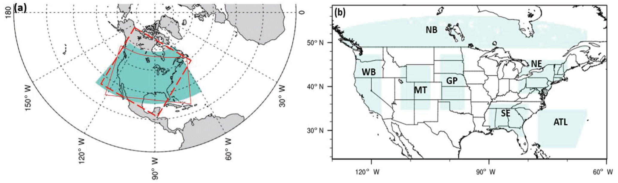
Figure 1 (a) Simulation domain for WRF∕CMAQ and WRF∕CAMx (red solid line), the simulation domain for WRF∕DEHM (red dashed line), and the analysis domain in this study (shaded area in green). The simulation domain of COSMO-CLM∕CMAQ is the same size as WRF∕CMAQ but shifts westward by 48 km. (b) The subregions in the analysis domain.

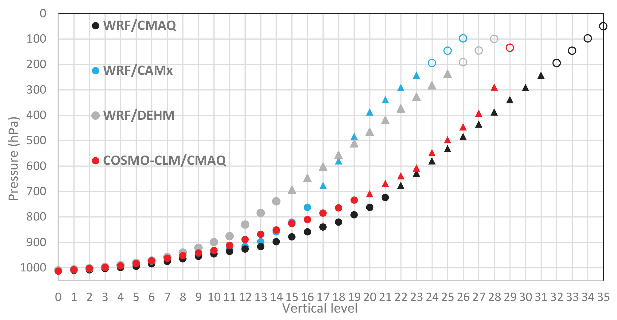
Figure 2 Vertical grid structures for the chemical transport models used in the four simulations, with filled circles for the vertical levels for BC1, filled triangles for BC2, and open circles for BC3.

2 Methods

2.1 Model description

This study, performed as part of AQMEII3, investigates simulations conducted by four research groups from the US and Europe using state-of-the-art regional CTMs. The four simulations are named using the combination of the regional CTMs and the models used to generate their meteorological inputs: WRF∕CMAQ, WRF∕CAMx, COSMO-CLM∕CMAQ, and WRF∕DEHM. A description of the model features and emissions can be found in the technical note by Galmarini et al. (2017). The simulation period is the entire year of 2010, which was determined by AQMEII3 based on the availability of emission and observation data. The chemical boundary conditions for all simulations were derived from the Composition Integrated Forecasting System (C-IFS) global modeling system (Flemming et al., 2015) by the European Centre for Medium-Range Weather Forecasts (ECMWF). The LB ozone derived from C-IFS has been evaluated against observations (Hogrefe et al., 2018). WRF∕CMAQ and WRF∕CAMx share the same modeling domain (Fig. 1a). The size of the modeling domain for COSMO-CLM∕CMAQ is like that for WRF∕CMAQ, but was shifted westward by 48 km. WRF∕DEHM, however, has a very different domain coverage than other models (Fig. 1a). Therefore, the results of inert tracers for LB ozone are directly comparable among WRF∕CMAQ, WRF∕CAMx, and COSMO-CLM∕CMAQ, but not WRF∕DEHM.

2.2 Chemically inert tracers

For each simulation, three chemically inert tracers were added specifically at the lateral boundaries to track ozone at different altitudes from outside the modeling domain. The three tracers, representing LB ozone from the planetary boundary layer (PBL), the free troposphere, and the upper troposphere–lower stratosphere, respectively, are defined as follows: BC1 for vertical layers below 750 hPa (∼2.5 km); BC2 for layers between 750 hPa (∼2.5 km) and 250 hPa (∼10 km); and BC3 for layers above 250 hPa. Initial conditions for all tracers were set to zero and a 10-day spin-up period was used in the simulations. The lateral boundary conditions (LBCs) of the tracers were set to be the same values as the LBCs of ozone at the corresponding vertical layers, with zero values assigned in other layers. For example, for WRF∕CMAQ, BC1 is the LB ozone from layer 1 to 21, BC2 from layer 22 to 31, and BC3 from layer 32 to 35 (Fig. 2). Therefore, these tracers can provide information on the altitude ranges from which the LB ozone reaching the surface originates. Due to the different vertical grid structure used by each model, differences occur in the attributions of LB ozone to inert tracers across models. For example, Fig. 2 shows the typical pressure at each vertical level for the four models. In WRF∕CMAQ, BC2 starts from layer 22, with the pressure at the bottom of the layer about 725 hPa, while in WRF∕CAMx, BC2 starts from layer 17, with the pressure at the bottom of the layer about 755 hPa. Such differences may result in differences in the relative contributions of BC1 and BC2 to the total inert tracer at the surface, but are not expected to significantly change the total amount of BC1 and BC2 reaching the surface, which is also confirmed later in Sect. 3. BC3 starts from very similar pressure levels for WRF∕CMAQ, WRF∕CAMx, and WRF∕DEHM, but is different for COSMO-CLM∕CMAQ due to its very coarse vertical resolution in the upper troposphere–lower stratosphere. The impact of such differences on inert tracers at the surface is also found to be small in general as the seasonal averaged contribution of BC3 at the surface is usually very small (less than 1.5 ppb) relative to BC1 and BC2 across the US except for summer.

Table 1 Model description of the four simulations involved in the study.

Table 2 Description of the sensitivity simulations.

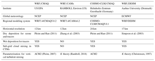
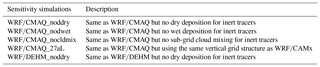
The tracers undergo the same physical processes as ozone, including 3-D advective transport, vertical turbulent mixing, sub-grid cloud mixing (if represented in CTMs), scavenging, and deposition. In all models, the deposition velocity of tracers was set to be the same as that of ozone. The physical processes that the inert tracers undergo in each model have been summarized in Table 1. To better distinguish the impact of each physical processes, a series of sensitivity simulations has been conducted for WRF∕CMAQ, including WRF∕CMAQ_noddry, WRF∕CMAQ_nodwet, and WRF∕CMAQ_nocldmix (as described in Table 2). Ideally, the sensitivity simulations conducted for WRF∕CMAQ are also desired for the other three models. However, since these sensitivity simulations were not part of the original design for AQMEII3 and entail additional nontrivial resource commitments from each participating organization, most sensitivity simulations are not available except for WRF∕DEHM_noddry (Table 2). In addition, the vertical resolution, especially in the free troposphere, has been shown to be important for air quality models (e.g., Mathur et al., 2017; Eastham and Jacob, 2017). To investigate the impact of this physical treatment on LB ozone, a sensitivity simulation WRF∕CMAQ_27aL was conducted. This simulation is the same as WRF∕CMAQ except that it uses the same vertical grid structure as WRF∕CAMx, as WRF∕CAMx has the coarsest vertical resolution in the free troposphere among the four models.

2.3 Data for analysis

Due to the different modeling domain and horizontal resolution across the models, the participating groups followed the AQMEII3 protocols and re-gridded the modeled hourly values for inert tracers at the surface to a common domain for analysis and comparison, covering the area from 23.5^∘ N, −130.0^∘ W to 58.5^∘ N, −59.5^∘ W (green shaded area in Fig. 1a) with grid spacing of $\mathrm{0.25}{}^{\circ }\times \mathrm{0.25}{}^{\circ }$. In addition to the surface data, 3-D data for inert tracers are also available for WRF∕CMAQ, its sensitivity simulations, and COSMO-CLM∕CMAQ and have been interpolated to the same elevation levels so that the vertical profiles of inert tracers can be compared. The corresponding 3-D data for WRF∕CAMx and WRF∕DEHM are not available, as 3-D data were not included in the data archival protocols of AQMEII3.

Seven subregions are selected across the analysis domain (Fig. 1b) based on their proximity to the lateral boundaries, elevations, and climate (Karl and Koss, 1984), including WB (region close to the western boundary), NB (region close to the northern boundary), MT (mountain west area), GP (Great Plains area), NE (northeast), SE (southeast), and ATL (the Atlantic Ocean). When calculating the statistical metrics for each subregion, only the grid cells over land will be used for analysis except for the ATL subregion.

3 Results

In this section, the model results for the mixing ratios of total inert tracers (namely the sum of BC1, BC2, and BC3, hereafter referred to as BCT) at the surface and the relative contributions of each inert tracer to BCT are examined. First, WRF∕CMAQ is used as a base case, and the impact of a variety of physical processes on the inert tracers at the surface is investigated by comparing WRF∕CMAQ with sensitivity simulations. Then, the model differences are investigated and attributed to different physical treatment in CTMs for the model pairs of WRF∕CMAQ versus WRF∕CAMx, WRF∕CMAQ versus COSMO-CLM∕CMAQ, and WRF∕CMAQ versus WRF∕DEHM. All analysis was conducted on a seasonal basis.

The metrics examined for BCT and the relative contributions of each tracer include the daily maximum 8 h average (DM8A) values and the diurnal cycles. The DM8A BCT and relative contributions are calculated as follows. For each model, the 8 h window when the modeled DM8A ozone occurs is found for each day at each $\mathrm{0.25}{}^{\circ }\times \mathrm{0.25}{}^{\circ }$ grid cell across the analysis domain. Then the average mixing ratios of each tracer during that 8 h window are calculated using the modeled hourly data at the surface, and these are referred to as DM8A BC1, DM8A BC2, and DM8A BC3. Then DM8A BCT (in ppb), DM8A BC1∕BCT, DM8A BC2∕BCT, and DM8A BC3∕BCT (in percentage) are calculated. Finally, the daily metrics are averaged for each season. For the seasonal averaged diurnal cycle for inert tracers, at each hour the daily values for inert tracers at that hour are averaged over the season. The subsequent analysis mainly focuses on the direct differences in the metrics above between two simulations (e.g., DM8A BC1∕BCT from simulation A minus DM8A BC1∕BCT from simulation B).

3.1 WRF∕CMAQ

The physical processes of sub-grid cloud mixing, wet scavenging, and dry deposition are important processes that the inert tracers undergo and may be treated differently by CTMs due to the differences in parameterization methods, the meteorological inputs (Table 1), and/or the discrete grid structures. With a series of sensitivity simulations for WRF∕CMAQ, how the LB ozone reaching the surface across the US is modified by these processes is investigated in this model.

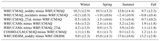
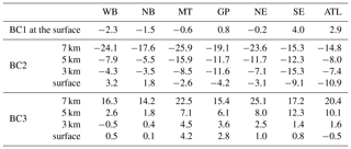
Table 3 Differences in seasonal averaged DM8A BCT (ppb) between simulations after averaging over all land grid cells over the analysis domain. Values in parentheses are the standard deviations of the differences between simulations over land.

For DM8A BCT, it is not surprising to find that dry deposition significantly reduces DM8A BCT for all seasons by as much as about 10 ppb averaged over the US (Table 3). Sub-grid cloud mixing in general slightly increases DM8A BCT (Table 3) because the sub-grid cloud mixing in CMAQ tends to mix the air aloft (e.g., above the PBL), which is richer in BCT (especially BC2), downward into the PBL. This is later confirmed by results on the relative contributions of tracers. The largest impact of sub-grid cloud mixing is found in summer, with increases in DM8A BCT of over 2.5 ppb across the eastern US and the Atlantic Ocean. In spring and fall, the impact is generally smaller but not negligible, as increases in DM8A BCT still exceed 1 ppb regionally. In winter, the impact is less than 1 ppb across the US. Lastly, for wet scavenging, little change in DM8A BCT (less than 0.1 ppb for domain average) is found so that the impact of this process on the simulated inert tracers is negligible for WRF∕CMAQ and is not shown. In addition, the impact of the three processes is relatively uniform across the US, as small deviations are found (summarized in Table 3).

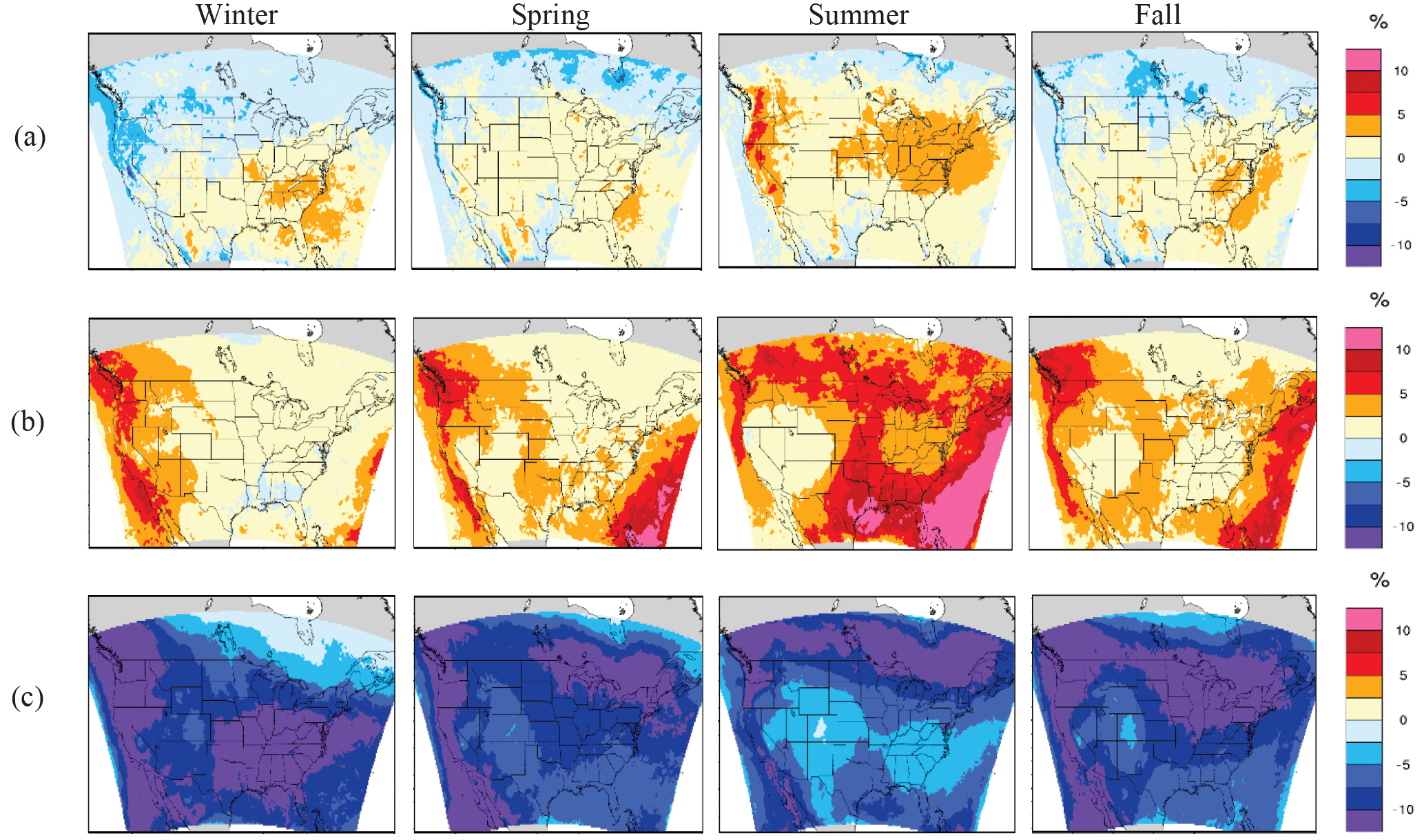
Figure 3 Differences in the seasonal averaged DM8A BC1∕BCT (%) between WRF∕CMAQ_noddry and WRF∕CMAQ (a), between WRF∕CMAQ_nocldmix and WRF∕CMAQ (b), and between WRF∕CMAQ_27aL and WRF∕CMAQ (c). All results are shown as sensitivity simulation minus WRF∕CMAQ. The areas in white or grey are the grid cells that are out of the simulation domain of WRF∕CMAQ.

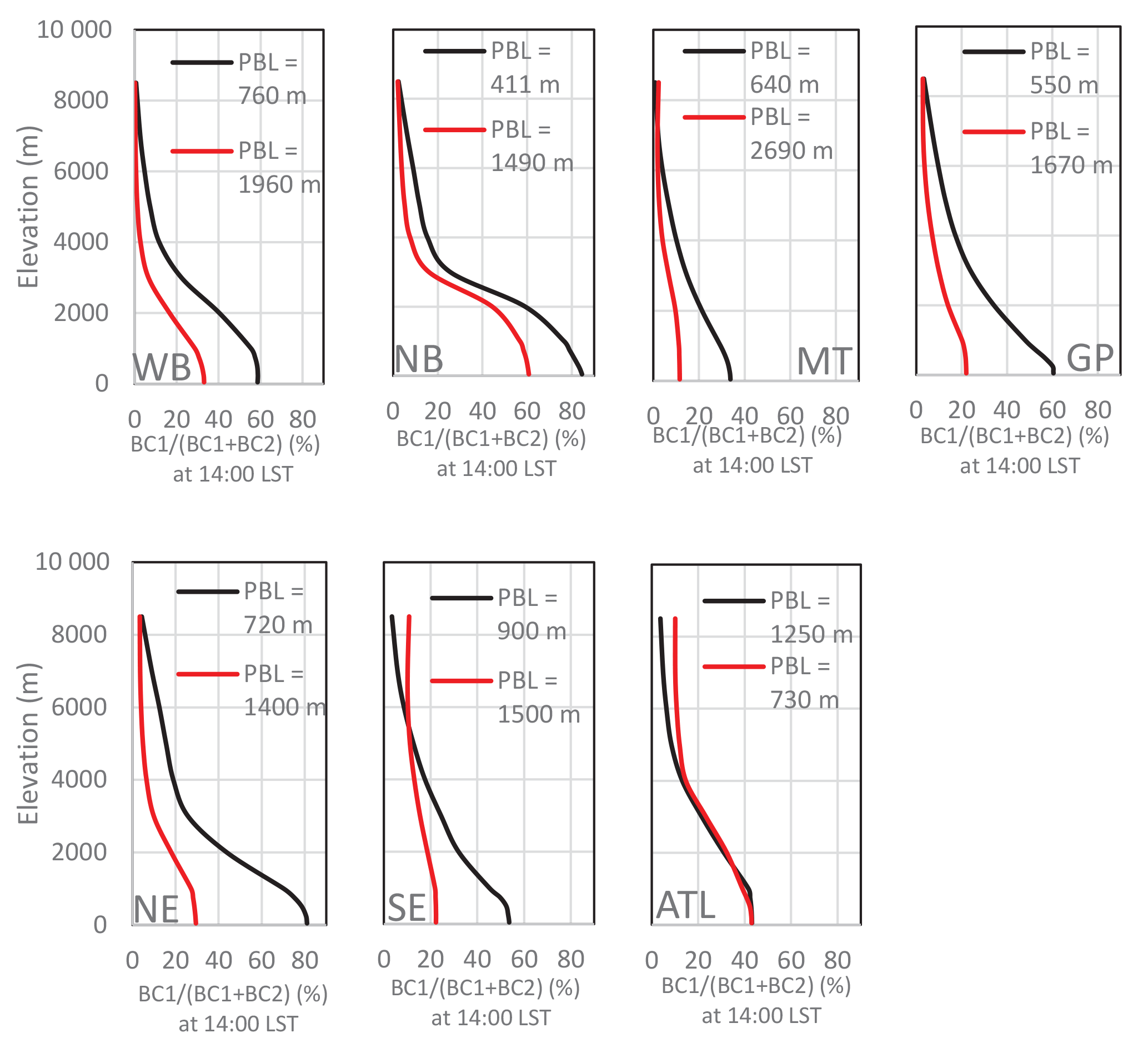
Figure 4 Seasonal averaged vertical profiles of $\text{BC1}/(\text{BC1}+\text{BC2})$ (in percentage) for WRF∕CMAQ in winter (in black) and in summer (in red) over the subregions at their local standard time of 14:00. The numbers in the legend show the seasonal averaged maximum PBL height during the daytime over each subregion.

For the relative contributions of inert tracers, only the differences in DM8A BC1∕BCT between WRF∕CMAQ and its sensitivity simulations are shown (Fig. 3) to illustrate the changes in the relative contributions of inert tracers at the surface, as the changes in DM8A BC1∕BCT and in DM8A BC2∕BCT are usually the same in magnitude with opposite sign. The changes in DM8A BC3∕BCT are less than 0.5 % domain-wide in all seasons, except for the differences between WRF∕CMAQ and WRF∕CMAQ_nocldmix in summer, which will be discussed later. The impact of dry deposition is usually within ±5 % and the direction of the change varies with space and time. At the surface, the removal of inert tracers is proportional to the absolute mixing ratios of each tracer, which in turn will be updated through vertical mixing in the PBL. In other words, the process of dry deposition does not modify the relative contributions of inert tracers directly, but through vertical turbulent mixing. Therefore, in regions where the vertical gradient of the tracer is steeper within the PBL, a larger impact of dry deposition on the DM8A BC1∕BCT is expected. To confirm this hypothesis, the seasonal averaged vertical profiles of $\text{BC1}/(\text{BC1}+\text{BC2})$ and the maximum daytime PBL height in WRF∕CMAQ are examined in each subregion at 14:00 (local standard time) (Fig. 4). For example, in WB and NE subregions, the change in $\text{BC1}/(\text{BC1}+\text{BC2})$ from the surface to the top of the PBL is larger in summer than winter, which is consistent with the larger differences seen in DM8A BC1∕BCT between WRF∕CMAQ_noddry and WRF∕CMAQ during summer than winter (Fig. 3a). In contrast, the change in $\text{BC1}/(\text{BC1}+\text{BC2})$ from the surface to the top of the PBL is larger in winter than summer in SE and ATL, which is consistent with the larger impact of dry deposition over these two regions in winter. In addition to the vertical gradient of $\text{BC1}/(\text{BC1}+\text{BC2})$, the magnitude and direction for the change in $\text{BC1}/(\text{BC1}+\text{BC2})$ at the surface also depends on the amount of air exchanged between the surface and aloft. Therefore, the impact of dry deposition on $\text{BC1}/(\text{BC1}+\text{BC2})$ varies in season and space.

The sensitivity to sub-grid cloud mixing shows that it always tends to decrease DM8A (BC1∕BCT) and increase DM8A (BC2∕BCT) (Fig. 3b), leading to slightly higher DM8A BCT in WRF∕CMAQ than WRF∕CMAQ_nocldmix (Table 3). The largest impact is found in summer, when convection is most active and frequent, especially over the Gulf Coast area and the Atlantic Ocean with a change in DM8A BC1∕BCT of about 10 % and in DM8A BCT of about 2.5–5 ppb. In other seasons, sub-grid cloud mixing mainly affects the western coastal area and the oceans with its impact on the other areas across the US usually less than 1.0 ppb in DM8A BCT and less than 5 % in DM8A BC1∕BCT. For wet scavenging, it is found that its impact on the relative contributions of tracers is also negligible, with differences in DM8A BC1∕BCT less than 0.1 % domain-wide in all seasons (not shown). In addition to these three processes, vertical grid structure is also an important model configuration in CTMs as it affects the vertical transport of inert tracers and the attribution of LB ozone to inert tracers. Comparing WRF∕CMAQ with WRF∕CMAQ_27aL shows that the coarser vertical structure in the free troposphere only slightly increases DM8A BCT (Table 3) but significantly modifies the relative contributions of BC1 and BC2 at the surface (Fig. 3c).

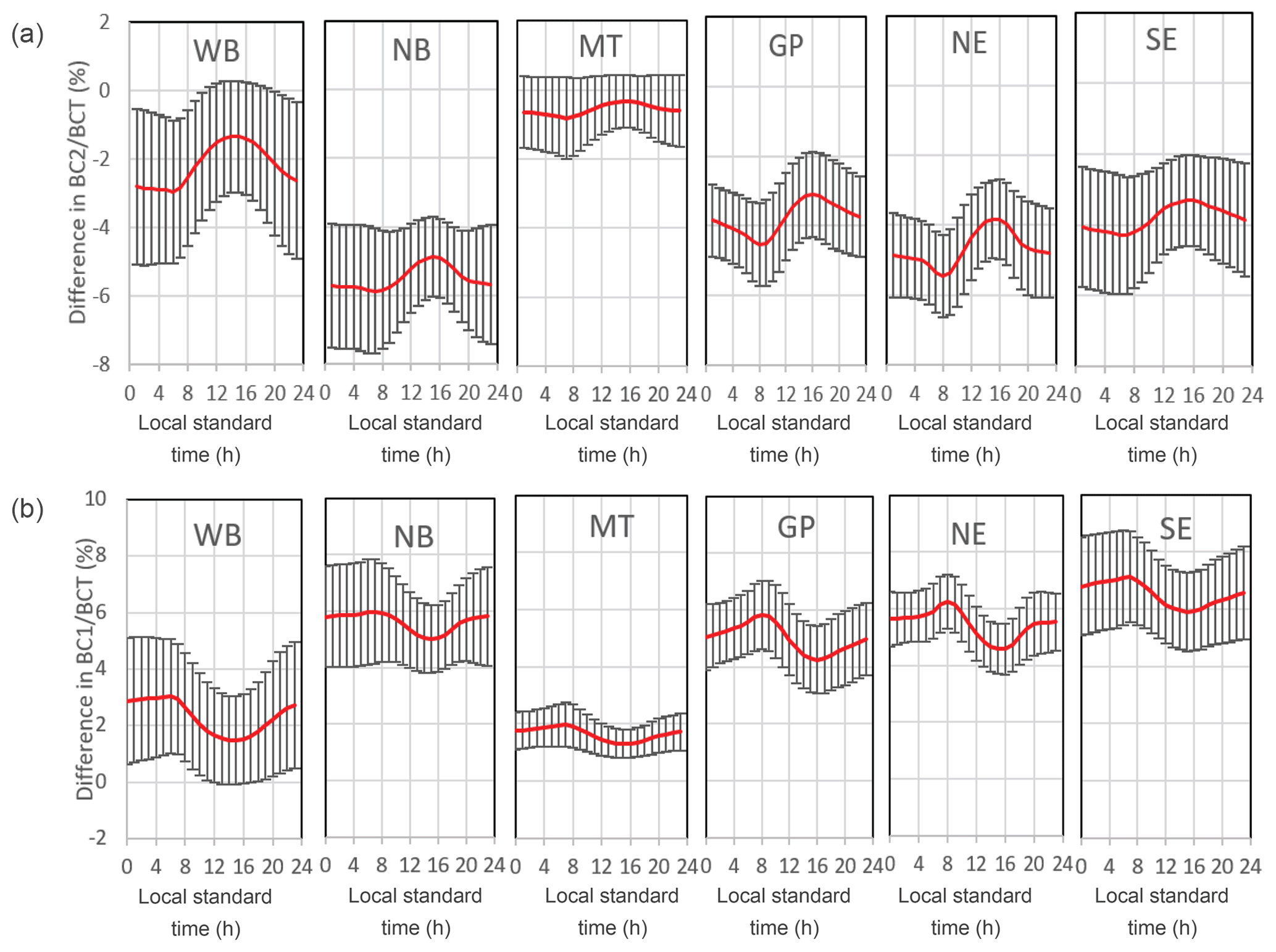
Figure 5 Diurnal cycles for the differences in BC2∕BCT (%) (a) and in BC1∕BCT (%) (b) between WRF∕CMAQ_nocldmix and WRF∕CMAQ (WRF∕CMAQ_nocldmix minus WRF∕CMAQ) during summer over subregions. For each subregion, the regional average is represented by a red line with the standard deviation in black bars.

As mentioned, the impact of a given physical process in CTMs on LB ozone at the surface may not be isolated from other physical processes. In this study, vertical turbulent mixing could also be involved in determining the differences in inert tracers at the surface between WRF∕CMAQ and its sensitivity simulations discussed above. To investigate the impact of vertical turbulent mixing in conjunction with the physical treatment discussed above, the diurnal cycles of the differences in BC1∕BCT and BC2∕BCT at the surface are examined between WRF∕CMAQ and its sensitivity simulations. The results for summer, when the largest diurnal variance usually occurs, are shown in Fig. 5. The diurnal change in the differences in BC1∕BCT is generally much smaller than the diurnally averaged differences in BC1∕BCT between WRF∕CMAQ and WRF∕CMAQ_nocldmix and between WRF∕CMAQ and WRF∕CMAQ_27aL over all subregions (Table 5), suggesting that the impact of sub-grid cloud mixing and vertical resolution on the relative contributions of inert tracers at the surface is in general much stronger than the impact of diurnal variability in vertical mixing. In contrast, the magnitude of the diurnal variance in the difference in BC1∕BCT exceeds the diurnally averaged difference in BC1∕BCT in the subregions of WB and NB between WRF∕CMAQ and WRF∕CMAQ_noddry (Table 5), suggesting a stronger dependence of the dry deposition process on vertical turbulent mixing in determining the inert tracers at the surface. Similar results are found for BC2∕BCT (not shown). There is no obvious pattern in the diurnal variance in the differences in the relative contributions of inert tracers, except for the model pair of WRF∕CMAQ and WRF∕CMAQ_nocldmix. In summer, for example, their differences in BC2∕BCT and BC1∕BCT (WRF∕CMAQ_nocldmix minus WRF∕CMAQ) always decrease during daytime (Fig. 5). This is because sub-grid cloud mixing becomes less effective in reducing the vertical gradient of inert tracers in daytime due to stronger turbulent mixing in daytime than nighttime.

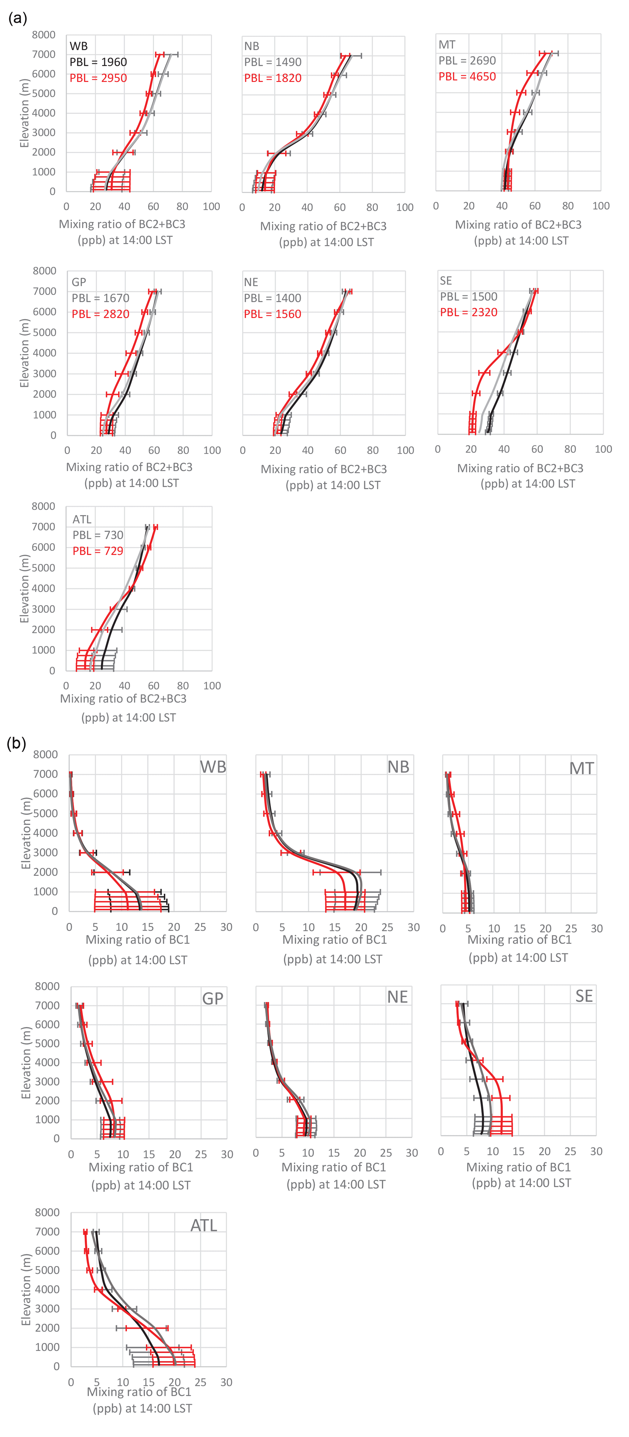
Figure 6 (a) Seasonal averaged vertical profiles of (BC2+BC3) (in ppb) for WRF∕CMAQ (black), WRF∕CMAQ_nocldmix (grey), and COSMO-CLM∕CMAQ (red) in summer over the subregions at their local standard time of 14:00. The bars represent the standard deviations over the subregion (the standard deviations of WRF∕CMAQ_nocldmix are not shown, as the values are almost the same as those of WRF∕CMAQ). The numbers in the legend are the seasonal averaged maximum PBL height during the daytime over each subregion for WRF∕CMAQ (in black) and for COSMO-CLM∕CMAQ (in red).(b) Same as (a), but for BC1 (in ppb).

Lastly, the sum of the differences in BC1∕BCT and BC2∕BCT at the surface is approximately zero between WRF∕CMAQ and WRF∕CMAQ_noddry and between WRF∕CMAQ and WRF∕CMAQ_27aL over all subregions in all seasons. For WRF∕CMAQ_nocldmix and WRF∕CMAQ, especially in summer, the differences in BC1∕BCT and BC2∕BCT do not add up to zero in the MT, GP, NE, and SE subregions (Fig. 5) due to the negative differences in BC3∕BCT. This result suggests that sub-grid cloud mixing also transports more BC3 downward through deep convection at high altitude. For example, the vertical profiles of BC2+BC3 from the two simulations clearly show that the mixing ratio of BC2+BC3 in WRF∕CMAQ is higher than that in WRF∕CMAQ_nocldmix from the altitude ∼3–4 km in the MT, GP, and NE regions and from ∼5–6 km in SE (Fig. 6a). In WB and NB, however, the mixing ratio of BC2+BC3 in WRF∕CMAQ does not exceed that in WRF∕CMAQ_nocldmix until about 2 km (Fig. 6a), so sub-grid cloud mixing has little impact on the vertical transport of BC3 and the differences in BC1∕BCT and BC2∕BCT almost add up to zero (Fig. 5).

3.2 WRF∕CAMx vs. WRF∕CMAQ

This model pair has some important features in common, which the other model pairs do not. The two models used the same meteorological inputs for CTMs and were configured with the same horizontal resolution, so there should be little difference in 3-D advection. Meanwhile, the two models use different representations for the other important physical processes that the inert tracers undergo, including vertical turbulent mixing, dry and wet deposition, and sub-grid cloud mixing (Table 1).

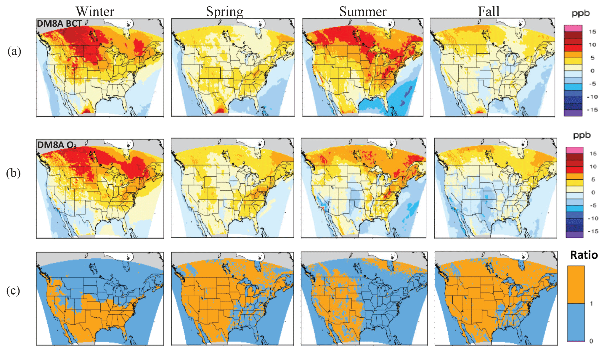
Figure 7 Differences in the seasonal averaged DM8A BCT (in ppb, a) and DM8A O₃ (b) between WRF∕CAMx and WRF∕CMAQ (WRF∕CAMx minus WRF∕CMAQ) in the analysis domain. (c) The seasonal averaged ratio of dry deposition velocity (WRF∕CAMx over WRF∕CMAQ) for ozone. The areas in white or grey are the grid cells that are out of the simulation domain.

The model differences in DM8A BCT are relatively small (within ±5 ppb) in spring and fall. In winter and summer, however, the differences can reach as much as 7.5–10 ppb regionally (Fig. 7a). The results demonstrate that physical treatment in CTMs serves as an important source of uncertainty when estimating the impact of LB ozone on ozone level at the surface aside from the meteorological inputs and the lateral boundary conditions. Differences in DM8A O₃ and DM8A BCT between WRF∕CMAQ and WRF∕CAMx show strong spatial correlations with similar magnitudes except for summer (Fig. 7b). Two processes lead to weaker agreement between the difference in inert tracers and the difference in ozone in summer. First, chemical decay due to the photolysis of LB ozone is the strongest in summer and not represented by inert tracers. Second, the chemical formation of ozone peaks in summer. The results suggest that the impact of physical treatment can compete or even overwhelm the impact of chemistry on the LB ozone reaching the surface in some cases. There are significant differences in the relative contributions of BC1 and BC2 at the surface in all seasons, which are usually much larger than the differences found in BC3∕BCT (within in 2.5 %) in all seasons. Hence, only the results in DM8A BC1∕BCT are shown for this model pair (Fig. 8a) to illustrate the model differences in the relative contributions of inert tracers at the surface.

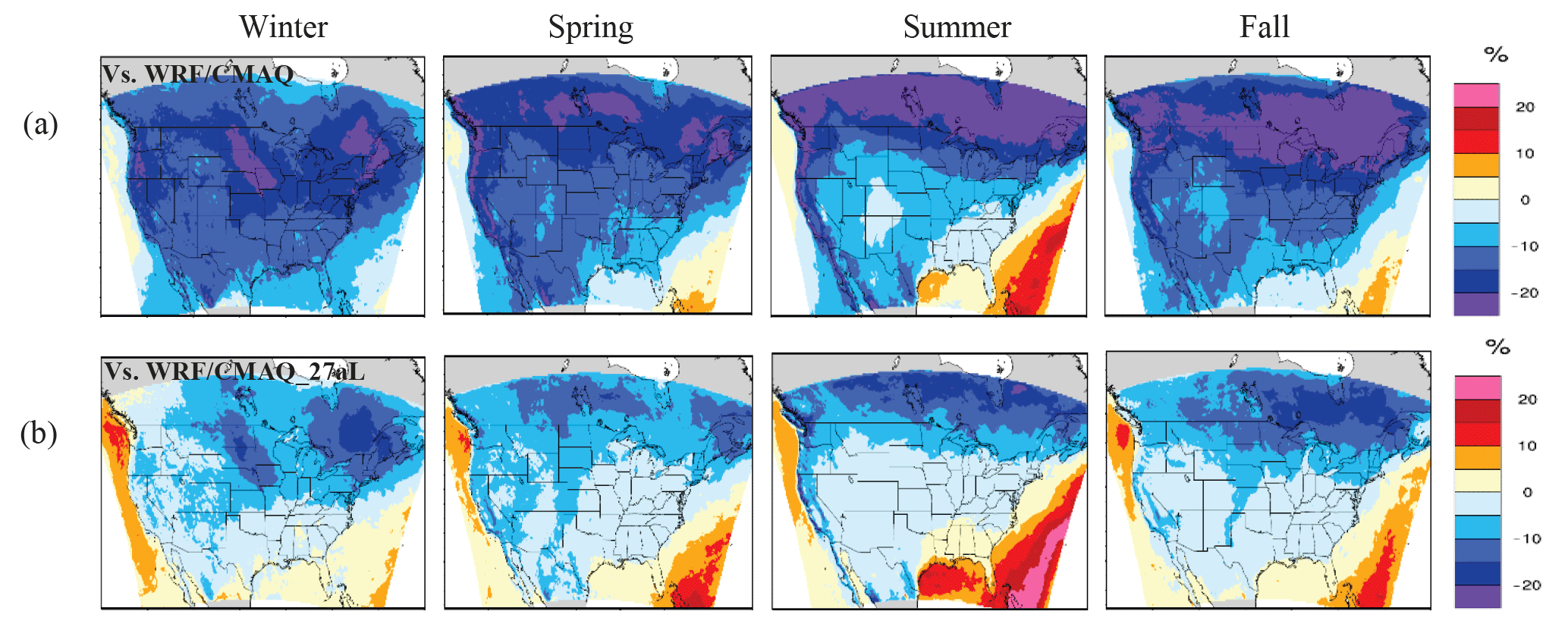
Figure 8 Differences in the seasonal averaged DM8A BC1∕BCT (%) between WRF∕CAMx and WRF∕CMAQ (WRF∕CAMx minus WRF∕CMAQ) (a) and between WRF∕CAMx and WRF∕CMAQ_27aL (WRF∕CAMx minus WRF∕CMAQ_27aL) (b) in the analysis domain.

The impact of vertical grid structure on the model differences is first examined by comparing WRF∕CAMx minus WRF∕CMAQ with WRF∕CAMx minus WRF∕CMAQ_27aL. For DM8A BCT, about 10 %, 60 %, 20 %, and 40 % of the difference between WRF∕CAMx and WRF∕CMAQ over land can be attributed to the difference in vertical resolution in winter, spring, summer, and fall, respectively (Table 3). For the relative contributions of inert tracers, about 60 % of the differences in DM8A BC1∕BCT between WRF∕CAMx and WRF∕CMAQ over land can be attributed to their differences in vertical resolution in all seasons (Fig. 8b; Table 4).

Table 4 Differences in seasonal averaged DM8A BC1∕BCT (%) between simulations after averaging over all land grid cells over the analysis domain. Values in parentheses are the standard deviations of the differences between simulations over land.

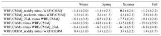
Table 5 Differences in BC1∕BCT (%) averaged over 24 h in the diurnal cycle over seven subregions in summer between WRF∕CMAQ and its sensitivity simulations and between WRF∕CAMx and WRF∕CMAQ_27aL. The numbers in parentheses represent the range of the diurnal differences in BC1∕BCT (%), namely the maximum minus the minimum within the diurnal cycle of the difference in BC1∕BCT.

As to the impact of other physical processes on the model differences, while the wet deposition of inert tracers is not represented in WRF∕CAMx, our analysis for WRF∕CMAQ and its sensitivity simulations in the previous section has shown that the impact of wet deposition is negligible in WRF∕CMAQ, and therefore the absence of this process in WRF∕CAMx should not be a significant contributor to the model differences in inert tracers. The impact of sub-grid cloud mixing in WRF∕CMAQ is usually pronounced over ocean and coastal regions with an average change of less than 1 ppb in DM8A BCT over land except during summer (Table 3). Sub-grid cloud mixing in WRF∕CMAQ also always decreases BC1∕BCT and increases BC2∕BCT at the surface. Although WRF∕CAMx does not represent this process, the DM8A BC1∕BCT in WRF∕CAMx is usually lower than that in WRF∕CMAQ_27aL (Fig. 8b) over land. Therefore, the remaining differences between WRF∕CAMx and WRF∕CMAQ_27aL do not result from wet scavenging or sub-grid cloud mixing. To investigate the impact of dry deposition on DM8A BCT, the seasonal averaged dry deposition velocity at the surface is compared between the two models, and a correlation is seen between the differences in BCT and the differences in dry deposition velocity. The differences in BCT (WRF∕CAMx minus WRF∕CMAQ; Fig. 7a) tend to increase when and where the dry deposition velocity in WRF∕CAMx is smaller (Fig. 7c). For example, in winter, the difference in DM8A BCT in the north is about 5 ppb higher than that in the south, with a lower dry deposition velocity found in WRF∕CAMx over the northern part of the domain. Similar results also are seen in summer. In addition, the spatial distributions of the differences in BCT are more uniform in spring and fall than those in winter and summer and, correspondingly, the spatial distributions of the ratio of dry deposition velocity are also more uniform in spring and fall. Therefore, we believe that the large spatial gradient of the difference in DM8A BCT in winter and summer between the two models is primarily due to their differences in dry deposition.

However, dry deposition does not explain the higher DM8A BCT in WRF∕CAMx when the dry deposition velocity in WRF∕CAMx is also faster, such as in spring. In addition, the remaining model difference in the relative contributions of inert tracers at the surface (as shown in Fig. 8b) cannot be explained by the difference in dry deposition alone because, as mentioned above, dry deposition modifies the relative contributions of inert tracers at the surface through vertical turbulent mixing with relatively small changes in the relative contributions of inert tracers at the surface. Therefore, the remaining differences in inert tracers at the surface can only be explained by their difference in vertical turbulent mixing. WRF∕CMAQ used the parameterization ACM2 (Pleim, 2007), while WRF∕CAMx used “K theory” (Table 1). Under neutral and stable conditions, both parameterizations can adequately characterize vertical mixing (Ramboll, 2018), while during periods of deep vertical convection, K theory is less efficient in the mixing of the convective boundary layer (Ramboll, 2018). However, our results indicate that WRF∕CAMx always tends to have stronger vertical turbulent mixing than WRF∕CMAQ. On the one hand, as shown in Fig. 7, DM8A BCT in WRF∕CAMx is higher than that in WRF∕CMAQ even when the dry deposition velocity in WRF∕CAMx is faster, indicating that more air aloft (with richer BCT) is brought downward to compensate for the loss of inert tracers. On the other hand, the DM8A BC1∕BCT in WRF∕CAMx is always lower than that in WRF∕CMAQ over land (Fig. 8b) with correspondingly higher DM8A BC2∕BCT (not shown), again suggesting that WRF∕CAMx mixes more air from aloft (with lower BC1∕BCT and higher BC2∕BCT) downward than WRF∕CMAQ. In addition, the NB subregion usually shows larger differences in DM8A BC1∕BCT than other regions (Fig. 8b). This is because the vertical gradients of BC2+BC3 and BC1 in NB from the surface to 3 km are usually steeper than the gradients in other regions in WRF∕CMAQ (e.g., in summer, as shown in Fig. 6a, b), so the stronger vertical mixing in WRF∕CAMx tends to have a larger impact on inert tracers at the surface in this region. The stronger vertical mixing in WRF∕CAMx also compensates for the lack of sub-grid cloud mixing to a certain extent, leading to smaller differences in DM8A BCT and DM8A BC1∕BCT, especially over the SE and the Gulf Coast region during summer.

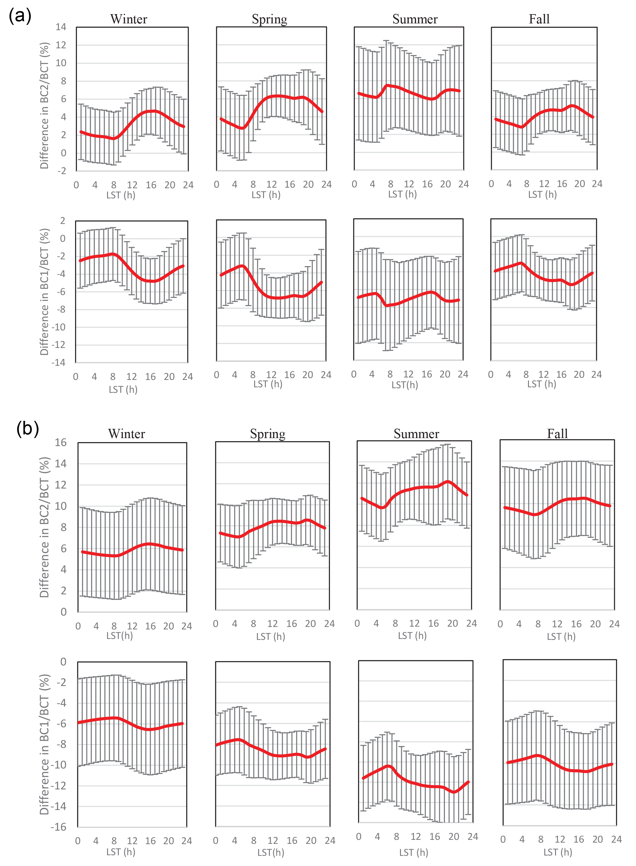
Figure 9 (a) Differences in the seasonal averaged diurnal cycles of BC2∕BCT (in percentage) and in BC1∕BCT (in percentage) between WRF∕CAMx and WRF∕CMAQ_27aL (WRF∕CAMx minus WRF∕CMAQ_27aL) over the WB subregion. For each season and hour, the regional average is shown in red with the standard deviation shown in black bars. Panel (b) is the same as (a), but over the NB subregion.

To further illustrate the role of differences in vertical mixing between the two models, the diurnal cycles of the differences in BC1∕BCT and BC2∕BCT between WRF∕CAMx and WRF∕CMAQ_27aL are examined over the subregions. Little variance (less than 1 %) is found over most of the subregions, except that a clear diurnal change is noticed over WB and NB in most seasons. Over these two regions, the differences in BC2∕BCT and BC1∕BCT (Fig. 9a, b) grow from night to daytime as the vertical turbulent mixing becomes stronger.

To summarize, 10 % to 60 % of the seasonal averaged differences in inert tracers between WRF∕CMAQ and WRF∕CAMx at the surface can be attributed to their difference in the vertical grid structure in the free troposphere. Vertical turbulent mixing primarily contributes to the remaining differences across the entire land in all seasons. Stronger vertical mixing in WRF∕CAMx brings more BC2 downward, leading to higher DM8A BCT and BC2∕BCT at the surface in WRF∕CAMx. The differences in inert tracers due to vertical mixing are partially counteracted by their difference in sub-grid cloud mixing over the SE and the Gulf Coast region during summer. The process of dry deposition adds extra gradients to the spatial distribution of the differences in DM8A BCT by about 5–10 ppb during winter and summer. Unfortunately, it is impossible to further quantitatively attribute the model differences in inert tracers to the processes of dry deposition and vertical turbulent mixing with the sensitivity simulations available in this study.

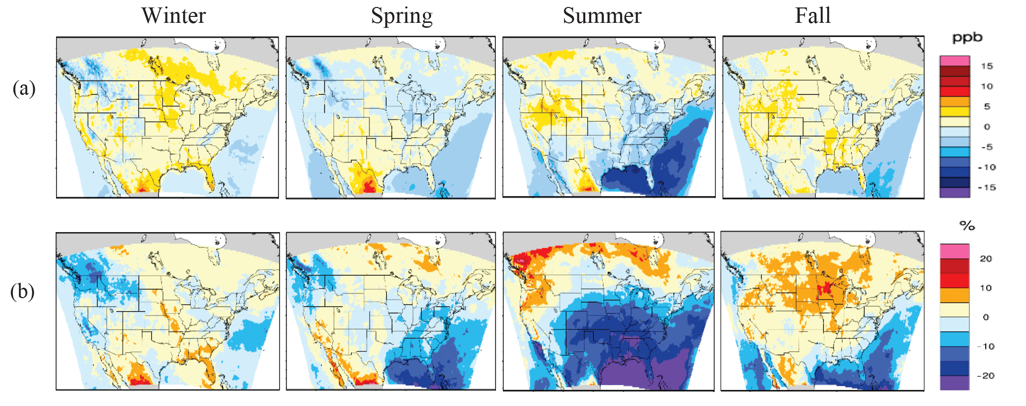
Figure 10 Differences in the seasonal averaged DM8A BCT (in ppb, a) and DM8A BC2∕BCT (in percentage, b) between COSMO-CLM∕CMAQ and WRF∕CMAQ (COSMO-CLM∕CMAQ minus WRF∕CMAQ) in the analysis domain. The areas in white or grey are the grid cells that are out of the simulation domain of either of the two models.

3.3 COSMO-CLM∕CMAQ vs. WRF∕CMAQ

Unlike the model pair in the previous section, COSMO-CLM∕CMAQ and WRF∕CMAQ do not share the same meteorological inputs; however, the same physical parameterizations are used in CMAQ to represent the processes that inert tracers undergo (Table 1). Furthermore, the two models have similar vertical resolution from the surface up to about 400 hPa (Fig. 2), which covers the majority of the pressure range for BC1 and BC2. The differences in DM8A BCT and the relative contributions of inert tracers for this model pair are usually much smaller than the differences between WRF∕CAMx and WRF∕CMAQ. For example, the differences in DM8A BCT are within 2.5 ppb (Table 3; Fig. 10a) across most of the US. The results indicate that the uncertainty stemming from physical treatment in CTMs may rival or exceed the uncertainty from meteorological inputs, especially when nudging is applied to generate the meteorological fields (Table 1) with constraints above the PBL at synoptic scales. The largest differences at the surface occur in the summer over the SE and ATL subregions with lower DM8A BCT in COSMO-CLM∕CMAQ by about 5 and 10 ppb, respectively. This is because the large difference in BC2 is not offset by the difference in BC1 or BC3 as in other regions (Table 6). The physical process(es) contributing to the large differences over the two areas will be discussed later.

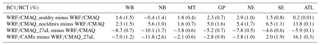
Table 6 Seasonally averaged differences between COSMO-CLM∕CMAQ and WRF∕CMAQ (COSMO-CLM∕CMAQ minus WRF∕CMAQ) in BC1 (ppb) at the surface, in BC2 (ppb) and BC3 (ppb) at the surface, and at a specific elevation (above ground level) in summer at 14:00 LST over seven subregions.

The difference in the relative contributions of inert tracers at the surface is dominated by the difference in DM8A BC1∕BCT and DM8A BC2∕BCT over most regions in all seasons, except MT, GP, and NE in summer, when the differences in DM8A BC2∕BCT and in DM8A BC3∕BCT dominate (Table 6). Therefore, the model differences in DM8A BC2∕BCT are shown to demonstrate the model differences in the relative contributions of inert tracers (Fig. 10b). The difference in DM8A BC2∕BCT is in general small (within 5 %) over most of the US, except during the summer. In summer, the large differences in DM8A BC2∕BCT over MT and GP result from their differences in BC2 and BC3 at the surface (Table 6) due to their difference in vertical resolution above 400 hPa. Over SE and ATL, however, the large differences in BC2∕BCT result from their difference in BC2 alone at the surface, suggesting the impact of physical processes other than vertical resolution in these two regions.

In SE and ATL during summer, COSMO-CLM∕CMAQ shows much larger vertical gradients in BC1 and in BC2+BC3 than WRF∕CMAQ from 5 to 3 km (Fig. 6a, b). Of all the physical processes that inert tracers undergo, sub-grid cloud mixing and horizontal transport may contribute to the large difference in vertical gradient at this altitude range. Separate analysis reveals that the precipitation over the southeastern US, which is mainly convective rain in summer given the horizontal resolution of the simulations, is smaller in COSMO-CLM∕CMAQ than in WRF∕CMAQ (not shown), suggesting weaker sub-grid cloud mixing in COSMO-CLM∕CMAQ. By comparing the vertical profiles of WRF∕CMAQ_nocldmix and COSMO-CLM∕CMAQ, similar vertical gradients in BC2+BC3 and BC1 are found between these two simulations in ATL. The results confirm that much less BC2 is mixed downward from 3–5 km into the PBL in COSMO-CLM∕CMAQ, and the difference in BC2 cannot be compensated for by the differences in BC1 and BC3, leading to the large negative differences in BCT at the surface between the two models. In SE, however, the vertical gradient in COSMO-CLM∕CMAQ from 5 to 3 km is still larger than that in WRF∕CMAQ_nocldmix, which is likely due to the differences in horizontal advection between COSMO-CLM∕CMAQ and WRF∕CMAQ.

In general, the two models show similar vertical profiles of BC1 and BC2+BC3 over the subregions through all seasons, which again suggests similarity between the two models at the process level. The vertical profiles in summer are shown (Fig. 6a, b) and discussed as the largest differences in inert tracers are found in summer both at the surface and aloft. Furthermore, the vertical profiles suggest the potential compensation between different physical processes in this season over certain subregions, leading to small differences in DM8A BCT at the surface. In WB and NB, BC2+BC3 in COSMO-CLM∕CMAQ begins to exceed that in WRF∕CMAQ from about 2 km, which can be due to its stronger vertical turbulent mixing as suggested by PBL height (Fig. 6a). However, BC1 in COSMO-CLM∕CMAQ is lower than WRF∕CMAQ at any altitude (Fig. 6b), suggesting that the difference in BC1 at the surface (about 2.3 ppb) is not dominated by their difference in vertical turbulent mixing, but by their difference in dry deposition. Though COSMO-CLM∕CMAQ also tends to remove more BC2+BC3 at the surface by dry deposition, the BC2+BC3 at the surface is compensated for by mixing more air aloft downward through its stronger vertical turbulent mixing. One thing to point out is that different parameterizations are used to diagnose PBL height in their simulations for meteorology, with ACM2 in WRF and an extended MYJ scheme (Doms et al., 2011) in COSMO-CLM, so that the PBL height can be defined differently. However, as a very large difference in PBL height is seen here between the two models, PBL height is a reasonable factor to suggest the potential difference in their vertical turbulent mixing. Similarly, in GP, the BC1 in COSMO-CLM∕CMAQ is always higher than that in WRF∕CMAQ (Fig. 6a), suggesting weaker dry deposition. At the same time, the less efficient removal at the surface helps to decrease the difference in BC2+BC3 at the surface, since less BC2+BC3 in COSMO-CLM∕CMAQ is available aloft (Fig. 6b) in this region. As a result, the difference in BC2+BC3 decreases from 3 km to the surface. Conversely, in MT, BC2+BC3 in COSMO-CLM∕CMAQ is lower than WRF∕CMAQ until about 2 km, while BC1 shows the opposite. The results suggest that the differences in inert tracers over MT are dominated by the stronger vertical mixing in COSMO-CLM∕CMAQ alone rather than by other physical processes. The MT region may also influence its neighboring region through horizontal advection, leading to the slight increase in the difference in BC2+BC3 and in BC1 over GP from 7 to 3 km.

To summarize, the two models show similar vertical profiles of BC1 and BC2+BC3 over subregions across most seasons, which suggests similarity between the two models at process level. The largest differences are noted during summer. The different attributions of LB ozone to BC2 and BC3 between the two models in general have a small impact on DM8A BCT at the surface, with the largest difference in DM8A BC2+BC3 of about 2.0 ppb found in summer over MT, GP, and NE. At the same time, the different attributions of BC2 and BC3 significantly change the relative contributions of BC2 and BC3 at the surface over the three regions. The results are similar to what is found between WRF∕CMAQ and WRF∕CMAQ_27aL in which the attributions of LB ozone to BC1 and BC2 are significantly different. The model differences in sub-grid cloud mixing play a primary role in their large differences in DM8A BCT and DM8A BC2∕BCT over ATL and SE in summer. Our analysis also suggests model differences in vertical turbulent mixing over most of the domain and in dry deposition over certain subregions in summer. However, the impact of different dry deposition on inert tracers at the surface is almost offset by the model difference in vertical turbulent mixing on inert tracers.

3.4 WRF∕DEHM vs. WRF∕CMAQ

Given the different simulation domains between the two models, the results cannot be compared directly to investigate the impact of physical treatment on inert tracers. However, the model sensitivity of inert tracers at the surface to the process of dry deposition can be compared between WRF∕CMAQ and WRF∕DEHM using the sensitivity simulations denoted WRF∕CMAQ_noddry and WRF∕DEHM_noddry in Table 2. The impact of dry deposition on DM8A BCT in WRF∕DEHM is about 50 % higher than that in WRF∕CMAQ except during winter (Table 3). Such large differences are not surprising given that neither the meteorological inputs nor the parameterizations are the same for the process of dry deposition between the two models (Table 1). However, both models show similar magnitudes in their changes in the relative contributions of inert tracers at the surface. For both WRF∕CMAQ and WRF∕DEHM, since little change is found in DM8A BC3∕BCT (less than 0.5 % across the entire US in all seasons), only the results in DM8A BC1∕BCT are shown to illustrate the model sensitivity of the relative contributions of inert tracers at the surface to the process of dry deposition. For both models, the sensitivity of DM8A BC1∕BCT is in general small (Table 4), with a change of less than 5 % in all seasons across the US. However, the spatial distributions of the change in DM8A BC1∕BCT are very different between the two models. The change in DM8A BC1∕BCT in WRF∕CMAQ (Fig. 3a) shows much more spatial variance than that in WRF∕DEHM (Fig. 11), suggesting differences in the vertical profiles of inert tracers and differences in the process of turbulent mixing between the two models.

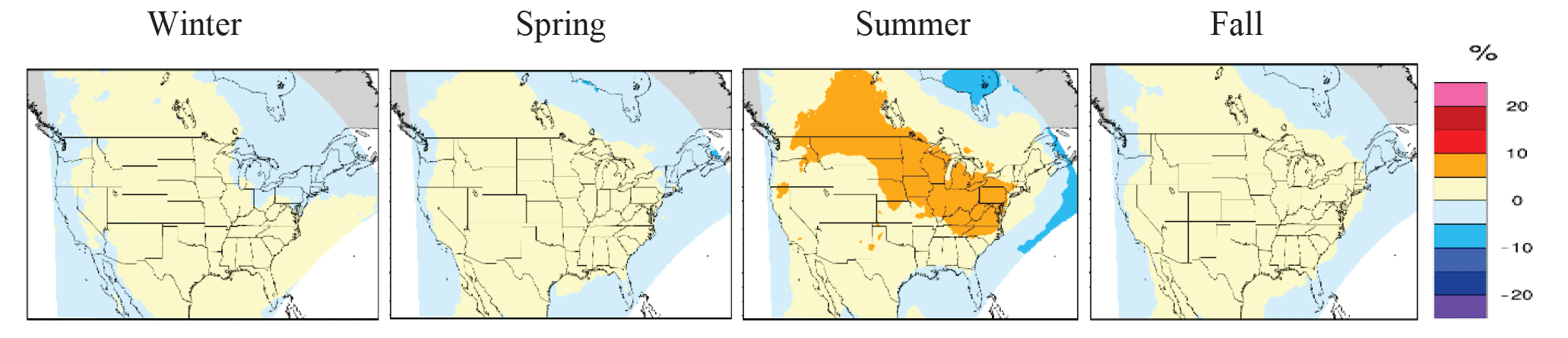
Figure 11 Differences in the seasonal averaged DM8A BC1∕BCT (%) between WRF∕DEHM_noddry and WRF∕DEHM (WRF∕DEHM_noddry minus WRF∕DEHM). The areas in white or grey are the grid cells that are out of the simulation domain of WRF∕DEHM.

4 Summary and discussion

This study investigated the impact of physical treatment in CTMs on lateral boundary (LB) ozone reaching the surface across the US with the implementation of inert tracers for LB ozone. The differences in inert tracers at the surface between different models are attributed to model differences at the process level.

The analysis focused on intercomparing three models with each other, namely WRF∕CMAQ, WRF∕CAMx, and COSMO-CLM∕CMAQ. WRF∕CMAQ and WRF∕CAMx share the same meteorological inputs, but the physical processes that inert tracers undergo (other than 3-D advection) are represented differently. On the other hand, the WRF∕CMAQ and COSMO-CLM∕CMAQ simulations are driven by different meteorological fields but share the same CTM. The model differences in DM8A BCT between WRF∕CMAQ and COSMO-CLM∕CMAQ are usually found to be much smaller than those between WRF∕CMAQ and WRF∕CAMx across the US in all seasons. The results indicate that the uncertainty stemming from physical treatment in CTMs may compete or exceed the uncertainty from meteorological inputs, especially when nudging is applied to constrain the synoptic-scale meteorology above the PBL. Furthermore, the model differences in inert tracers are investigated at the process level. Different vertical resolutions and discretizations are used by the three models, leading to differences in the attributions of LB ozone to BC1, BC2, and BC3. The impact of vertical grid structure on DM8A BCT at the surface is usually small (within 1 ppb) across the US, but not negligible regionally with the seasonal averaged changes in DM8A BCT exceeding 1 ppb. At the same time, the vertical grid structure significantly modifies the relative contributions of inert tracers at the surface. These findings suggest a need for finer vertical resolution in both the free troposphere and the lower stratosphere to better represent the impact of the intercontinental transport of ozone and ozone intrusion on ozone levels at the surface. Dry deposition strongly affects the DM8A BCT at the surface in all seasons. However, its impact on the relative contributions of inert tracers is usually small even when the process is represented by different parameterization and driven by different meteorology. Sub-grid cloud mixing is found to be important in the western coastal US during winter, spring, and fall. In summer, its impact extends to the majority of the US with a significant impact on both DM8A BCT and the relative contributions of inert tracers at the surface. Wet scavenging is found to have little impact on the inert tracers at the surface.

Our analysis also indicates that there are significant differences in vertical turbulent mixing among the three models. Both WRF∕CAMx and COSMO-CLM∕CMAQ are very likely to have stronger vertical mixing than WRF∕CMAQ, with the same meteorology driving the turbulent mixing but represented by different parameterization in WRF∕CAMx and WRF∕CMAQ, and with different meteorology driving the turbulent vertical mixing but represented by the same parameterization method in COSMO-CLM∕CMAQ and WRF∕CMAQ. As to the relative contributions of inert tracers at the surface, in winter, spring, and fall, when the impact of other processes (especially the sub-grid cloud mixing) on the relative contributions of inert tracers is weak, the differences in DM8A BC1∕BCT and DM8A BC2∕BCT between COSMO-CLM∕CMAQ and WRF∕CMAQ are within 5 % across the majority of the US regions and 5 %–10 % in the remaining regions; the differences between WRF∕CAMx and WRF∕CMAQ_27aL are larger than 5 % in the majority of the US regions. The results indicate that the differences in vertical turbulent mixing between WRF∕CAMx and WRF∕CMAQ_27aL could also be greater than the differences between COSMO-CLM∕CMAQ and WRF∕CMAQ. As to the DM8A BCT at the surface, the process of dry deposition often interacts with vertical mixing in determining the inert tracers at the surface. For example, in summer, for COSMO-CLM∕CMAQ and WRF∕CMAQ, the impact of different dry deposition on inert tracers at the surface is almost compensated for by the opposite impact of the model difference in vertical turbulent mixing on inert tracers over the subregions WB and NB; for WRF∕CAMx and WRF∕CMAQ, a larger difference in DM8A BCT is noted in regions where dry deposition in WRF∕CAMx is weaker so that the difference in the simulated BCT due to vertical mixing is further enlarged.

The intercomparison of inert tracers simulated by different models also suggests that when similar estimates of the impact of lateral boundary ozone are found between different simulations, the results do not necessarily imply that agreement has been reached for the same reason, unless a careful comparison is performed at the process level to rule out the possibility of canceling process contributions. To carry out such analysis, process analysis (PA) (Jeffries and Tonnesen, 1994) is desirable for all simulations involved. Unfortunately, the PA tool is either not available or it was not invoked in the simulation, since PA was not a standard design protocol for AQMEII3. We recommend that future model intercomparison studies include the PA tool as a standard protocol to enable consistent process-level comparison. Additionally, given the important role that turbulent mixing and sub-grid cloud mixing can play in determining the inert tracers at the surface, aloft data would be extremely valuable in understanding the model difference and similarity in these processes. Therefore, future model intercomparison studies should consider more detailed and standard archiving of 3-D model information.