the Creative Commons Attribution 4.0 License.
the Creative Commons Attribution 4.0 License.
 | 26 Nov 2018
Assessing the impact of shipping emissions on air pollution in the Canadian Arctic and northern regions: current and future modelled scenarios
Stephen R. Beagley
Sophie Cousineau
Mourad Sassi
Rodrigo Munoz-Alpizar
Sylvain Ménard
Jacinthe Racine
Junhua Zhang
Jack Chen
Heather Morrison
Sangeeta Sharma
Lin Huang
Pascal Bellavance
Jim Ly
Paul Izdebski
Lynn Lyons
Richard Holt
A first regional assessment of the impact of shipping emissions on air pollution in the Canadian Arctic and northern regions was conducted in this study. Model simulations were carried out on a limited-area domain (at 15 km horizontal resolution) centred over the Canadian Arctic, using the Environment and Climate Change Canada's on-line air quality forecast model, GEM-MACH (Global Environmental Multi-scale – Modelling Air quality and CHemistry), to investigate the contribution from the marine shipping emissions over the Canadian Arctic waters (at both present and projected future levels) to ambient concentrations of criteria pollutants (O3, PM2.5, NO2, and SO2), atmospheric deposition of sulfur (S) and nitrogen (N), and atmospheric loading and deposition of black carbon (BC) in the Arctic. Several model upgrades were introduced for this study, including the treatment of sea ice in the dry deposition parameterization, chemical lateral boundary conditions, and the inclusion of North American wildfire emissions. The model is shown to have similar skills in predicting ambient O3 and PM2.5 concentrations in the Canadian Arctic and northern regions, as the current operational air quality forecast models in North America and Europe. In particular, the model is able to simulate the observed O3 and PM components well at the Canadian high Arctic site, Alert. The model assessment shows that, at the current (2010) level, Arctic shipping emissions contribute to less than 1 % of ambient O3 concentration over the eastern Canadian Arctic and between 1 and 5 % of ambient PM2.5 concentration over the shipping channels. Arctic shipping emissions make a much greater contributions to the ambient NO2 and SO2 concentrations, at 10 %–50 % and 20 %–100 %, respectively. At the projected 2030 business-as-usual (BAU) level, the impact of Arctic shipping emissions is predicted to increase to up to 5 % in ambient O3 concentration over a broad region of the Canadian Arctic and to 5 %–20 % in ambient PM2.5 concentration over the shipping channels. In contrast, if emission controls such as the ones implemented in the current North American Emission Control Area (NA ECA) are to be put in place over the Canadian Arctic waters, the impact of shipping to ambient criteria pollutants would be significantly reduced. For example, with NA-ECA-like controls, the shipping contributions to the population-weighted concentrations of SO2 and PM2.5 would be brought down to below the current level. The contribution of Canadian Arctic shipping to the atmospheric deposition of sulfur and nitrogen is small at the current level, < 5 %, but is expected to increase to up to 20 % for sulfur and 50 % for nitrogen under the 2030 BAU scenario. At the current level, Canadian Arctic shipping also makes only small contributions to BC column loading and BC deposition, with < 0.1 % on average and up to 2 % locally over the eastern Canadian Arctic for the former, and between 0.1 % and 0.5 % over the shipping channels for the latter. The impacts are again predicted to increase at the projected 2030 BAU level, particularly over the Baffin Island and Baffin Bay area in response to the projected increase in ship traffic there, e.g., up to 15 % on BC column loading and locally exceeding 30 % on BC deposition. Overall, the study indicates that shipping-induced changes in atmospheric composition and deposition are at regional to local scales (particularly in the Arctic). Climate feedbacks are thus likely to act at these scales, so climate impact assessments will require modelling undertaken at much finer resolutions than those used in the existing radiative forcing and climate impact assessments.
- Article
(11066 KB) - Full-text XML
-
Supplement
(1633 KB) - BibTeX
- EndNote


Unprecedented rates of warming are increasing the navigability of the Arctic Ocean and, subsequently, rendering this region accessible to increasing resource exploitation and the development that goes along with it. Over the past several decades, the extent of Arctic sea ice has declined. The rate of decline of late summer sea-ice cover has been particularly rapid since the beginning of this century (e.g., Serreze et al., 2007). The latest climate model simulations predict that the retreat of Arctic sea ice will continue throughout the 21st century, and that an ice-free Arctic Ocean in late summertime may be realized by the middle to the end of this century (Boé et al., 2009; Wang and Overland, 2009). The decline in Arctic sea ice has raised the prospect of increased Arctic shipping activities and the potential use of new transit routes, such as the Northern Sea Route, the Northwest Passage (NWP), and the Transpolar Sea Route (e.g., Stephenson et al., 2013; Melia et al., 2016). Pizzolato et al. (2016) conducted a coupled spatial analysis between shipping activity and sea ice using observations in the Canadian Arctic over the 1990–2015 period and found that there has been an increase in shipping activities in Hudson Strait, Beaufort Sea, Baffin Bay, and regions in the southern route of the Northwest Passage, and that the increases in shipping activity are significantly correlated with the reductions in sea-ice concentration in these regions.
Shipping is an important source of air pollutants. Emissions of exhaust gases and particles from ocean-going ships contain carbon dioxide (CO2), nitrogen oxides (NOx), carbon monoxide (CO), volatile organic compounds (VOCs), sulfur dioxide (SO2), particulate sulfate (SO4), black carbon (BC), and particulate organic matter (OM). These pollutants lead to the production of ozone (O3) and fine particulate matter (e.g., PM2.5), the latter primarily through oxidation of SO2 and the formation and production of SO4 particles, which degrade air quality. At the same time, O3 and SO4 resulting from ship emissions, along with CO2 and BC directly emitted from shipping, are also climate forcing agents which can impact the radiative balance through either direct or indirect effects. Shipping emissions also contribute to the deposition of nitrogen (N) and sulfur (S), which can impact ecosystems through acidification and eutrophication. Recent studies have suggested that around 15 % and 4 %–9 % of all global anthropogenic emissions of NOx and SO2, respectively, are from ocean-going ships (e.g., Corbett and Köhler, 2003; Eyring et al., 2005a). As most of the ship emissions occur within 400 km of coastlines, they primarily contribute to air pollution in coastal areas (e.g., Eyring et al., 2010; Viana et al., 2014; Aksoyoglu et al., 2016; Aulinger et al., 2016). However, these emissions can be transported hundreds of kilometres downwind and impact a much broader region (e.g., Eyring et al., 2010; Aulinger et al., 2016). Although Arctic marine shipping currently accounts for a small percentage of global shipping emissions, it makes a proportionally bigger impact on the environment than shipping does at lower latitudes due to the generally pristine Arctic background, particularly in the Canadian Arctic Archipelago. Furthermore, the lower troposphere in the Arctic is more isolated during summer, which is also the Arctic shipping season, due to the retreating Arctic dome, giving rise to much slower transport of pollutants from lower latitudes and more efficient removal processes (Stohl, 2006; Law and Stohl, 2007). Local sources of air pollution, such as shipping, play a more important role in determining air quality in this region during this time.
A number of studies assessing the impact of Arctic shipping emissions have been conducted in recent years. Based on the high-growth scenario projection of Eyring et al. (2005b) on future international shipping emissions (to year 2050) and assuming a fraction of the increase would occur in the Arctic, Granier et al. (2006) predicted an increase in Arctic surface O3 concentration by a factor of 2 to 3 due to the increase in ship NOx emissions. Ødemark et al. (2012) looked into short-lived climate forcers from current shipping and petroleum activities in the Arctic based on inventories developed by Peters et al. (2011) and found that radiative forcing from shipping emissions is dominated by the direct and indirect effects of sulfate from SO2 emissions during shipping season. The overall effect from shipping on radiative forcing is negative. Dalsøren et al. (2013) assessed the changes in surface concentrations of NO2, O3, SO4, BC, and organic carbon (OC) between years 2004 and 2030, based on the Arctic shipping inventories developed by Corbett et al. (2010), which take into account Arctic shipping growth, possible emission control measures, and the opening of diversion routes for shipping in the Arctic due to the expected melting of sea ice. Based on the same inventories of Corbett et al. (2010), Browse et al. (2013) investigated the impact of Arctic shipping on BC deposition at high latitudes, and found that the overall impact from Arctic shipping to total BC deposition remains low. Their results show that Arctic shipping contributes a maximum of 1.9 % to the total annual BC deposition north of 60∘ N at present levels and a maximum of 5 % at 2050 levels under a high-growth scenario. Most of these assessments were conducted using global models at coarse resolutions (e.g., ). In a recent study on cross-polar transport and scavenging of Siberian aerosols, Raut et al. (2017) found that the model simulation at a coarser horizontal resolution (i.e., 100 km instead of 40 km) was unable to resolve plume structures transported across the polar region in summer. The model performed much better at simulating cross-polar transport and processing using a finer horizontal resolution (40 km). At a regional scale, Marelle et al. (2016) used model simulations at 15 km resolution to estimate the regional impacts of shipping pollution in northern Norway during a 15-day period in July 2012, when an aircraft measurement campaign was conducted to characterize pollution originating from shipping and other local sources. Their estimate of the impact of shipping emissions on O3 production over the Norwegian coast was considerably lower than the estimate of Ødemark et al. (2012), which was based on a model simulation at a much coarser resolution (). The authors attributed the difference in estimated impact, at least in part, to the non-linear effects associated with the unrealistic instant dilution of ship NOx emissions in global models run at coarse resolutions, particularly under pristine background conditions as found in Vinken et al. (2011).
In this study, we assess the impact of emissions from marine shipping on the Canadian Arctic using an on-line comprehensive air quality forecast model, Global Environmental Multi-scale – Modelling Air quality and CHemistry (GEM-MACH), configured for the Arctic at 15 km resolution. A detailed baseline emission inventory for ships sailing in Canadian waters was developed utilizing vessel movement data for 2010 supplied by the Canadian Coast Guard (CCG) and activity-based emissions factors. Projections of Canadian Arctic marine shipping emissions to a future year (2030) were made based on two scenarios: business-as-usual (BAU) and emission controls (a.k.a., controlled). Model simulations for the Arctic shipping season were carried out, with and without the marine shipping emissions over the Canadian Arctic waters, at both the current (2010 baseline) and future (projected) levels. The contributions from Canadian Arctic shipping emissions to ambient concentrations of criteria pollutants (O3, PM2.5, NO2, and SO2), total S and N deposition, and BC loading and deposition were assessed in the context of their relevance to air quality, local ecosystems, and climate. In the following sections, we will describe the Canadian shipping emission inventories (Sect. 2) and the modelling system and simulation setup (Sect. 3). An evaluation of the 2010 baseline simulation against available observations is presented in Sect. 4, and the assessment of the impact of the Arctic shipping emissions in Sect. 5. We will end with conclusions in Sect. 6.
The 2010 Canadian national marine shipping emission inventory used for this study was generated by using the Marine Emission Inventory Tool (MEIT) developed for Environment and Climate Change Canada (ECCC) (SNC-Lavalin Environment, 2012). The inventory includes all commercial marine vessel classes tracked by the CCG within Canadian waters, as well as small commercial craft such as ferries, tugboats, and fishing vessels. All coastal area as well as inland rivers and lakes are included in the inventory. The basis for the inventory is movement data as logged in the Information System on Marine Navigation (INNAV) for eastern Canada and the Arctic and the Vessel Traffic Operator Support System (VTOSS) through CCG Vessel Traffic Services (VTS) for the west coast. INNAV data for 2010 are representative of all ocean-going vessel (OGV) movements, whereas data gaps exist in the 2010 VTOSS dataset. In addition, Pacific Pilotage Authority movement data and port-level data are also used to supplement VTOSS data as needed (SLE, 2012). The activity-based emission factors used in MEIT for processing the 2010 national inventory were specific factors appropriate for engine size (based on US EPA engine classification), speed, and fuel type (Weir Marine Engineering, 2008; SLE, 2012). Emissions were calculated on a voyage-by-voyage basis, and vessel speed and implied load on the main and auxiliary engines were evaluated by each segment of a voyage. Temporal resolution of the 2010 national marine inventory includes emissions by hour, day, and month of the year, and spatial resolution includes emissions allocated to regions of Canada (by province and many sub-regions defined in previous marine emission inventory analysis work). The Arctic portion of the 2010 national marine emission inventory was further updated to include revised main engine load factors (Innovation Maritime and SNC-Lavalin Environment, 2013). The emission inventory covers criteria air contaminants (CACs), such as NOx, sulfur oxides (SOx), CO, VOCs (including VOCs from combustion and fugitive VOCs from crude oil tankers but not fugitive VOC emissions from oil barges and other petroleum tankers), PM (as total PM, PM10, and PM2.5 as well as elemental, organic, and sulfate fractions), and ammonia (NH3), greenhouse gases (GHGs), and air toxics.
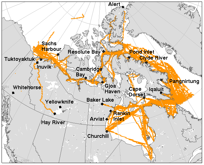
The Canadian Arctic waters defined in this study are the portion of Canadian waters excluded from the North American Emission Control Area (NA ECA), which include both coastal and inland waters north of 60∘ N, the Hudson Bay, and James Bay (see Fig. 1). Canada's Arctic waters (particularly in the high Arctic) are characterized by variable ice conditions and extreme weather. The vastness and remoteness of the region further contribute to the challenges that shippers are faced with when sailing through these waters. Even during the summer months when ice levels are at their lowest, ships must ensure that they have ice-strengthened hulls or be escorted by a CCG icebreaker to ensure a safe and manageable transit. Current marine traffic in Canada's Arctic is primarily comprised of vessels heading to specific northern destinations. These vessels function as a vital link between remote northern communities and the essential supplies they need, typically from southern Canada. In addition to these vital community resupply sealifts, ships transiting Canada's Arctic are also engaged in hydrocarbon and mineral exploration (i.e., seismic exploration) and extraction, ecotourism, and activities of the CCG, including ship escorts and research missions.
Figure 1 shows 2010 vessel movements in Canada's Arctic waters from 120 active vessels and 978 total voyages (based on CCG data). The majority of these trips were made by merchant vessels (348), followed by tug boats engaged in community resupply (300), and tankers (169). Table 1 shows the emission estimates from these activities. The majority of emissions come from large commercial and merchant vessels such as general cargo vessels, bulkers, and tankers, collectively. Table 2 compares the Arctic portion of the marine shipping emission estimates to the other two Canadian regions by activities: the west coast and eastern Canada (including the east coast, the Great Lakes, and St. Lawrence Seaway). The Canadian Arctic marine shipping emissions currently count for less than 2 % of the national marine emission totals. Compared to existing pan-Arctic estimates, e.g., Corbett et al. (2010) for 2004 and Winther et al. (2014) for 2012, the Canadian portion of Arctic shipping emissions contributes to about 1 % of current pan-Arctic shipping emissions.
Table 1Number of trips and estimated emissions (in tonnes) of CAC pollutants from marine shipping activities over the Canadian Arctic waters for the year 2010 base case and for the projected 2030 year scenarios (BAU and ECA).
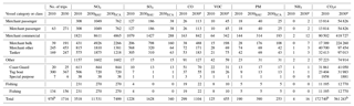
a No difference between BAU and ECA scenarios for these pollutants. b Including one (1) trip for a merchant container.
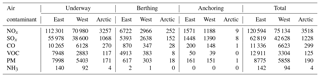
Table 22010 marine emission estimates (in tonnes) for Canada's waters by activity mode and by regions.
To project future shipping emissions in Canadian Arctic waters, a number of factors were considered. Marine traffic is expected to increase in Canada's Arctic as both current and planned resource development projects come on-line. There are several operating and planned resource development projects in Canada's north that will require regular servicing by ships, including product transport, resupply vessels, drilling ships, and platforms. In addition, it is expected that Arctic tourism, also known as ecotourism, will increase in popularity as destinations become more accessible with thinning levels of ice as a result of a changing climate, and activities of the CCG will also likely increase.
An extensive review of ship traffic projections was conducted, utilizing environmental assessment reports for resource development and other projects in the Canadian Arctic that would be serviced by ships. In addition, expected increases in other sectors, as noted above, were taken into account (Innovation Maritime and SNC-Lavalin Environment, 2013). Based on this information, a projection of the types and number of sailings of vessels and their expected emissions in the future was developed (Environment and Climate Change Canada, 2015). To validate the forecast, the growth rates were compared with published data from companies and published studies related to shipping forecasts in the Arctic (e.g., Corbett et al. 2010). In predicting future shipping traffic, a limited number of transits via the Northwest Passage were assumed, based on restricting the transit to bulk carrier vessels only and by economic viability1. Despite predictions of an ice-free Arctic by the middle to the end of this century, sea-ice variability, navigability, and dangerous weather remain constant challenges for Arctic shipping (Haas and Howell, 2015). Combined, these factors present an inherent degree of uncertainty in predicting future shipping levels in the Canadian Arctic.
Also included in Table 1 are the projected trips and emissions in Canadian Arctic water in 2030 by vessel classes. The largest anticipated increases in marine activities are from merchant vessels, particularly merchant bulk and passenger vessels. In estimating emissions related to the projected shipping activities, the emission rates were adjusted to reflect the regulatory (both domestic and international) and technological changes, such as fuel standards and fleet turnover. The MARPOL Annex VI global cap on the sulfur content of 0.5 % for fuel oil used on board ships is assumed to be in place in the BAU scenario. For the controlled scenario, it is assumed that the Canadian Arctic is designated as an emission control area (ECA) for SOx, PM, and NOx, and therefore ships are subject to comply with the 0.1 % sulfur in fuel limit, as well as the IMO Tier III NOx standards for new vessels. Under the BAU scenario, a nearly 3-fold increase in total NOx shipping emissions is expected by 2030, mostly from merchant bulk vessel activities. The increases in SOx and PM emissions (compared to the present levels) are moderate due to the global cap on sulfur content in fuel. In comparison, under the ECA scenario, the projected NOx emissions would be considerably reduced (from BAU levels) to about 2-fold of the current (2010) level in total amount, while the SOx emissions would be reduced to below the current (2010) level by the more stringent regulation in sulfur content (0.1 %).
The base model used for this study, GEM-MACH, is an on-line chemistry transport model (CTM) embedded within the ECCC numerical weather forecast model GEM (Côté et al., 1998a, b; Charron et al., 2012). A limited area version of GEM-MACH has been in use as the ECCC's operational air quality prediction model since 2009 (Moran et al., 2010). The representations of many atmospheric processes in GEM-MACH are the same as in the ECCC's AURAMS (A Unified Regional Air-quality Modelling System) off-line CTM (Gong et al., 2006), including gas-phase, aqueous-phase, heterogeneous chemistry (inorganic gas-particle partitioning); secondary organic aerosol formation; aerosol microphysics (nucleation, condensation, coagulation, activation); sedimentation of particles; and dry deposition and wet removal (in-cloud and below-cloud scavenging) of gases and particles. Specifically, the gas-phase chemistry mechanism in GEM-MACH is a modified version of the ADOM-II mechanism (Stockwell and Lurmann, 1989), with 47 gas-phase species and 114 reactions; aerosol chemical composition is represented by nine components: SO4, NO3, NH4, elemental carbon (EC), primary organic matter (POA), secondary organic matter (SOA), crustal material (CM), sea salt, and particle-bound water; aerosol particles are assumed to be internally mixed. The operational version of GEM-MACH uses a two-bin sectional representation of aerosol size distribution (Moran et al., 2010), i.e., 0–2.5 and 2.5–10 µm. The two-bin configuration was also used for this study.
In this study, model simulations were conducted over a domain with a rotated latitudinal–longitudinal grid projection at a 15 km horizontal resolution. The domain is centred over the Canadian Arctic with its southern boundary extending south of the Canada–US border (see Fig. 3). Eighty vertical, unevenly spaced, hybrid coordinate levels were used to cover between the surface and 0.1 hPa, with the lowest terrain-following model layer of about 20 m (GEM-MACH version 1.5). Several model upgrades and special considerations were made for this study:
-
Representation of sea ice and snow cover in dry deposition. Sea-ice cover from the Canadian Meteorological Centre's regional ice analysis system (Buehner et al., 2012) and snow cover and depth based on surface diagnostics were introduced to the dry deposition module to account for ice–snow cover conditions. In contrast, the base model (GEM-MACH v1.5) only takes into account permanent ice (glacier) cover in the dry deposition module. In addition, a different (lower) dry deposition velocity for O3 over snow and ice was introduced following the recommendation of Helmig et al. (2007a).
-
Chemical lateral boundary conditions. Instead of using climatology-based lateral boundary conditions as is done in the operational GEM-MACH (see Pavlovic et al., 2016), the MACC-IFS (Monitoring Atmospheric Composition and Climate, Integrated Forecast System) chemical reanalysis for 2010 (Inness et al., 2013), available every 3 h, was used to build daily chemical boundary condition files for the GEM-MACH Arctic domain. In addition, the southern boundary condition was enhanced by using the operational GEM-MACH forecast archives for the simulation time period in order to better represent the transport of pollutants from the North American continent.
-
North American wildfire emissions. Wildfire emissions were included in this study as it has been shown that northern boreal forest fires can be an important pollution source for the Arctic in summertime (Law and Stohl, 2007). Retrospective daily wildfire emissions per fire hotspot for the 2010 North American fire season were generated using the same methodology as in the ECCC's FireWork system; an air quality forecast system with representation of near-real-time biomass burning emissions (Pavlovic et al., 2016). The fire emission processing relies on the fire activity data from NASA's Moderate Resolution Imaging Spectroradiometer (MODIS) and NOAA's Advanced Very High Resolution Radiometer (NOAA-AVHRR), a fire behaviour prediction system – the Canadian Wildland Fire Information System (CWFIS; Lee et al., 2002), and the Fire Emission Production Simulator (FEPS) – a component of the BlueSky modelling framework (Larkin et al., 2009) to determine the daily total emission per fire hotspot. The per-fire-hotspot daily total emissions were then converted to hourly, chemically speciated, and grid-cell-specific emissions using the SMOKE emission processing system for use in GEM-MACH (see Pavlovic et al., 2016, for details). The fire emissions are treated as major point-source emissions in the model using the same Briggs plume rise algorithm (Briggs 1975) as anthropogenic point-source emissions, with assigned stack parameters: 3 m, 773 K, and 1 m s−1 for stack height, exit temperature, and velocity, respectively. Other fire plume injection schemes were tested in this study, including one designed using satellite-derived plume statistics. In this scheme, the vegetation-type-based (biome) statistics for plume height and depth derived from 5-year satellite observations over North America (Val Martin et al., 2010) were used to determine plume centre height and vertical spread for the flaming portion, taking into consideration atmospheric stability, while the smoldering portion of the emission is evenly spread within the modelled planetary boundary layer (PBL). The test results showed that, while the different plume injection schemes strongly impacted the modelled pollutant concentrations over the fire source region, the differences were considerably reduced at longer transport distances. As a result, the Briggs plume-rise algorithm was used in the final simulations for this study, as was used in the current FireWork system (Pavlovic et al., 2016), for distributing fire emissions.
-
Canadian marine shipping emissions. The Canadian marine shipping emission inventories described earlier in Sect. 2 were further processed into model-ready point-source emissions. The MEIT database provides ship route polygons, vessel activity information associated with each route polygon, and link-based monthly emissions by ship track, ship types, and fuel type. The database also includes stack parameters by ship type, allowing plume-rise calculations in GEM-MACH. Table 3 shows the averaged stack parameters assigned to each fuel type. To reduce data size and processing time, the more detailed ship types in the original MEIT database were aggregated, based on vessel activities, into four classes: merchant passenger, merchant commercial, fishing, and other (as indicated in Table 1). The monthly emissions for the four classes were mapped onto model grids along ship tracks, in a form of aggregated point sources (by class) and then further allocated to hourly emissions by applying uniform day-of-week and hour-of-day temporal profiles in the SMOKE emission processing system (http://www.cmascenter.org/smoke/, last access: 13 November 2018). Figure 2 shows an example of the final processed model-ready marine shipping emissions over Canadian waters used in this study: NOx emissions from shipping for the month of August both at the current 2010 and the projected 2030 (BAU) scenarios. The changes in NOx shipping emissions between the projected 2030 and current 2010 level reflect the increased shipping activities over Baffin Bay and the reduction over the Canadian east and west coast due to NA ECA regulations. For assessing the impact of shipping emissions over the Canadian Arctic waters, the shipping emissions outlined by the red line in Fig. 2 are turned on or off in the model simulations as discussed in Sect. 5.
Table 3Stack parameters for different ship emission inventories used in this study.
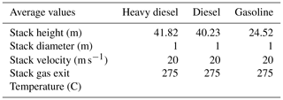
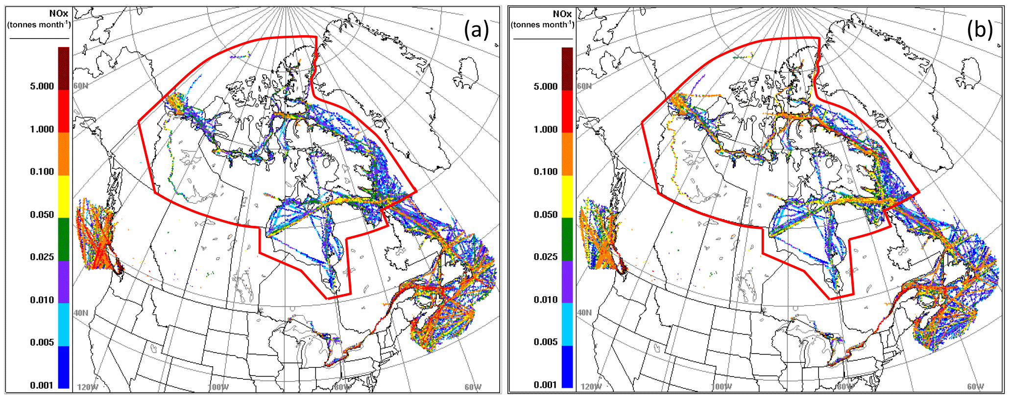
Figure 2Processed model-ready NOx marine shipping emissions for August (a) 2010 and (b) projected 2030 BAU over Canadian waters, the red line outlining the Arctic region (including Hudson Bay) which is excluded from the current North American ECA designation.
Other anthropogenic emissions included in the model simulations are based on the 2010 Canadian Air Pollutant Emission Inventory (APEI) and the 2008 US National Emission Inventory (NEI; https://www.epa.gov/air-emissions-inventories/2008-national-emissions-inventory-nei-data, last access: 13 November 2018), processed to hourly area and major point-source emissions using SMOKE. Supplementary anthropogenic emissions from the Emissions Database for Global Atmospheric Research-Hemispheric Transport of Air Pollutants (EDGAR-HTAP) v2 (see http://edgar.jrc.ec.europa.eu/htap_v2/, last access: 13 November 2018; Janssens-Maenhout et al., 2012) were used for areas outside the North American continent. Biogenic emissions were estimated on-line using the BEIS (Biogenic Emission Inventory System) v3.09 algorithms. Sea salt emissions were computed on-line within GEM-MACH based on Gong et al. (2003).
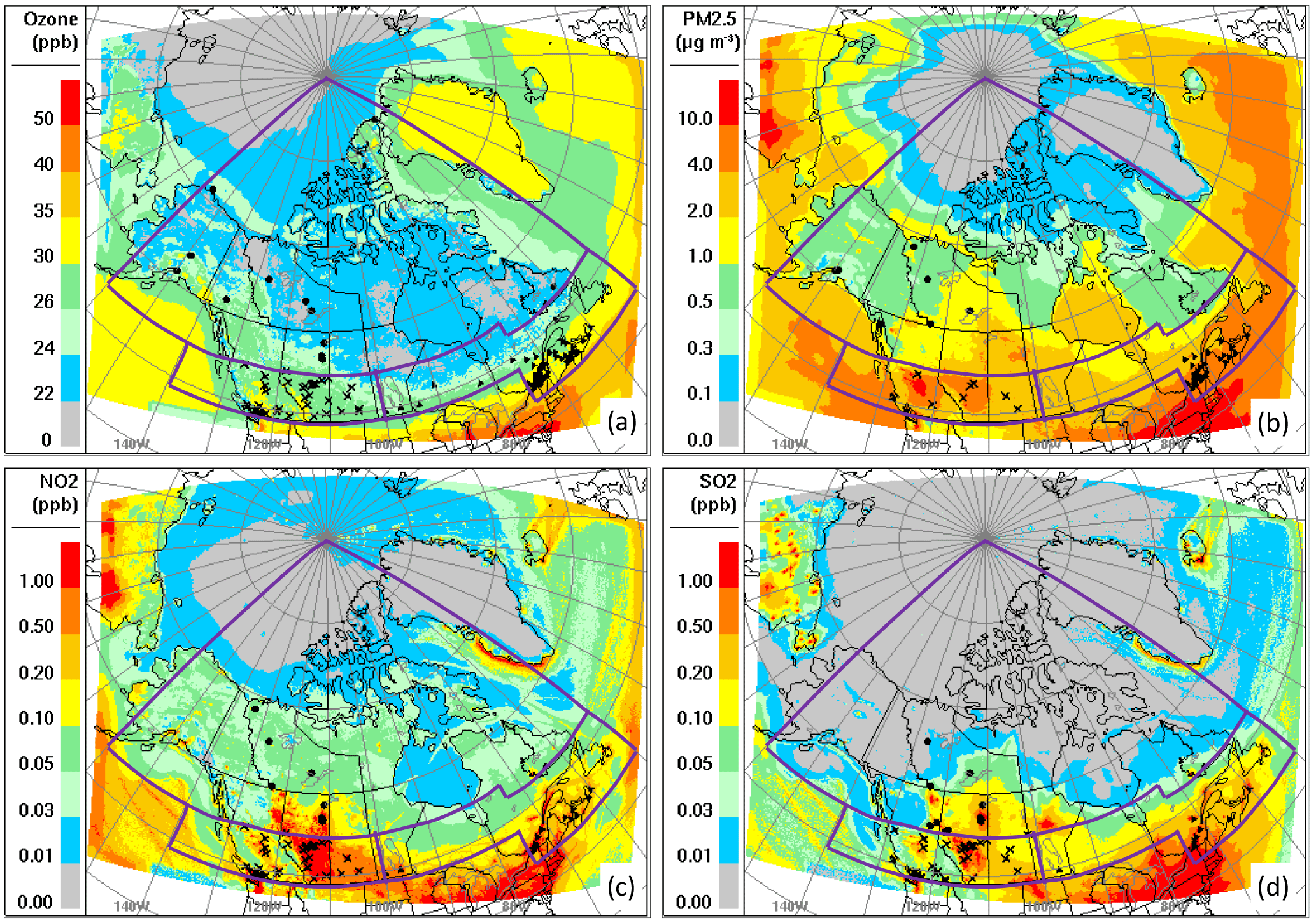
Figure 3GEM-MACH Arctic modelling domain overlaid with monitoring sites: (a) O3 monitoring sites shown on top of the modelled average ambient concentration over the July–September period; (b) the same as (a) but for PM2.5; (c) the same as (a) but for NO2; (d) the same as (a) but for SO2. (Subdivision of regions: crosses denote the sites in the western region, filled triangles denote the sites in the eastern region, and filled circles denote sites in the northern region).
The simulations were carried out for the time period of March to October 2010; the first month of the simulation is counted as spin-up and not included in the analysis. The 8-month simulation was conducted by a series of staggered 30 h runs with a 6 h (meteorology only) overlap, starting at 00:00 UTC daily, to allow meteorological spin-up from initialization; the meteorology is thus initialized at the beginning of every 30 h run using the Canadian Meteorological Centre's regional objective analyses while chemistry is continuous.
Table 4Regional evaluation for O3, PM2.5, NO2, and SO2 (hourly statistics).
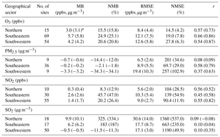
a Numbers in brackets are the scores calculated based on modelled and observed hourly time series averaged over all sites within a given region as in Im et al. (2015a, b).
The performance of GEM-MACH over the North American domain has been evaluated in a number of existing studies (e.g., Moran et al., 2011; Im et al., 2015a, b). As this is a first adaptation of the model for the Canadian Arctic domain, evaluation of model performance against available observations was carried out for criteria pollutants O3, PM2.5, NO2, and SO2, focused on the July–September period (the peak Arctic shipping season). The hourly observational data used for the evaluation were obtained from the Canadian National Atmospheric Chemistry (NAtChem; https://www.ec.gc.ca/natchem/, last access: 13 November 2018) database which contains monitoring data from the National Air Pollution Surveillance (NAPS) network in Canada (http://www.ec.gc.ca/rnspa-naps/, last access: 13 November 2018) and the US Environment Protection Agency's Air Quality System (AQS) database for US air quality data (https://aqs.epa.gov/aqsweb/documents/data_mart_welcome.html, lsat access: 13 November 2018). For O3, additional data from the World Data Centre for Greenhouse Gases (WDCGG; https://ds.data.jma.go.jp/gmd/wdcgg/, last access: 13 November 2018) were also used. Data completeness criteria of 75 % for daily data and 66 % for the full period were used to screen the data. Figure 3 indicates the monitoring sites after the data completeness screening process was completed for the 4 criteria pollutants. Overall, most of the monitoring sites within the model domain are located over southeastern Canada (Ontario, Quebec, and the Maritime provinces) and southwestern Canada (British Columbia and Alberta). There are very few sites in central Canada and north of 55∘ N. For this study, which focuses on the Canadian Arctic and northern regions, a significant challenge is the data sparsity over the region of interest: for the year 2010 (the base year for the study), Alert, on the northern tip of Ellesmere Island (82.45∘ N, 62.51∘ W), is the only air monitoring site in the entire eastern Canadian Arctic. For comparing with these ground-based monitoring observations, model results were extracted from the lowest model level (∼20 m above local surface) at given observational locations (nearest grid points). In contrast to surface meteorological observations, there is no standard height for the air chemistry measurements from the monitoring networks. However, the sampling probes are generally located between 2 and 15 m above local surface based on network guidelines. For the purpose of model evaluation, the model domain is divided into three geographical sub-regions based on general climatological and source characteristics: southwestern Canada (49–55∘ N, west of 100∘ W), southeastern Canada (49–55∘ N, 75–100∘ W and 44–53∘ N, 50–75∘ W), and the northern region (55–90∘ N, 75–160∘ W and 53–90∘ N, 50–75∘ W) covering both northern Canada and Alaska (US). The division of the sub-regions is indicated in Fig. 3.
4.1 Statistical scores
Various statistical measures were computed to evaluate model performance both at individual monitoring sites and as a group in the three geographical sub-regions. Three sets of statistics were evaluated: based on hourly averaged, daily averaged, and seasonally (July–September) averaged data. Table 4 presents the results of the hourly based, regional (sector) statistical analysis using a few selected evaluation metrics chosen to characterize overall model performance for each of the criteria pollutants, while all three sets of the statistical metrics (hourly, daily, and seasonal) are shown in the Supplement (Table S1). The statistical evaluation metrics are defined in Appendix A.
4.1.1 O3
As shown in Table 4, for ambient O3 concentrations, the model performs the best for the northern region in terms of model bias and error (e.g., MB, NMB, RMSE, and NMSE). There is an overall over-prediction of ambient O3 concentrations by ∼3 ppbv on average for the northern region, ∼4 ppbv for the southwestern region, and ∼6 ppbv for the southeastern region. The model's predictive skill increases with increased timescale as indicated by RMSE (or NMSE), with smallest errors for seasonal averaged concentrations compared to daily and hourly concentrations (Table S1). The Pearson correlation coefficient (r) for hourly O3 is highest for the southeastern region (0.66) and lowest for the southwestern region (0.54). Overall, the model showed similar skill for modelling O3 in the northern domain as the operational regional air quality models included in Im et al. (2015a) did for modelling the North America domain in terms of NMSE, RMSE, and r. Note that the statistical scores in Im et al. (2015a, b) were based on domain-mean hourly data. The equivalent statistical scores were computed for this study and shown in Table 4 (in brackets). The averaging essentially minimizes spatial variability amongst the sites within the domain (or geographical sub-regions), and hence the statistical scores on the regional averaged hourly data are much higher (in terms of RMSE, NMSE, and r) than the regional statistical scores based on hourly data at individual sites.
4.1.2 PM2.5
The regional statistical scores for PM2.5 show that the model performed best over the southeastern region, with the lowest NMB and NMSE and the highest correlation. The model under-predicted PM2.5 for the northern region, with an overall negative bias of % and poor correlation. It is worth noting, however, that there were very few sites with data available for evaluating model prediction of PM2.5 in the northern and southwestern regions, 9 in each, compared to 36 in the southeastern region. In particular, of the nine northern sites, five are located in Alaska – four in Anchorage and surrounding area, and one in Juneau, with the other four in Northwest Territories (NT). There were no PM2.5 monitoring sites available over the entire eastern Canada North region. The four sites in NT include one located in Yellowknife, the only city (and the largest community) in NT, while the others are located in smaller communities (Inuvik, Norman Wells, and Fort Liard). As PM2.5 contains both primary and secondary components, the ambient concentration at these northern sites is influenced by both long-range transport and local emissions. There are large uncertainties in both emission estimates and the spatial surrogates used for distributing estimated emissions in the northern region (note that the Canadian Emission Inventory is at provincial–territorial level). These uncertainties contribute to the poor model performance at these northern sites. For example, as shown in the Supplement, the model over-predicted PM2.5 at the Yellowknife site while under-predicting at the other NT sites (see Table S2b). Furthermore, the modelled PM2.5 at Yellowknife site is dominated by “crustal material” (see Fig. S1 in the Supplement), which is a major component of primary PM emissions in NT. The spatial surrogates used for crustal material are paved roads and mine locations. The paved road network in NT used in processing the 2010 emission inventory was very limited, mainly concentrated in Yellowknife and its surroundings. As for mine locations, the surrogate was based on place-of-work data from the 2006 Canadian Census for the mining industry (http://www12.statcan.ca/census-recensement/2006/rt-td/pow-ltd-eng.cfm, last access: 13 November 2018), which can lead to allocating mining-related emissions to cities rather than actual mining operation sites, as many mining company employees work at headquarters which tend to be located in cities (e.g., Moran et al., 2015). For the Inuvik site on the east channel of the Mackenzie Delta, the model under-prediction may be partially attributable to an underestimation of emissions from the oil fields in Prudhoe Bay on Alaska's North Slope in the US 2008 Emission Inventory (https://www.epa.gov/air-emissions-modeling/20072008-version-5-air-emissions-modeling-platforms, last access: 13 November 2018).
4.1.3 NO2
For predicting NO2, the model performed the best, overall, for the northern sites with the lowest NMB (8.3 %) and RMSE (5.6 ppb) and highest r (0.56), based on hourly data (Table 4). However, the relatively small overall bias may be misleading, as there are large positive and negative model biases at the individual northern sites (Table S2c in the Supplement). This is indicated by the large NMSE value (104 %). The 10 northern sites here include 4 in NT, where the model generally under-predicted, and 6 in the lower Athabasca oil sands region in Alberta, where the site-specific model biases, in terms of NMB, varied between −64 % (at Fort Chipewyan) and 143 % (at Syncrude UE1), indicating significant heterogeneity. Again the model performance at these sites is influenced by the uncertainties (challenges) in estimating and representing emissions in these regions of Canada (ECCC & AEP, 2016; Zhang, et al., 2018). Also note that the NO2 observations from the NAPS network were reported in an increment of 1 ppb, which will have a considerable impact on the statistical scores, particularly at more remote sites where NO2 concentrations are low and of the order of < 1 ppbv. The high correlation between the modelled and observed seasonal averaged concentrations (Table S1) indicates, however, that the model captured the geographical distribution of the regional NOx sources and plumes reasonably well.
4.1.4 SO2
The statistical scores for model prediction of SO2 are considerably poorer than those for the other criteria pollutants discussed above, with large biases (in terms of NMB) and errors (in terms of NMSE). Note that the reference unit for SO2 in this comparison is µg m−3 at standard atmosphere (0 ∘C) because the reported SO2 concentrations were converted to this unit in the NAtChem database. There are several factors to be considered when interpreting these statistical scores. Firstly, the group statistical scores for the northern sites are largely influenced by the sites located in the lower Athabasca oil sands region in Alberta and the Peace region of northeastern British Columbia (see Table S2d), with considerable oil and gas industries there. The monitoring sties in these regions are located at or near industrial facilities. The modelled SO2 at these locations are primarily driven by the model emission inputs. There are large model biases at these locations, again indicating potential deficiencies in emission estimates and processing in these regions (e.g., spatial and temporal allocation of the annual emissions; e.g., ECCC & AEP, 2016; Gordon et al., 2017; Zhang et al., 2018). Secondly, similar to the case of NO2 discussed above, there is also a precision issue with monitoring data reporting: SO2 concentrations are reported at 1 ppb (or ∼2.86 µg m−3) increments. This is particularly problematic for model evaluation at more remote sites (such as those in the Northwest Territories), where SO2 concentrations are generally below 1 or 2 ppb, and the reported concentration values toggle between 0, 1, and 2 ppb (or 0, 2.86, and 5.72 µg m−3 after conversion in the NAtChem database). Again, despite the large mean bias (∼10 µg m−3) and RMSE (seasonal, ∼16 µg m−3), the correlation between the modelled and observed seasonal averaged SO2 concentrations in the northern region is high (r=0.90; see Table S1), indicating that the model was able to capture the spatial distribution and structure of the observed concentrations.
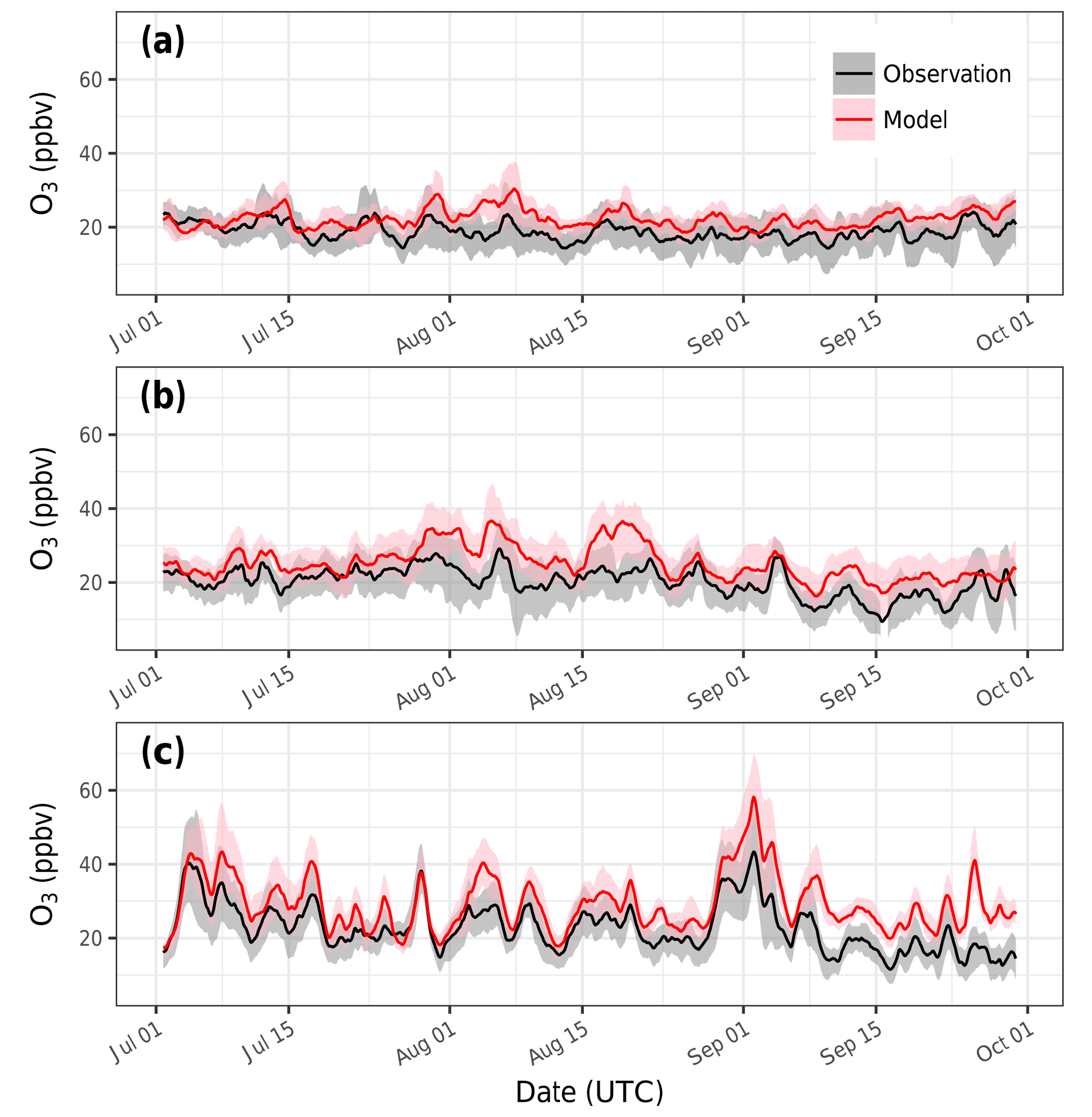
Figure 4Regional averaged O3 time series (24 h running mean), modelled and observed: (a) northern, (b) southwestern, (c) southeastern; shades indicate 1st–3rd quartile range.
4.2 Time series
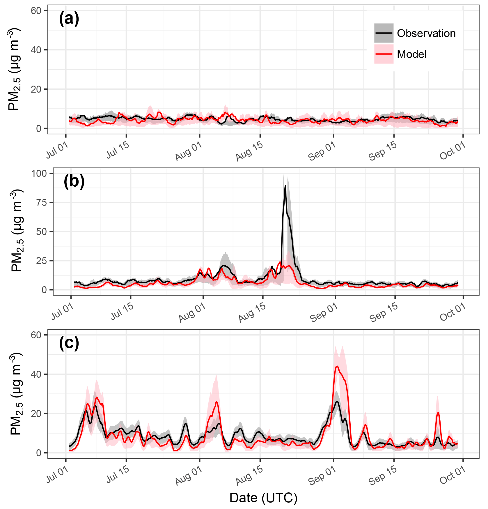
In addition to the statistical scores, the model's ability of simulating the temporal variations in ambient concentrations of criteria pollutants during the Arctic shipping season is examined here. Figures 4–7 show the model–observation comparison of the regional averaged time series (shown as 24 h running means) of O3, PM2.5, NO2, and SO2 for the three sub-regions. Given the monitoring site locations, the “northern” regional average really represents only northwestern Canada (and Alaska in the case of O3 and PM2.5).
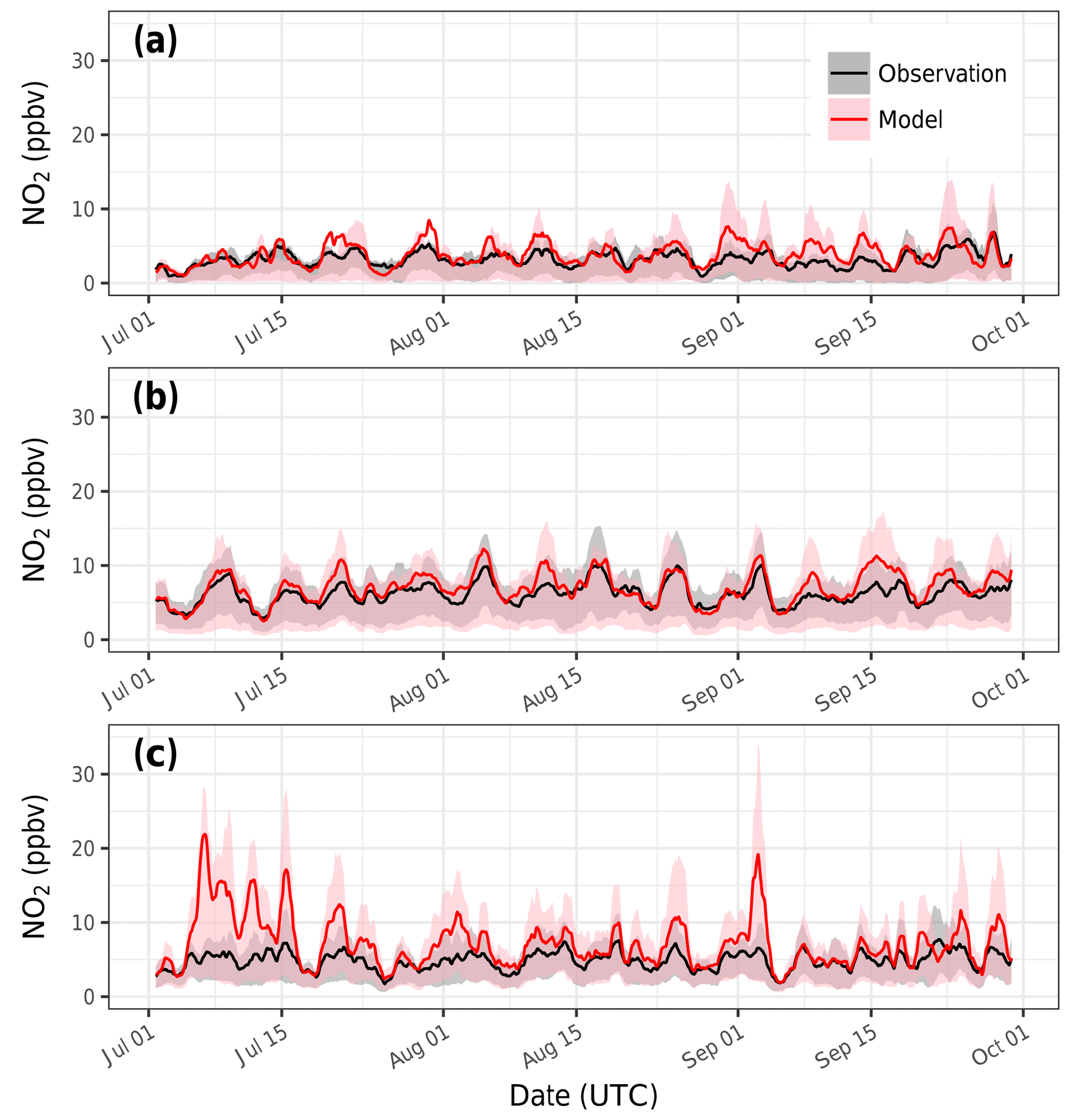
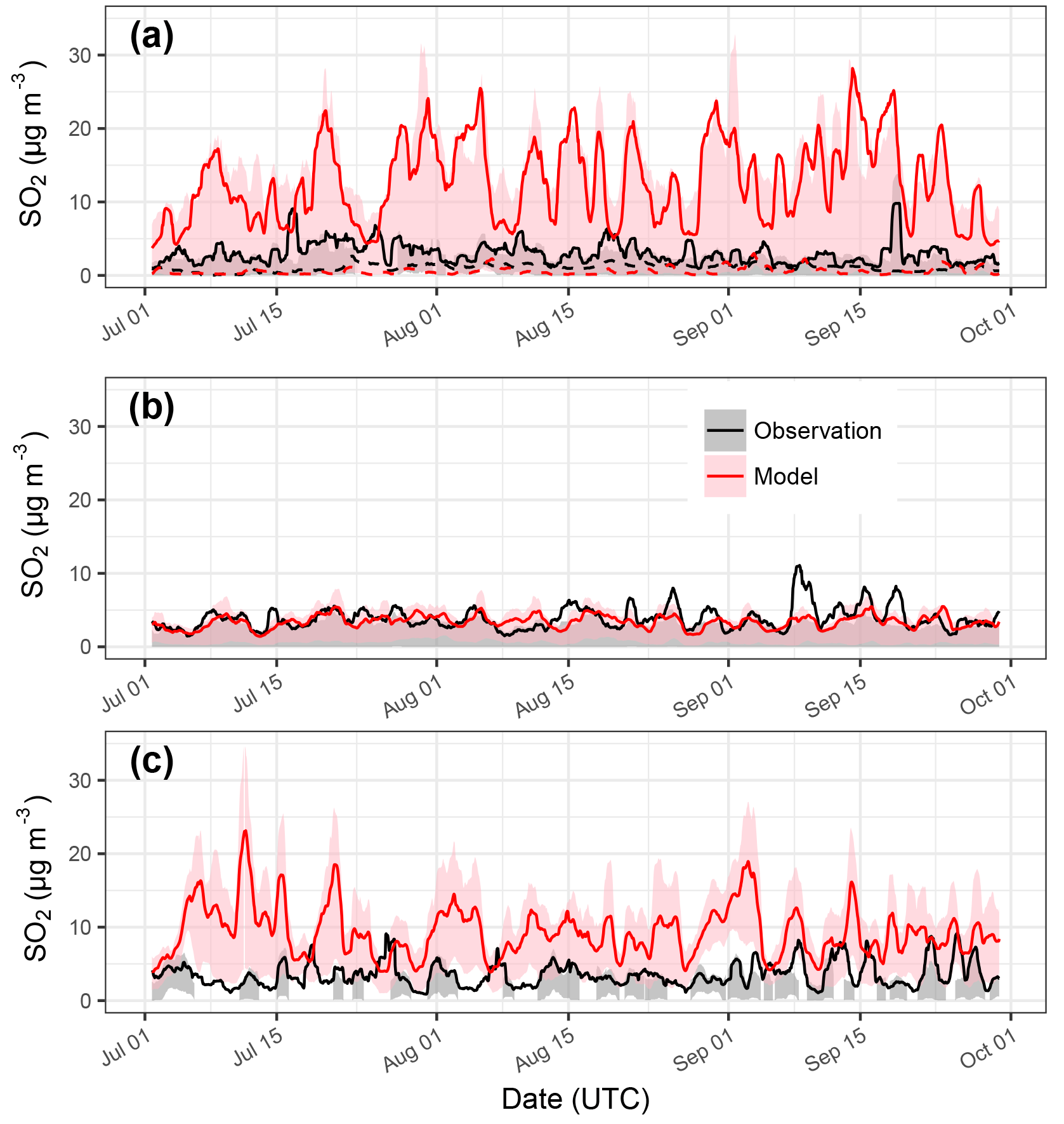
Figure 7Same as Fig. 4 but for SO2. Dashed lines in (a) denote time series excluding sites in the Athabasca oil sands and northeastern BC oil and gas industry areas (see text).
The regional O3 time series show that the overall temporal variability is smallest at the northern sites and greatest at the southeastern sites most strongly influenced by regional and synoptic events. The model generally captured the temporal variations well. A positive bias in model prediction is evident. For the southwestern region, the overall positive bias was largely contributed by the over-prediction of the O3 nighttime minima (not shown). The nighttime model bias can be a result of the model's difficulty in simulating (or resolving) the stable nocturnal boundary layer, where small differences in the actual O3 sources and/or sinks, like O3 dry deposition, can have a large impact on O3 concentration gradients, which might also be reflected in significant differences in observed and simulated nocturnal O3 for different reference heights. The more pronounced over-prediction events during the month of August at the northern and southwestern sites are likely associated with large wild fire events in British Columbia during that period. The model tends to over-predict O3 in fire plumes (Gong et al., 2016; Pavlovic et al., 2016), particularly within a short transport time. A number of factors may be contributing to the over-prediction, including uncertainties in emission factors and the lack of representation of aerosol shading in the model, which may lead to an overestimation of photolysis rates in fire plumes. The possible causes are currently under investigation.
The northern regional averaged PM2.5 time series during the July–September period is dominated by variations at small scales, implying a strong influence of primary components from local sources at these northern sites, while the southeastern regional PM2.5 time series is more controlled by variations at larger scales, or regional events, implying the dominance of secondary components and/or regional sources. The southwestern time series contains the signature of both local and regional influences with the main regional events in August, coinciding with the major wild fire events in BC at that time. The model captured the general trends well particularly for the regional events, while it had difficulty tracking the local-scale variations, which is not unexpected given the model resolution.
The regional averaged NO2 time series shows a nearly 7-day cycle, particularly for the southwestern and northern sites. The model predictions compare well for the northern and southwestern regions. For the southeastern region the model captured the general trend well, but there is a tendency for more significant over-prediction, particularly at the beginning of July. Significant over-predictions of NO2 over eastern Canada during this time period from the operational GEM-MACH forecast were also shown in the evaluation of Moran et al. (2011). It should be noted that the southeastern sites in this study are in close proximity to the southern boundary and are more likely to be influenced by the model southern boundary condition, which comes from the operational GEM-MACH forecast archives.
As a reflection of the SO2 regional statistical scores discussed above, the comparison of regional averaged time series of the observed and modelled SO2 for the northern region is strongly influenced by the sites located near oil and gas facilities. Also shown in Fig. 7a are the regional averaged time series, excluding the sites in the Athabasca oil sands and northeastern BC oil and gas industry areas (in dashed lines). It is evident that these sites are skewing the regional averages. The large discrepancies between the model simulation and observations at these sites are indicative of the possible deficiencies in the existing emission inventory and the emission processing for these facilities. The model and observations are in much better agreement at the northern sites, away from the oil and gas facilities. The model simulation also compares well with the observations in the southwestern region, closely tracking the observed general trend at the regional scale. The comparison for the southeastern region shows a general over-prediction by the model. In particular, the modelled group-averaged time series shows a higher regional baseline level than indicated by the observations. As shown in Fig. 3d, these southeastern sites are situated under the influence of the model's southern boundary, and the modelled average SO2 concentration over the July–August–September period shows a regional plume originating from the southern boundary, reflecting the influence of a major SO2 source area in the Ohio River valley. Note that the emission inputs used by the operational GEM-MACH forecast in 2010, the basis for the model southern chemical boundary condition for the current study, were based on the 2006 Canadian, 2005 US, and 1999 Mexican national emission inventories (Moran et al., 2011). Due to the various US EPA emission control programs in recent years (e.g., Acid Rain Program, NOx Budget Trading Program, Clean Air Interstate Rule; see https://www.epa.gov/airmarkets, last access: 13 November 2018), SO2 (and NOx) emissions over eastern US have reduced considerably between 2005 and 2010. The model over-prediction of ambient SO2 (and NO2, see above) in the southeastern region in this study can therefore be, at least in part, attributed to the possible over-prediction of SO2 (and NO2) from the operational GEM-MACH over the US northeast.
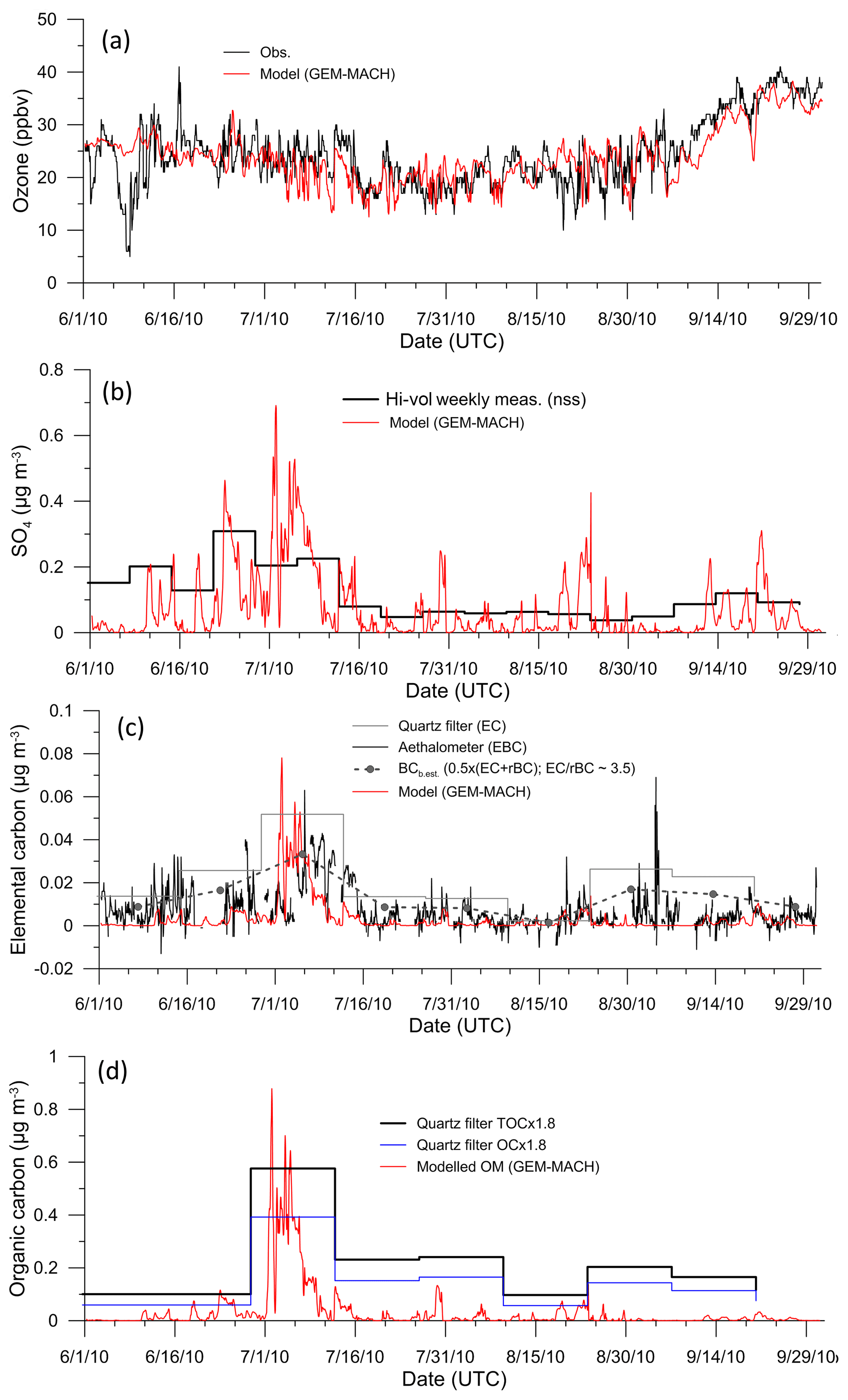
Figure 8Comparison with observations at the Alert site for June–September 2010: (a) O3, (b) sulfate; nss denotes non-sea-salt, (c) EC, and (d) OC (OM).
Canadian high Arctic site, Alert
Several long-term monitoring measurements of atmospheric constituents have been carried out at ECCC's Alert baseline observatory located at the northern tip of the Ellesmere Island (82.45∘ N, 62.51∘ W) – one of the Global Atmosphere Watch global network stations. For the year 2010 the measurements included, in addition to O3 (continuous, hourly), inorganic aerosol components from weekly high-volume samplers (Sirois and Barrie, 1999; Sharma et al., 2004), OC and EC using a thermal method from biweekly quartz filter samples (Huang et al., 2006), and equivalent black carbon (EBC) from aerosol light absorption measurements using an aethalometer (Shama et al., 2017). These data are all used for evaluating model prediction at this high Arctic location. The comparisons of the modelled and observed time series of O3, sulfate, EC, and OC (OM – organic matter) over the June–September period are shown in Fig. 8.
The model is seen to predict O3 very well at this high Arctic site; the modelled O3 time series tracks closely with the observations, reaching a minimum at the end of July and the beginning of August and then rising steadily throughout late August and September. The model did not predict the low ozone event observed at the beginning of June. The low ozone event may be the result of ozone depletion involving bromine chemistry within the Arctic marine boundary layer (Barrie and Platt, 1997), which is not represented in this version of the model. The modelled sulfate also compared well, particularly in terms of the general trend and magnitudes, with the non-sea-salt sulfate measurements based on weekly samples.
The modelled EC is compared with both EBC derived from the continuous aethalometer measurement and EC measurement using a thermal desorption method from quartz filter sampling (biweekly in 2010). It can be seen that while the modelled EC is overall biased low compared to the EBC from the aethalometer measurement, and biased lower still compared to the biweekly EC measurement, the model captured the general trends shown in both observation sets. In particular, the event in early July was captured by the model well, which is attributable to biomass burning emissions from northern Canada. Sharma et al. (2017) discussed in depth the various techniques for measuring black carbon mass at the Alert observatory and showed that EC mass based on the thermal method is highest over summer months, followed by the EBC mass estimate from the aethalometer measurement; both are significantly greater than the refractory BC (rBC) mass measurement using the Single Particle Soot Photometer (SP2). As a best estimate of BC mass at Alert for comparison with chemical transport models, Sharma et al. (2017) recommended using a combination of EC and rBC or EC with a scaling factor of , where α is the EC ∕ rBC ratio. The scaled EC (using α of 3.5, based on Sharma et al., 2017) is indicated in Fig. 8c with solid dots connected by the dashed line. However, one needs to be careful in comparing the modelled aerosol EC component with BC measurements, as they may not be strictly comparable depending on the measurement techniques (e.g., Petzold et al., 2013; Sharma et al., 2017) and how EC (or BC) is modelled (including emission input).
The modelled organic aerosol component (POA + SOA) is compared with the biweekly measurement of OC from the thermal desorption method. For this comparison the measured OC is converted to OM by applying an OM ∕ OC ratio of 1.8. The total OC (TOC) from the OC ∕ EC analysis includes OC released at 550 ∘C and pyrolyzed OC (POC) plus inorganic carbonate carbon (CC) released at 850 ∘C. The estimate of CC fraction of POC + CC is 40 % at Alert in summer time. The CC fraction was removed from the TOC measurement for the comparison in Fig. 8d based on the CC ∕ (POC + CC) fraction. The measured OC component (at 550 ∘C) is also shown in Fig. 8d, indicating that this is the dominant component of measured TOC at this site. Overall the model under-predicted the organic aerosol component at this site compared to the measurement based on the OC ∕ EC analysis but again captured the event in the beginning of July (as in the case of EC comparison above) associated with long-range transport of biomass burning pollutants. Recent observations conducted in the Canadian Arctic have suggested possible marine secondary organic aerosol production over the Arctic Ocean during summer time from oceanic and biological sources (e.g., Willis et al., 2016), which may explain at least in part the model under-prediction of organic aerosols (Gong et al., 2017).
The evaluation results presented in this section demonstrate that GEM-MACH's skill in predicting ambient O3 and PM2.5 in the Canadian northern and Arctic regions is comparable to the skill level of the current operational air quality forecast models in North America and Europe. The model has reasonable skill in predicting NO2 and SO2 in the north at a regional scale; at local scales the model prediction is strongly influenced by emission inputs. The evaluation indicates a deficiency in representing local emissions in the remote north and the need for improved emission estimates and representation for the oil and gas facilities in northeastern British Columbia and the Athabasca oil sand region in northern Alberta. There is also a significant data gap in northern Canada, particularly the eastern Arctic, for air quality monitoring and for model evaluation. The model, however, is able to simulate the observed ambient O3, and some of the PM components at Alert well, the only air quality monitoring site in the eastern high Arctic.
While there has not been many regional modelling studies focused on the Arctic and northern regions, there are some existing studies mostly using global models with a focus on the Arctic. For example, Emmons et al. (2015) reported a multi-model intercomparison project where model simulations using a number of models (nine global and two regional) were compared with observations conducted during the 2008 International Polar Year in the Arctic. In particular, comparisons were made with aircraft measurements conducted in northern Canada and into the Arctic over a 12-day period during late June to early July. They found that models generally under-predicted O3 and SO2 in the mid-troposphere and over-predicted NO2 in the boundary layer during this summer period. A direct comparison in terms of model performance to the current study is difficult to make, as the model evaluation in the current study is based on surface observations over a longer time period. Shindell et al. (2008) also compared global model simulations, conducted under the Task Force on Hemispheric Transport of Air Pollution (TF HTAP), against long-term observations at selected Arctic sites including Alert and Barrow. They found that the models generally under-predict O3 at Barrow during summer by as much as 10 ppb, and that models performed poorly in predicting sulfate and BC at Alert. In comparison, the model evaluation from the current study demonstrates much better model skills in predicting the ambient concentrations of these pollutants in the Arctic (e.g., comparisons shown in Fig. 8).
The model evaluation conducted in this study is mainly focused on the atmospheric chemistry aspect. However, the model's ability to simulate the vertical structure and stability of the coastal marine boundary layer has an important influence on assessing the shipping emission impact on ambient concentrations. Although the operational performance of the meteorological model GEM (the hosting model for GEM-MACH) has continuously been evaluated against surface and upper air observations and compared against other NWP models of leading operational forecasting centres in the world, the Arctic region alone had not been given significant attention in the past operational evaluation exercises. To evaluate the GEM-MACH performance in simulating the Arctic marine boundary layer, we compared the modelled vertical temperature profiles with upper air soundings at a number of coastal sites in the Arctic along the main shipping channels for the month of July in 2010. On average, the modelled vertical temperature profiles compare with the observations well (see Supplementary Materials, Fig. S2a). We also attempted to diagnose boundary-layer (BL) heights based on the bulk Richardson number, following Mahrt (1981) and Aliabadi et al. (2016a), from both modelled and observed profiles at these selected Arctic sites. On average, the model and observation diagnosed BL heights are within ±30 % of each other (see Fig. S2b). Particularly, for the Resolute site, the model and observation diagnosed BL heights for July, averaged at 315.4 m and 267.4 m, respectively, are comparable to the estimated BL heights, 274±164 m, over the same area during a recent field campaign in July 2014 (Aliabadi et al., 2016b). It should be pointed out, however, that there is a large ambiguity in the definition of BL height under stable conditions (such as the case of the Arctic marine BL), and the diagnosed BL height can vary considerably depending on the particular method (or parameterization) used (e.g., Aliabadi et al., 2016a). A more detailed examination of GEM's forecast capability in the Arctic is being pursued under the Year of Polar Prediction (YOPP) initiative (https://public.wmo.int/en/projects/polar-prediction, last access: 13 November 2018).
The impact of shipping emissions in the Canadian Arctic is assessed by comparing pairs of model simulations, with and without the Canadian portion of the Arctic shipping emissions, under three scenarios: current (2010), projected 2030 BAU, and 2030 with ECA (see Sect. 2 above). To isolate the impact of shipping emissions, only shipping emissions were changed between the different scenarios, while meteorology, land use, and other emissions (such as non-shipping anthropogenic emissions and wild fire emissions) remained the same for all scenario simulations. The analysis is focused on the July–August–September (JAS) peak Arctic shipping period. It should also be stated that the impact is mostly assessed in relative terms in this study for these considerations. (1) Since the modelled future scenarios do not reflect changes in forcing factors other than shipping emissions, it is more meaningful to assess the modelled relative response to the emission changes. (2) There is robustness in using a model to assess relative changes: past studies involving multi-models have shown that, despite the large difference in performance amongst models, only relatively minor differences were found in the relative response of concentrations to emission changes (Jones et al., 2005; Hogrefe et al., 2008).
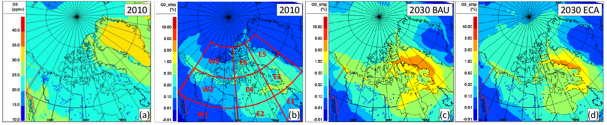
Figure 9Modelled mean ambient O3 concentrations for July–August–September (shipping season) of 2010 base year (a), and relative contribution from Canadian Arctic shipping emissions for the 2010 base year (b), 2030 BAU (c), and 2030 ECA (d). (The geographical subdivisions indicated on (b) are referred to in the statistical assessment).
5.1 On ambient air concentration of criteria pollutants
The modelled JAS-averaged ambient concentrations of O3, PM2.5, NO2, and SO2, and the corresponding contributions from Arctic shipping are shown in Figs. 9–12, with a focus on the Canadian northern and Arctic regions. The percentage ship contributions shown were computed as
where i and j denote pollutants (e.g., O3, PM2.5, NO2, and SO2) and scenarios (i.e., 2010 base case, 2030 BAU, and 2030 ECA), respectively.
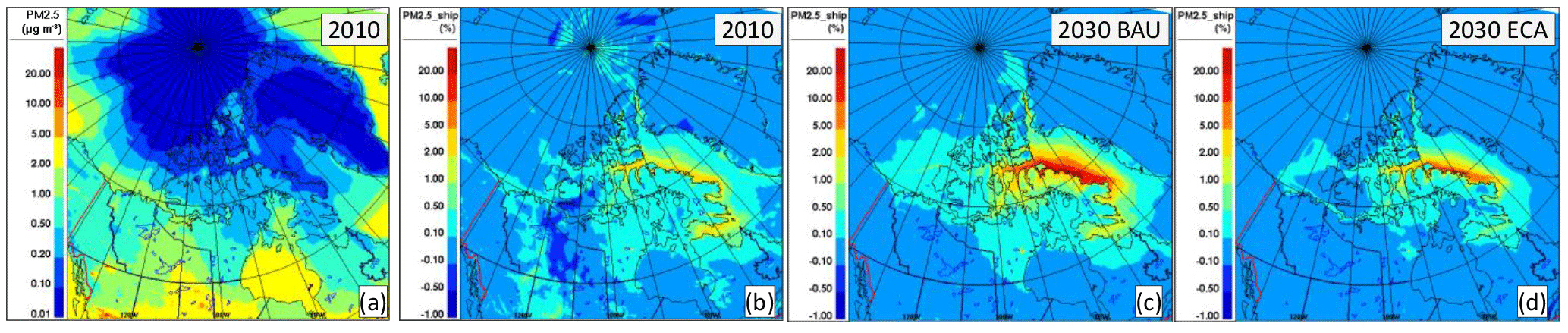
Figure 10Modelled mean ambient PM2.5 concentrations for July–August–September (shipping season) of 2010 base year (a), and relative contribution from Canadian Arctic shipping emissions for the 2010 base year (b), 2030 BAU (c), and 2030 ECA (d).
The modelled ambient O3 concentrations averaged for the JAS period range between 20 and 25 ppbv over most of the eastern Arctic (Fig. 9a). The relatively high ambient concentrations over Greenland are due to the high elevation. The Arctic shipping emissions contribute to less than 1 % of the JAS-averaged O3 concentration at the present level (or 2010 base case); the impact is mostly felt between 50∘ and 100∘ W (Fig. 9b) and Mackenzie Bay in the west. At the projected 2030 BAU level, the model predicted considerably greater shipping contributions, showing up to 5 % of the JAS-averaged ambient O3 concentration (Fig. 9c); the area where shipping emissions contribute greater than 0.5 % extends to almost all of the eastern Canadian Arctic (or Nunavut territories, NU). This is in response to the projected increase in NOx emissions from Arctic shipping in the 2030 BAU scenario. For the 2030 ECA scenario, the model predicted shipping contributions to O3 concentrations are reduced compared to the 2030 BAU scenario but are still greater than the present 2010 base-case level (Fig. 9d), particularly along Davis Strait and Baffin Bay. This is consistent with the fact that projected NOx emissions from Arctic shipping in 2030 under ECA are intermediate between current 2010 and 2030 BAU levels (see Table 1).

Figure 11Modelled mean ambient NO2 concentrations for July–August–September (shipping season) of 2010 base year (a), and relative contribution from Canadian Arctic shipping emissions for the 2010 base year (b), 2030 BAU (c), and 2030 ECA (d).
The modelled JAS-averaged ambient PM2.5 concentrations show a general south-to-north decreasing gradient, from a few micrograms per cubic metre in the sub-Arctic regions to below 0.1 µg m−3 in the high Arctic (Fig. 10a). As PM2.5 consists of both primary and secondary components, the impact of shipping emissions accentuates the shipping channels (Fig. 10b–d) more than in the case for O3. The contributions from Arctic shipping emissions to the JAS-averaged PM2.5 concentrations are in the range of 1 %–5 % along the eastern Parry Channel, Pond Inlet, and north of Baffin Island and generally < 0.5 % over land at the present level (2010 base case; Fig. 10b). At the projected 2030 BAU level, the contributions from Arctic shipping emissions to ambient PM2.5 concentrations are predicted to increase to 5 %–20 % over the main shipping channels, particularly along the east coast of Baffin Island and Lancaster Sound area (Fig. 10c). The greater contribution in this case is due to the projected increase in both primary PM emissions and PM precursor emissions (of SO2, NOx, and VOCs) from shipping; this is evident from examining the shipping contributions to individual PM components. The components contributing to the increase in total PM due to shipping include primary PM, such as elemental carbon, primary organics, and crustal material and secondary PM, such as sulfate, ammonium, and nitrate, (see Figs. S3–S8 in the Supplement). Again, for the 2030 ECA scenario, the model predicted a considerably reduced contribution from shipping in comparison with the 2030 BAU scenario (Fig. 10d), primarily resulting from the drastic reduction in sulfur emissions if ECA is in effect over the Arctic waters.

Figure 12Modelled mean ambient SO2 concentrations for July–August–September (shipping season) of 2010 base year (a), and relative contribution from Canadian Arctic shipping emissions for the 2010 base year (a), 2030 BAU (c), and 2030 ECA (d).
For NO2 and SO2, both primary pollutants, the model shows that Arctic shipping emissions make major contributions to ambient concentrations over and near the Arctic waterways. The modelled JAS-averaged ambient concentrations of NO2 and SO2 are 0.02–0.1 and 0.001–0.01 ppbv, respectively, over the eastern low Arctic and sub-Arctic, and generally below 0.02 ppbv and 0.001 ppbv, respectively, over the high Arctic (Figs. 11a and 12a). The relatively elevated concentrations around the lower east coast of Greenland primarily reflect shipping emissions based on the 2010 HTAP inventory (used in this study for areas outside North America, see section 3 above). At current (2010) levels, based on the model simulations, the Arctic shipping emissions contribute to 10 %–50 % (Fig. 11b) and 20 %–100 % (Fig. 12b) of the ambient NO2 and SO2 concentrations, respectively, over the Arctic shipping channels. The contributions are greatly increased at the projected 2030 BAU level, in the case of NO2, to > 50 % over most of the shipping channels (Fig. 11c) in response to a nearly 3-fold increase in NOx emissions from Arctic shipping. In contrast, the contributions from Arctic shipping to ambient SO2 concentrations are only moderately higher at the projected 2030 BAU level compared to the present 2010 level (Fig. 12c vs. 12b). This is in response to a more moderate (∼32 %) increase in SO2 emissions over the 2010 level (assuming the global cap of 0.5 % on sulfur content in fuels used onboard ships is in effect, i.e., MARPOL Annex VI Regulation 14.8). Under the 2030 ECA scenario, there is a moderate decrease in the Arctic shipping contribution to ambient NOx concentration (Fig. 11d vs. 11c), while there is a drastic decrease in the Arctic shipping contribution to the ambient SO2 concentration (Fig. 12d vs. 12c). This is in accordance with the reductions of 35 % and 79 % in NOx and SO2 emissions, respectively, from the 2030 BAU level when assuming the NA ECA controls are in effect over the Canadian Arctic waters. In fact, the ECA control on sulfur emissions would bring down the shipping contribution to the ambient SO2 concentration to below the current 2010 base-case level.
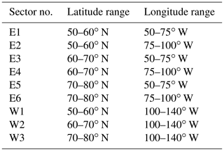
Table 5Division of geographical sectors over the Canadian Arctic and northern regions for the assessment.
5.1.1 Statistical assessment by geographical sectors
A more quantified (and area-specific) assessment of the impact of ship emissions was carried out by dividing the area of interest into nine geographical sectors (see Table 5; also indicated in Fig. 9b), and shipping contribution statistics were computed for each of the geographical sectors. Table 6 summarizes the mean, median, and maximum percentage contributions from Arctic shipping emissions to the JAS-averaged ambient concentrations of criteria pollutants for each of the nine sectors. The percentage contributions (as defined in Eq. 1) were evaluated at individual grid points, and statistics were then computed over all grid points within a given geographical sector. Generally speaking, the shipping impact is greater over the eastern Canadian Arctic than the western Canadian Arctic, due to the proximity of the area to the Arctic shipping channels. In addition, the western region of the Canadian Arctic is more strongly impacted by North American boreal forest fire plumes during the summer season, with relatively higher background concentrations of these criteria pollutants than in the eastern region (e.g., Gong et al., 2016).
Table 6Percentage contribution from Arctic shipping to ambient concentrations of criteria pollutants, by geographical sectors (see Table 1), for the July–August–September period.
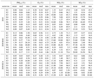
At the current level (2010), the contribution statistics for O3 show that both mean and median percentage contributions from Arctic shipping are relatively uniform over the eastern sectors, with slightly higher contributions over sectors E3 and E4 at around 0.3 % and the rest of the eastern sectors at around 0.2 %. As for PM2.5, the shipping contributions are higher over the northeastern sectors (north of 60∘ N) and highest (> 0.5 % in mean value) over sectors E3 and E6, both of which are in close proximity to the Arctic shipping routes (see Fig. 1). Shipping contributions to ambient concentrations of NO2 and SO2 are much higher in comparison to O3 and PM2.5 and are again highest over sectors E3 and E6 (with mean percentage contributions: > 10 % for NO2 and ∼20 % and higher for SO2). Shipping contributions over E4 (in close proximity to ship traffic over Hudson Bay) and W6 (in close proximity to the Beaufort Sea) are also pronounced in this case. Sector E6 has the highest relative contribution from Arctic shipping emissions, which is attributed to its proximity to northern Arctic shipping routes and it being the most remote region with the lowest background concentrations, and hence, the most sensitive area to local emissions. Note that the statistics shown in Table 6 imply that the probability distribution functions (PDFs) of the percentage shipping contributions for pollutants PM2.5, NO2, and SO2 are highly skewed (i.e., large differences between means and medians and confirmed by further statistical analyses undertaken but not shown here), while the percentage contributions for O3 are relatively normally distributed (i.e., small differences between mean and median values). This is consistent with O3 being a secondary pollutant, and, with its relatively long atmospheric lifetime, O3 has much higher background ambient concentrations (and hence a smaller relative contribution from shipping emissions) compared to the other pollutants assessed in this study.
At the projected 2030 BAU level, there is an overall increase in the shipping contributions to ambient concentrations of the criteria pollutants over all sectors (with the exception of sector W1, which is far away from Arctic shipping routes). The average contribution from shipping to ambient O3 concentrations increases to about 1 % or higher over the northeastern sectors (from < 0.4 % currently). The average shipping contribution to the ambient PM2.5 concentration increases more significantly over sectors E3, E5, and E6, e.g., 2 % over E3 compared to 0.6 % at the current level. The most significant contribution of ship emissions to ambient levels of pollutants is for NO2, for which average contributions are over 30 % in sector E6 and reaching 20 % in sector W3. The increase in shipping contribution to ambient SO2 concentrations at the projected 2030 BAU level is overall predicted to be more moderate compared to the case of NO2 for most of the sectors, except for sector W3, where the average shipping contributions increase to nearly 30 % from just over 10 % at the current level. As mentioned above, for SO2, the projected increase in shipping activity is partly offset by the global sulfur cap coming into effect in 2020 (or by 2025 with a 5-year delay, i.e., MARPOL Annex VI Regulation 14.8). If the same North American ECA regulations were to be applied within the Arctic waters in 2030 (i.e., with 0.1 % sulfur cap and the IMO Tier III NOx standard for new vessels, the 2030 ECA scenario), the shipping contribution to ambient SO2 concentrations would be well below the current (2010) level, and the shipping contribution to ambient PM2.5 would be brought roughly back to the current level. There would be reductions in shipping contributions to the ambient NO2 and O3 concentrations compared to the 2030 BAU scenario, but the contributions would still be greater than the current level. This is in line with the less stringent regulation (in comparison to sulfur) on NOx under the NA ECA.
5.1.2 Population-weighted concentrations
Since criteria pollutants are closely related to health effects, it is pertinent to look at the impact of Arctic shipping emissions in terms of population-weighted concentrations. Population-weighted concentrations are often used in population exposure and health effect analyses (e.g., Ivy et al., 2008, Mahmud et al., 2012). It is calculated as
where i designates each computational grid cell, and popi and conci denote population and concentration, respectively, at grid cell i. Here population-weighted concentrations of the criteria pollutants are calculated for Canada's eastern and western Arctic, defined as north of 60∘ N, 60–100∘ W and 100–140∘ W, respectively.
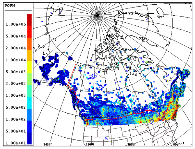
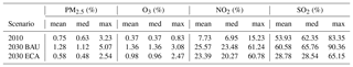
Figure 13 shows the gridded population density over the model domain based on the 2010 US and 2011 Canadian population data. As shown, over the eastern Arctic, the populations are mostly distributed along coastlines in small isolated communities and are thus more directly subjected to the impact from shipping emissions than over the western Arctic. The time series of the population-weighted concentrations of O3, PM2.5, NO2, and SO2 and the corresponding shipping contributions over the June–September period are plotted in Fig. 14a–d. Overall the population-weighted concentrations are higher in the western Canadian Arctic than in the east. The communities and population centres are larger in the west and, in addition, the western Arctic is more affected by North American boreal forest fire emissions in the summer months (e.g., Alaska, northern British Columbia, and northern prairies; Gong et al., 2016). Conversely, the relative contributions from ship emissions are higher in the east than in the west, due to the proximity of the eastern communities to the shipping channels and cleaner background air. The population-weighted O3 concentration over the eastern Arctic shows an overall summer minimum in July and a slow recovery during late summer and early fall, which is consistent with the general O3 seasonal trend observed at the Arctic sites (Helmig et al., 2007b). In contrast, the time series for the western Arctic shows higher values in mid-July and early August, likely due to biomass burning impact in the region. The shipping contribution is relatively uniform over the peak shipping season (JAS) over the eastern Arctic, whereas over the western Arctic, the shipping contribution is greater over the later part of the shipping season (September) than the early part (i.e., July–August) when the region is impacted by biomass burning plumes (Gong et al., 2016). Table 7 shows the statistics of ship contributions to population-weighted concentrations over the eastern Arctic (i.e., mean, median, maximum). When compared to the geographically based sectoral statistics above, the ship impacts on population-weighted pollutant concentrations are larger particularly over the eastern Arctic (in terms of relevance to health impact). Similar to the sectoral statistical assessment above, the application of ECA-like controls over Arctic waters (in the projected 2030 emission scenario) would result in an important reduction in shipping contributions to the ambient air pollution. In the case of PM2.5 and SO2, the ECA-like controls would bring the projected 2030 shipping contributions down to, or well below, current (2010) levels, respectively.
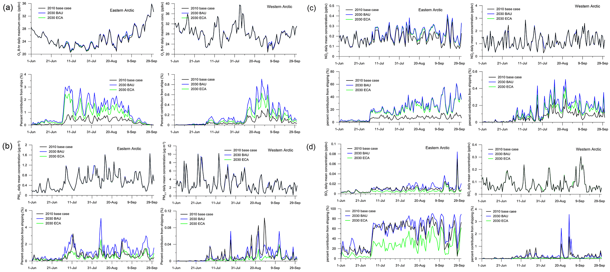
Figure 14(a) Modelled population-weighted O3 concentrations (8 h daily maximum) over the eastern and western Canadian Arctic (top panels) and contributions from Canadian Arctic shipping emissions (bottom panels). (b) Modelled population-weighted PM2.5 concentrations over the eastern and western Canadian Arctic (top panels) and contributions from Canadian Arctic shipping emissions (bottom panels). (c) Modelled population-weighted NO2 concentrations over the eastern and western Canadian Arctic (top panels) and contributions from Canadian Arctic shipping emissions (bottom panels). (d) Modelled population-weighted SO2 concentration over the eastern and western Canadian Arctic (top panels) and contributions from Canadian Arctic shipping emissions (bottom panels).
Table 7Arctic shipping contributions to population-weighted concentrations of criteria pollutants over eastern Canadian Arctic (north of 60∘ N, 60–100∘ W), for the July–August–September period.
It is interesting to compare the above model-based assessment of Arctic shipping emissions on air quality with measurement-based analysis. Aliabadi et al. (2015) conducted an analysis on the air quality measurements collected during the 2013 shipping season from two monitoring stations in the eastern Canadian Arctic: Cape Dorset (on Foxe Peninsula at the southern end of Baffin Island) and Resolute, in Nunavut, both located near Arctic shipping channels. Using back trajectories and high-resolution ship position data, they estimated that ship emissions contributed to cumulated concentrations (equivalent to dosage) of NOx, O3, SO2, and PM2.5 of: 12.9 %–17.5 %, 16.2 %–18.1 %, 16.9 %–18.3 %, and 19.5 %–31.7 %, respectively, at Cape Dorset (southern site); and 1.0 %–7.2 %, 2.9 %–4.8 %, 5.5 %–10.0 %, and 6.5 %–7.2 %, respectively, at Resolute (northern site). This may be loosely compared to the model assessment based on population-weighted concentration above (Table 7), bearing in mind the difference in metrics, as it is also weighted towards small coastal communities. Ship contributions to O3 and PM2.5 concentrations were estimated to be higher based on the measurements than from the model assessment. This may be due in part to the methodology used in Aliabadi et al. (2015), where the concentrations exceeding the deemed “background level” was attributed entirely to ship influence whenever a back trajectory crossed a ship location. In the case of O3 and PM2.5, which are either purely or partly secondary pollutants with relative long lifetimes, this is likely to over attribute ship influence, as the air parcel could well be influenced by other sources as well as ship plumes. In contrast, the ship contributions to NO2 (or NOx in the case of measurement-based analysis) and SO2 were estimated lower from the measurements than from the model assessment. This can also be expected, as the measurement sites were often influenced by local sources (e.g., garbage burning, off-road use of diesel, aeroplane landings and take-offs) which are not represented well in the model simulations. Combined with instrument lower detection limits (LDLs), the background levels in the measurement analysis for NOx and SO2 are much greater than the corresponding modelled background levels, which leads to greater ship contribution (in relative sense) from the model assessment than from the measurements.
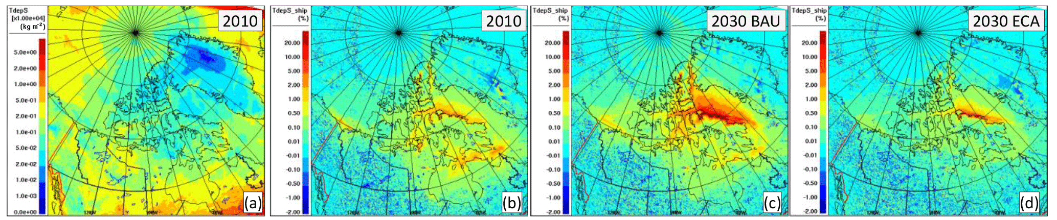
Figure 15(a) Total sulfur deposition over the July–August–September period (accumulated) for the base case (2010); (b) Arctic shipping contribution at current (2010) level; (c) the same as in (b) for the 2030 BAU scenario; (d) the same as in (b) for the 2030 ECA scenario.

Figure 16(a) Total nitrogen deposition over the July–August–September period (accumulated) for the base case (2010); (b) Arctic shipping contribution at current (2010) level; (c) the same as in (b) for the 2030 BAU scenario; (d) the same as in (b) for the 2030 ECA scenario.
5.2 On deposition of S and N
The impacts of Arctic shipping on the deposition of sulfur and nitrogen at current 2010 and projected 2030 levels were also examined in this study. The model computes both dry and wet deposition fluxes of various sulfur- and nitrogen-containing species. They include, for dry deposition, SO2, pSO4, NO, NO2, HNO3, NH3, HONO, RNO3 (organic nitrate), PAN (peroxyacetyl-nitrate), pNO3, pNH4, and for wet deposition, , , , and . The modelled wet deposition includes both “rain-out”, i.e., tracer transfer from cloud water to rain water due to precipitation production (autoconversion, collision, coalescence), and “wash-out”, i.e., below-cloud scavenging of aerosol particles and soluble gases by falling hydrometeors, as described in Gong et al. (2006).
Shown in Figs. 15 and 16 are the modelled total sulfur and nitrogen deposition fluxes accumulated over the JAS period and the contributions from Arctic shipping emissions. The deposition fluxes are shown here for the 2010 base case only, due to the similarity in the geographical distribution patterns between different scenarios, while the shipping contributions are shown for all three scenarios. Overall the deposition fluxes are much lower over the Arctic region compared to lower latitudes. The total sulfur deposition (over the 3-month period) ranges from 0.2 to 0.5 kg S ha−1 over the Canadian sub-Arctic to 0.02–0.05 kg S ha−1 over the Canadian high Arctic; the corresponding ranges for total nitrogen deposition are 0.1–0.5 and 0.01–0.05 kg N ha−1, respectively. For the annual deposition estimate, the base case (2010) simulation was extended to a full year. The annual total depositions of S and N (based on the full-year model simulation) are 0.5–2 kg S ha−1 and 0.2–1 kg N ha−1, respectively, over the Canadian sub-Arctic, and 0.1–0.5 kg S ha−1 and 0.05–0.2 kg N ha−1, respectively, over the Canadian high Arctic (see Fig. S9 in the Supplement). These levels are in general accordance with previous model estimates (e.g., Hole et al., 2009, Vet et al., 2014). The contribution to total sulfur deposition from Arctic shipping is relatively small, below 5 %, at the 2010 base level; however, the contribution from shipping increases to up to 20 % along the coast of Baffin Bay in the 2030 BAU scenario. The 2030 ECA scenario brings down the shipping contribution to generally below the current 2010 level except for along the coast of Baffin Bay, where a major increase in shipping activity from increased economic development is projected. The shipping contribution to total N deposition is comparable to the case of S deposition at the current 2010 level, but it increases substantially under the 2030 BAU scenario, up to 50 %. With assumed ECA-like regulation, the shipping contribution is slightly reduced but is still much greater than at the current 2010 level.
Table 8Percentage contribution from Arctic shipping to surface depositions of sulfur, nitrogen, and elemental carbon (BC) and column loading of EC (BC), by geographical sectors (see Table 1), for the July–August–September period.
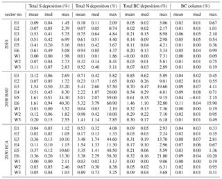
The statistics of shipping contributions to the total depositions of S and N by the nine geographical sectors are shown in Table 8. Similar to the cases of ambient SO2 and NO2, the sectors most affected by Arctic shipping emissions are the four northernmost sectors in the east (E3–E6). However, in contrast to the cases of ambient SO2 and NO2, where Arctic shipping contributions are much more important, the contributions to total depositions of S and N from Arctic shipping are much less substantial. This is in part due to the dominance of wet deposition in the total depositions of S and N (as is discussed later) over the region of interest. The dominance of wet deposition over dry deposition over northern Canada is also found in a recent global assessment study of Vet et al. (2014), and it is consistent with the fact that the area has relatively low emissions and moderate precipitation amounts (particularly during the summer months). While dry deposition is more associated with ambient (or near-surface) concentrations, wet deposition is more associated with concentrations aloft (i.e., at cloud levels and through the vertical column) and hence is more affected by long-range transport and distant sources. Due to its moderate solubility and fast oxidation pathways in the aqueous phase, SO2 can be efficiently scavenged into cloud droplets, oxidized into sulfate, and be transported and deposited (through rain-out) long distances from its sources. Similarly, both NH3 and HNO3 can be readily scavenged by cloud water and both contribute significantly to the wet deposition of N: gaseous NH3 is highly soluble and, once absorbed by cloud water, will mostly be in the form of ammonium ions (); HNO3 is extremely soluble and will quickly dissociate into nitrate ions () once dissolved in cloud water (Seinfeld and Pandis, 1996).
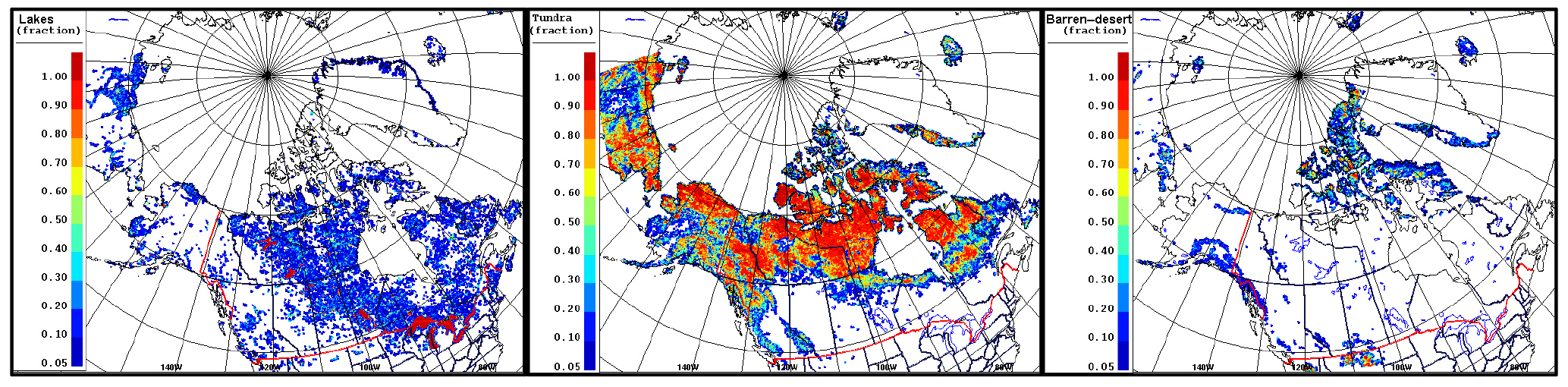
Figure 17Gridded land-cover fractions for lakes, tundra, and barren–desert based on USGS v2.0 at 1 km resolution.
The deposition of S and N is of importance in considering ecosystem impacts, e.g., acidification and eutrophication of terrestrial and aquatic systems (Reuss and Johnson, 1986; Bouwman et al., 2002). To this end, land-cover-weighted deposition fluxes of S and N for three primary land-cover types found in the Canadian Arctic, namely lakes, tundra, and barren–desert, were computed and the contributions to the land-cover-weighted deposition from Arctic shipping are examined. Figure 17 shows the gridded land-cover fractions for the three land-cover types based on the US Geological Survey's (USGS) Global Land Cover Characteristics (GLCC) database at 1 km resolution (see https://lta.cr.usgs.gov/glcc/globdoc2_0, last access: 13 November 2018). Similar to the population-weighted concentration, the land-cover-weighted deposition is calculated as
where fraci, Ai, and depoi are gridded land-cover fraction (for a given land-cover type), grid area, and deposition flux, respectively, at grid cell i.
Table 9Land-cover-weighted deposition of S and N for the eastern Canadian Arctic (60–90∘ N, 60–100∘ W) over the July–August–September period and corresponding contributions from Arctic shipping.
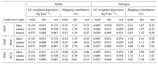
Forsius et al. (2010) estimated critical loads of acidity (S and N) for terrestrial ecosystems north of 60∘ latitude using a simple mass balance (SMB) model and found that in northern North America, the lowest critical loads (or most sensitive regions) occur in eastern Canada. Table 9 shows the land-cover-weighted depositions of S and N (dry and wet, both total and separately) for the eastern Canadian Arctic (60N–90∘ N, 60–100∘ W) over the JAS period and the respective contributions from Arctic shipping. At the current level, land-cover-weighted total S deposition over the eastern Canadian Arctic varies from 73 g ha−1 over barren land to 143 g ha−1 over lakes for the 3-month period. The corresponding numbers for the annual deposition of S over the eastern Canadian Arctic, based on the extended annual simulation (2010 base case), are 288 g ha−1 over barren land, 652 g ha−1 over lakes (see Table S3 in the Supplement), or a range of 18–40 eq ha−1 (assuming that 1 mole of S equals 2 acid equivalents; Bouwman et al., 2002), which is well below the lowest critical load of acidity (based on 5th percentile of the maximum critical load of S) estimated by Forsius et al. (2010) for the area: 200 eq ha−1 a−1 (using an aluminum–base-cation ratio criteria) or 100 eq ha−1 a−1 (using an acid neutralizing capacity criteria, a more stringent measure). Note that caution needs to be taken in interpreting the corresponding deposition values for the 2030 scenarios as there was no projection done for the anthropogenic emissions other than for the marine shipping emissions over Canadian waters for these model runs. The shipping contributions to the total deposition of S to the three land-cover types are small (below 1 %), while the contributions to dry deposition (which is more heavily tied to ambient concentrations) are noticeably greater. As shown in Table 9, the total deposition of S (and N) is dominated by wet deposition in this region. The land-cover-weighted N deposition ranges between 36 g ha−1 (over barren land) and 84 g ha−1 (over lakes) over the JAS period at the present level. Again the annual deposition of N, based on the full-year simulation (see Table S3), ranges between 0.137 kg N ha−1 a−1 (over barren land) and 0.274 kg N ha−1 a−1 (over lakes), or 10–20 eq ha−1 a−1, which is also below the critical load for acidification currently estimated for the region in Forsius et al. (2010) as well as the empirical critical loads for nutrient N of 1–3 kg N ha−1 a−1 for the North America ecoregion of tundra (Pardo et al., 2011; Linder et al., 2013).
The contributions from Arctic shipping to total N deposition for the three land-cover types are simulated as small at the current level, but are predicted to increase significantly under the 2030 scenarios. It should be noted that, although the current depositions of S and N over the Arctic region are low and generally below the existing critical load estimates, with the projected increase in global production of nitrogen needed to meet the growing demand for food and energy, atmospheric emissions and depositions of nitrogen are expected to increase (Galloway et al., 2004; Dentener et al., 2006); this situation combined with the expected increase in shipping activities in Arctic waters could raise the level of deposition to above the critical loads for the region. Furthermore, it is recognized that the current estimates of critical loads for North American Arctic ecosystems are highly uncertain due to a number of factors including limitations in methodology and lack of data (Forsius et al., 2010; Pardo et al., 2011; Linder et al., 2013). Given these considerations, a careful assessment of potential ecosystem impacts from Arctic shipping emissions, particularly in the future context, is warranted.
5.3 On black carbon
Black carbon, formally defined as an ideally light-absorbing substance composed of carbon (Petzold et al., 2013), is a short-lived climate forcer (SLCF): it absorbs solar radiation, influences cloud processes, and alters the melting of snow and ice and, hence, surface albedo (Bond et al., 2013; Flanner et al., 2007). BC is emitted into the atmosphere from a variety of combustion processes, including shipping activities. Although shipping contributes only up to about 2 % of global BC emissions, it may constitute a larger fraction of direct BC emissions in remote regions such as the Arctic, an area with higher sensitivity to carbonaceous emissions due to snow albedo effects (Bond et al., 2013). In our model, BC is represented by the elemental carbon component of the internally mixed aerosols. By its sources and chemical and physical properties represented in the model, the modelled EC is equivalent to BC. In the context of the important radiative effect of BC, the impact of Arctic shipping emissions on both column loading and deposition of BC (or modelled EC) will be assessed here.
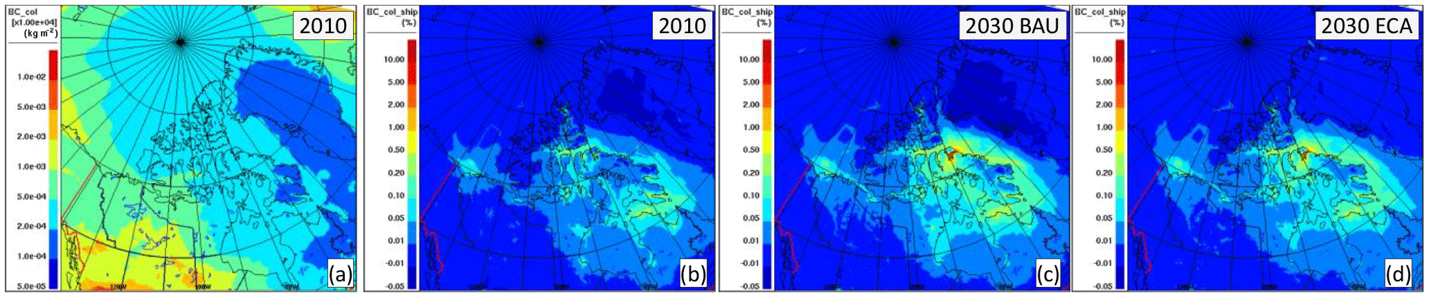
Figure 18Modelled BC column loading (scaled up by 104, in kg m−2) averaged for over the 2010 July–August–September period (a), and relative contributions from Canadian Arctic shipping emissions: (b) 2010 base year, (c) 2030 BAU, and (d) 2030 ECA.
Figure 18 shows the modelled EC (or modelled BC, hereafter) column loadings averaged over the JAS period (2010 base case) and the percentage contributions from Arctic shipping for the 2010 base case, 2030 BAU scenario, and 2030 ECA scenario. The contribution statistics by geographical sectors are included in Table 8 (last column). The modelled, averaged BC column loading over the Canadian Arctic (north of 60∘ N) ranges between 20 and 200 µg m−2 (Fig. 18a), higher over the western Canadian Arctic than the east, where the region is strongly impacted by northern boreal forest fires over western Canada and Alaska during the summer months. A similar range of modelled BC loading over the Arctic is also reported by Eckhardt et al. (2015) in a recent multi-model assessment for simulating BC and sulfate in the Arctic atmosphere. The contribution to BC loading from Canadian Arctic shipping emissions at the 2010 baseline level is limited and localized, generally below 0.1 % on average and up to 2 % over localized areas in the eastern Canadian Arctic (Fig. 18b). In absolute terms, the shipping contribution to BC loading is below 0.1 µg m−2 over most parts of the Canadian Arctic. This is somewhat smaller than the estimate of Ødemark et al. (2012), where the Arctic shipping contribution to the tropospheric BC column is estimated at 0.38 µg m−2 averaged over 60–90∘ N. Noting that the present assessment focuses on the impact of shipping over the Canadian Arctic waters only, as opposed to shipping over the entire Arctic waters (as in the case of Ødemark et al., 2012), the smaller contribution from this assessment is expected, as shipping activities within Canadian Arctic waters constitute only a small portion of overall Arctic shipping activities, e.g., compared to the activities over the Barents Sea, Norwegian Sea, and along southwest coast of Greenland (Arctic Council, 2009; Winther et al., 2014). There is a considerable increase in the contribution to BC loadings from Canadian Arctic shipping emissions in the 2030 BAU scenario of up to 15 % locally, as seen in Fig. 18c and Table 8, particularly over Baffin Bay, in response to projected increases in ship traffic there. Under the 2030 ECA scenario, the modelled shipping contribution to BC loading is slightly reduced from the 2030 BAU level, but it is still significantly greater than that at the current 2010 level (Fig. 18d and Table 8).
The model simulated total (dry + wet) deposition of BC accumulated for the JAS period at the current (2010) level is shown in Fig. 19 along with the percentage contribution from shipping over Canadian Arctic waters under all three scenarios. The contribution statistics by geographical sectors are included in Table 8 (2nd last column). Modelled BC deposition over the Canadian Arctic ranges from up to 50 mg m−2 in the southwest to around 0.5 mg m−2 in the northeast over the 3-month period. The modelled area-averaged BC deposition flux for 60–90∘ N between 50∘ W and 140∘ W is 2.3 mg m−2 over the 3-month period, or 9.2 mg m−2 yr−1, which is within the range of modelled BC deposition fluxes averaged over the Arctic (60∘–90∘ N) from a multi-model assessment of Jiao et al. (2014; see their Fig. 9). The contribution from Canadian Arctic shipping at current levels is mostly between 0.1 % and 0.5 % over the shipping channels and locally up to 5 % (Fig. 19b). Similar to the case of BC column loading discussed above, there is an important increase in the shipping contribution to BC deposition in the 2030 BAU scenario over the east coast of Baffin Island (Fig. 19c). The shipping contribution to BC deposition averaged over the northeast sector E6 increases to 1.5 %, exceeding 30 % locally, under the 2030 BAU scenario (Table 8).
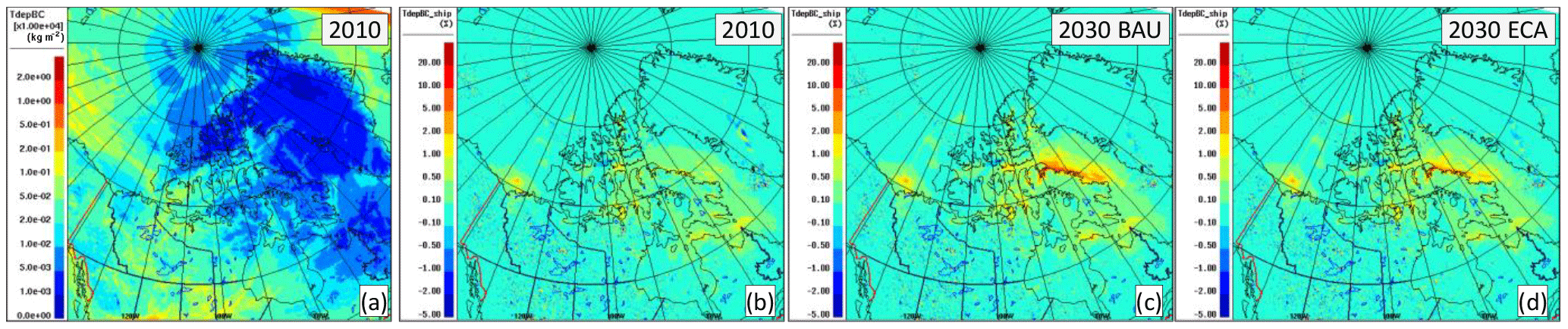
Figure 19Modelled total BC deposition flux (scaled up by 104, in kg m−2) accumulated over the 2010 July–August–September period (a), and relative contributions from Canadian Arctic shipping emissions: (b) 2010 base year, (c) 2030 BAU, and (d) 2030 ECA.
Since BC deposition to ice and snow is of most interest when considering the potential albedo effect, averaged BC deposition fluxes to ice and snow, defined as
(where Fice∕snow is the grid fraction of ice and snow cover), have been computed, and the respective contributions from shipping within Canadian Arctic waters are examined here. Table 10 shows average monthly BC deposition fluxes to ice and snow (total, as well as dry and wet, separately) over the Canadian Arctic region (60–90∘ N, 50–140∘ W) for the three peak shipping months, July–September, and the corresponding shipping contributions. Modelled monthly mean ice and snow cover fields (shown in Fig. 20) are used for this calculation. As shown, the Arctic ice and snow cover recedes progressively through the summer months. The monthly BC deposition to ice and snow is highest in August due to higher precipitation and wet deposition. There is a sharp reduction in September as a result of the combination of a reduction in column BC loading (see Fig. S10 in the Supplement) due to the reduced wildfire events in western Canada in late summer and receding ice and snow cover further to the north (Fig. 20). Again total deposition is largely dominated by the wet component. In general, shipping over Canadian Arctic waters makes only a small contribution to the total BC deposition on Arctic ice and snow; the relative contribution is larger in September due to the reduced impact from wildfire emissions. Proportionally, Arctic shipping makes a greater contribution through dry deposition than through wet deposition over northern regions as the emissions are more likely to be trapped within the stable marine boundary layer and hence have a greater impact on the near-surface atmospheric concentration. Table 10 also includes the shipping contribution to BC deposition to ice and snow in absolute terms. It shows that the shipping contributions are roughly double in the 2030 BAU scenario from present levels. It is interesting to see that dry deposition is playing a bigger role in this increase, particularly for the month of July, reflecting a significant increase in near-surface atmospheric concentration of BC in this scenario.

Table 10Averaged BC deposition on ice and snow over the Canadian Arctic (60–90∘ N, 50–140∘ W), and contributions from shipping over the Canadian Arctic waters.
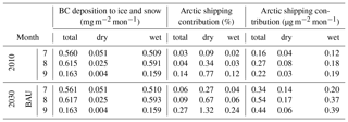
It is seen from this assessment that current shipping emissions over Canadian Arctic waters make relatively small contributions to both BC loading and deposition in the Arctic. However, the contributions are expected to increase in the 2030 scenarios. Assessing the radiative effect from BC loading and deposition on snow attributable to the shipping emissions over the Canadian Arctic waters is beyond the scope of this study. There are existing efforts to assess radiative forcing from specific forcing agents and/or emission sectors mostly using global models with relatively coarse resolutions. For example, a global BC radiative forcing of ∼2 mW m−2 attributable to current international shipping (without the consideration for BC snow albedo effect) was estimated by Eyring et al. (2010); Ødemark et al. (2012) estimated annual mean BC relative forcing attributable to Arctic shipping activities at the present (2004) level to be 0.60 mW m−2 (due to BC in air) and 0.47 mW m−2 (due to BC in snow) averaged over 60–90∘ N. The current understanding is that overall net forcing from the present-day ship emissions of SLCF pollutants is negative due to higher emission of sulfur (Fuglestvedt et al., 2008; Eyring et al., 2010; Ødemark et al., 2012). As seen from this assessment, shipping-induced changes in atmospheric composition and deposition are occurring at regional to local scales (particularly in the Arctic). Climate feedbacks are therefore likely to act at these scales, and hence, climate forcing impact assessments will require modelling undertaken at much finer resolutions than those used in the existing relative forcing and climate impact assessments.
In this study, an on-line air quality forecast model (GEM-MACH) was used for a first regional assessment of the impact of Arctic shipping emissions on air pollution in the Canadian Arctic and northern regions. First, the model's ability to simulate ambient atmospheric compositions in the region of interest was evaluated with available observations. The impacts of Arctic shipping emissions at both present and projected future levels were then assessed based on model sensitivity runs using a detailed marine emission inventory for ships sailing in Canadian waters developed specially for this study.
The adapted GEM-MACH for Arctic is shown to have similar skill in predicting ambient O3 and PM2.5 in the Canadian northern and Arctic regions as the current operational air quality forecast models in North America and Europe. The model is able to simulate the observed ambient O3, and some of the PM components well at the Canadian high Arctic site, Alert. The model has reasonable skill in predicting NO2 and SO2 in the north at a regional scale; at local scales the model prediction depends heavily on emission inputs. The evaluation results indicate large uncertainties in the representation of local emissions in the remote north and the need for improved emission estimates and representation for the oil and gas facilities in northeastern British Columbia and northern Alberta. There is a significant data gap in northern Canada, particularly the eastern Arctic, for air quality monitoring and model evaluation.
Key findings from the model assessment of the impact of Arctic shipping emissions are the following.
-
At the current (2010) level, Arctic shipping emissions contribute to less than 1 % of ambient O3 concentration over the eastern Arctic. This contribution is expected to increase to up to 5 % in the 2030 business-as-usual (BAU) scenario with a broader region of impact.
-
In comparison, the impact of Arctic shipping emission on ambient PM2.5 concentration is more confined to areas close to the shipping channels. Current (2010) levels of Arctic shipping contribute to 1 %–5 % of ambient PM2.5 concentration over the shipping channels and < 0.5 % over land. At the 2030 BAU level, the shipping contribution is expected to increase to 5 %–20 % over the shipping channels.
-
For NO2 and SO2, both primary pollutants, Arctic shipping emissions make significant contributions to ambient concentrations over the eastern Arctic: 10 %–50 % for NO2 and 20 %–100 % for SO2, over shipping channels and coastal regions with close proximity to shipping routes at current (2010) level. The shipping contribution to NO2 concentrations is expected to increase to > 50 % under 2030 BAU, while the increase in the shipping contribution to SO2 concentrations is more moderate due to the anticipated global cap on sulfur in ship fuel that is due to come into effect.
-
Contrasting to the 2030 BAU, the 2030 ECA scenario, i.e., assuming the Canadian Arctic will be designated as an emission control area (as is the case for the east and west coasts of North America), will see a significant reduction in the Arctic shipping contribution to ambient concentrations of SO2 and PM2.5. Particularly, the Arctic shipping contributions to the population-weighted concentration of SO2 and PM2.5 will be brought down to below the current level.
-
Despite the significant contributions to the ambient concentrations of SO2 and NO2, the Arctic shipping contribution to the deposition of total S and N to the Arctic ecosystem is small, < 5 %, at present (2010) level due to the dominance of wet deposition. However, the contribution is expected to increase to up to 20 % for S and 50 % for N under the 2030 BAU scenario.
-
Based on existing estimates of critical loads for northern terrestrial ecosystems, the current S and N deposition to the three dominant land-cover types (tundra, lakes, and barren–desert) in the Canadian Arctic and northern region is well below the lowest critical loads for acidification and eutrophication. However, given the large uncertainty in the current critical load estimates for the Arctic ecosystem, the anticipated increase in atmospheric emissions and deposition of nitrogen globally, and the expected increase in Arctic shipping contribution to the deposition of N to the north, more careful assessment of potential ecosystem impacts from Arctic shipping emissions, particularly in the future context, is needed.
-
The contribution to BC loadings from Canadian Arctic shipping emissions at the 2010 baseline level is limited and localized, generally below 0.1 % on average and up to 2 % over localized areas in the eastern Canadian Arctic. There is a considerable increase in the contribution to the BC loading from the Canadian Arctic shipping emissions in the 2030 BAU scenario, particularly over Baffin Bay with up to 15 % locally, in response to the projected increase in ship traffic there.
-
The contribution to BC deposition from shipping in the Canadian Arctic at current (2010) levels is mostly between 0.1 % and 0.5 % over the shipping channels and locally up to 5 %. Similar to the case of BC column loading, there is an important increase in the shipping contribution to BC deposition in the 2030 BAU scenario over the east coast of Baffin Island. The shipping contribution to BC deposition averaged over the eastern Canadian high Arctic increases to 1.5 %, exceeding 30 % locally.
-
In general, shipping over the Canadian Arctic waters makes a small contribution towards the total BC deposition on Arctic ice and snow (taking into account of the sea-ice cover during the Arctic shipping season). Proportionally, Arctic shipping makes a greater contribution to dry deposition than to wet deposition over the northern regions as the emissions are more likely to be trapped within the stable marine boundary layer and hence have greater impact on the near-surface atmospheric concentration. The analysis shows that shipping contributions to BC deposition fluxes to ice and snow are roughly double in the 2030 BAU scenario from present levels, in response to the projected increase in Arctic shipping activities.
-
It is indicative from this study that shipping-induced changes in atmospheric composition and deposition are at regional to local scales (particularly in the Arctic). Climate feedbacks are consequently likely to act at these scales, thus climate impact assessments will require modelling undertaken at much finer resolutions than those used in the existing radiative forcing and climate impact assessments.
The air quality monitoring data used for model evaluation can be freely downloaded from the respective data repositories: https://open.canada.ca/data/en/dataset/1b36a356-defd-4813-acea-47bc3abd859b (last access: 8 November 2018) for National Air Pollution Surveillance network data (ECCC, 2018); US Environmental Protection Agency Air Quality System Data Mart [internet database] is available at https://aqs.epa.gov/aqsweb/documents/data_mart_welcome.html (last access: 8 November 2018) (US EPA, 2018) for US network data; http://ds.data.jma.go.jp/gmd/wdcgg/cgi-bin/wdcgg/catalogue.cgi?&order=country, (last access: 8 November 2018) (WMO Global Atmosphere Watch, 2018) for the World Data Centre for Greenhouse Gases data. All other data (model simulation output, emission input, including shipping emissions) are available upon request from the corresponding author Wanmin Gong (wanmin.gong@canada.ca). GEM-MACH refers to the atmospheric chemistry library for the GEM numerical atmospheric model, Copyright ©2007–2013 (Air Quality Research Division and National Prediction Operations Division, Environment and Climate Change Canada). This library is free software which can be redistributed and/or modified under the terms of the GNU Lesser General Public License as published by the Free Software Foundation; either version 2.1 of the License, or any later version. The MACH-Arctic (chemistry) code can be downloaded from this Zenodo site: https://doi.org/10.5281/zenodo.1487978 (Beagley et al., 2018), and the GEM (meteorology) code (Canadian Meteorological Centre, 2018) is available for download from https://github.com/mfvalin?tab=repositories (last access: 8 November 2018). The executable for GEM-MACH-Arctic is obtained by providing the chemistry library (MACH-Arctic) to GEM when generating its executable.
The following statistical measures are considered for the model evaluation
in this study, letting M be the vector of model output and O be the vector of
observation (both of N record length), with mean values and ,
respectively.
Mean bias (MB)
Normalized mean bias (NMB)
Root mean square error (RMSE)
Normalized mean square error (NMSE)
Pearson correlation coefficient (r)
The supplement related to this article is available online at: https://doi.org/10.5194/acp-18-16653-2018-supplement.
WG led the model assessment study. WG and SC designed the experiments with inputs from LL, HM, and RH. SRB was responsible for code modifications and model configuration with assistance from WG. MS was responsible for emission processing for the modelling study with help from RMA, SC, and JZ. JC helped with the initial implementation of NA wildfire emissions in the model. PB and JL were responsible for the 2010 Canadian marine shipping emission inventory and the 2030 projection. Model simulations were carried out by SRB and RMA with assistance from SM. SRB performed the majority of the analysis and was assisted by WG. SS and LH were responsible for collecting and processing the air chemistry data from Alert used for the model evaluation. JR helped with post-processing of the model results. WG prepared the manuscript with contributions from all co-authors.
The authors declare that they have no conflict of interest.
We would like to acknowledge ECCC's National Atmospheric Chemistry Database (NAtChem) and Analysis Facility for access to the North America air
monitoring data used for model evaluation in this study. We are thankful to
the agencies in Canada and US for maintaining the networks, in particular
the National Air Pollution Surveillance (NAPS) network in Canada and the US
EPA's Aerometric Information Retrieval System (AIRS) and Air Quality System (AQS) database. The World Data Centre for Greenhouse Gases (WDCGG) and
NOAA's Earth System Research Laboratory (Audra McClure-Begley and Irina Petropavlovskikh) are
gratefully acknowledged for providing the O3 monitoring data at Barrow,
Alaska. We would also like to acknowledge the MACC-II project and Xiaobo
Yang (ECMWF) for processing and providing the 2010 MACC-MOZART reanalysis
data. Monica Hilborn of the Environmental Protection Branch (EPB) at ECCC
diligently reviewed and verified the Canadian marine inventory numbers, and
Hui Peng of EPB at ECCC reviewed the manuscript. We are also grateful to
the GEM-MACH development team at ECCC for technical support.
Edited by: Laurens Ganzeveld
Reviewed by: two anonymous referees
Aliabadi, A. A., Staebler, R. M., and Sharma, S.: Air quality monitoring in communities of the Canadian Arctic during the high shipping season with a focus on local and marine pollution, Atmos. Chem. Phys., 15, 2651–2673, https://doi.org/10.5194/acp-15-2651-2015, 2015.
Aliabadi, A. A., Staebler, R. M., de Grandpré, J., Zadra, A., and Vaillancourt, P. A.: Comparison of Estimated Atmospheric Boundary Layer Mixing Height in the Arctic and Southern Great Plains under Statically Stable Conditions: Experimental and Numerical Aspects, Atmos. Ocean, 54, 60–74, https://doi.org/10.1080/07055900.2015.1119100, 2016a.
Aliabadi, A. A, Staebler, R. M., Liu, M., and Herber, A.: Characterization and parametrization of Reynolds stress and turbulent heat flux in the stably-stratified lower Arctic troposphere using aircraft measurements, Bound.-Lay. Meteorol., 161, 99–126, https://doi.org/10.1007/s10546-016-0164-7, 2016b.
Arctic Council: Arctic Marine Shipping Assessment 2009 Report, Arctic Council, Tromsa, Norway, 194 pp., 2009.
Aulinger, A., Matthias, V., Zeretzke, M., Bieser, J., Quante, M., and Backes, A.: The impact of shipping emissions on air pollution in the greater North Sea region – Part 1: Current emissions and concentrations, Atmos. Chem. Phys., 16, 739–758, https://doi.org/10.5194/acp-16-739-2016, 2016.
Barrie, L. A. and Platt, U.: Arctic tropospheric chemistry, Tellus B, 49, 450–454, 1997.
Beagley, S. R., Gong, W., and GEM-MACH Development Team: GEM-MACH-Arctic rev1484+ (Version v1.0.0), Zenodo, https://doi.org/10.5281/zenodo.1487978, last access: 15 November 2018.
Boé, J., Hall, A., and Qu, X.: September sea-ice cover in the Arctic Ocean projected to vanish by 2100, Nat. Geosci., 2, 341–343, 2009.
Bond, T. C., Doherty, S. J., Fahey, D. W., Forster, P. M., Berntsen, T., DeAngelo, B. J., Flanner, M. G., Ghan, S., Karcher, B., Koch, D., Kinne, S., Kondo, Y., Quinn, P. K., Sarofim, M. C., Schultz, M. G., Schulz, M., Venkataraman, C., Zhang, H., Zhang, S., Bellouin, N., Guttikunda, S. K., Hopke, P. K., Jacobson, M. Z., Kaiser, J. W., Klimon, Z., Lohmann, U., Schwarz, J. P., Shindell, D., Storelvmo, T., Warren, S. G., and Zender, C.: Bounding the role of black carbon in the climate system: A scientific assessment, J. Geophys. Res.-Atmos., 118, 5380–5552, https://doi.org/10.1002/jgrd.50171, 2013.
Bouwman, A. F., van Vuuren, D. P., Derwent, R. G., and Posch, M.: A global analysis of acidification and eutrophication of terrestrial ecosystems, Water Air Soil Poll., 141, 349–382, 2002.
Briggs, G. A.: Plume rise predictions, in: Lectures on Air Pollution and Environmental Impact Analysis, edited by: Haugen, D. A., American Meteorological Society, Boston, MA, USA, 59–111, 1975.
Browse, J., Carslaw, K. S., Schmidt, A., and Corbett, J. J.: Impact of future Arctic shipping on high-latitude black carbon deposition, Geophys. Res. Lett., 40, 4459–4463, https://doi.org/10.1002/grl.50876, 2013.
Buehner, M., Caya, A., Pogson, L., Carrieres, T., and Pestieau, P.: A New Environment Canada Regional Ice Analysis System, Atmos. Ocean, 51, 18–34, https://doi.org/10.1080/07055900.2012.747171, 2013.
Canadian Meteorological Centre: gemdyn and rpnphy repositories, available at: https://github.com/mfvalin?tab=repositories, last access: 8 November 2018.
Charron, M., Polavarapu, S., Buehner, M., Vaillancourt, P. A., Charrette, C., Roch, M., Morneau, J., Garand, L., Aparicio, J. M., MacPherson, S., Pellerin, S., St-James, J., and Heilliette, S.: The stratospheric extension of the Canadian global deterministic medium-range weather forecasting system and its impact on tropospheric forecasts, Mon. Weather Rev., 140, 1924–1944, https://doi.org/10.1175/MWR-D-11-00097.1, 2012.
Corbett, J. J. and Köhler, H. W.: Updated emissions from ocean shipping, J. Geophys. Res., 108, 4650, https://doi.org/10.1029/2003JD003751, 2003.
Côté, J., Gravel, S., Méthot, A., Patoine, A., Roch, M., and Staniforth, A.: The operational CMC–MRB Global Environmental Multiscale (GEM) model, Part I: Design considerations and formulation, Mon. Weather Rev., 126, 1373–1395, 1998a.
Côté, J., Desmarais, J.-G., Gravel, S., Méthot, A., Patoine, A., Roch, M., and Staniforth, A.: The operational CMC–MRB Global Environmental Multiscale (GEM) model, Part II: Results, Mon. Weather Rev., 126, 1397–1418, 1998b.
Dalsøren, S. B., Samset, B. H., Myhre, G., Corbett, J. J., Minjares, R., Lack, D., and Fuglestvedt, J. S.: Environmental impacts of shipping in 2030 with a particular focus on the Arctic region, Atmos. Chem. Phys., 13, 1941–1955, https://doi.org/10.5194/acp-13-1941-2013, 2013.
Dentener, F., Drevet, J., Lamarque, J. F., Bey, I., Eickhout, B., Fiore, A. M., Hauglustaine, D., Horowitz, W. W., Krol, M., Kulshrestha, U. C., Lawrence, M., Galy-Lacaux, C., Rast, S., Shindell, D., Stevenson, D., Van Noije, T., Atherton, C., Bell, N., Bergman, D., Butler, T., Cofala, J., Collins, B., Doherty, R., Ellingsen, K., Galloway, J., Gausee, M., Montanaro, V., Müller, J. F., Pitari, G., Rodriguez, J., Sanderson, M., Solmon, F., Strahan, S., Schultz, M., Sudo, K., Szopa, S., and Wild, O.: Nitrogen and sulfur deposition on regional and global scales: a multimodel evaluation, Global Biogeochem. Cy., 20, GB4003, https://doi.org/10.1029/2005GB002672, 2006.
ECCC: National Air Pollution Surveillance network data, available at: https://open.canada.ca/data/en/dataset/1b36a356-defd-4813-acea-47bc3abd859b, last access: 8 November 2018.
Eckhardt, S., Quennehen, B., Olivié, D. J. L., Berntsen, T. K., Cherian, R., Christensen, J. H., Collins, W., Crepinsek, S., Daskalakis, N., Flanner, M., Herber, A., Heyes, C., Hodnebrog, Ø., Huang, L., Kanakidou, M., Klimont, Z., Langner, J., Law, K. S., Lund, M. T., Mahmood, R., Massling, A., Myriokefalitakis, S., Nielsen, I. E., Nøjgaard, J. K., Quaas, J., Quinn, P. K., Raut, J.-C., Rumbold, S. T., Schulz, M., Sharma, S., Skeie, R. B., Skov, H., Uttal, T., von Salzen, K., and Stohl, A.: Current model capabilities for simulating black carbon and sulfate concentrations in the Arctic atmosphere: a multi-model evaluation using a comprehensive measurement data set, Atmos. Chem. Phys., 15, 9413–9433, https://doi.org/10.5194/acp-15-9413-2015, 2015.
Emmons, L. K., Arnold, S. R., Monks, S. A., Huijnen, V., Tilmes, S., Law, K. S., Thomas, J. L., Raut, J.-C., Bouarar, I., Turquety, S., Long, Y., Duncan, B., Steenrod, S., Strode, S., Flemming, J., Mao, J., Langner, J., Thompson, A. M., Tarasick, D., Apel, E. C., Blake, D. R., Cohen, R. C., Dibb, J., Diskin, G. S., Fried, A., Hall, S. R., Huey, L. G., Weinheimer, A. J., Wisthaler, A., Mikoviny, T., Nowak, J., Peischl, J., Roberts, J. M., Ryerson, T., Warneke, C., and Helmig, D.: The POLARCAT Model Intercomparison Project (POLMIP): overview and evaluation with observations, Atmos. Chem. Phys., 15, 6721–6744, https://doi.org/10.5194/acp-15-6721-2015, 2015.
Environment and Climate Change Canada (ECCC): Marine Emission Inventory Tool (MEIT) version 4.3.1, 2015.
Environment and Climate Change Canada and Alberta Environment and Parks (ECCC & AEP): Joint Oil Sands Monitoring Program Emissions Inventory Compilation Report, 146 pp., https://open.alberta.ca/publications/9781460125658 (last access: 14 November 2018), 2016.
Eyring, V., Köhler, H. W., van Aardenne, J., and Lauer, A.: Emissions from international shipping: 1. The last 50 years, J. Geophys. Res., 110, D17305, https://doi.org/10.1029/2004JD005619, 2005a.
Eyring, V., Köhler, H. W., Lauer, A., and Lemper, B.: Emissions from international shipping: 2. Impact of future technologies on scenarios until 2050, J. Geophys. Res., 110, D17301, https://doi.org/10.1029/2004JD005620, 2005b.
Eyring, V., Isaksen, I. S. A., Berntsen, T., Collins, W. J., Corbett, J. J., Endresen, O., Grainger, R. G., Moldanova, J., Schlager, H., and Stevenson, D. S.: Transport impacts on atmosphere and climate: Shipping, Atmos. Environ., 44, 4735–4771, 2010.
Flanner, M. G., Zender, C. S., Randerson, J. T., and Rasch, P. J.: Present-day climate forcing and response from black carbon in snow, J. Geophys. Res., 112, D11202, https://doi.org/10.1029/2006JD008003, 2007.
Forsius, M., Posch, M., Aherne, J., Reinds, G. J., Christensen, J., and Hole, L.: Assessing the Impacts of Long-Range Sulfur and Nitrogen Deposition on Arctic and Sub-Arctic Ecosystems, Ambio, 39, 136–147, https://doi.org/10.1007/s13280-010-0022-7, 2010.
Galloway, J. N., Dentener, F. J., Capone, D. G., Boyer, E. W., Howarth, R. W., Seitzinger, S. P., Asner, G. P., Cleveland, C. C., Green, P. A., Holland, E. A., Karl, D. M., Michales, A. F., Porter, J .H., Townsend, A. R., and Vorosmarty, C. J.: Global and regional nitrogen cycles: past, present and future, Biogeochemistry, 70, 153–226, 2004.
Gong, S. L., Barrie, L. A., and Lazare, M.: Canadian Aerosol Module (CAM): a size-segregated simulation of atmospheric aerosol processes for climate and air quality models 2, Global sea-salt aerosol and its budgets, J. Geophys. Res., 107, 4779, https://doi.org/10.1029/2001JD002004, 2003.
Gong, W., Dastoor, A. P., Bouchet, V. S., Gong, S.-L., Makar, P. A., Moran, M. D., Pabla, B., Ménard, S., Crevier, L.-P., Cousineau, S., and Venkatesh, S.: Cloud processing of gases and aerosols in a regional air quality model (AURAMS), Atmos. Res., 82, 248–275, 2006.
Gong, W., Beagley, S. R., Zhang, J., Cousineau, S., Chen, J., Sassi, M., Munoz-Alpizar, R., Morrison, H., Lyons, L., and Bellavance, P.: Modelling regional air quality in the Canadian Arctic: Impact of North American wildfire and Arctic shipping emissions, in: Air Pollution Modelling and Its Application XXIV, edietd by: Steyn, D. G. and Chaumerliac, N., Springer, Switzerland, 301–306, 2016.
Gordon, M., Makar, P. A., Staebler, R. M., Zhang, J., Akingunola, A., Gong, W., and Li, S.-M.: A comparison of plume rise algorithms to stack plume measurements in the Athabasca oil sands, Atmos. Chem. Phys., 18, 14695–14714, https://doi.org/10.5194/acp-18-14695-2018, 2018.
Granier, C., Niemeier, U., Jungclaus, J. H., Emmons, L., Hess, P., Lamarque, J.-F., Walters, S., and Brasseur, G. P.: Ozone pollution from future ship traffic in the Arctic northern passages, Geophys. Res. Lett., 33, L13807, https://doi.org/10.1029/2006GL026180, 2006.
Haas, C. and Howell, S. E. L.: Ice thickness in the Northwest Passage, Geophys. Res. Lett., 42, 7673–7680, https://doi.org/10.1002/2015GL065704, 2015.
Helmig, D., Ganzeveld, L., Butler, T., and Oltmans, S. J.: The role of ozone atmosphere-snow gas exchange on polar, boundary-layer tropospheric ozone – a review and sensitivity analysis, Atmos. Chem. Phys., 7, 15–30, https://doi.org/10.5194/acp-7-15-2007, 2007a.
Helmig, D., Oltmansb, S. J., Carlsona, D., Lamarquec, J.-F., Jonesd, A., Labuschagnee, C., Anlauff, K., and Hayden, K.: A review of surface ozone in the polar regions, Atmos. Environ., 41, 5138–5161, 2007b.
Hogrefe, C., Civerolo, K. L., Hao, W., Ku, J.-Y., Zalewsky, E. E., and Sistla, G.: Rethinking the assessment of photochemical modeling systems in air quality planning applications, JAPCA J. Air Waste MA, 58, 1086–1099, 2008.
Hole, L. R., Christensen, J. H., Ruoho-Airola, T., Tørseth, K., Ginzburg, V., and Glowacki, P.: Past and future trends in concentrations of sulphur and nitrogen compounds in the Arctic, Atmos. Environ. 43, 928–939, 2009.
Im, U., Bianconi, R., Solazzo, E., Kioutsioukis, I., Badia, A., Balzarini, A., Baro, R., Bellasio, R., Brunner, D., Chemel, C., Curci, G., Flemming, J., Forkel, R., Giordano, L., Jimenez-Guerrero, P., Hirtl, M., Hodzic, A., Honzak, L., Jorba, O., Knote, C., Kuenen, J. J. P., Makar, P. A., Manders-Groot, A., Neal, L., Perez, J. L., Pirovano, G., Pouliot, G., San Jose, R., Savage, N., Schroder, W., Sokhi, R.S., Syrakov, D., Torian, A., Tuccella, P., Werhahn, K., Wolke, R., Yahya, K., Zabkar, R., Zhang, Y., Zhang, J., Hogrefe, C., and Galmarini, S.: Evaluation of operational online-coupled regional air quality models over Europe and North America in the context of AQMEII phase 2, Part I: ozone, Atmos. Environ., 115, 404–420, 2015a.
Im, U., Bianconi, R., Solazzo, E., Kioutsioukis, I., Badia, A., Balzarini, A., Baro, R., Bellasio, R., Brunner, D., Chemel, C., Curci, G., Denier van der Gon, H. A. C., Flemming, J., Forkel, R., Giordano, L., Jimenez-Guerrero, P., Hirtl, M., Hodzic, A., Honzak, L., Jorba, O., Knote, C., Makar, P. A., Manders-Groot, A., Neal, L., Perez, J. L., Pirovano, G., Pouliot, G., San Jose, R., Savage, N., Schroder, W., Sokhi, R. S., Syrakov, D., Torian, A., Tuccella, P., Werhahn, K., Wolke, R., Yahya, K., Zabkar, R., Zhang, Y., Zhang, J., Hogrefe, C., and Galmarini, S.: Evaluation of operational online-coupled regional air quality models over Europe and North America in the context of AQMEII phase 2, Part II: particulate matter, Atmos. Environ., 115, 421–441, 2015b.
Inness, A., Baier, F., Benedetti, A., Bouarar, I., Chabrillat, S., Clark, H., Clerbaux, C., Coheur, P., Engelen, R. J., Errera, Q., Flemming, J., George, M., Granier, C., Hadji-Lazaro, J., Huijnen, V., Hurtmans, D., Jones, L., Kaiser, J. W., Kapsomenakis, J., Lefever, K., Leitão, J., Razinger, M., Richter, A., Schultz, M. G., Simmons, A. J., Suttie, M., Stein, O., Thépaut, J.-N., Thouret, V., Vrekoussis, M., Zerefos, C., and the MACC team: The MACC reanalysis: an 8 yr data set of atmospheric composition, Atmos. Chem. Phys., 13, 4073–4109, https://doi.org/10.5194/acp-13-4073-2013, 2013.
Innovation Maritime and SNC-Lavalin Environment: Arctic Marine Emission Inventory – Final Report, Prepared for Transport Canada, Transportation Development Centre, Transport Canada, Ottawa, Canada, 2013.
Ivy, D., Mulholland, J. A., and Russell, A. G.: Development of Ambient Air Quality Population-Weighted Metrics for Use in Time-Series Health Studies, JAPCA J. Air Waste MA, 58, 711–720, https://doi.org/10.3155/1047-3289.58.5.711, 2008.
Janssens-Maenhout, G., Dentener, F., van Aardenne, J., Monni, S., Pagliari, V., Orlandini, L., Klimont, Z., Kurokawa, J., Akimoto, H., Ohara, T., Wankmüller, R., Battye, B., Grano, D., Zuber, A., and Keating, T.: EDGAR-HTAP: a harmonized gridded air pollution emission dataset based on national inventories, EUR 25229 EN Report, ISBN 978-92-79-23122-3, ISSN 1018–5593, https://doi.org/10.2788/14069, 2012.
Jiao, C., Flanner, M. G., Balkanski, Y., Bauer, S. E., Bellouin, N., Berntsen, T. K., Bian, H., Carslaw, K. S., Chin, M., De Luca, N., Diehl, T., Ghan, S. J., Iversen, T., Kirkevåg, A., Koch, D., Liu, X., Mann, G. W., Penner, J. E., Pitari, G., Schulz, M., Seland, Ø., Skeie, R. B., Steenrod, S. D., Stier, P., Takemura, T., Tsigaridis, K., van Noije, T., Yun, Y., and Zhang, K.: An AeroCom assessment of black carbon in Arctic snow and sea ice, Atmos. Chem. Phys., 14, 2399–2417, https://doi.org/10.5194/acp-14-2399-2014, 2014.
Jones, J. M., Hogrefe, C., Henry, R. F., Ku, J.-Y., and Sistla, G.: An Assessment of the Sensitivity and Reliability of the Relative Reduction Factor (RRF) Approach in the Development of 8-hr Ozone Attainment Plans. JAPCA J. Air Waste MA, 55, 13–19, 2005.
Larkin, N. K., O'Neill, S. M., Solomon, R., Raffuse, S., Strand, T., Sullivan, D., Krull, C., Rorig, M., Peterson, J., and Ferguson, S. A.: The BlueSky smoke modeling framework, Int. J. Wildland Fire 18, 906–920, https://doi.org/10.1071/WF07086, 2009.
Lee, B. S., Alexander, M. E., Hawkes, B. C., Lynham, T. J., Stocks, B. J., and Englefield, P.: Information systems in support of wildland fire management decision-making in Canada, Comput. Electron. Agr. 37, 185–198, https://doi.org/10.1016/S0168-1699(02)00120-5, 2002.
Linder, G., Brumbaugh, W., Neitlich, P., and Little, E.: Atmospheric Deposition and Critical Loads for Nitrogen and Metals in Arctic Alaska: Review and Current Status, Open Journal of Air Pollution, 2, 76–99, 2013.
Mahmud, A., Hixson, M., and Kleeman, M. J.: Quantifying population exposure to airborne particulate matter during extreme events in California due to climate change, Atmos. Chem. Phys., 12, 7453–7463, https://doi.org/10.5194/acp-12-7453-2012, 2012.
Mahrt, L.: Modelling the depth of the stable boundary-layer, Bound.-Lay. Meteorol., 21, 3–19, 1981.
Marelle, L., Thomas, J. L., Raut, J.-C., Law, K. S., Jalkanen, J.-P., Johansson, L., Roiger, A., Schlager, H., Kim, J., Reiter, A., and Weinzierl, B.: Air quality and radiative impacts of Arctic shipping emissions in the summertime in northern Norway: from the local to the regional scale, Atmos. Chem. Phys., 16, 2359–2379, https://doi.org/10.5194/acp-16-2359-2016, 2016.
Moran, M. D., Menard, S., Talbot, D., Huang, P., Makar, P. A., Gong, W., Landry, H., Gravel, S., Gong, S., Crevier, L.-P., Kallaur, A., and Sassi, M.: Particulate-matter forecasting with GEM-MACH15, a new Canadian air-quality forecast model, in: Air Pollution Modelling and Its Application XX, edited by: Steyn, D. G. and Rao, S. T., Springer, Dordrecht, the Netherlands, 289–292, 2010.
Moran, M. D., Chen, J., Ménard, S., Pavlovic, R., Landry, H., Beaulieu, P.-A., Gilbert, S., Makar, P. A., Gong, W., Stroud, C., Kallaur, A., Robichaud, A., Gong, S., and Anselmo, D.: Two years of operational AQ forecasting with GEM-MACH15: A look back and a look ahead, 10th CMAS Conference, 24–26 October, Chapel Hill, NC, USA, 7 pp., http://www.cmascenter.org/conference/2011/abstracts/moran_two_years_2011.pdf, 2011.
Moran, M. D., Zheng, Q., Zhang, J., and Pavlovic, R.: Regional Air Quality Deterministic Prediction System (RAQDPS), Technical Note, http://collaboration.cmc.ec.gc.ca/cmc/cmoi/product_guide/docs/lib/op_systems/doc_opchanges/Technical_Note_GEM-MACH10_v1.5.3+SET2.1.1_Emissions_9Nov2015.pdf, 2015.
Ødemark, K., Dalsøren, S. B., Samset, B. H., Berntsen, T. K., Fuglestvedt, J. S., and Myhre, G.: Short-lived climate forcers from current shipping and petroleum activities in the Arctic, Atmos. Chem. Phys., 12, 1979–1993, https://doi.org/10.5194/acp-12-1979-2012, 2012.
Pardo, L. H., Fenn, M. E., Goodale, C. L., Geiser, L. H., Driscoll, C. T., Allen, E. B., Baron, J. S., Bobbink, R., Bowman, W. D., Clark, C. M., Emmett, B., Gilliam, F. S., Greaver, T. L., Hall, S. J., Lilleskov, E. A., Liu, L. L., Lynch, J. A., Nadelhoffer, K. J., Perakis, S. S., Robin-Abbott, M. J., Stoddard, J. L., Weathers, K. C., and Dennis, R. L.: Effects of Nitrogen Deposition and Empirical Nitrogen Critical Loads for Ecoregions of the United States, Ecol. Appl., 21, 3049–3082, 2011.
Pavlovic, R., Chen, J., Anderson, K., Moran, M. D., Beaulieu, P.-A., Davignon, D., Cousineau, S.: The FireWork Air Quality Forecast System with Near-Real-Time Biomass Burning Emissions: Recent Developments and Evaluation of Performance for the 2015 North American Wildfire Season, JAPCA J. Air Waste MA, 66, 819–841, https://doi.org/10.1080/10962247.2016.1158214, 2016.
Peters, G. P., Nilssen, T. B., Lindholt, L., Eide, M. S., Glomsrød, S., Eide, L. I., and Fuglestvedt, J. S.: Future emissions from shipping and petroleum activities in the Arctic, Atmos. Chem. Phys., 11, 5305–5320, https://doi.org/10.5194/acp-11-5305-2011, 2011.
Petzold, A., Ogren, J. A., Fiebig, M., Laj, P., Li, S.-M., Baltensperger, U., Holzer-Popp, T., Kinne, S., Pappalardo, G., Sugimoto, N., Wehrli, C., Wiedensohler, A., and Zhang, X.-Y.: Recommendations for reporting “black carbon” measurements, Atmos. Chem. Phys., 13, 8365–8379, https://doi.org/10.5194/acp-13-8365-2013, 2013.
Reuss, J. O. and Johnson, D. W.: Acid deposition and the acidification of soils and waters, Springer, New York, USA, https://doi.org/10.1007/978-1-4419-8536-1; Series ISSN 0070-8356, 1986.
Seinfeld, J. H. and Pandis, S. N.: Atmospheric chemistry and physics: From air pollution to climate change, John Wiley & Sons, Inc., New York, Germany, ISBN 0-471-17815-2, 1996.
Serreze, M. C., Holland, M. M., and Stroeve, J.: Perspectives on the Arctic's shrinking sea-ice cover, Science, 315, 1533–1536, 2007.
Sharma, S., Lavoue, D., Cachier, H., Barrie, L. A., and Gong, S. L.: Long-term trends of the black carbon concentrations in the Canadian Arctic, J. Geophys. Res., 109, D15203, https://doi.org/10.1029/2003JD004331, 2004.
Sharma, S., Leaitch, W. R., Huang, L., Veber, D., Kolonjari, F., Zhang, W., Hanna, S. J., Bertram, A. K., and Ogren, J. A.: An evaluation of three methods for measuring black carbon in Alert, Canada, Atmos. Chem. Phys., 17, 15225–15243, https://doi.org/10.5194/acp-17-15225-2017, 2017.
Shindell, D. T., Chin, M., Dentener, F., Doherty, R. M., Faluvegi, G., Fiore, A. M., Hess, P., Koch, D. M., MacKenzie, I. A., Sanderson, M. G., Schultz, M. G., Schulz, M., Stevenson, D. S., Teich, H., Textor, C., Wild, O., Bergmann, D. J., Bey, I., Bian, H., Cuvelier, C., Duncan, B. N., Folberth, G., Horowitz, L. W., Jonson, J., Kaminski, J. W., Marmer, E., Park, R., Pringle, K. J., Schroeder, S., Szopa, S., Takemura, T., Zeng, G., Keating, T. J., and Zuber, A.: A multi-model assessment of pollution transport to the Arctic, Atmos. Chem. Phys., 8, 5353–5372, https://doi.org/10.5194/acp-8-5353-2008, 2008.
Sirois, A. and Barrie, L. A.: Arctic lower tropospheric aerosol trends and composition at Alert, Canada: 1980–1995, J. Geophys. Res., 104, 11599– 11618, 1999.
SNC-Lavalin Environment: 2010 national marine emission inventory for Canada. Final report prepared for Environment Canada, 351 St. Joseph Boulevard, Place Vincent Massey, Gatineau, Quebec, https://projects.eao.gov.bc.ca/api/document/58bf02ee7b72fa001cf1f270/fetch, 2012.
Stockwell, W. R. and Lurmann, F. W.: Intercomparison of the ADOM and RADM gas-phase chemical mechanisms. Electrical Power Research Institute Topical Report. EPRI, 3412 Hillview Avenue, Paolo Alto, CA, USA, 254 pp., 1989.
US Environmental Protection Agency (US EPA): Air Quality System Data Mart [internet database], available at: https://aqs.epa.gov/aqsweb/documents/data_mart_welcome.html, last access: 13 November 2018.
Val Martin, M., Logan, J. A., Kahn, R. A., Leung, F.-Y., Nelson, D. L., and Diner, D. J.: Smoke injection heights from fires in North America: analysis of 5 years of satellite observations, Atmos. Chem. Phys., 10, 1491–1510, https://doi.org/10.5194/acp-10-1491-2010, 2010.
Vet, R., Artz, R. S., Carou, S., Shawa, M., Ro, C.-U., Aas, W., Baker, A., Bowersox, V. C., Dentener, F., Galy-Lacaux, C., Hou, A., Pienaar, J. J., Gillett, R., Forti, M. C., Gromov, S., Hara, H., Khodzher, T., Mahowald, N. M., Nickovic, S., Rao, P. S. P., and Reid, N. W.: A global assessment of precipitation chemistry and deposition of sulfur, nitrogen, sea salt, base cations, organic acids, acidity and pH, and phosphorus, Atmos. Environ., 93, 3–100, 2014.
Viana, M., Hammingh, P., Colette, A., Querol, X., Degraeuwe, B., de Vlieger, I., and van Aardenne, J.: Impact of maritime transport emissions on coastal air quality in Europe, Atmos. Environ., 90, 96–105, 2014.
Vinken, G. C. M., Boersma, K. F., Jacob, D. J., and Meijer, E. W.: Accounting for non-linear chemistry of ship plumes in the GEOS-Chem global chemistry transport model, Atmos. Chem. Phys., 11, 11707–11722, https://doi.org/10.5194/acp-11-11707-2011, 2011.
Wang, M. and Overland, J. E.: A sea ice free summer Arctic within 30 years?, Geophys. Res. Lett., 36, L07502, https://doi.org/10.1029/2009GL037820, 2009.
Willis, M. D., Burkart, J., Thomas, J. L., Köllner, F., Schneider, J., Bozem, H., Hoor, P. M., Aliabadi, A. A., Schulz, H., Herber, A. B., Leaitch, W. R., and Abbatt, J. P. D.: Growth of nucleation mode particles in the summertime Arctic: a case study, Atmos. Chem. Phys., 16, 7663–7679, https://doi.org/10.5194/acp-16-7663-2016, 2016.
Winther, M., Christensen, J. H., Plejdrup, M. S., Ravn, E. S., Eriksson, Ó. F., and Kristensen, H. O.: Emission inventories for ships in the arctic based on satellite sampled AIS data, Atmos. Environ., 91, 1–14, 2014.
WMO Global Atmosphere Watch: World Data Centre for Greenhouse Gases data, available at: http://ds.data.jma.go.jp/gmd/wdcgg/cgi-bin/wdcgg/catalogue.cgi?&order=country, last access: 13 November 2018.
Zhang, J., Moran, M. D., Zheng, Q., Makar, P. A., Baratzadeh, P., Marson, G., Liu, P., and Li, S.-M.: Emissions preparation and analysis for multiscale air quality modeling over the Athabasca Oil Sands Region of Alberta, Canada, Atmos. Chem. Phys., 18, 10459–10481, https://doi.org/10.5194/acp-18-10459-2018, 2018.
- Abstract
- Introduction
- The 2010 Canadian national marine shipping inventory – Arctic shipping activities (current and projections)
- Modelling system and simulation setup
- Model evaluation – 2010 base case
- Impact of shipping emissions on Arctic air pollution
- Summary and conclusions
- Code and data availability
- Appendix A
- Author contributions
- Competing interests
- Acknowledgements
- References
- Supplement