Surface fluxes of bromoform and dibromomethane over the tropical western Pacific inferred from airborne in situ measurements

We infer surface fluxes of bromoform (CHBr₃) and dibromoform (CH₂Br₂) from aircraft observations over the western Pacific using a tagged version of the GEOS-Chem global 3-D atmospheric chemistry model and a maximum a posteriori inverse model. Using GEOS-Chem (GC) as an intermediary, we find that the distribution of a priori ocean emissions of these gases are reasonably consistent with observed atmospheric mole fractions of CHBr₃ (r=0.62) and CH₂Br₂ (r=0.38). These a priori emissions result in a positive model bias in CHBr₃ peaking in the marine boundary layer, but reproduce observed values of CH₂Br₂ with no significant bias by virtue of its longer atmospheric lifetime. Using GEOS-Chem, we find that observed variations in atmospheric CHBr₃ are determined equally by sources over the western Pacific and those outside the study region, but observed variations in CH₂Br₂ are determined mainly by sources outside the western Pacific. Numerical closed-loop experiments show that the spatial and temporal distribution of boundary layer aircraft data have the potential to substantially improve current knowledge of these fluxes, with improvements related to data density. Using the aircraft data, we estimate aggregated regional fluxes of $\mathrm{3.6}\pm \mathrm{0.3}\times {\mathrm{10}}^{\mathrm{8}}$ and $\mathrm{0.7}\pm \mathrm{0.1}\times {\mathrm{10}}^{\mathrm{8}}$ g month⁻¹ for CHBr₃ and CH₂Br₂ over 130–155^∘E and 0–12^∘ N, respectively, which represent reductions of 20 %–40 % of the prior inventories by Ordóñez et al. (2012) and substantial spatial deviations from different a priori inventories. We find no evidence to support a robust linear relationship between CHBr₃ and CH₂Br₂ oceanic emissions, as used by previous studies. We find that over regions with dense observation coverage, our choice of a priori inventory does not significantly impact our reported a posteriori flux estimates.

1 Introduction

The role of halogens in the catalytic destruction of stratospheric ozone is well established (WMO, 2014). The anthropogenic contribution to the inorganic halogen budget continues to decline in the stratosphere as a result of the Montreal protocol. A consequence of this decline is that very short-lived substances (VSLSs), halogenated compounds with e-folding lifetimes typically much less than 6 months, now represent a proportionally greater source of stratospheric halogens. The wide range of VSLS atmospheric lifetimes allows at least some of the emitted material to reach the upper troposphere, particularly over geographical regions where there is rapid, deep convection (Penkett et al., 1998; Yang et al., 2005; Warwick et al., 2006; Levine et al., 2007; Pisso et al., 2010; Hosking et al., 2010; Carpenter et al., 2014; Hossaini et al., 2016a; Butler et al., 2018). Here, we use aircraft observations of bromoform (CHBr₃) and dibromomethane (CH₂Br₂) collected over the western Pacific Ocean to infer, using an inverse model, the magnitude and distribution of ocean emissions of these gases.

There is a wide range of VSLSs that are beginning to limit the recovery of stratospheric ozone (e.g. Read et al., 2008; Hossaini et al., 2015; Oman et al., 2016). Chlorine VSLSs are typically dominated by anthropogenic sources, but the fraction depends on the species (Hossaini et al., 2016b). Their natural sources include biomass burning, phytoplankton production and soils. Iodine and bromine VSLSs have predominately natural sources. Iodine VSLSs are mainly from ocean production processes, but with lifetimes of only a few days, they are too reactive to be transported out of the marine boundary layer in large quantities. Bromine VSLSs are also mainly from natural ocean sources (Gschwend et al., 1985; Manley et al., 1992; Sturges et al., 1992; Tokarczyk et al., 1994; Warwick et al., 2006; Carpenter and Liss, 2000, 2009; Palmer et al., 2009; Quack and Suess, 1999; Quack and Wallace, 2003; Quack et al., 2007; Butler et al., 2007; Leedham et al., 2013). The most abundant bromine VSLS species are CHBr₃ and CH₂Br₂. Together they account for about 80 % of bromine VSLSs in the marine boundary layer (Law and Sturges, 2007; O'Brien et al., 2009; Hossaini et al., 2013). The local atmospheric lifetime for CHBr₃, determined by OH oxidation (76 days) and photolysis (36 days), is 24 days. CH₂Br₂ has a longer atmospheric lifetime of about 123 days, determined primarily by OH oxidation (123 days) and to a much lesser extent by photolysis (5000 days). Their lifetimes are sufficiently long such that these natural halogenated compounds can be transported to the upper troposphere.

Previous measurement campaigns have reported that bromine VSLS and their degradation products represent 2–8 pptv of stratospheric inorganic bromine (e.g. Dorf et al., 2008; Salawich et al., 2010). Complementary model simulations of atmospheric chemistry and transport, driven by a priori ocean emission inventories, report similar values (2–7 pptv) that are determined mainly by localized regions of active ocean biology that coincide with strong convection. Example regions the include western Pacific Ocean, the tropical Indian Ocean and off the Pacific coast of Mexico. These model calculations also suggest that 15 %–75 % of the stratospheric bromine budget from bromine VSLSs is delivered by the direct transport of the emitted halogenated compounds (Liang et al., 2010; Hossaini et al., 2016a; Aschmann et al., 2009). The large range of values reflects uncertainty in ocean emissions, model transport, and the wet deposition of degradation products in the upper troposphere and lower stratosphere.

Current knowledge of ocean emissions of CHBr₃ and CH₂Br₂ is poorly constrained by the sparse measurements. Bottom-up and top-down methods have been used to estimate global CHBr₃ and CH₂Br₂ emissions. The bottom-up approach assumes local flux estimates are representative of larger spatial scales. Ship-borne air–sea flux observations with limited spatial and temporal coverage are extrapolated over ocean basins (e.g. Quack and Wallace, 2003; Carpenter and Liss, 2000; Butler et al., 2007; Ziska et al., 2013). Poor observation coverage results in fluxes that rely heavily on assumptions used for extrapolation (Stemmler et al., 2015).

The top-down method, in this application, uses an atmospheric chemistry transport model to describe the relationship between emissions and the atmospheric measurements. The model emissions are fitted to the observations by adjusting their magnitude until the discrepancy between the model and observed atmospheric measurements is minimized. This fitting can be achieved using heuristic techniques or more established Bayesian optimization methods (e.g. Liang et al., 2010; Ordóñez et al., 2012; Ashfold et al., 2014; Russo et al., 2015). The short atmospheric lifetime of CHBr₃ poses particular difficulties for the top-down approach because atmospheric mole fractions are highly variable (Ashfold et al., 2014). Some studies have introduced (explicitly or implicitly) a simple linear correlation between CHBr₃ and CH₂Br₂ emissions to provide an additional constraint on the CHBr₃ flux estimate (e.g. Liang et al., 2010; Ordóñez et al., 2012). This approach, however, is then subject to errors associated with the assumption about the correlation. As with the bottom-up method, the top-down method is subject to errors due to poor spatial and temporal coverage of the observations. By virtue of various assumptions made (and justified) by individual studies, the resulting bottom-up and top-down CHBr₃ and CH₂Br₂ fluxes are significantly different (e.g. Hossaini et al., 2016a). For example, the estimated global CHBr₃ annual emissions range from 216 Tg (Ziska et al., 2013) to 530 Tg (Ordóñez et al., 2012).

We use data from two coordinated aircraft campaigns over the western Pacific during 2014 to infer regional emission estimates of CHBr₃ and CH₂Br₂ for the campaign period using a Bayesian inverse model. The Coordinated Airborne Studies in the Tropics (CAST; Harris et al., 2017), and Convective Transport of Active Species in the Tropics (CONTRAST; Pan et al., 2016) campaigns measured a suite of trace gases and aerosols centred on the Micronesian region in the western Pacific, including Guam, Chuuk and Palau during January and February 2014. We interpret aircraft measurements of CHBr₃ and CH₂Br₂ mole fraction using the GEOS-Chem atmospheric chemistry transport model and a maximum a posteriori (MAP) inverse model approach.

In the next section we describe the CAST and CONTRAST CHBr₃ and CH₂Br₂ mole fraction data, the GEOS-Chem atmospheric chemistry transport model used to interpret the data and the MAP inverse model. In Sect. 3, we report a model comparison with the CAST and CONTRAST atmospheric data, and results from the MAP inversion. We conclude the paper in Sect. 4.

2 Data and methods

We use CHBr₃ and CH₂Br₂ mole fraction measurements determined by gas chromatography–mass spectrometry (GC–MS) of whole air sample (WAS) canister samples collected during the CAST and CONTRAST aircraft campaigns during 18 January to 28 February 2014 (Harris et al., 2017; Pan et al., 2016). We refer the reader to Andrews et al. (2016) for a more detailed description of the observation data sets and to Butler et al. (2016) for a statistical analysis of the CHBr₃ and CH₂Br₂ mole fraction data. For CAST, WAS canisters were filled aboard the Facility for Airborne Atmospheric Measurements (FAAM) BAe-146 UK Atmospheric Research Aircraft. These canisters were analysed for CHBr₃, CH₂Br₂ and other trace compounds within 72 h of collection. The WAS instrument was calibrated using the National Oceanic and Atmospheric Administration (NOAA) 2003 scale for CHBr₃ and the NOAA 2004 scale for CH₂Br₂ (Jones et al., 2011; Andrews et al., 2016). For CONTRAST, a similar WAS system was employed to collect CHBr₃ and CH₂Br₂ measurements on the NSF/NCAR Gulfstream-V HIAPER (High-performance Instrumented Airborne Platform for Environmental Research) aircraft. A working standard was used to regularly calibrate the samples, and the working standard was calibrated using a series of dilutions of high concentration standards that are linked to National Institute of Standards and Technology standards. The mean absolute percentage error for CHBr₃ and CH₂Br₂ measurements (over the altitude range 0–8 km) is 7.7 % and 2.2 %, respectively, between the two WAS systems and two accompanying GC–MS instruments used by CAST and CONTRAST (Andrews et al., 2016).

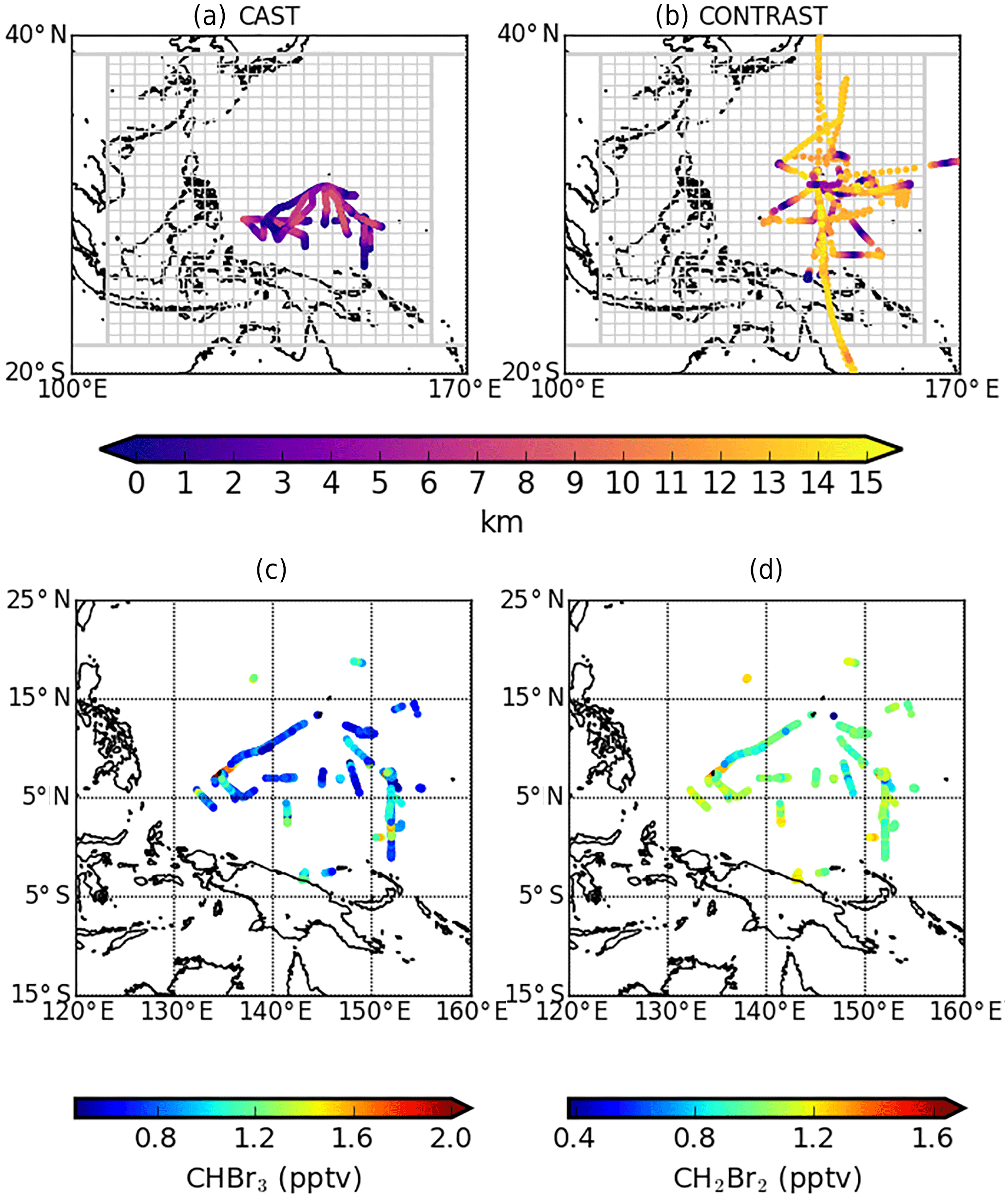
Figure 1 Distributions of data from the (a, c) CAST and (b, d) CONTRAST aircraft campaigns during January and February 2014. Data are described on 2^∘ (latitude) × 2.5^∘ (longitude) GEOS-Chem grid boxes. The top panels show the altitude of data collected by both campaigns. We superimpose the flux inversion domain (grey lattice), consisting of 600 grid boxes between 105 and 165^∘ E and 15^∘ S–25^∘ N, four larger neighbouring regions, and the rest of world. The bottom panels show the distributions of boundary layer (less than 2.5 km) CHBr₃ (pptv) and CH₂Br₂ (pptv) mole fraction data.

To interpret these atmospheric data we use the GEOS-Chem global 3-D atmospheric chemistry transport model (v9.03, http://geos-chem.org; last access: 8 October 2018). We drive the GEOS-Chem model using GEOS-FP meteorological fields, provided by the Global Modeling and Assimilation Office at NASA Goddard, with a horizontal resolution of 2^∘ (latitude) × 2.5^∘ (longitude). We use a tagged version of the model (Butler et al., 2018) in which the atmospheric chemistry is linearized by using pre-computed OH and photolysis loss terms, based on the same GEOS-Chem model but with a more complete description of ${\mathrm{HO}}_x-{\mathrm{NO}}_x-{\mathrm{O}}_x$ and bromine chemistry (Parrelle et al., 2012). Our 3-D OH fields are consistent with the observed methyl chloroform lifetime. We find small (5 %) adjustments to these OH fields do not significantly affect our analysis or conclusions (not shown). For the purpose of our calculations we pre-compute these loss terms every 3 h during the campaign. This tagged modelling approach greatly simplifies the calculation of the Jacobian matrix used by the inverse model to determine surface flux estimates, as described below. We have previously evaluated this version of the model using CHBr₃ and CH₂Br₂ mole fraction data from the NOAA Earth System Research Laboratory (Butler et al., 2018) and have shown a level of agreement with in situ observations that is comparable to the ensemble of models reported by Hossaini et al. (2016a).

We use a priori emissions of CHBr₃ and CH₂Br₂ from the Ordóñez et al. (2012) inventory, which is based on the top-down methodology using aircraft observations from 1996 to 2006. This represents one of three commonly used inventories which were recently evaluated in a multi-model inter-comparison study (Hossaini et al., 2016a). Liang et al. (2010) also employed a top-down methodology to infer CHBr₃ and CH₂Br₂ fluxes, but Ziska et al. (2013) inferred these fluxes from a database of surface ocean observations collected from 1989 to 2011. We find no single inventory is best at reproducing observations of both gases. Ordóñez et al. (2012) assumed a linear relationship between tropical CHBr₃ and CH₂Br₂ emissions and monthly fields of chlorophyll a, a proxy for ocean biological activity, to help fill in the spatial and temporal gaps left by the aircraft data. This approach strongly links the distributions of these two gases in the a priori inventory, an assumption we examine below. We primarily use Ordóñez et al. (2012) but also show the results from other inventories. For our study period, these aggregated regional fluxes are 6.2×10⁸ and $\mathrm{0.9}\pm \mathrm{0.2}\times {\mathrm{10}}^{\mathrm{8}}$ g month⁻¹ for CHBr₃ and CH₂Br₂ over 130–155^∘ E and 0–12^∘ N, respectively.

Figure 1 shows the geographical regions considered in this study. We divide the world into 605 basis functions: (1) a nested domain of 600 grid-scale tagged regions over the tropical western Pacific (105–165^∘ E, 15^∘S–25^∘ N); (2) a lateral boundary of 15^∘ surrounding the nested domain, described by four tagged regions; and (3) the rest of the world. We spin-up the model using a priori inventories (Ordóñez et al., 2012) from 1 July 2013 to 18 January 2014, reducing the impact of initial conditions.

Figure 2 Observed and model mean vertical profiles of (a) CHBr₃ (pptv) and (b) CH₂Br₂ (pptv) from the CAST and CONTRAST campaigns, described on a 1 km resolution grid. Model values have been sampled at the time and location of each observation. Also shown are the model contributions to these gases from within the western Pacific study region, immediately outside the study region and further afield, which we denote as background values. Panel (c) compares CAST and CONTRAST observations of CHBr₃ with GEOS-Chem model simulations using the standard ($\mathrm{2.0}{}^{\circ }\times \mathrm{2.5}{}^{\circ }$) and nested ($\mathrm{0.25}{}^{\circ }\times \mathrm{0.3125}{}^{\circ }$) spatial resolutions from 18 January to 13 February 2014. The two model runs (red and blue lines) use the same emission inventories (Ordóñez et al., 2012). For comparison, we also present posterior model simulations (purple and green lines) based on the a posteriori fluxes inferred from CAST and CONTRAST observations (Fig. 4).

We use the MAP approach to infer CHBr₃ and CH₂Br₂ surface fluxes from atmospheric mole fraction measurements taken by CAST and CONTRAST aircraft campaigns. We infer regional monthly mean surface fluxes, f, of CHBr₃ and CH₂Br₂:

$$\begin{array}{}\text{(1)}& f_p^g\left(x\right)=f_{\mathrm{0}}^g\left(x\right)+\sum _i{\mathit{c}}_i^g{\mathrm{BF}}_i^g\left(x\right),\end{array}$$

where superscript g denotes trace gas, and the subscripts 0 and p denote the a priori and a posteriori state vector, respectively. We describe the regional fluxes as a product of a basis function set BF${}_i^g\left(x\right)$, representing distributions of monthly mean fluxes of the study gases over 605 pre-defined geographic regions (Fig. 1) through the duration of the CAST and CONTRAST aircraft experiments, and scalar coefficients ${\mathit{c}}_i^g$ that are fitted to the data.

We include all the coefficients ${\mathit{c}}_i^g$ for the pre-defined 605 basis functions into the state vector c that describes the CHBr₃ and CH₂Br₂ fluxes, which we fit to the observations. We take into account the uncertainty of the model spin-up by including a scaling factor into the state vector to adjust the background (initial) field, assuming that the model describes the background vertical structure over the study domain. As a result the state vector c has a total of 606 elements. We optimally estimate the state vector c by minimizing the associated cost function J(c):

$$\begin{array}{ll}{\displaystyle }& {\displaystyle }J\left(\mathit{c}\right)={\displaystyle \frac{\mathrm{1}}{\mathrm{2}}}[\mathit{c}-{\mathit{c}}_{\mathrm{0}}{]}^T{\mathbf{B}}^{-\mathrm{1}}[\mathit{c}-{\mathit{c}}_{\mathrm{0}}]+{\displaystyle \frac{\mathrm{1}}{\mathrm{2}}}{\left(y_{\mathrm{obs}}-H\left(\mathit{c}\right)\right)}^T\\ \text{(2)}& {\displaystyle }& {\displaystyle }{\mathbf{R}}^{-\mathrm{1}}\left(y_{\mathrm{obs}}-H\left(\mathit{c}\right)\right),\end{array}$$

where the superscripts T and −1 denote the matrix transpose and inverse operations, respectively; c₀ represents the a priori estimates; and B represents the a priori error covariance matrix. The measurement vector, including the CAST and CONTRAST CHBr₃ and CH₂Br₂ mole fraction data, is denoted by y_obs, and R is the measurement error covariance matrix. The forward model H projects the state vector (scalar coefficients) into observation space (3-D mole fractions), and includes the GEOS-Chem atmospheric chemistry and transport model that is sampled at the time and location of each observation.

We assume a 60 % uncertainty for fluxes within the nested domain and a 50 % uncertainty for fluxes in the lateral boundary and the rest of the world regions, guided by the discrepancy between the top-down and bottom-up inventories and their limited spatial and temporal variation. We also assume that the a priori errors within the nested domain are correlated over a distance of 400 km, corresponding to approximately the width of two adjacent grid boxes. We assume the initial conditions for the mole fractions have a 30 % uncertainty. We assume individual observations of CHBr₃ and CH₂Br₂ have errors of 20 % and 10 %, respectively, and are uncorrelated. These conservative values are guided by an analysis of data collected from different instruments during CAST and CONTRAST (Andrews et al., 2016). We assume that the observation error covariance R is diagonal, which also includes model error, such as the representation error and the errors in modelling atmospheric transport and chemistry processes, with an assumed value of 20 %. Our results over the geographical regions with dense observation coverage are insensitive to different assumptions about a priori uncertainty and observation errors. For example, our changing the a priori emission uncertainty by ±20 % results in changes in the aggregated a posteriori CHBr₃ emission (130–155^∘ E and 0–12^∘ N) of typically less than 10 %.

The Jacobian matrix describes the sensitivity of atmospheric CHBr₃ and CH₂Br₂ CAST and CONTRAST measurements to changes in geographical surface emissions and the initial value on 18 January 2014. We construct it by scaling the tagged tracers originating from a specific geographical region by surface fluxes from that region.

To avoid negative flux estimates due to, for example, an uneven distribution of observations we use value-dependent a priori uncertainties for grid point flux estimates. We assume a functional form for the uncertainty of the flux coefficient c_i (Eq. 1):

$$\begin{array}{}\text{(3)}& \mathit{\sigma }\left(c_i\right)=\left\{\begin{array}{l}\mathrm{0.8},c_i>-\mathrm{0.6}\\ \mathrm{0.8}-\mathrm{2}\left(-\mathrm{0.6}-c_i\right)e^{k\left(\mathrm{1.0}+c_i\right)},c_i<-\mathrm{0.6},\end{array}\right.\end{array}$$

where k (=3) is a pre-chosen factor that defines the gradient of the uncertainty with respect to the change of c_i. Using this approach, the a priori uncertainty decreases rapidly towards zero when c_i becomes smaller than −0.6 (i.e. when the flux estimate is smaller than 40 % of the a priori). We find that using different parameters (e.g. changing the threshold from −0.6 to −0.8) does not significantly change our flux estimates.

3 Results

3.1 Forward model analysis

Figure 2 shows that the model driven by emissions from Ordóñez et al. (2012) overestimates the CHBr₃ concentrations by 0.1–0.7 pptv at altitudes from 0.5 to 12.5 km, with the largest values near the surface that reflects errors in a priori ocean fluxes (Hossaini et al., 2016a; Butler et al., 2018). The model has reasonable skill at reproducing the mean observed vertical gradient (r=0.62) but has a positive model bias of 0.46±0.39 pptv. We find that vertical variations in CHBr₃ are determined approximately equally by sources over the western Pacific study region (Fig. 1) and by sources immediately outside of the nested domain and further afield (Butler et al., 2018). These contributions show different vertical structures. The contribution from fresher sources over the western Pacific has a steeper atmospheric lapse rate from the boundary layer to the free troposphere than the air masses from neighbouring regions. Both contributions are approximately uniform above the free troposphere, with the exception of a peak at 10–12 km from the air being transported into the nested domain (Butler et al., 2018). These differences in vertical structure help the inversion system identify the origin of CHBr₃ at different vertical levels.

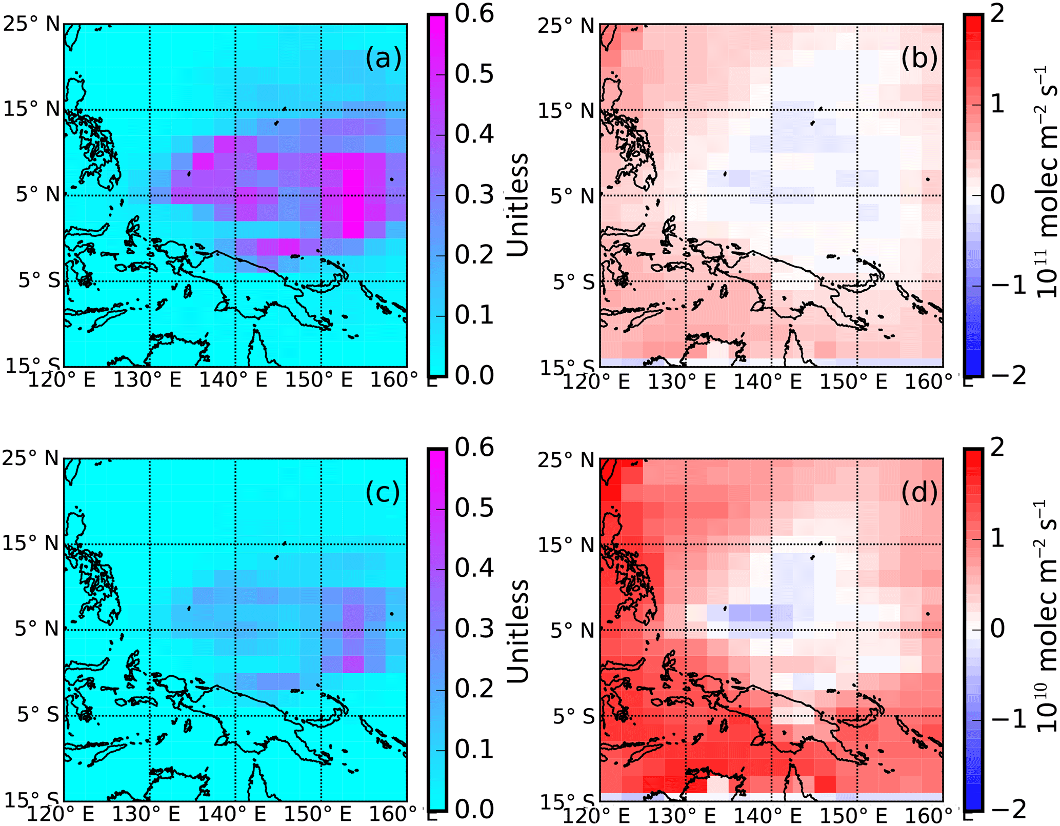
Figure 3 Simulated error reductions (unitless) and a posteriori flux error distributions of CHBr₃ (panels a and b) and CH₂Br₂ (panels c and d) based on the theoretical potential to recover true fluxes using the time and location of CAST and CONTRAST data.

The model reproduces some of the observed CH₂Br₂ variation (r=0.38) but with a small mean bias (0.01 ± 0.14 pptv). Figure 2 shows that the CH₂Br₂ source outside the nested domain represents more than 60 % (0.7–0.9 pptv) of the values sampled over the western Pacific and is almost invariant with altitude. This is due to weaker surface emissions over the western Pacific and the longer atmospheric lifetime of CH₂Br₂ compared to CHBr₃. Ocean emissions from the western Pacific and from the immediate neighbouring regions each contribute only 0.1–0.3 pptv to CH₂Br₂. This highlights the difficulties of inferring ocean fluxes of CH₂Br₂ only using atmospheric CH₂Br₂ data collected over the western Pacific and considering this region in isolation.

To examine model transport errors associated with using a relatively coarse model spatial resolution ($\mathrm{2}{}^{\circ }\times \mathrm{2.5}{}^{\circ }$), we ran a short, high-resolution ($\mathrm{0.25}{}^{\circ }\times \mathrm{0.3125}{}^{\circ }$) simulation of CHBr₃ over a limited spatial domain centred on the western Pacific and compared that against the CAST and CONTRAST data. We acknowledge that we could still miss rapid, sub-grid scale convective events using this model that has a factor of 8 improvement in spatial resolution. However, we find that differences between the two model runs are much smaller than the differences between the individual model runs and the observations (Fig. 2). Figure 2 also shows that the global and nested GEOS-Chem simulations of CHBr₃ and CH₂Br₂ mole fractions, corresponding to our a posteriori flux estimates (Fig. 4), are more consistent with the observations than those from a priori fluxes. This result demonstrates that the a priori model bias can be explained by, in principle, errors in ocean sources.

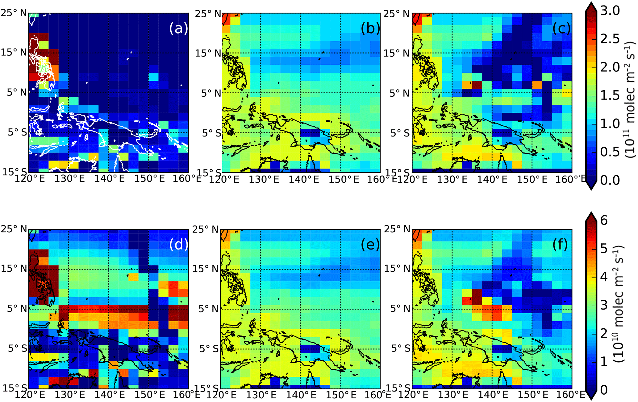
Figure 4 A priori and a posteriori surface fluxes of (top panels) CHBr₃ (10¹¹ mol m⁻² s⁻¹) and (bottom panels) CH₂Br₂ (10¹⁰ mol m⁻² s⁻¹) over the western Pacific study region. Panels (a) and (d) show the a priori fluxes we use in our MAP inversion (Ordóñez et al., 2012); panels (b) and (e) show alternative bottom-up CHBr₃ and CH₂Br₂ emission inventories (Ziska et al., 2013); and panels (c) and (f) show our a posteriori flux estimates inferred from CAST and CONTRAST data.

3.2 Closed-loop numerical experiments

In the absence of independent observations to evaluate our a posteriori ocean fluxes we use closed-loop numerical experiments to understand what we can theoretically achieve from CAST and CONTRAST data, accounting for a realistic description of model and measurement errors. These calculations, often called observing system simulation experiments (OSSEs), provide an upper boundary on the ability of available data to infer the true state.

First, we generate synthetic observations at the time and location of the CAST and CONTRAST data by sampling 3-D model fields of CHBr₃ and CH₂Br₂ mole fractions driven by the a priori inventories, which we regard as the “true” emissions. We consider these sample mole fraction values as the instrument observation after we superimpose instrument (unbiased) noise informed by realistic observation uncertainty. Second, we enlarge the (true) a priori emissions to generate the a priori estimate for the OSSEs: by 50 % for emissions over the western Pacific and by 30 % for emissions from the neighbouring region. The resulting atmospheric mole fractions represent our model a priori concentrations. With perfect coverage of the atmosphere with perfect data (i.e. infinitesimal noise levels), fitting model emissions to the true observations would result in estimating the true ocean emissions. We describe our results as the difference between the a posteriori and true fluxes using a metric (Palmer et al., 2000; Feng et al., 2009) that describes the error reduction g = $\mathrm{1}-{\mathit{\sigma }}_a/{\mathit{\sigma }}_f$, where σ_a and σ_f denote the a posteriori and a priori uncertainties, respectively, ignoring the correlation between state vector elements. The closer the value of g is to unity, the larger the reduction in uncertainty.

Figure 3 shows that the CAST and CONTRAST CH₂Br₂ and CHBr₃ measurements can reproduce the true fluxes, mainly between 130–155^∘ E and 3^∘ S–15^∘ N, by reducing the inflated a priori flux estimate. A posteriori fluxes in several grid boxes are lower than the true value, which is a result of regions overcompensating for other regions that have insufficient data to estimate their emissions. Regions influenced with fewer measurements (Fig. 1) generally have smaller reductions in error, as expected. The error reductions for CHBr₃ range from 0.1 to 0.6 over the study domain, reflecting the widespread sensitivity of the CAST and CONTRAST observations to emissions from the tropical western Pacific region. The mean and median a posteriori fluxes are approximately a factor of 3 closer than the a priori to the true fluxes, with a 40 % improvement in the uncertainties. In contrast, for CH₂Br₂, the error reduction is much smaller, with values greater than 0.3 only over a small geographical region where the data density is greatest. There is a factor of 2 improvement in the discrepancy of the fluxes with the true emissions, and a 30 % improvement in the uncertainties. This large improvement in the knowledge of flux estimates is partly due to our simple description of the difference between the true and a priori field.

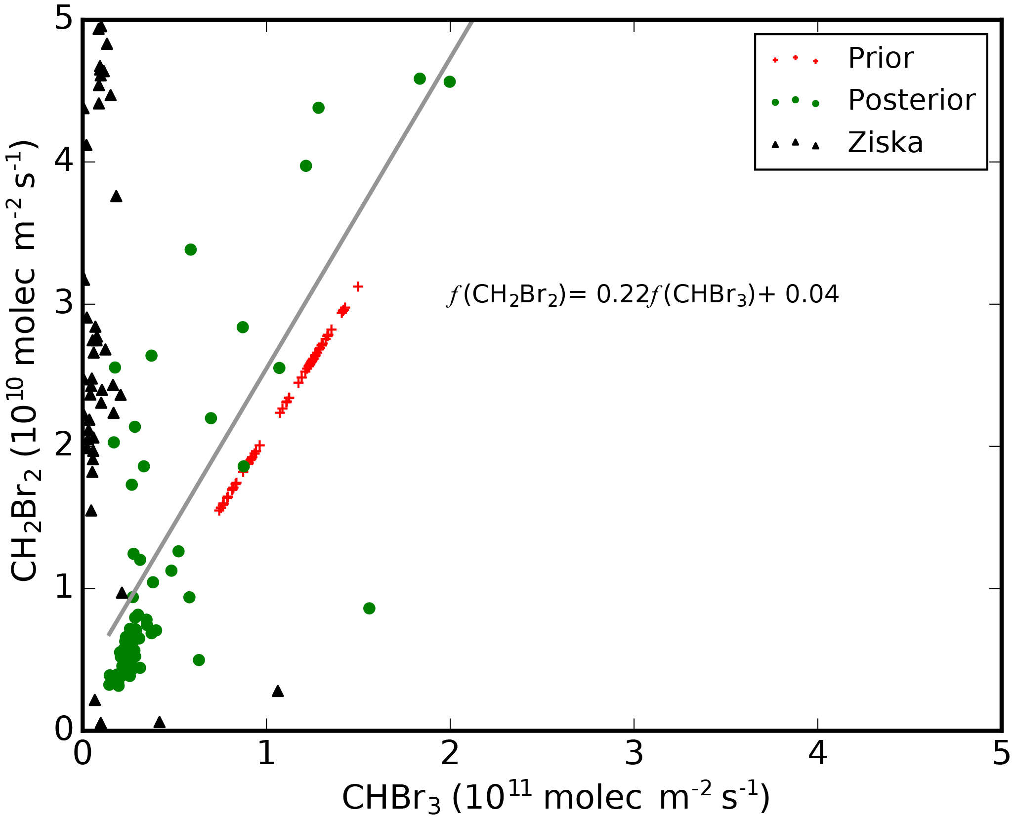
Figure 5 Scatterplot between CHBr₃ and CH₂Br₂ fluxes described on 2^∘ (latitude) × 2.5^∘ (longitude) grid boxes over the main study region (130–155^∘ E and 0–12^∘ N, Fig. 1). Red crosses denote values from Ordóñez et al. (2012), which we use for our a priori; black triangles denote values from an alternative bottom-up inventory (Ziska et al., 2013); and green circles denote our a posteriori values. A posteriori fluxes of CHBr₃ and CH₂Br₂ have a Pearson correlation of 0.86, and the best-fit linear model for the a posteriori fluxes is shown inset.

3.3 Ocean emissions of CHBr₃ and CH₂Br₂ inferred from CAST and CONTRAST data

We now examine the fluxes inferred from the CAST and CONTRAST measurements. Figure 4 shows elevated a posteriori CHBr₃ emissions surrounding small islands north of the tropics, such as Palau (7.4^∘ N, 134.5^∘ E) and Chuuk (7^∘25^′ N, 151^∘47^′ E). However, we find that emissions surrounding Guam (13.5^∘ N, 144.8^∘ E) are not significantly different from the adjacent open ocean. This reflects the distribution of boundary layer measurements (altitudes <2.5 km) of CHBr₃ observed during CAST and CONTRAST flights (Fig. 1). We find that through sensitivity experiments (described below), the a posteriori emissions are inferred by data and not via spatial correlations in the a priori emission inventory. Our a posteriori CHBr₃ emissions are generally higher than the bottom-up estimates from Ziska et al. (2013), particularly over the north of tropics.

We find that our a posteriori CH₂Br₂ emission estimates are lower than the a priori estimates over open oceans north of 5^∘ N. We also find elevated fluxes around islands and parts of open oceans south of 5^∘ N. Similar to CHBr₃, these elevated fluxes coincide with large boundary layer measurements of CH₂Br₂ from CAST and CONTRAST.

Over the study domain (130–155^∘ E and 0–12^∘ N) our a posteriori fluxes are $\mathrm{3.6}\pm \mathrm{0.3}\times {\mathrm{10}}^{\mathrm{8}}$ and $\mathrm{0.7}\pm \mathrm{0.1}\times {\mathrm{10}}^{\mathrm{8}}$ g month⁻¹ for CHBr₃ and CH₂Br₂, respectively. These represent reductions of 40 % and 20 % relative to the a priori values, respectively. We find that our flux estimates are largely insensitive to small changes in the assumed observation and a priori errors. The corresponding a posteriori mole fractions of CHBr₃ and CH₂Br₂ (not shown) have smaller mean biases ($-\mathrm{0.03}\pm \mathrm{0.22}$ pptv, $-\mathrm{0.1}\pm \mathrm{0.11}$ pptv) and more improved correlations (r=0.74, r=0.56) than the a priori values compared to the observations. The small negative model bias of −0.03 pptv in our a posteriori model simulation mainly reflects values in the upper troposphere (Fig. 2), where measurements are less sensitive to local surface fluxes.

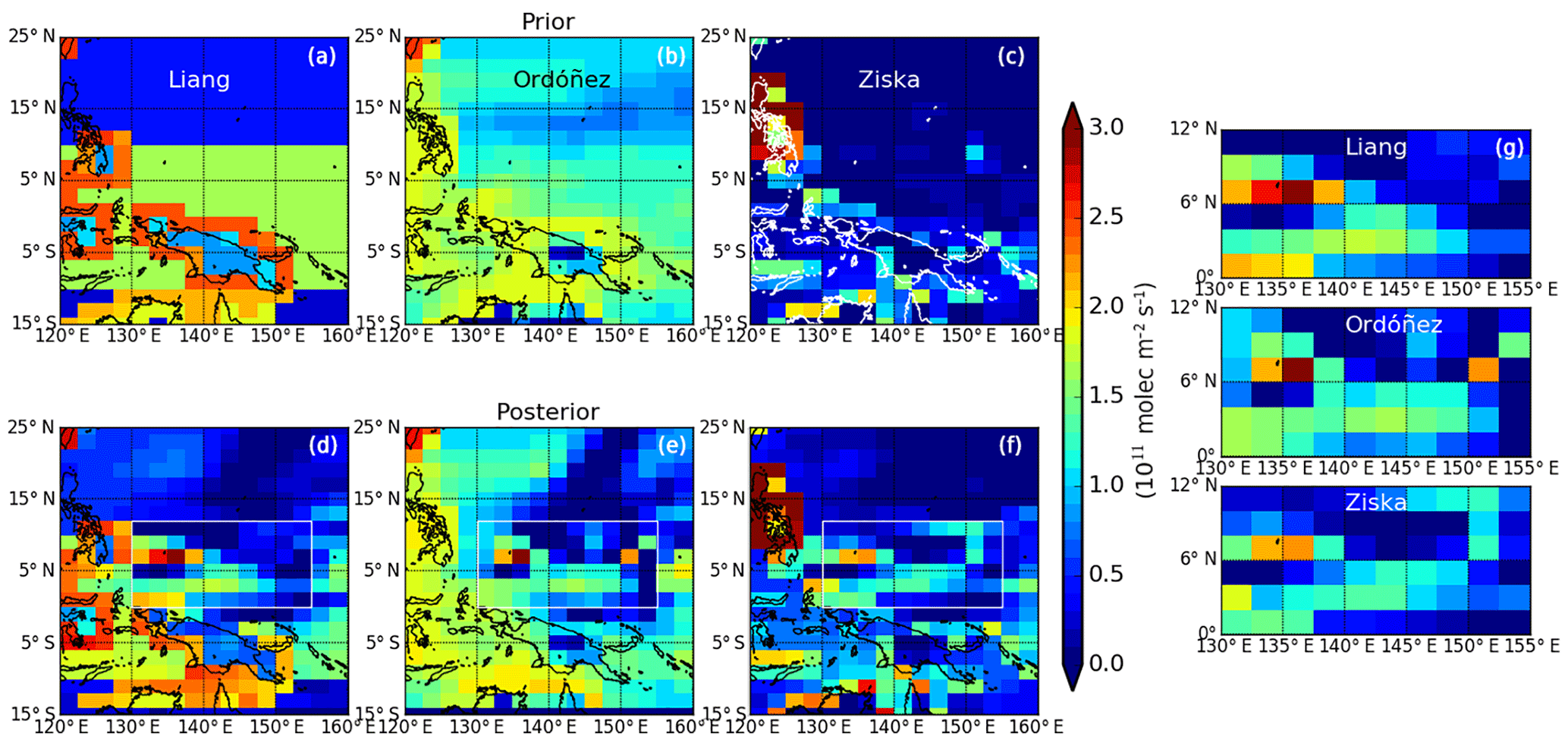
Figure 6 A priori (a) and a posteriori (d) CHBr₃ flux estimates (10¹¹ mol m⁻² s⁻¹) over the study region. The three a priori inventories include Liang et al. (2010), Ordóñez et al. (2012), and. Ziska et al. (2013). The right panel is focused on the geographical region 130–155^∘ E and 0–12^∘ N, where CAST and CONTRAST data density was highest.

This model bias may reflect unaccounted atmospheric model transport error, particularly because we use a relatively coarse atmospheric transport compared to the data resolution. Previous studies have highlighted similar issues (e.g. Russo et al., 2015). Figure 3 shows, however, that CAST and CONTRAST data can only reduce flux uncertainties by about 10 %–60 % over the study regions at this coarse model resolution, limited by the density and coverage of the available data. Using a consistent model simulation but run at a higher spatial resolution ($\mathrm{0.25}{}^{\circ }\times \mathrm{0.3125}{}^{\circ }$) we find insignificant improvement in model performance (Fig. 2). This provides some evidence that our a posteriori emission estimates are robust against the resolution of the meteorological input data. We also find that using this high-resolution model does not significantly reduce the small bias above 8 km. This may point to a small offset between CAST (mostly at lower altitudes <8 km) and CONTRAST measurements (more at higher altitudes) (Andrews et al., 2016). Systematic errors between CAST and CONTRAST data are difficult to fully quantify, but any possible small offset between CAST and CONTRAST data is unlikely to affect our results significantly. Our sensitivity experiments (not shown), in which we introduce a bias between CONTRAST and CAST data that we infer in our inversion, show similar results to our control experiment configuration.

The spatial gradient we find in our a posteriori CHBr₃ emissions between the coasts of Palau and Chuuk and the surrounding open oceans is not present in our a priori emission inventory (Ordóñez et al., 2012). It is, however, qualitatively consistent with observations (e.g. O'Brien et al., 2009; Quack et al., 2007) and bottom-up estimates (e.g. Ziska et al., 2013; Stemmler et al., 2015). These elevated coastal emissions also improve the fit to CAST and CONTRAST observations particularly between 6 and 10 km. Figure 4 shows that the spatial distribution of a priori and a posteriori CH₂Br₂ emissions from the open ocean is different from the climatological bottom-up emissions (Ziska et al., 2013), particularly south of 5^∘ N. This is surprising because studies have shown that tropical ocean emissions of CH₂Br₂ are correlated with the distribution of chlorophyll a (e.g. Liu et al., 2013), but differences may reflect inter-annual changes in ocean biology (e.g. Racault et al., 2017).

Figure 5 shows the a priori and a posteriori CHBr₃ : CH₂Br₂ flux ratios. The top down inventory of Ordóñez et al. (2012) uses a linear model to describe emissions from these two gases, but the bottom-up inventory of Ziska et al. (2013) constructs the emissions of these two gases independently using a database of ocean observations. This discrepancy between the two inventories is why we chose not to exploit this linear relationship in our MAP inversion. Our a posteriori emissions for CHBr₃ and CH₂Br₂ appear to be linearly related at low emissions, but larger values appear to follow a more complicated relationship, which may reflect differences in the responsible ocean biological processes. This is supported by field data (Leedham et al., 2013) that showed CHBr₃ : CH₂Br₂ ratios vary between different species.

To examine the sensitivity of our results to the a priori inventories, we use the same MAP approach to infer the CHBr₃ flux from CAST and CONTRAST measurements for three different prior inventories (Fig. 6): (a) Ziska et al. (2013); (b) Liang et al. (2010); and (c) Ordóñez et al. (2012). For simplicity, we assume the same a priori error covariance for the 600 grid boxes over the tropical western Pacific (Fig. 1) when the three different a priori inventories are used. Figure 6 shows that despite a large a priori discrepancy, the three sets of a posteriori flux estimates (Fig. 6) show similar features over our study domain between 130 and 155^∘ E and 0–12^∘ N (as denoted by white rectangles). Despite there being a large discrepancy between CHBr₃ ocean emission estimates over our study region from Ziska et al. (2013) (0.73×10⁸ g month⁻¹) and Liang et al. (2010) (6.9×10⁸ g month⁻¹) inventories, we infer similar aggregated a posteriori emissions of 3.0×10⁸ and 3.5×10⁸ g month⁻¹ from Ziska et al. (2013) and Liang et al. (2010), respectively. This suggests that the choice of a priori plays only a small role in determining the a posteriori solution. These a posteriori estimates are also comparable with fluxes from our control experiment ($\mathrm{3.6}\pm \mathrm{0.3}\times {\mathrm{10}}^{\mathrm{8}}$ g month⁻¹) that uses a priori emissions from Ordóñez et al. (2012). We find that outside our study domain, the discrepancies in posterior fluxes are still very large, in particular over coastal regions, due to the limited observation coverage by CAST and CONTRAST experiments.

4 Summary and concluding remarks

Very short-lived brominated gases have predominately natural sources, and therefore cannot be regulated by international agreements (Oman et al., 2016; Butler et al., 2007). Current understanding of these natural sources is poor due to the infrequent and incomplete measurements of ocean fluxes that vary in space and time. Past studies have relied on developing bottom up inventories using a database of ship-borne measurements or a heuristic top down method that adjusted a priori emissions to match tropospheric and lower stratospheric measurements of a range of gases, including of CHBr₃ and CH₂Br₂. As a consequence of the uncertainties associated with the modelling and data, the resulting inventories adopt simple distributions and are not necessarily consistent with each other on regional spatial scales.

Here, we used an a priori inventory to reproduce observed atmospheric boundary layer variations of CHBr₃ and CH₂Br₂ over a small geographical region encompassing Guam, Palau and Chuuk over the western Pacific. The measurements were collected as part of the CAST and CONTRAST aircraft campaigns during January and February 2014. We use the GEOS-Chem atmospheric chemistry model to relate the a priori emissions to the atmospheric concentrations, and develop a MAP inverse model to infer the ocean fluxes that correspond with the aircraft measurements.

First, using a small number of closed-loop numerical experiments we showed that the aircraft data could in theory, using assumptions about their uncertainties, improve knowledge of ocean fluxes. Improvements in knowledge are generally related to the density of measurements, as expected.

Using the aircraft data we find substantial spatial variations in fluxes of both gases that differ significantly from the a priori inventory. We find that aggregated regional a posteriori fluxes of CHBr₃ ($\mathrm{3.6}\pm \mathrm{0.3}\times {\mathrm{10}}^{\mathrm{8}}$ g month⁻¹) and CH₂Br₂ ($\mathrm{0.7}\pm \mathrm{0.1}\times {\mathrm{10}}^{\mathrm{8}}$ g month⁻¹) are 40 % and 20 % lower than the a priori fluxes over the main study domain (130–155^∘ E and 0–12^∘ N). Using the model we find that observed variations of CHBr₃ are determined mainly by the open ocean while CH₂Br₂ has a large influence from outside the immediate study region. A posteriori fluxes significantly improve the mean observed vertical gradient of both gases, particularly in the free troposphere. We also find no evidence to suggest a robust linear relationship between the emissions of these two gases over the study region, unlike one of the top-down a priori inventories. This discrepancy may reflect differences in the analysis of data over different spatial scales or the construction of the a priori inventory using data in the free and upper troposphere, where observed air masses originating from disparate surface sources have time to mix.

The MAP approach we used fits a posteriori fluxes to minimize the discrepancy between model and observed atmospheric mole fractions. Any discrepancy in atmospheric data may result from errors in surface fluxes (emissions minus uptake), atmospheric chemistry and atmospheric transport. Where observation coverage is denser, our inversion results are less sensitive to the assumed a priori inventories, as expected. The next most likely source of error is atmospheric transport, particularly sub-grid scale vertical mixing. Sensitivity tests that crudely account for model errors suggest that the a posteriori fluxes are robust.

Our paper highlights the value of using atmospheric data to improve the magnitude and distribution of ocean emissions of halogenated gases but also shows some of the difficulties associated with interpreting these data even with the aid of an atmospheric transport model. Future scientific progress in quantitatively understanding the role of natural emissions of halogens in the catalytic destruction of stratospheric ozone is hampered by the lack of available observations.