the Creative Commons Attribution 4.0 License.
the Creative Commons Attribution 4.0 License.
 | 01 Oct 2018
Characterization of trace gas emissions at an intermediate port
Li Li
Keane Tobin
Morgan Mitchell
Growing ship traffic in Atlantic Canada strengthens the local economy but also plays an important role in greenhouse gas and air pollutant emissions in this coastal environment. A mobile open-path Fourier transform infrared (OP-FTIR; acronyms defined in Appendix A) spectrometer was set up in Halifax Harbour (Nova Scotia, Canada), an intermediate harbour integrated into the downtown core, to measure trace gas concentrations in the vicinity of marine vessels, in some cases with direct or near-direct marine combustion plume intercepts. This is the first application of the OP-FTIR measurement technique to real-time, spectroscopic measurements of CO2, CO, O3, NO2, NH3, CH3OH, HCHO, CH4 and N2O in the vicinity of harbour emissions originating from a variety of marine vessels, and the first measurement of shipping emissions in the ambient environment along the eastern seaboard of North America outside of the Gulf Coast. The spectrometer, its active mid-IR source and its detector were located on shore while the passive retroreflector was on a nearby island, yielding a 455 m open path over the ocean (910 m two-way). Atmospheric absorption spectra were recorded during day, night, sunny, cloudy and substantially foggy or precipitating conditions, with a temporal resolution of 1 min or better. A weather station was co-located with the retroreflector to aid in the processing of absorption spectra and the interpretation of results, while a webcam recorded images of the harbour once per minute. Trace gas concentrations were retrieved from spectra by the MALT non-linear least squares iterative fitting routine. During field measurements (7 days in July–August 2016; 12 days in January 2017) AIS information on nearby ship activity was manually collected from a commercial website and used to calculate emission rates of shipping combustion products (CO2, CO, NOx, HC, SO2), which were then linked to measured concentration variations using ship position and wind information. During periods of low wind speed we observed extended (∼9 h) emission accumulations combined with near-complete O3 titration, both in winter and in summer. Our results compare well with a NAPS monitoring station ∼1 km away, pointing to the extended spatial scale of this effect, commonly found in much larger European shipping channels. We calculated total marine sector emissions in Halifax Harbour based on a complete AIS dataset of ship activity during the cruise ship season (May–October 2015) and the remainder of the year (November 2015–April 2016) and found trace gas emissions (tonnes) to be 2.8 % higher on average during the cruise ship season, when passenger ship emissions were found to contribute 18 % of emitted CO2, CO, NOx, SO2 and HC (0.5 % in the off season due to occasional cruise ships arriving, even in April). Similarly, calculated particulate emissions are 4.1 % higher during the cruise ship season, when passenger ship emissions contribute 18 % of the emitted particulate matter (PM) (0.5 % in the off season). Tugs were found to make the biggest contribution to harbour emissions of trace gases in both cruise ship season (23 % NOx, 24 % SO2) and the off season (26 % of both SO2 and NOx), followed by container ships (25 % NOx and SO2 in the off season, 21 % NOx and SO2 in cruise ship season). In the cruise ship season cruise ships were observed to be in third place regarding trace gas emissions, whilst tankers were in third place in the off season, with both being responsible for 18 % of the calculated emissions. While the concentrations of all regulated trace gases measured by OP-FTIR as well as the nearby in situ NAPS sensors were well below maximum hourly permissible levels at all times during the 19-day measurement period, we find that AIS-based shipping emissions of NOx over the course of 1 year are 4.2 times greater than those of a nearby 500 MW stationary source emitter and greater than or comparable to all vehicle NOx emissions in the city. Our findings highlight the need to accurately represent emissions from the shipping and marine sectors at intermediate ports integrated into urban environments. Emissions can be represented as pseudo-stationary and/or pseudo-line sources.
- Article
(10245 KB) - Full-text XML
-
Supplement
(572 KB) - BibTeX
- EndNote


1.1 World shipping trends and emissions regulations
In 2015, seaborne trade is estimated to have accounted for more than 80 % of total world merchandise trade. Seaborne trade volume expanded by 2.1 % in 2015 (3.5 % in 2014) and it continues to grow, albeit not without challenges (UNCTAD, 2016, p. 25). Shipping is also the most efficient transportation mode with the lowest greenhouse gas emissions per tonne of cargo and per kilometre of transport as compared to rail, road and air (Seyler et al., 2017). Between 2007 and 2012 shipping emissions comprised only 2.8 % on average of global CO2-equivalent emissions (incorporating CH4 and N2O) from fossil fuel consumption and cement production (International Maritime Organization, 2015); however, while other land-based sources work to reduce emissions, shipping emissions are projected to increase by between 50 % and 250 % by the year 2050, depending on economic and energy developments, as well as efficiency improvements. The great majority (86 %) of the above-mentioned global emissions come from international shipping and are dominated by container, bulk carrier and tanker emissions from main engine operations (as opposed to auxiliary engines and boilers). Compared to CO2-equivalent emissions, global NOx and SOx emissions from all shipping comprise a higher proportion of anthropogenic sources at 15 % and 13 % (International Maritime Organization, 2015), respectively. The majority of these emissions are again from international shipping and are projected to increase along with CO2, as the shipping sector grows. Individual ship SOx emissions will continue to decline through 2050 due to the IMO International Convention for the Prevention of Pollution from Ships (MARPOL Annex VI) requirements on the FSC in ships sailing globally and within SECAs, which is further explained below and in Appendix A. Emissions of NOx will be modulated by Tier I, II and III controls on ships sailing globally and within NECAs (see below and Appendix A). Notably, if fuels shift to LNG, then methane emissions will increase rapidly (International Maritime Organization, 2015). The recent designation of the North and Baltic seas as NECAs (World Maritime News, 2016) is predicted to lead to a greater shift to LNG in the shipping fleet fuel mix (Jonson et al., 2015).
IMO regulations regarding SOx (and associated particulate matter, PM) emissions in a SECA historically required a reduction of FSC from the global average at the time of the SECA entering into force to 1.5 % (by mass) prior to July 2010, a further reduction to 1.0 % after this date, and a final reduction to 0.1 % after January 2015. The actual historical FSC used in a given shipping area depends on when the relevant SECA began to be enforced. The Baltic and North seas' SECAs began to be enforced in 2006 and 2007, respectively (Jonson et al., 2015), while the North American SECA (including most of the continental US and Canada) began to be enforced in August 2012 (Environment Canada, 2012). Thus, in our study location in Halifax, Canada, the FSC of ships was reduced in August 2012 from an average value below the global FSC limit of 3.5 % (applicable at the time) to 1.0 %, and again in January 2015 from 1.0 % to 0.1 %. The global FSC limit was recently approved to be reduced from 3.5 % to 0.5 % in 2020 (IMO Resolution MEPC.280(70), adopted 28 October 2016).
A similar complexity applies to IMO regulations regarding NOx emissions in NECAs. The North American NECA was fully implemented in August 2012, with the implication that ships constructed after January 2016 have to comply with Tier III controls on NOx emissions for engine power greater than 130 kW. Tier III controls are a function of engine speed (rpm) and lead to 80 % lower NOx emissions as compared to Tier I controls (for ships built after the year 2000 but before 2011) and 75 % lower NOx emissions as compared to Tier II controls (for ships built after 2011 but before 2016). Outside of the North American and Caribbean NECAs Tier I and II controls apply globally, with Tier III controls coming into force in 2021 in the newly designated Baltic Sea and North Sea NECAs. Due to the long lifetime of ships, it will take approximately 30 years before full fleet renewal to Tier III compliance is complete (Jonson et al., 2015).
1.2 Atmospheric chemistry, health and climate impacts of shipping
While shipping consumes only 16 % of the fuel used by the entire transportation sector it produces 9.2 times the NOx of the aviation sector and 80 % of the NOx produced by vehicles (Eyring et al., 2005), primarily due to the high-temperature combustion of diesel engines combined with a lack of strong regulation – until recently. Where NOx, CO and other hydrocarbon ship emissions occur in pristine marine boundary layers, a high ozone production efficiency results in increased background O3 concentrations, increased OH and thereby a reduced methane lifetime. Up to 12 ppbv O3 increases are calculated by Endresen (2003) in a model study in summer in the North Atlantic and North Pacific. In more NOx-polluted regions the relative perturbation to O3 concentrations is smaller but not negligible, i.e., 3–5 ppbv over Nova Scotia in July (Endresen, 2003, their Fig. 10d). The potentially large relative importance of shipping NOx emissions in intermediate ports and urban environments with relatively low background levels of NOx has been noted by Dalsøren et al. (2010), although in their work the effect is most apparent for the Atlantic Canadian port of St. John's, Newfoundland (their Fig. 10), which has one-fourth the population of Halifax and likely even lower background NOx levels. More recently, Aulinger et al. (2016) also found that shipping emissions significantly increased the incidence of daily 8 h maximum O3 exceedances in areas where they comprised a sizeable fraction of emitted NOx. At high NOx concentrations, NOx has a lifetime of hours to days against removal by HNO3 formation and subsequent wet and dry deposition (Endresen, 2003) and via night-time loss pathways that first involve the formation of NO3 then equilibrium with N2O5, followed by its hydrolysis to nitric acid (Vinken et al., 2011).
Shipping also leads to particulate emissions in the form of black carbon (Lack and Corbett, 2012), organic carbon, hydrated sulfates and trace metals (e.g., Celo et al., 2015). These primary particulate emissions are elevated over shipping routes, while secondary aerosols, dominated by the inorganic fraction have a much further spatial reach (e.g., Aksoyoglu et al., 2016). The composition of the secondary inorganic fraction will shift from ammonium sulphate towards ammonium nitrate as shipping sulfur emissions decline, especially in regions with abundant ammonia emissions (Aulinger et al., 2016).
With 70 % of shipping emissions occurring within 400 km of land (Corbett et al., 1999), cardiopulmonary and lung cancer mortality due to primary and secondary shipping emissions of PM2.5 have been estimated at ∼60 000 per year, concentrated in densely populated coastal regions as well as regions downwind of shipping lanes and ports (Corbett et al., 2007). These mortality estimates will be reduced by legislated fuel sulfur content reductions and increased by the growth of the shipping sector and the continued emissions of primary particulates and NOx (leading to nitrogen-based secondary inorganic PM2.5 formation), as well as the formation of other secondary aerosols. A more recent study by Liu et al. (2016) based on higher Asian shipping emissions that are still largely unregulated, AIS-based activity data (see below), expanded causes of death (i.e., respiratory illness), and updated exposure–response functions has produced a similar range of East Asian PM2.5-related mortality (8700–25 500 cases per year) as the earlier work of Corbett (1000–32 000 cases per year in East Asia), with a further 5800–12 000 mortalities due to secondary ozone. In the busy North and Baltic seas, Jonson et al. (2015) estimate 0.1–0.2 years of life lost in areas close to major ship tracks at current emission levels while demonstrating the positive effects of recent and future regulations to curb SOx and NOx emissions. Although shipping-related annual mortality estimates are low in Nova Scotia as a result of the low population density, the concentration of shipping-related PM2.5 estimated by Corbett et al. (2007, their Fig. 1), which determines exposure and risk factors, is as high in Halifax as along other major global shipping routes, i.e., northern Europe, the Mediterranean and East Asia, further motivating the continued study of shipping emissions in this region as the regulations on NOx, SOx and PM emissions evolve in a protracted international legal process.
The primary and secondary perturbations to tropospheric gases and aerosols lead to a small but highly uncertain climate forcing. This is due to both the offsetting warming effects from CO2 emissions and secondary O3, and the indirect aerosol cooling effects and the cooling from CH4 lifetime reduction (Eyring et al., 2007, 2010). While greenhouse gas warming effects are global in nature due to their long lifetimes, direct and indirect aerosol cooling effects are regional (Liu et al., 2016) and expected to decrease as sulfur emissions are reduced under increasingly restrictive legislation.
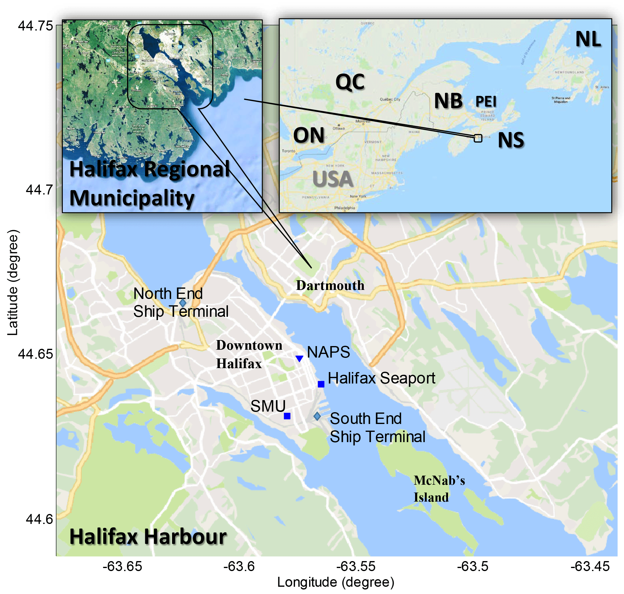
Figure 1Location of Halifax Harbour within the Halifax Regional Municipality and eastern Canada/northeast USA. Also shown is the location of provincial/federal NAPS trace gas and aerosol monitoring, the measurement location (Halifax Seaport) and Saint Mary's University (SMU).
1.3 Shipping in Halifax, Canada
The Port of Halifax (Fig. 1), Nova Scotia, was ranked 24th out of the top 50 NAFTA region container ports, based on container volume, and as such represents an intermediate port environment. It is the fourth largest port in Canada (again measured by container volume) and one of the most important inbound port gateways in North America, connected to more than 150 countries via 18 direct shipping lines. According to the administering Halifax Port Authority (2017), between 2012 and 2016 the total cargo (containerized or otherwise) handled at the port was 8.4 million metric tonnes per year, on average. In 2015/16 the port generated more than 37 000 full-time equivalent jobs (>12 000 in direct port operations) which represents 8.3 % of Nova Scotia's employed labour force, and is responsible for generating USD 3.6 billion in gross economic output (USD 1.9 billion from direct operations, USD 1.7 billion from exports). In addition to providing services for container, bulk, break-bulk, and Ro-Ro cargo ships, the Port of Halifax receives calls from more than 130 cruise ships which carry ∼230 000 visitors to Halifax each year (2012–2016 average). In 2017 cruise ship numbers rose sharply to 177 ships, which carried up to 298 000 passengers (http://cruisehalifax.ca, last access: September 2017). This growth is the result of a broader strategy of continued investment in port facilities to support provincial growth targets for trade activity, tourism and aquaculture exports (Halifax Port Authority, 2017). Unlike many North American ports, the Port of Halifax is fully integrated into the city's urban core, increasing exposure and motivating the present field study as well as future, longer-term measurements of trace gases in Halifax.
1.4 Previous studies of shipping emissions
Shipping emissions have been studied in laboratory test engines (e.g., Petzold et al., 2008; Reda et al., 2014), on-board from auxiliary engines operating at berth (Cooper, 2003), on-board from main engines operating at sea (e.g., Agrawal, 2008a, b; Moldanová et al., 2009; Fu et al., 2013; Celo et al., 2015; Zhang et al., 2016), by intercepting plumes from aircraft (e.g., Sinha et al., 2003; Chen et al., 2005; Lack et al., 2011; Berg et al., 2012; Aliabadi et al., 2016) and from other ships (e.g., Williams et al., 2009; Cappa et al., 2014) as well as by using combined sampling approaches (e.g., Petzold et al., 2008; Murphy et al., 2009). A large number of studies have measured the effects of shipping emissions on air quality from some distance on land, either by in situ (e.g., Lu et al., 2006; Marr et al., 2007; Poplawski et al., 2011; Alföldy et al., 2013; Diesch et al., 2013; Pirjola et al., 2014) or remote sensing techniques (McLaren et al., 2012; Burgard and Bria, 2016; Merico et al., 2016; Seyler et al., 2017). Where gaseous emissions were reported, they were typically of NO, NO2, SO2, CO and total VOCs. All shipping emission studies relating to Canada (Lu et al., 2006; Poplawski et al., 2011; McLaren et al., 2012; Burgard and Bria, 2016) focus on Canada's largest port of Vancouver and cover time periods prior to 2010, when permitted FSC was at the globally applicable maximum of 4.5 % (prior to January 2012) and only Tier I NOx emission controls were applicable to engines built after 2000 (the North American SECA and NECA were not fully implemented until August 2012.) The contribution of shipping emissions to air quality in Halifax has previously been estimated by Hingston (2005) and Phinney et al. (2006). The former was a bottom-up inventory of emissions while the latter was an analysis of NOx and SO2 concentrations measured at the NAPS monitoring site (discussed in detail in Sect. 2.3) under winds prevailing from the marine geographic sector. They estimated SO2 and NOx from shipping to contribute <10 % (Hingston 2005) of emissions but ∼30 % (Phinney et al., 2006) of concentrations in Halifax under the high SOx emissions regime of 2002. Finally, two separate studies that used positive matrix factorization analysis of chemical markers supported by air mass back trajectory calculations and local wind analyses have found that shipping emissions accounted for between 3.4 % of PM2.5 mass (Gibson et al., 2013) and 9.1 % of PM2.5 mass (Jeong et al., 2011) during 45 days and 22 months of continuous field measurements, respectively.
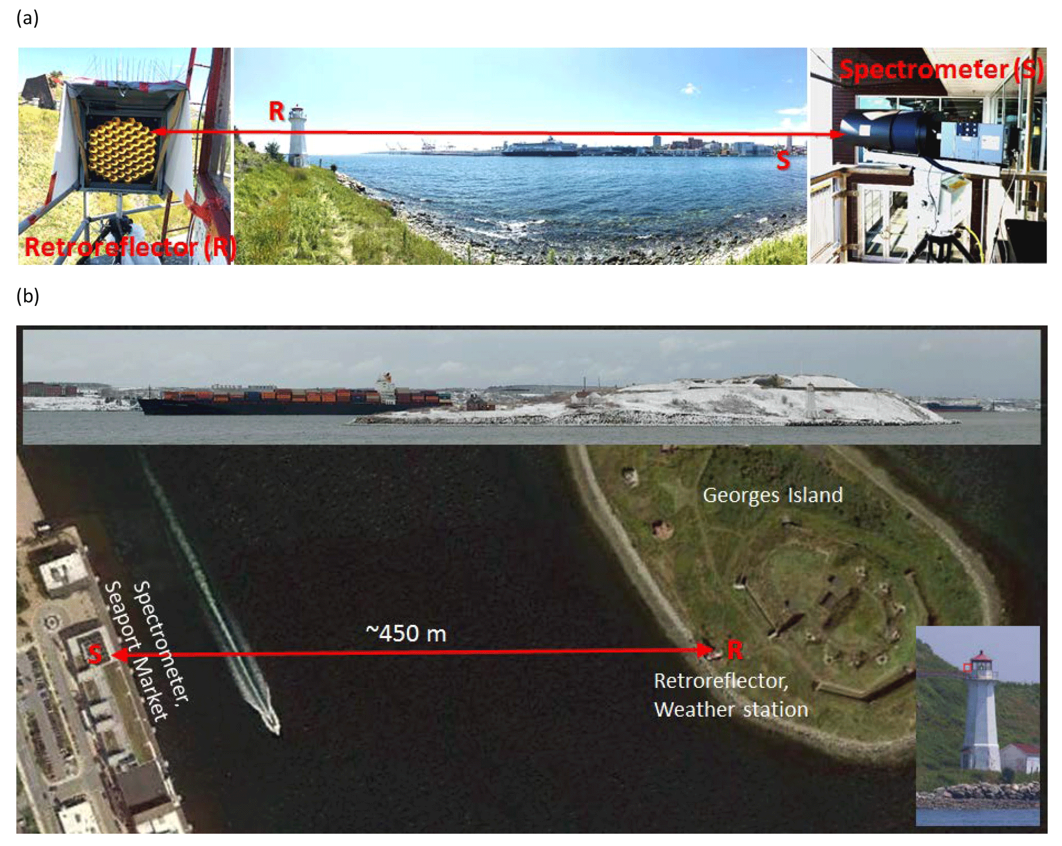
Figure 2OP-FTIR system set-up. (a) Spectrometer location with IR source, FTIR spectrometer, a single transmitting and receiving telescope, and a detector. Retroreflector location on lighthouse catwalk and weather station (not shown). (b) Plan view of measurement geometry with sample speedboat crossing below open path. Top inset: container cargo vessel moving behind the island. Bottom inset: location of retroreflector (uninstalled) marked with red square.
1.5 Aims of this study
The open-path FTIR remote sensing technique has typical detection limits of ∼1–10 ppbv (depending on path length and co-adding time), which is higher than in situ or UV-based remote sensing techniques; however, all trace gases have infrared spectral signatures and many are suitable for quantitative analysis. As such, the first aim of our study was to assess the signatures of individual or blended ship plumes from typical harbour activities in the urban core of Halifax, in concentrations of CO2, CO, O3, NO, NO2, NH3, CH3OH, HCHO, CH4, N2O, SO2, HNO3, HONO, C2H6, C2H4, C2H2 and other VOCs retrieved from infrared spectra recorded in close proximity to ship emissions. Second, we compare our measurements with nearby (∼1 km away) NAPS monitoring station measurements to better understand the effects of in situ vs. open-path sampling geometries, and the spatial extent of the influence of shipping emissions in Halifax Harbour. Third, we estimate the contribution of ship vs. land-based sources to air pollution at an intermediate port with relatively low background NOx concentrations (18 ppb annual average in 2015). The fourth and final aim of our study was to establish a baseline of trace gas concentration measurements as NECA regulations begin to affect an increasing percentage of the fleet, and as shipping activity and shipping fuel mixtures evolve with time. While baselines are recognized as important and necessary in future studies, air monitoring in Halifax is currently limited to the NAPS program; moreover, research in North America has focused on the West Coast and the Gulf Coast, making eastern seaboard measurements highly relevant.
2.1 Open-path FTIR measurements of trace gas concentrations
A wide variety of trace gas species can be measured with high temporal resolution during both day and night using the open-path FTIR spectroscopic technique. Measurements are also possible during significant fog and precipitation events due to the weaker scattering of infrared radiation by the condensed phase (fog and rain droplets) in the beam. The monostatic OP-FTIR configuration (co-located source and detector) has recently been applied to measure biomass burning emission factors (e.g., Paton-Walsh et al., 2014; Akagi et al., 2014), agricultural emissions (e.g., Flesch et al., 2016, 2017) and vehicle emissions (e.g., You et al., 2017). Over the course of 7 days in July and August (2016) and 12 days in January (2017) a mobile OP-FTIR spectrometer was set up between Halifax Harbour and George's Island lighthouse to detect trace gas concentrations in the vicinity of marine vessel emissions, with the possibility of direct or near-direct plume intercepts. To the best of our knowledge, this is the first application of this technique to trace gas measurements in a shipping environment. Figure 2 shows the geometry of the OP-FTIR system set-up during the campaign in Halifax Harbour. The components comprise Bruker's “Open Path System” arranged in a monostatic configuration (Jarvis, 2003). The active broadband IR source is modulated by a low-resolution Fourier transform spectrometer and passed to a modified transmitting 12 telescope, also serving as a receiving unit. Collimated radiation returning from the retroreflecting cube corner array is focused on a broadband IR detector, in our system a mercury–cadmium–telluride element responsive between 700 and 6000 cm−1 with Stirling cycle cryocooling. A significant advantage of this configuration is that only the FTS-modulated returning radiation is detected, while unmodulated emitted atmospheric radiation in the wavelength range of the detector is ignored as DC signal by the signal processing electronics.
The separation between the telescope and retroreflector must be large enough that sufficient absorption for detection can be achieved, which is different for each target trace gas in accordance with its concentration and absorption cross section. In practice, one-way open paths greater than ∼500 m lead to greatly diminishing signal returns due to imperfect beam collimation, which in our system leads to overfilling the retroreflector array at and beyond separations of ∼300 m. Moreover, with increasing atmospheric path, interfering absorption from water vapour and carbon dioxide increases and strongly overlaps target gas features. The 910 m optical path length (455 m physical separation) used in our study was dictated by the separation between the mainland and George's Island. The measurement path is spatially well defined in the planetary boundary layer and bridges the spatial scales of in situ point measurements and newer space-based satellite measurements.
We used the maximum spectral resolution of our system (0.5 cm−1), as is appropriate for sampling strongly Lorentz-broadened rotational–vibrational gas absorption features at 1 atm. To improve the SNR, we co-added 240 interferograms operating at 4 Hz to produce a single spectrum once per minute. In an attempt to resolve finer plumes of ships moving directly within our line of sight we reduced the sampling interval to 10 s (40 co-added interferograms) in most of our summer measurements, which reduced the SNR by .
Spectral acquisition was carried out with Bruker's proprietary software (OPUS RS) while trace gas retrievals were performed with a NLLS iterative fitting routine (Griffith et al., 2012) using the MALT forward model (Griffith, 1996) and MATLAB® processing tools developed in house. The NLLS retrieval derives trace gas concentrations from transmittance spectra through an iterative fitting process that minimizes a least squares cost function between measured and calculated spectra. This process takes into account target and interfering gas absorptions, spectrum continuum shape, and instrumental lineshape parameters describing line broadening and asymmetry under both ideal (finite optical path difference and field of view, apodization) and real (wavenumber shift, phase error, effective apodization) spectrometer conditions (Griffith, 1996). The forward spectral model does not assume linearity in Beer's law for absorbance vs. concentration, meaning that both weakly and strongly absorbing spectral features can be used in the analysis. Forward modelled spectra were calculated based on temperature- and pressure-dependent line-by-line absorption coefficients from the HITRAN 2012 database (Rothman et al., 2013) and real-time temperatures and pressures measured at the retroreflector end of the open path using a commercial weather station (Davis, Vantage Pro 2), which also recorded solar and UV radiation, wind speed and wind direction.
Table 1Spectroscopic retrieval parameters and detection limits for gases measured with an optical path of 913.7 m.
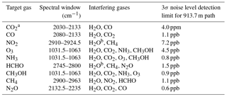
a CO2 residual de-weighted from 2074 to 2080 in cost function to skip known line mixing fitting error. b The HITRAN 2004 database was used for water in these specific retrievals, otherwise HITRAN 2012 was used.
The inverse result is not unique because of noise in the spectra and represents the most probable set of trace gas concentrations, continuum coefficients and instrumental parameters given the measured spectrum. The full set of retrieval parameters used is shown in Table 1. Instrumental parameters of resolution and field-of-view were fixed but instrumental parameters of wavenumber shift, phase error and effective apodization were retrieved. Spectral continuum curvature was retrieved as a slope and intercept only but spectra were divided by the short-path background spectrum to remove complex continuum features that cannot be modelled by polynomial functions with good numerical stability. Retrieval parameters were optimized to result in minimal spectral fit residuals (RMS residuals typically ∼0.5 %), unbiased trace gas concentrations and variations in time that are uncorrelated with concentrations of other gases. Although FTIR retrievals are precise, the accuracy has been conservatively estimated as “well below 10 %” by Smith et al. (2011) for species with strong absorption features (CO2, CH4, CO), mainly driven by the accuracy of spectral parameters, the MALT forward model, spectrometer alignment, pressure and temperature representative of the path average and retrieved parameter errors. For species with weak absorption features or subject to interference from water vapour these errors may be higher.
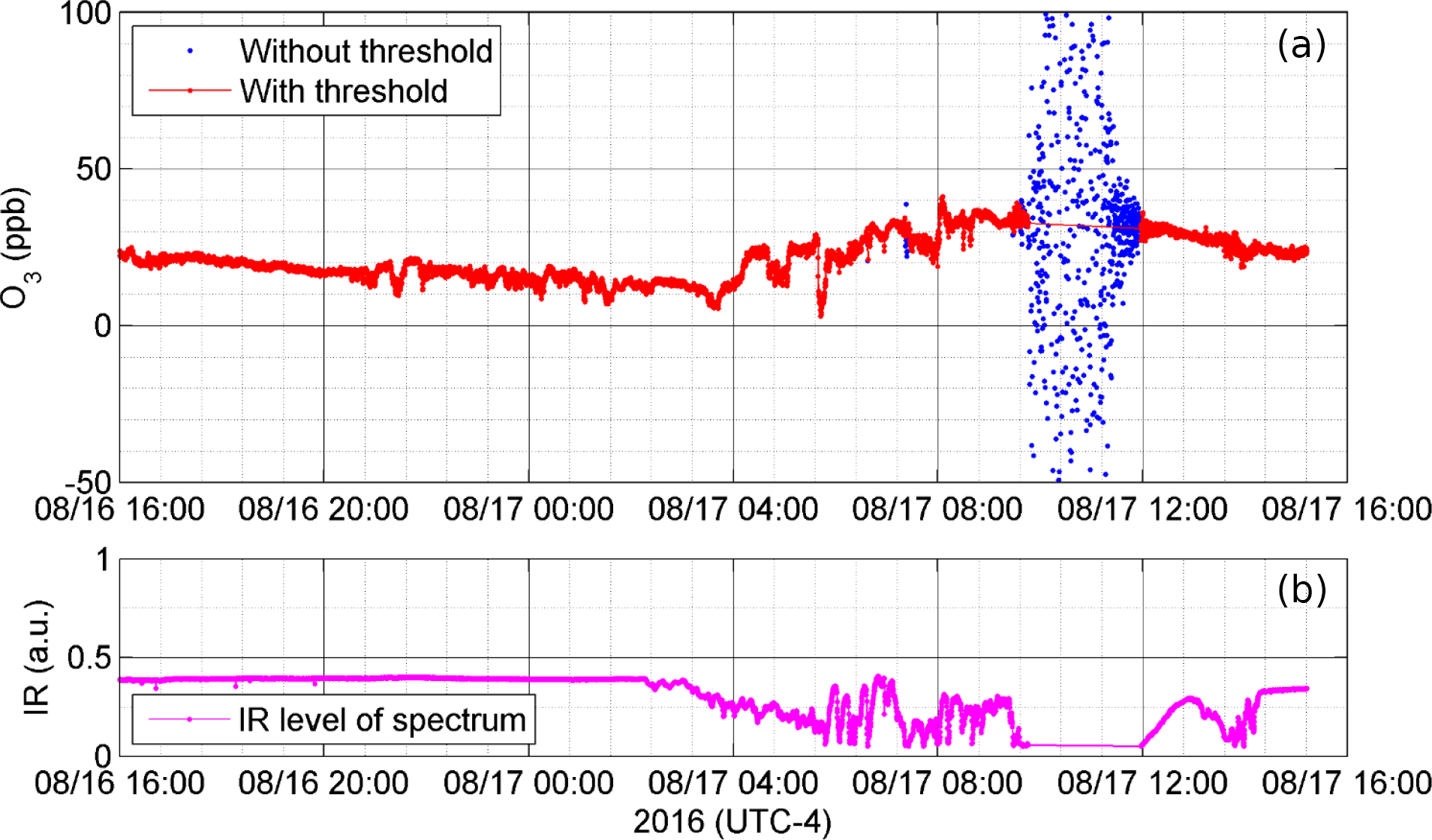
Figure 3Effect of fog and rain on (a) retrieved O3 concentration shown here filtered with and without a minimum spectral signal intensity threshold of 0.05 arbitrary units (a.u.), and (b) the corresponding infrared signal intensity (a.u.) at 2100 cm−1.
2.2 Weather effects in OP-FTIR measurements
While the OP-FTIR measurement tolerates considerable fog and precipitation, as discussed above, when IR signal levels drop to near zero then RMS retrieval residuals increase and retrieved concentrations become very noisy. During August measurements (2016) the system experienced foggy and rainy conditions in the open path, which allowed us to determine a threshold level of IR signal in the spectrum as an objective criterion to screen for heavy fog and rain. When IR signal levels dropped below 0.05 arbitrary units (a.u.) at 2100 cm−1 from a more typical value of 0.4, retrieved O3 concentrations became highly scattered (Fig. 3). However, as long as IR intensities were above 0.05 a.u., retrieved O3 concentrations varied but did not correlate with IR intensity, indicating a true sensitivity of the retrieval to atmospheric O3 variations. (Different OP-FTIR systems will have a different value of the IR intensity threshold, depending on individual system response.) During the period of near-zero IR intensity the wind blew first from the southeast, then south, then southwest, i.e., not directly into the lightly shielded retroreflector (Fig. 2) facing west. Therefore, while we did not have access to the lighthouse to visually inspect the retroreflector at the time, signal levels appear to have been primarily reduced on account of water droplets in the open path as opposed to coating the retroreflector cube corners, which can also happen under strong winds towards the retroreflector.
2.3 NAPS measurements of trace gases
The NAPS program was established in 1969 to monitor and assess the quality of ambient (outdoor) air in populated regions of Canada. The target air pollutants include CO, O3, NO, NO2, SO2 and PM, which are reported hourly but available per minute from NSE upon request. VOCs are measured on a 6-day rotating cycle by 24 h canister sampling and laboratory analysis. There are two NAPS stations in Halifax Regional Municipality: one in downtown Halifax ∼300 m from Halifax Harbour, and another at a suburban background location ∼11 km northeast of Halifax Harbour. (Only the downtown station samples and reports VOCs.) The downtown NAPS station is ∼1 km from the OP-FTIR measurement site (Fig. 1); thus, it measures very similar air masses, but is subject to downtown vehicle traffic and the influence of flow around mixed-height buildings. Due to the shape of the Halifax Peninsula (Fig. 1), ship emissions can most easily reach both the NAPS and OP-FTIR sites by north, northeast, east, and southeast winds, although the NAPS station is ∼300 m (and three roads) inland from the harbour and as such is always sampling a mixture of vehicle and marine emissions. South winds are likely to bring marine emissions to the OP-FTIR instrument from the South End Ship Terminal while bringing more direct downtown vehicle emissions to the NAPS station. Northwest winds are likely to bring a mixture of shipping and vehicle emissions to both OP-FTIR and NAPS measurement locations. Finally, west and southwest winds mostly likely bring vehicle emissions to both the OP-FTIR and NAPS measurement locations.
The NAPS station is located on a relatively small (two-lane) but very busy downtown street that primarily serves as a corridor for light duty vehicles and 14 city bus routes, with a bus stop ∼80 m away to the north and ∼50 m away to the south. Gaseous air pollutants (NO, NO2, CO, O3, SO2) were sampled through an inlet on the fourth floor of a building adjacent to the road, ∼10 m above car exhaust and ∼8 m above bus exhaust plumes. Therefore, both hourly average and particularly per minute measurements of CO, NO, and NO2 concentrations are strongly influenced by instantaneous traffic density. Measured O3 concentrations are also expected to respond (inversely) to traffic density due to the fast titration by NO. However, the inverse response of O3 is expected to be slower and more spread out in time than CO, NO and NO2 given that the lifetime of NO against the O3 titration reaction is ∼76 s at 298 K and 30 ppbv O3 (4–6 min for conversion of >99 % NO to NO2) (McLaren et al., 2012).
Table 2Assumed ship types and engine loads for emissions calculations, following United States Environmental Protection Agency (2000).
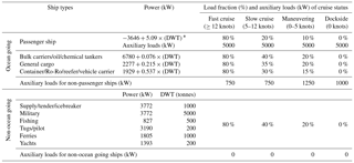
* DWT represents deadweight.
2.4 Emission plume detection
During field measurements, the information on ship positions was collected in real time from AIS signals transmitted by ships, as displayed by http://www.marinetraffic.com, last access: January 2017. The information included ship type, deadweight, name and tracks in and near Halifax Harbour (latitude, longitude, time and speed, updated every 2–3 min when close to a land-based receiver). We used this information to calculate ship emission rates (kg min−1) for all of the gases in Table 3 and correlate them in time with concentration variations measured by OP-FTIR in units of parts-per-million (ppmv) or parts-per-billion (ppbv) by volume, accounting for ship position, wind speed and direction. Specifically, we identified ship emissions as containing enhanced CO2, CO, NO, NO2 and reduced O3, as done by many other authors, e.g., Lu et al. (2006) in the detection of shipping plumes drifting more than 5 km inland in Vancouver.
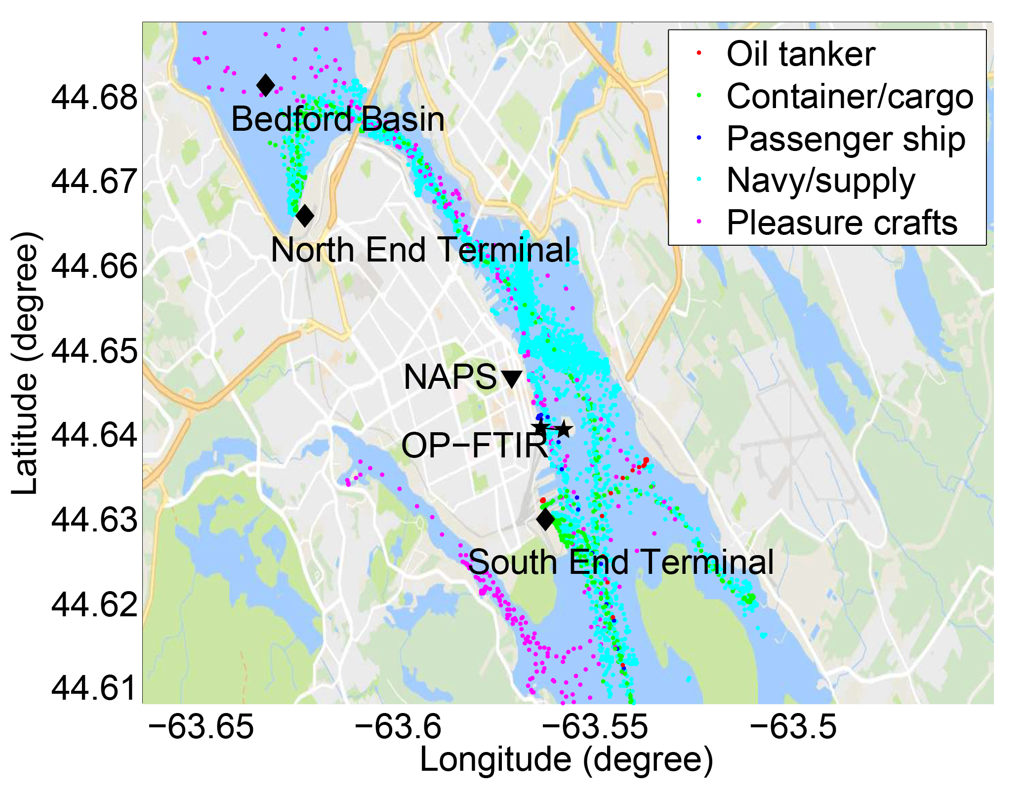
Figure 4Distribution of ship activities during the 15–18 August field measurements, not including ships not equipped with AIS transponders (e.g., small pleasure craft, municipal ferries).
Table 3Emission factors for ship emissions calculations, following United States Environmental Protection Agency (2000). FSC is the fuel sulfur content (% m m−1), set to 0.1 % as per applicable SECA regulations in the calculation region and time.
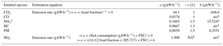
a n/s represents not statistically significant. b NA represents not available. c NOx emission rate gives the NO2-equivalent mass of emitted NOx.
Table 4Ships in Halifax Harbour during field measurements at Halifax Seaport and their calculated emissions.
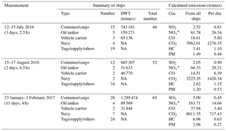
* NOx is expressed as NO2-equivalent mass
2.5 Total emissions calculations
We used AIS information on ship type, cruising status and deadweight to calculate exhaust gas emissions (kg min−1) from different types of ships according to a commonly used parameterization (United States Environmental Protection Agency, 2000) for ship power and load fraction (Table 2) and energy-based emission factors (Table 3). A summary of vessel types in port, including their deadweight and the integrated emissions (tonnes) during the measurement period, is shown in Table 4. CO2 is the highest emitted gas by mass, with CO emissions comprising <0.5 % of CO2 emissions, as expected for high temperature combustion, which also leads to high NOx emissions. Calculated NOx emissions represent both NO and NO2 expressed as NO2 equivalent mass, assuming 100 % conversion of NO to NO2, for better comparison to emission inventories. Finally, SO2 emissions were calculated for an FSC of 0.1 %, the maximum permitted for ships in port during the measurement period. As such, calculated SO2 emissions represent a conservative estimate.
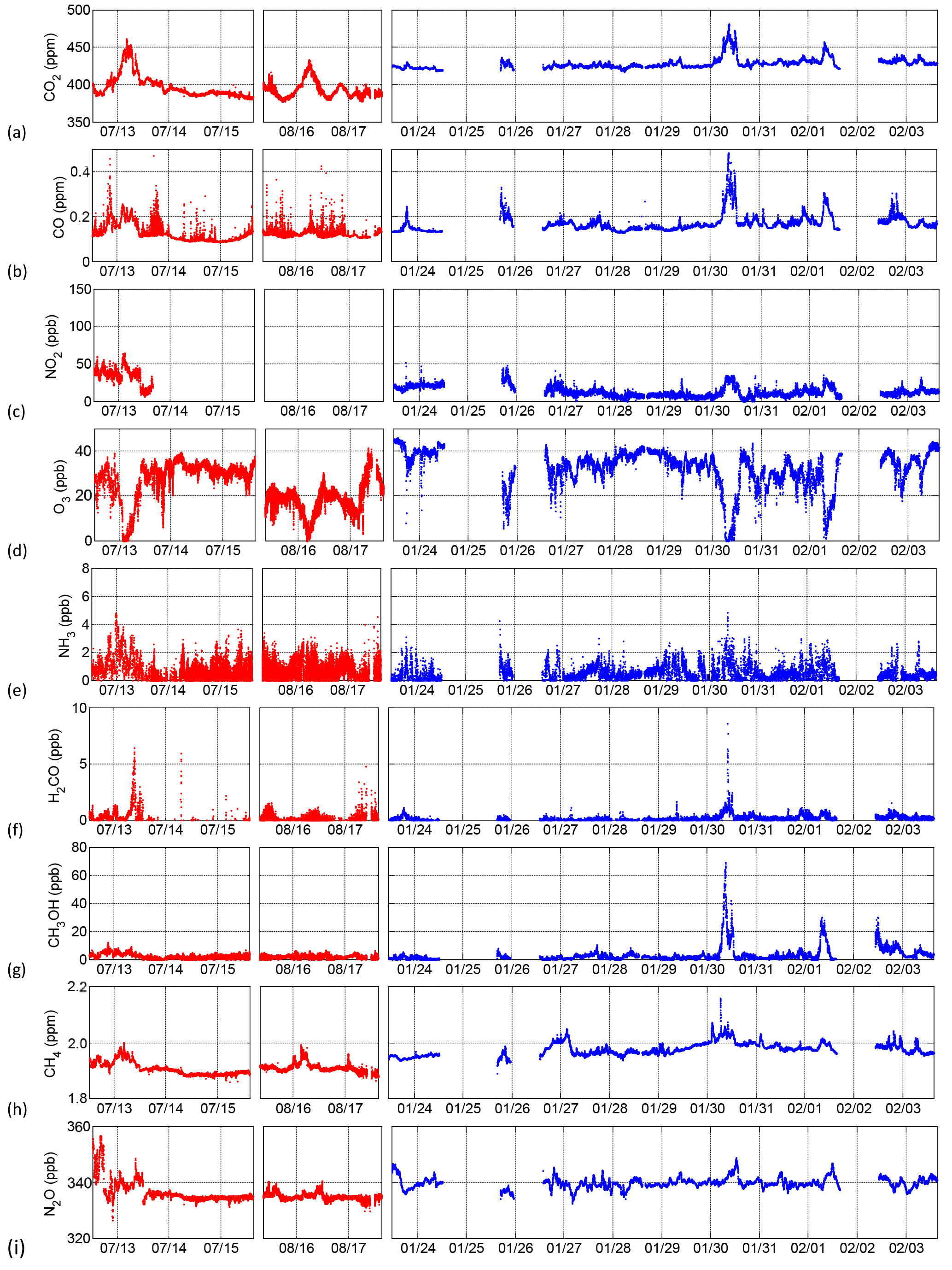
Figure 5Retrieved concentrations of trace gases during summer (red) and winter (blue) field measurements.
3.1 Overall characteristics of the dataset
In 2016, open-path FTIR measurements of trace gases were conducted in summer conditions from 12 to 15 July, and again from 15 to 17 August. Winter observations (lower atmospheric water vapour and less spectral interference, reduced mixing layer height, slower photochemistry, suppressed biogenic emissions) were conducted from 23 January to 3 February 2017. Figure 4 shows the distribution of ship activities during the three measurement periods based on AIS signals, while Table 4 shows a summary of ship types along with calculated total emissions (tonnes). Due to winter storms, the winter measurement was interrupted from 24 to 26 January and from 1 to 2 February 2017. Retrieved concentrations of CO2, CO, NO2, O3, NH3, HCHO, CH3OH, CH4 and N2O are shown in Fig. 5. All time stamps presented in this work are in UTC−4, that is, without DST in summer. The temporal resolution was 1 min in winter and also in summer prior to 16:00 on 13 July, at which point it was increased to 10 s. This caused reduced repeatability (increased scatter) and a bias in retrieved NO2 values after 16:00 on 13 July (not shown), but it did not strongly affect other gas time series (CO2, CO, O3, CH4, N2O) on account of their higher information content (greater target absorption, less water interference) in the underlying spectra. Finally, summer measurements were recorded at ∘C and while winter measurements were recorded at and .
Concentrations of CO2 and all other retrieved gases except O3 show (Fig. 5) various degrees of enhancement on 13 July, 16 August, 30 January and 1 February during broad periods (∼9 h) of low wind speeds and suppressed mixing. O3 is completely or almost completely titrated during these extended time periods. CO shows the same broad enhancements in addition to many relatively narrow enhancements on summer afternoons, related to pleasure craft in the harbour (Sect. 3.5). NH3 concentrations show some enhancement when CO2 is enhanced but are highly variable in both summer and winter, as is HCHO; however, HCHO experiences stronger relative enhancements than NH3, pointing to the proximity of more concentrated sources to the measurement location. CH3OH, like HCHO, shows strong enhancements correlated with times of suppressed mixing but only in winter, with summer background concentrations slightly higher than winter, especially on 12 and 13 July. Finally, CH4 and N2O are elevated when CO2 and CO are elevated, implying similar sources.
We assessed the spectral signatures of several gases other than those reported in Fig. 5. Due to strong interference from absorption by atmospheric water vapour, NO was impossible to retrieve reliably except in winter measurements during times of greatest enhancement (30 January and 2 February). As such, the time series of NO is not shown. Similarly, SO2 is highly susceptible to strong water vapour spectral interference and not possible to retrieve reliably even with our long path length of 910 m – this is due in part to the now very low FSC (0.1 % m m−1) used by ships during our measurement period. Nevertheless, we are continuing to systematically study the sensitivity of the OP-FTIR SO2 retrieval to water interference and other retrieval parameters and intend to expand on this in a future publication outlining when and where the retrieval may be successful using the technique. We also retrieved HNO3, HONO, C2H6, C2H4 and C2H2 with mixed success. HNO3 (1235–1340 cm−1) was subject to similar water interference issues as SO2. HONO (1220–1300 cm−1) was below detection limits at all times, even during the extended emissions accumulation periods on 30 January, when water vapour interference was at a minimum. C2H6 (2900–3005 cm−1), C2H4 (940–960 cm−1) and C2H2 (725–775 cm−1) showed some accumulation during periods of low wind speed; however, the retrievals require further work and independent measurement verification, beyond the scope of this study.
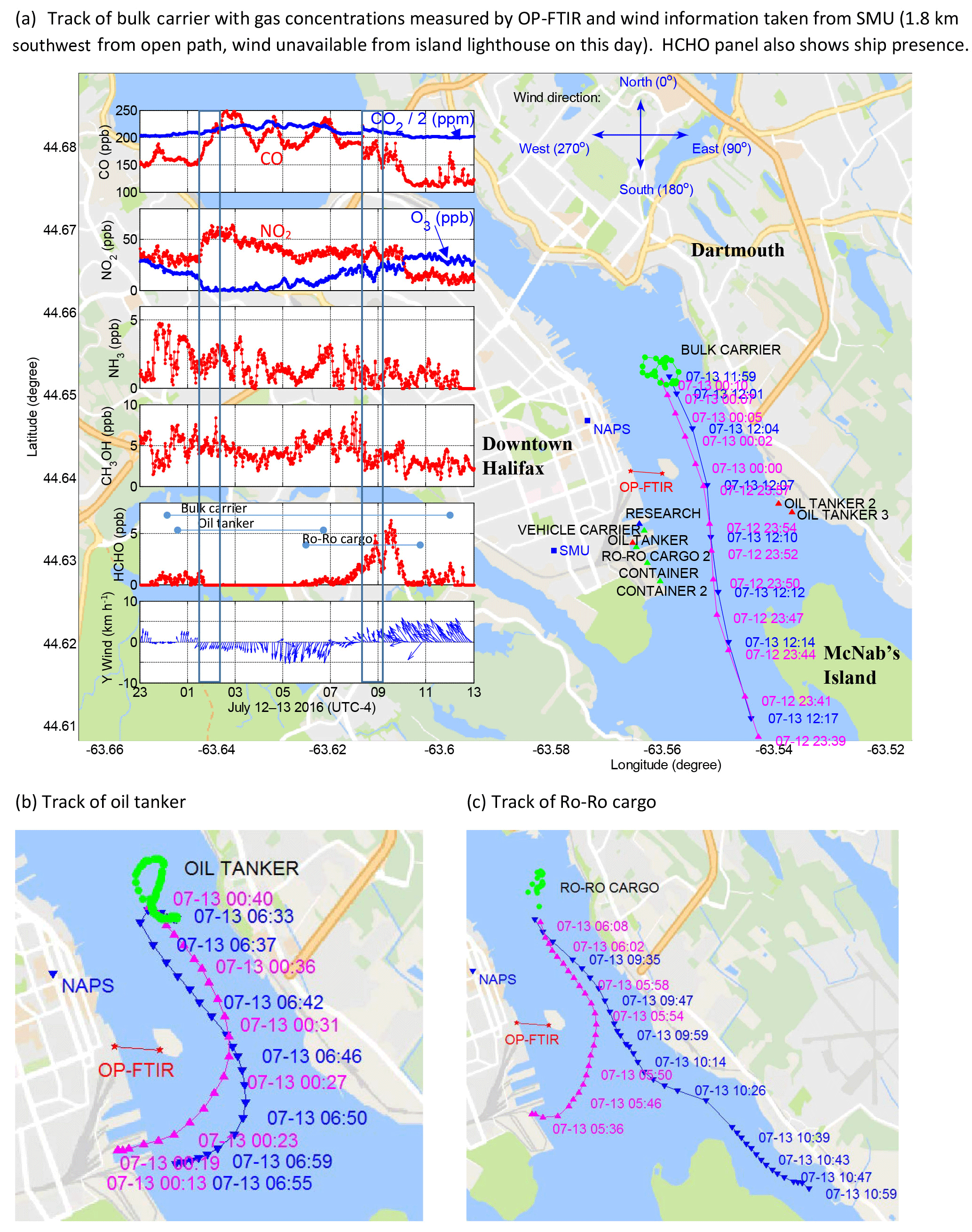
Figure 6Measured trace gas concentrations and main ship activities during extended emissions accumulation of 13 July 2016. Ship arrival (pink triangles), departure (blue triangles) and maneuvering (green dots) shown for main ships only. (a) Track of bulk carrier with gas concentrations measured by OP-FTIR and wind information taken from SMU (1.8 km southwest from open path, wind unavailable from island lighthouse on this day). HCHO panel also shows ship presence. (b) Track of oil tanker. (c) Track of Ro-Ro cargo. Y wind represents the north–south wind magnitude.
3.2 Accumulation of emissions in summer
A strong enhancement of CO2 was recorded from 00:00 through to noon on 13 July, associated with light winds and an enhancement of CO, NO2, CH4 and N2O, as well as a complete titration of O3 lasting ∼6 h (Figs. 5d, 6a). CH3OH and NH3 concentrations were enhanced in and around the time interval from 00:00 to 12:00 but do not correlate as strongly with the CO2 enhancement as the other gases. HCHO was enhanced but only near the end of the broad CO2 enhancement. Although Halifax is surrounded by forests (Fig. 1) and July is in the peak of the growing season, the enhancement of CO2 beginning after midnight and associated with O3 titration is inconsistent temporally and chemically with plant respiration of CO2, which would be expected to occur earlier (i.e., from 18:00 onwards as is the case in unpublished data acquired with our system in a forest environment only 12 km away) and not affect O3 concentrations. Winds were light and from the north to northeast, which is the direction of built environments extending for ∼10 km. The timing of the event is also not consistent with morning traffic emissions (on a Wednesday), which would be expected to start accumulating after ∼06:00, not earlier during the night.
From ∼00:00 to ∼12:00 on 13 July a bulk carrier ship maneuvered north of George's Island at a distance of ∼1.5 km to our measurement open path (Fig. 6a). From ∼00:15 to 07:00 a harbour service oil tanker navigated to the same area and refuelled the bulk carrier (Fig. 6b). At ∼06:00 a Ro-Ro cargo ship voyaged to 1.8 km north of the measurement open path (300 m north of the bulk carrier and oil tanker) and undertook a short-term cruise in that area until ∼09:30 (Fig. 6c). The tracks of these three ships were all arriving from the south or southeast towards the area north of George's Island and departing in the opposite direction (Fig. 6).
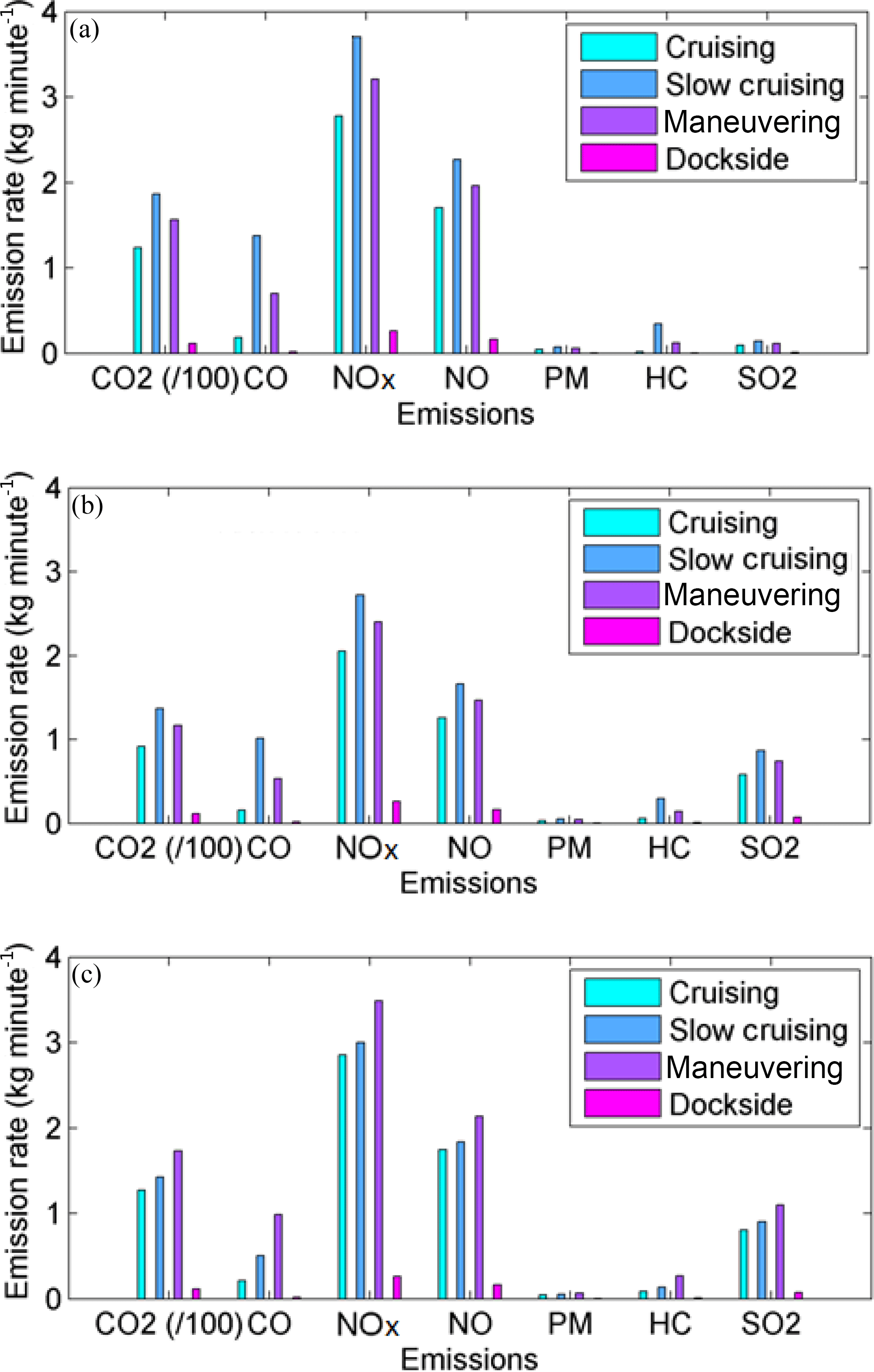
Figure 7Calculated range of emissions for different operating modes of (a) bulk carrier, (b) oil tanker and (c) Ro-Ro cargo using the emissions model from Tables 1 and 2. NOx represents NO2-equivalent mass.
We calculated the theoretical emissions of trace gases (kg min−1) from each of the three ships in all operation modes (dockside, maneuvering, slow cruising and cruising) north of George's Island in terms of CO2, CO, NOx, NO, SO2, HC and PM (Fig. 7). While the ships vary considerably in gross tonnage and deadweight, they have comparable emission rates. As shown in Fig. 6a, while the bulk carrier and oil tanker were north of George's Island and the wind was from the south there was no significant trace gas enhancement. Only when the light wind changed to northeast at 01:20 did the concentrations of CO and NO2 increase, while O3 decreased to 0 ppbv due to titration by NO () in freshly emitted combustion plumes (e.g., Brown and Stutz, 2012). The concentrations of CO fluctuated in rough agreement with the wind direction and the location of sources until 04:00 while NO2 variations were smoother, possibly because of other chemical processes, e.g., once O3 is completely titrated no further conversion of NO to NO2 is possible, but night-time conversion to NO3, N2O5 and HNO3 (McLaren et al., 2010) as well as heterogeneous conversion to HONO and HNO3 may be taking place (Wojtal et al., 2011). We note that on 13 July twilight occurred at 04:06 (UTC−4; 05:06 ADT) and sunrise at 04:41 (UTC−4; 05:51 ADT) at which time photolysis of NO2 () increased in importance (e.g., Jacob, 1999) and O3 began increasing even though CO also increased from 04:00 to 05:00, as did the wind speeds. A pilot and military patrol vessel passed under the open path at 04:15 and 04:19, respectively, with only slight variations in CO. The increase of CO from 06:00 to 07:00, when the wind was north/northeast was likely caused by (1) the Ro-Ro cargo arriving at 06:00, (2) the oil tanker leaving at 06:35 and (3) traffic emissions increasing across the Harbour in Dartmouth. By 07:30 the winds were very light again and the baseline concentration of CO was ∼200 ppbv as compared to ∼150 ppbv at 01:00, likely reflecting accumulating morning traffic emissions in both downtown Halifax and Dartmouth.
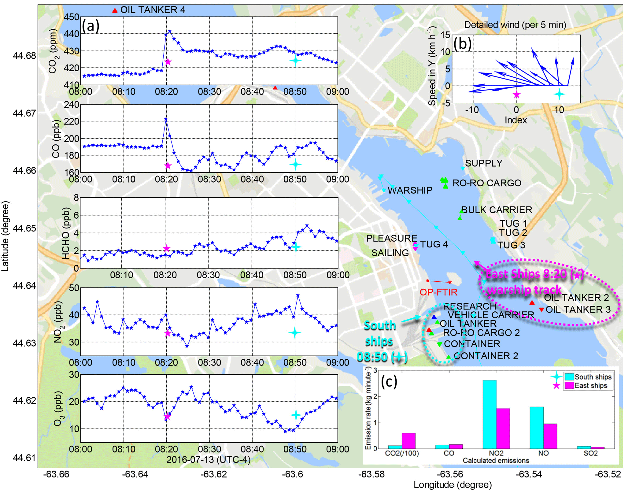
Figure 8Detailed analysis of trace gas concentrations on 13 July (a) under slowly changing winds (b) from 08:00 (time index 0) to 09:00 (time index 10) as emissions from two clusters of ships (c) were calculated based on their instantaneous AIS activity report at 08:20 (“East ships”: warship = slow cruising; oil tanker 2 & 3 = dockside) and 08:50 (“South Ships”: dockside).
After 08:00 wind speed increased and wind direction changed slowly from north/northeast to east/southeast and finally south (Fig. 8b, from time index 0 to 10). A pilot vessel passed under the open path at 08:09, but there was almost no effect on CO2 and CO concentrations at that time (Fig. 8a). Trace gases over the measurement open path were no longer impacted by emissions from the bulk carrier and Ro-Ro cargo (north of the open path) nor by Halifax/Dartmouth vehicle traffic emissions, but instead first (08:20) by one slow cruising navy warship (Fig. 8a) at ∼0.7 km on nearest approach and two additional moored oil tankers at ∼2.1 km to the east/southeast (Fig. 8a), and then (08:50) by six ships moored ∼0.7–1.5 km to the south (Fig. 8a), including the oil tanker that had refilled the bulk carrier earlier, which was now dockside. Winds from the south would also bring emissions from heavy duty diesel engines of trucks operating at the container terminal in the south, and other loading and port vehicles and machinery. We estimated the combined instantaneous emissions of CO2, CO, NOx, NO and SO2 of the navy warship together with the two additional oil tankers based on available AIS status information and added them together as “East ships” in Fig. 8c. Some AIS information on navy vessels is classified, so we assumed a deadweight of 5000 t and designated its emission model as that of an offshore supply ship (Table 2). Similarly we estimated the combined instantaneous emissions of the six docked “South ships” (Fig. 8c). The CO emissions of the “East ships” and “South ships” are comparable; however, measured CO perturbations at 08:20 with an east wind (Fig. 8a), when the navy ship slowly cruised east of the measurement path with two additional oil tankers ∼1.4 km further east, were larger and sharper than CO perturbations measured at 08:50 with a south wind and six docked “South ships”. It appears that the least diluted emissions of the navy warship also dominate the trace gas response at 08:20 in terms of elevated CO2, slightly elevated NO2 and slightly decreased O3. Conversely, trace gases detected in the open path at 08:50 show a more dilute response in CO2 and CO but a more pronounced increase in NO2 and decrease in O3, consistent with the 1–5 min transport time of “South ship” emissions to the measurement open path. We do not have information on any exhaust after treatment used by the vessels analyzed, although this would not affect CO2 levels, only NOx, CO, HC, SO2 and particle levels (Pirjola et al., 2014, and references therein).
While our measurements of ship emissions showed that HCHO was below detection limits from 02:00 to 06:00 when the bulk carrier and the oil tanker were maneuvering under winds favourable for detection in the open path, it has previously been noted (Agrawal et al., 2008b; Reda et al., 2014) that HCHO is the dominant emitted aldehyde from ship engines burning both heavy fuel oil and distillates, and it has also been detected in the field (Williams et al., 2009). The late morning HCHO enhancement (08:00–10:00) is also associated with an enhancement of CO and NO2 and a decrease of O3 (Fig. 6a, grey box) from approximately 08:15 to 09:15 (peak HCHO ∼5 ppbv), while winds remain relatively light and from the south or southeast (Fig. 8b). At 09:15 HCHO, CO and NO2 are markedly reduced while O3 increases (as winds increase), after which HCHO peaks again (∼6 ppbv HCHO) at 09:30 together with CO and NO2 while O3 is slightly reduced. The HCHO is presumably of anthropogenic origin, with the majority likely from secondary production (Luecken et al., 2012) via oxidation of accumulated precursors (CH4, other alkanes, alkenes and VOCs). Our CH3OH measurements show increased values at 08:00 (Fig. 6a) but no correlation to HCHO, and both gases are markedly reduced at 10:00 as wind speeds increase, bringing background marine air to the measurement path with background O3 concentrations. Williams et al. (2009) postulated that a buildup of HCHO during the night may be important in leading to an increased source of HOx radicals in the morning; however, we do not find evidence of extensive HCHO accumulation during the bulk of the 13 July CO2 enhancement (from 02:00 to 07:00, Fig. 6a) under direct ship influence of the measurement path and low wind speeds, but instead only from 08:00 to 10:00.
As briefly noted earlier, throughout the broad night-time period of enhanced CO2 concentrations (00:00–12:00) both NH3 and CH3OH levels (detailed view in Fig. 6a) were also enhanced but not clearly correlated with CO, except possibly for NH3 from ∼01:20 to 02:20 (likely due to ship emission advection) and again from 06:00 to 07:00 (likely due to mounting vehicle traffic). It is difficult to definitively attribute NH3 enhancements to either ships or vehicles in the study area. In an older study, Burgard et al. (2006) found NH3 emissions of 0 g kg−1 (within error) in the exhaust gas of diesel engines operating on roads (∼0.5 g kg−1 for gasoline engines); however, NOx reduction technologies for diesel engines are evolving, as are the exhaust emissions (Piumetti et al., 2015). While Suarez-Bertoa et al. (2014) measured NH3 emission factors from a single diesel car engine (equipped with SCR NOx control, a diesel oxidation catalyst and a diesel particle filter) that were higher than some gasoline car engines, Carslaw and Rhys-Tyler (2013) show in a study involving 70 000 vehicles that NH3 emissions are most important for catalyst equipped gasoline vehicles and SCR-equipped buses, with gasoline engine NH3 emissions ∼6 times higher than diesel engine NH3 emissions for newer car models (>2010). Conversely, SCR in ships operating with heavy fuel oil may also be a source of ammonia in the exhaust due to ammonia slip, which is currently not regulated in ship applications by the IMO (Lehtoranta et al., 2015).
Finally, CH3OH has strong biogenic sources related to plant growth and decaying plant matter, as well as from the marine biosphere, which is a large gross source but an overall net CH3OH sink (Hu et al., 2011). It is also formed from CH4 oxidation, which is also a globally important source of CO and HCHO, although this reaction is relatively slow and mainly proceeds in low NOx environments (de Gouw et al., 2005). CH3OH has strong primary and weak secondary urban sources (de Gouw et al., 2005) and the main sink is by OH oxidation (Hu et al., 2011). Rantala et al. (2016) show CH3OH concentrations correlated with traffic emissions in all seasons and of 100 % anthropogenic origin during the winter and 42±8 % during summer, when biogenic influences play a large role. Our measured CH3OH concentration shows the same nearly monotonic rise from 06:00 to 07:00 as NH3 and CO (Fig. 6a), as light winds from the north and northwest brought traffic emissions to the measurement path. Throughout the 13 July enhancement of CO2, CH3OH was elevated but highly variable, showing only occasional correlations with narrow CO spikes (Fig. 6a) and its enhancement extends both before 00:00 and after 12:00 on 13 July (Fig. 5g). This suggests a blending of biogenic, vehicle traffic and shipping emission sources in the summer data.
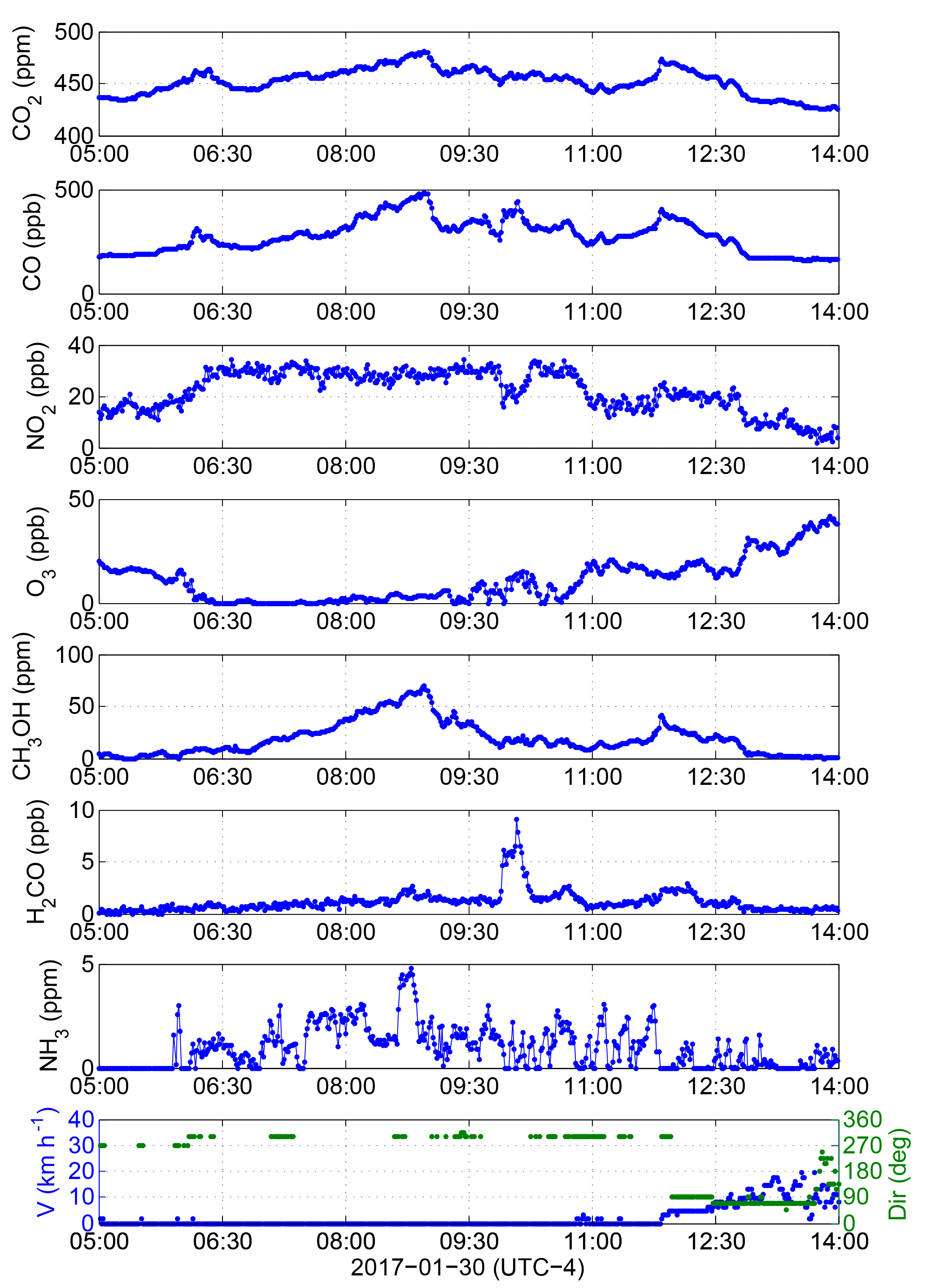
Figure 9Measured trace gas concentrations during extended emissions accumulation on 30 January 2017. Wind direction (bottom-most panel) before 12:00 is missing or highly variable because the wind speed is ∼0 km h−1.
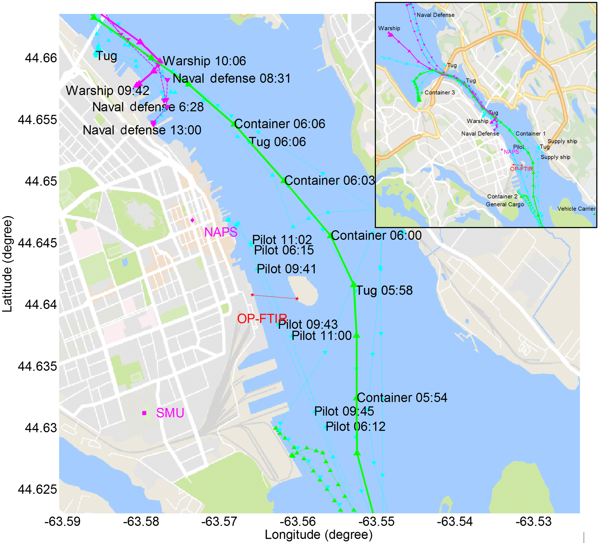
Figure 10Major ship activities during extended emissions accumulation on 30 January 2017, with only selected time stamps shown for increased clarity to the immediate right of a given ship track coordinate marker. Container or cargo shown in thin or bold green, navy ships in solid or dashed pink, tugs or supply vessels in solid cyan and pilots in dashed cyan.
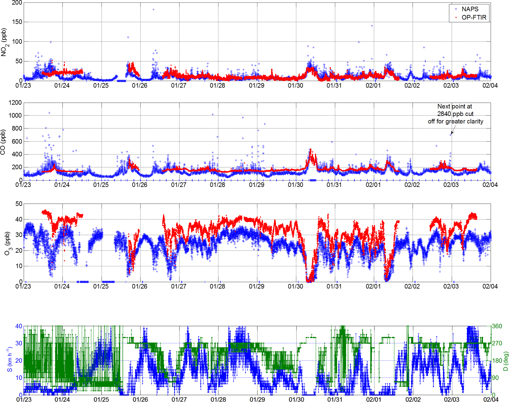
Figure 11Comparison between trace gas concentrations measured in Halifax from 23 January to 3 February 2017 at the NAPS station (in situ measurement, ∼300 m from harbour, strongly influenced by vehicle traffic) and with OP-FTIR system ∼1 km away (455 m open path measurement, spanning across harbour water, less influenced). Zero values in the NAPS measurements represent periods of calibration or no data (e.g., on 30 January for CO). Bottom panel shows wind speed and direction during the time period, measured at retroreflector with OP-FTIR system.
3.3 Accumulation of emissions in winter
A strong enhancement of CO2 was also recorded on 30 January from 05:00 to 14:00 (Fig. 5) on a windless morning (Fig. 9) with busy harbour activities of 23 vessels (Fig. 10 and inset). Ship and other emissions were accumulated in the surrounding area and were measured by the OP-FTIR system (Fig. 9) as well as the NAPS monitoring station ∼1 km away (Fig. 11, Sect. 3.4). There were no ships maneuvering or moored immediately north of George's Island on 30 January (unlike the 13 July); instead, vessels cruised in the shipping channel (Fig. 10), including through the measurement open path. From 05:00 to 09:00 concentrations of CO2 and CO rose almost monotonically as Monday rush hour mounted, with a perturbation between 06:00 and 06:30 from container ship 1 as it navigated to the North End Terminal (5.9 km to OP-FTIR) passing outside of George's Island at 06:00. During this half hour period NO2 increased and remained elevated until 10:00 while O3 reduced to 0 ppbv and remained titrated until 09:30. Sunrise occurred at 07:35 (twilight at 07:03). The variable but increasing NH3 concentration from 06:00 to 09:00 indicates that these air pollutants might be from the accumulation of emissions from vehicle traffic due to the mounting rush hour. There is also a very distinct accumulation of CH3OH during this time, which has known correlations with vehicle traffic and may be related to gasoline methanol content (Rantala et al., 2016) and to windshield wiper fluid which is used more frequently in winter months (Carrière et al., 2000), while accumulation is less apparent for HCHO.
From the time series profile of CO at the time of container ship 1 passing by our measurement location (heading north-northwest) we infer that a weak breeze from the northwest must in fact have been present, even though the wind sensor was registering 0 km h−1, with very occasional readings of 1.6 and 3.2 km h−1 (Fig. 9). This made it possible for the open path to sample emissions from the northwest, which was the heading of container ship 1, which changed status to maneuvering at 06:34, moored at 06:54 and became dockside at 07:19. At this point in time the vessel was located in the North End Terminal, ∼6 km away, and separated from the open path by a portion of the land mass of Halifax Peninsula (Fig. 1), which would make the attribution of concentration changes solely to shipping emissions implausible. However, emissions from ships can rise 2–10 times the stack height and experience vertical mixing on timescales of 20–40 min, possibly filling the entire boundary layer height, depending on buoyancy flux and boundary layer stability (Chosson et al., 2008). As such, it is not impossible to have detected some shipping emissions from several kilometres away on a still January morning.
A pilot ship also crossed the measurement path at 06:15, and again at 09:41 and 11:01 (Fig. 10) but did not produce significant signatures in trace gas concentrations. Also in the early morning a navy coastal defense vessel (55.3 m length) changed status from mooring to maneuvering at 06:28 at its berth location 2.1 km northwest of the OP-FTIR (Fig. 10). It left the berth in slow cruising mode at 08:31 until 09:03 when it reached the Bedford Basin 8.6 km northwest of the OP-FTIR. Based on the very low wind speed, it would take 1–2 h for its departure emissions to advect to the measurement open path. The navy defense vessel returned from the Bedford Basin at 11:33 in slow cruising mode, arriving at berth at 12:15 in a slightly closer (1.9 km from the OP-FTIR) location and turning its engines off at 13:00.
From 09:50 to 10:10 concentrations of HCHO were significantly elevated, with a modest increase in CO, a decrease in NO2 and an increase in O3 during the same time. A navy warship (134.2 m length) started maneuvering near its berth (2.3 km from the OP-FTIR) from 09:41 to 10:03 and then left the berth (Fig. 10) in slow cruising mode at 10:10 heading for the Bedford Basin (8.9 km from the OP-FTIR). Under the light winds it would take ∼1 h for emissions from the warship to reach the measurement open path, experiencing dilution along the way; therefore, it is unlikely that the sharp rise in HCHO at 09:50 (Fig. 9) is due to the warship. As already mentioned, a pilot ship also crossed the measurement path at 09:41 heading southeast; however, the same pilot ship had crossed the open path at 06:15 and 11:01 (Fig. 10) at a similar speed and there had been no enhancement in HCHO registered at these times (Fig. 9). As such, the origin of the strong HCHO enhancement is ambiguous and requires further field study. An event of increased CO2, CO, NO2 and CH3OH at 11:50, with a broader increase in HCHO over the next 20 min is also not clearly related to ship activities, motivating further field study.
From 11:00 onwards increasing wind speeds and mixing dissipated accumulated pollutants, while the wind direction changed to easterly winds after 12:00 (Fig. 9). At 07:00 container ship 2 voyaged from the mouth of the harbour to the South End Terminal (1.2 km to OP-FTIR); however, the emissions of this vessel are unlikely to impact the measurement path due to the weak northwest breeze. The same can be assumed for the emissions of a general cargo ship at 11:00 (3 km from the OP-FTIR).
3.4 Comparison to NAPS in situ data in downtown Halifax
Our OP-FTIR measurements were conducted ∼1 km from the downtown Halifax NAPS station influenced by vehicle traffic, as described in Sect. 2.3 and Fig. 1. The NAPS site is influenced by vehicle traffic emissions during all wind conditions, including those most directly from the harbour (north, northeast, east, southeast, south), which lies ∼300 m to the east and three busy streets away from the NAPS station. In contrast, the OP-FTIR system is most directly influenced by ship emissions, except under winds from the downtown core (northwest, west, southwest). The OP-FTIR measures trace gas concentrations in a 455 m path average (in this particular measurement campaign);thus, it is less sensitive to instantaneous emissions, which are unlikely to fill the entire open path. Figure 11 shows a comparison between in situ NAPS and OP-FTIR NO2, CO and O3 concentrations from 23 January to 3 February 2017. Similar variations in trace gases are apparent, e.g., the long-duration NO2 and CO enhancements with a simultaneous depletion in O3 on 30 January and 1 February. This points to the extended spatial scale of this effect, which has been described as very local or near-field in land-based studies using in situ detection methods (Merico et al., 2016; Diesch et al., 2013; Eckhardt et al., 2013).
However, there are some notable differences between open path and in situ measurements. First, NAPS in situ measurements show multiple NO2 values in excess of 50 ppbv, whereas the OP-FTIR system measurements do not. This is likely due to a combination of (1) strong vehicle emissions present at the NAPS site but not at the OP-FTIR site, (2) path-averaging of direct emissions by the OP-FTIR system, (3) chemical transformation of NO2 and (4) advection and dispersion of emissions between the measurement sites. Second, NAPS in situ measurements also show strong enhancements in CO values in excess of 500 ppbv, whereas the OP-FTIR measurements do not; however, the baseline of OP-FTIR CO measurements is higher than NAPS by 50–100 %, with the greatest differences during early morning periods before rush hour starts. This large bias is outside of the range of errors of either technique, estimated conservatively at ∼10 % for OP-FTIR and 15 % for NAPS in situ measurements as per the minimum NAPS data quality objectives for CO (Canadian Council of Ministers of the Environment, 2011); however, the particular sensor accuracy at the NAPS site in question is <2 %. If we take CO as a marker of fresh combustion emissions then persistently elevated CO at the OP-FTIR site should correspond to persistently lower O3 concentrations but in fact the reverse is observed (Fig. 11), with OP-FTIR O3 typically 35 % higher than NAPS, except during periods of complete O3 titration on 30 January and 1 February. It is not clear what combination of emission differences, in situ vs. path-average sampling differences, chemical transformation and advection and/or dispersion is causing the persistent CO and O3 biases, which are also evident in summer measurements (not shown). While beyond the scope of this paper, the representativeness of in situ vs. path-average surface measurements is under further investigation and has also been documented by You et al. (2017).

Figure 12Combined effects of small and large ships in field measurements of CO, NO2 and O3 on 13 July 2016 under a stable (southeast) sea breeze (20 km h−1) winds. ESE represents east-southeast, SSE represents south-southeast and SE represents southeast.
3.5 Emissions from small craft compared to large ships
In the summer time series of CO concentrations, especially in late afternoons and early evenings, there are many relatively narrow CO spikes (∼1–15 min, >250 ppb, Fig. 5b) that do not match AIS-based ship activity. We noted pleasure craft in the harbour during the campaign and were able to obtain per minute screenshots from a publicly viewable webcam installed on the roof of a nearby tall building (http://www.novascotiawebcams.com/en/webcams/pier-21/, last access: January 2017), which included the measurement open path. The images confirmed that many CO enhancements were caused by high-speed pleasure craft when they passed under the open path – despite the path-average nature of the OP-FTIR measurement and the short (10 s) acquisition time on the afternoons of 13, 14 July and 15, 16 August. Yet this is consistent with higher CO and lower NOx emissions of gasoline engines (predominant in small craft) as opposed to diesel engines (Henry, 2013). On 13 July the sea breeze was steady, approximately from the southeast and relatively constant at ∼20 km h−1. Figure 12 shows the effects of small craft and large ships in measured concentrations of CO, NO2, and O3 as well as in images from the public webcam. With southeast 20 km h−1 winds trace gas emissions from the 1 to 3 km visible area to the southeast of George's Island would take ∼3–9 min to be transported towards the open path. As such, we found that three out of four significant NO2 enhancements and correlated O3 depletions lasting ∼15 min were associated with large ships 1–3 km to the southeast, except at 19:51 (Fig. 12). Speed boats crossing the open path had the most effect on CO and the least effect on NO2 and O3, as expected, given that there was no time for NO titration of O3 to proceed. One small speed boat had a very pronounced effect on CO (Fig. 12, 17:06) that lasted ∼1.5 min and was consistent with the minimum time to traverse the measurement path at 20 km h−1 (1.4 min). In winter, there were no high-speed pleasure craft in Halifax Harbour and there are correspondingly fewer relatively narrow CO spikes despite the longer time series (Fig. 5b). Our detection of a variety of CO enhancement signatures is in contrast to Diesch et al. (2013) who report none using an in situ technique with an 80 ppb detection limit during a study on ship traffic on the Elbe River in northern Germany.
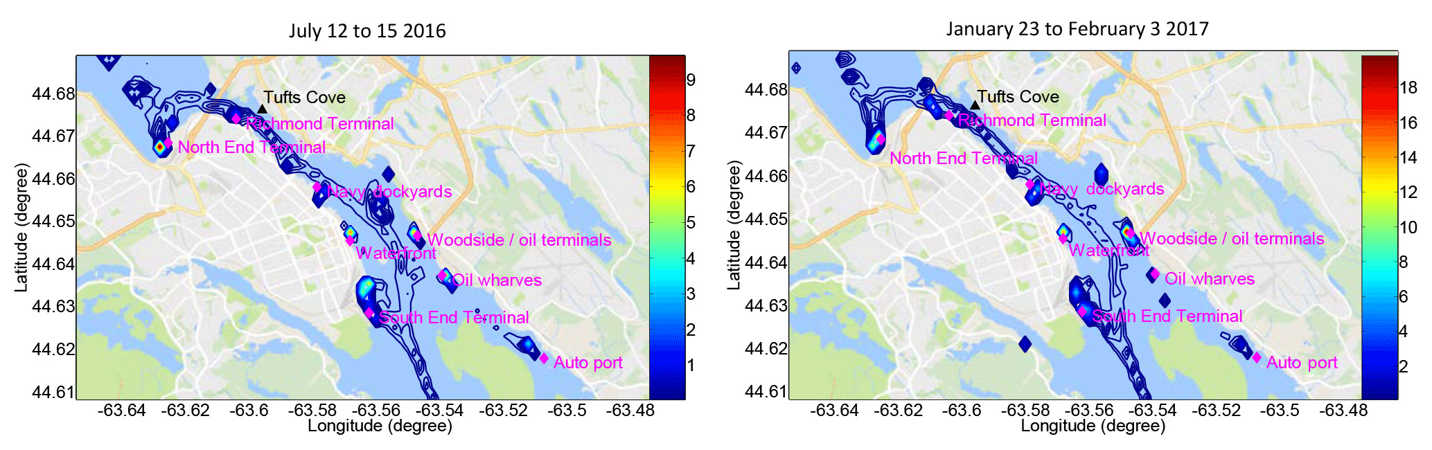
Figure 13Calculated ship emissions (tonnes of NOx expressed as NO2-equivalent mass, shown using unfilled but coloured contours) in Halifax Harbour based on AIS ship type and activity information during variable length summer (July only) and winter (January) measurement periods.
3.6 Distribution of emissions in space, time and by ship type
We calculated ship emissions in Halifax Harbour during the OP-FTIR measurement periods (Table 4) using the emission model from Tables 2 and 3. Figure 13 shows the spatial distribution of NOx emitted during July and January measurements, with emissions clustering predictably around the North End, Richmond and South End terminals, the navy dockyards, the waterfront wharves, the harbour anchorage areas, and two oil terminals and an auto port on the Dartmouth side of the harbour. Emissions of NOx from the South End Terminal are relatively lower in winter due to a lack of cruise ship activity, while emissions from one of the two oil terminals in Dartmouth are relatively higher in winter, likely because heating with fuel oil is common in the city. (Tanker emissions account for ∼15 % of SO2 and NOx emissions in “summer” and ∼19 % of SO2 and NOx emissions in “winter”, as shown in Table 5 and further discussed below). SO2 emissions follow a very similar pattern to NOx emissions and are not shown. As noted, municipal passenger ferry and pleasure craft emissions are not included in the AIS data used in our study; therefore, where emissions appear near ferry terminals they are caused by other vessels such as tugs and coastal supply ships that use the same terminals.
Table 5Calculated marine sector emissions (tonnes) in Halifax Harbour in the “summer” cruise ship season (May 2015–October 2015) and the “winter” off season (non-cruise ship season) (November 2015–April 2016), based on detailed AIS ship type and activity data and the emission model from Tables 2 and 3. Also shown are the percent increases in emitted mass from “winter” (W) to “summer” (S), and the percentage of emissions due to passenger (primarily cruise ship) vessels.
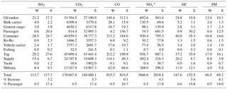
* NOx is expressed as NO2-equivalent mass.
To more fully account for ship emissions by season and type we calculated emissions for a full year using AIS activity data from May 2015 to April 2016, divided into a broad “summer” season when cruise ships are active (May 2015–October 2015) and a broad “winter” season when they are not (November 2015–April 2016). The distribution of NOx and SO2 emissions (Fig. S1 in the Supplement) is very similar to the short measurement time periods shown in Fig. 13 and very similar in “summer” and “winter”, reflecting the location of wharves, terminals and anchorages, with visibly increased emissions from Halifax Seaport in “summer”, where cruise ships are at berth. Table 5 shows the calculated percent increase in trace gas and PM emissions (according to the emission model in Tables 2 and 3) between “winter” and “summer”, with NOx increasing by 4.1 % and SO2 by 3.2 %, as well as the breakdown of this information by ship type. Table 5 also indicates the percentage of these emissions that stem from passenger (i.e., cruise) ships in each season, which is 18 % on average for all species in “summer” and 0.5 % in “winter”. Cruise ship emissions are caused by their high auxiliary loads while at berth (Table 2). Somewhat surprisingly, the greatest proportion of SO2 emissions in “winter” (Table 5) comes from tugs (26 %), followed by container ships (25 %), tankers (19 %) and supply vessels (14 %), while in “summer” this changes to tugs (24 %), container ships (21 %), passenger vessels (17 %) and tankers (15 %). The proportions are very similar for NOx as well as for CO2, CO, HC and PM in “summer” and “winter” (Fig. 14, Table 5). In total, the combined contribution of tugs and coastal supply ships to total SO2 and NOx emissions in Halifax Harbour was ∼40 % in “winter” and ∼30 % in “summer”. In our calculations all coastal (non-ocean going) ships have zero emissions at berth (speed = 0, auxiliary load = 0, Table 2); therefore, their high emissions are related to frequent arrivals, departures and maneuvering.
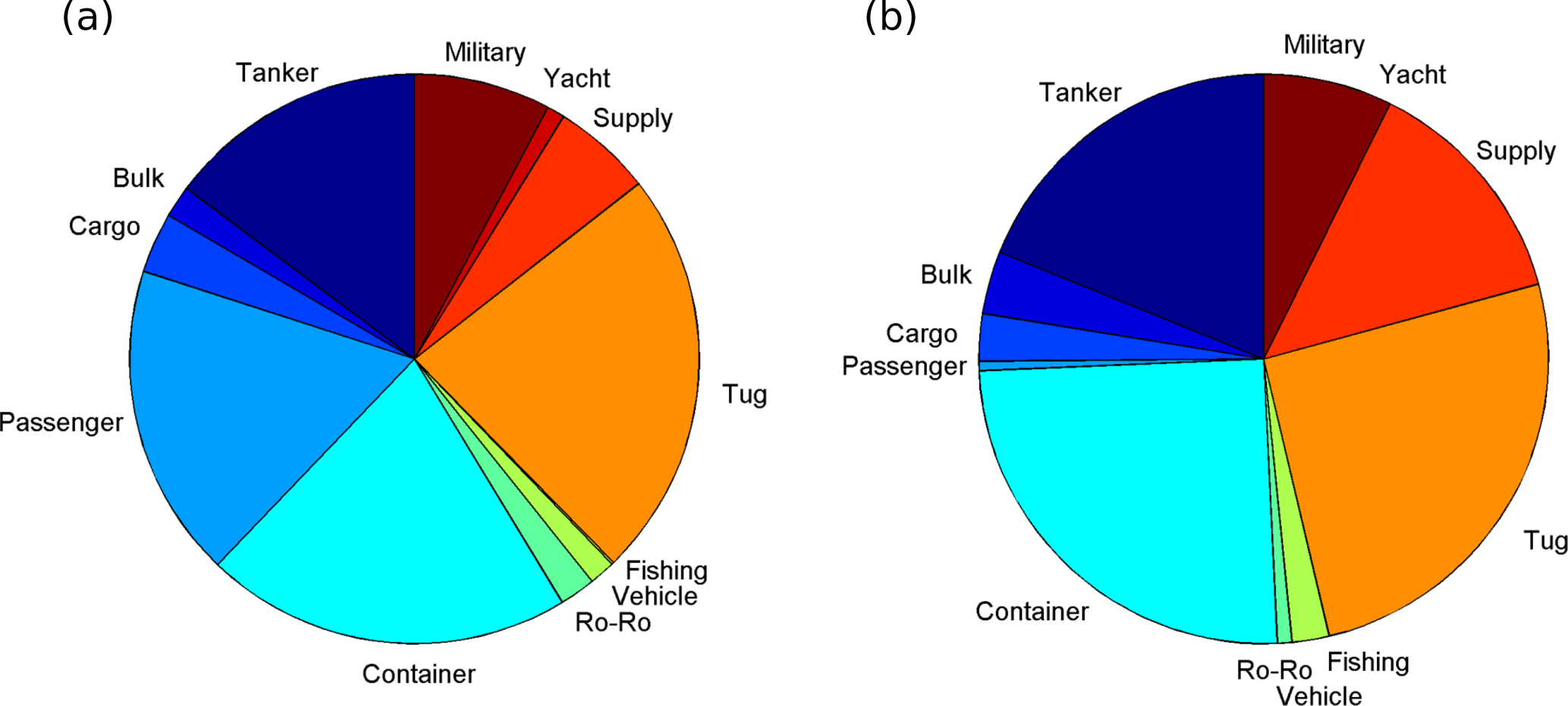
Figure 14Proportion of NOx emissions from different ship types in “summer” (May 2015–October 2015, a) and “winter” (November 2015–April 2016, b).
3.7 Comparison of shipping emissions to other sources
Finally, we compare our calculated emissions to the largest stationary source emitter in the Halifax/Dartmouth area, which is the 500 MW Tufts Cove generating station, opposite the Richmond Terminal, in Dartmouth (Fig. 13). In 2015 it accounted for 94 % of stationary SO2 emissions to Halifax/Dartmouth air according to the National Pollution Release Inventory (NPRI, http://ec.gc.ca/inrp-npri/donnees-data/index.cfm?lang=En, last access: November 2017) and resulted in 1443 t of emitted SO2 (from January 2015 to December 2015). This can then be compared with a maximum (based on the maximum permitted FSC of 0.1 %) of 231 t of SO2 from shipping emissions (in a 1-year period from May 2015 to April 2016), not including municipal ferries and pleasure craft. While the shipping emissions are 6.2 times smaller, they are at the surface as opposed to being emitted from the three 152 m chimneys at Tufts Cove, which makes their impact to local air quality greater, especially during the winter under reduced mixing layer heights. The power plant reports a wide spread of annual SO2 emissions, i.e., only 25 t in 2012 with an average of 1741 t per year between 2006 and 2015 (inclusive). This is likely related to the fact that it is a dual-fuel plant, which burns either natural gas or heavy fuel oil, depending on price and availability. Vehicle emissions of SO2 are expected to be small because of stricter regulations on fuel sulfur content (0.008 % m m−1). Indeed, the APEI (http://www.ec.gc.ca/inrp-npri/donnees-data/ap/index.cfm?lang=En, last access: November 2017), which strives to account for all emissions, not just stationary source emissions, estimated 51 t of SO2 from all on-road emission sources in the entire province in 2015.
In terms of stationary source NOx emissions Tufts Cove was also the dominant emitter in 2015 (91 %) at 1784 t (only 1277 t in 2006 with an average of 2603 t between 2006 and 2015, inclusive). Our calculated shipping emissions for the May 2015–April 2016 1-year period are 7544 t, or 4.2 times higher than Tufts Cove emissions. The APEI estimates provincial 2015 emissions of NOx (as NO2-equivalent mass) as 15 636 t from power generation, 36 975 t from marine transportation and 13 109 t from all other transportation combined (including air and rail), together accounting for 93 % of province-wide emitted NOx. The population of Halifax Regional Municipality (HRM) represents 45 % of the population of Nova Scotia. If we make the highly simplifying assumption that as much as 50 % of provincial NOx emissions from all non-marine transportation (i.e., 6555 t) can be attributed to the HRM then our calculated shipping emissions are the greatest contributor to NOx emissions in the HRM, and of comparable magnitude to vehicle transportation. We also note that while the HRM represents 45 % of the population of Nova Scotia, Tufts Cove represents only 20 % of the province's power generating capacity (55 % of power generation is achieved elsewhere with coal burning), further raising the relative importance of shipping emissions in the city.
A mobile OP-FTIR spectrometer (acronyms defined in Appendix A) was set up in Halifax Harbour (Nova Scotia, Canada), an intermediate port integrated into the downtown core, to measure trace gas concentrations in the vicinity of marine vessels, in some cases with direct or near-direct marine combustion plume intercepts. The fuel sulfur content has been enforced at a maximum of 0.1 % since August 2012 and the harbour is also a NOx emission control area. As Halifax is a small urban area (annual mean NOx levels of 18 ppbv in 2015), the relative positive perturbation to O3 concentrations from emissions is smaller than within the background marine boundary layer, but not negligible. It already requires action for preventing air quality deterioration under the Nova Scotia air zone management framework, driven by the Canadian Ambient Air Quality Standards (Nova Scotia Environment Air Quality Unit, 2015). And while shipping-related annual mortality estimates are low in Nova Scotia as a result of the low population density, the concentration of shipping-related PM2.5 has been estimated in previous studies as comparable to other major global shipping routes. Moreover, a broader strategy of continued investment in port facilities to support provincial growth targets for trade activity, tourism and aquaculture exports further motivates the continued study of shipping emissions in this region, and in similar settings elsewhere, to establish concentration baselines as regulations on NOx, SOx and PM emissions evolve in a protracted international legal process.
Our study is the first application of the OP-FTIR measurement technique to real-time, spectroscopic measurements of CO2, CO, O3, NO2, NH3, CH3OH, HCHO, CH4 and N2O in the vicinity of harbour emissions originating from a variety of marine vessels. It is also the first measurement of shipping emissions in the ambient environment along the eastern seaboard of North America outside of the Gulf Coast. The spectrometer, its active mid-IR source and its detector were located on shore while the passive retroreflector was on a nearby island, yielding a 455 m open path over the ocean (910 m two-way). Atmospheric absorption spectra were recorded during day, night, sunny, cloudy and substantially foggy or precipitating conditions, with a temporal resolution of 1 min or better. The retrievals are robust against a range of wet or precipitating weather conditions. A weather station was co-located with the retroreflector to aid in the processing of absorption spectra and the interpretation of results, while a webcam recorded images of the harbour once per minute. Trace gas concentrations were retrieved from spectra by the MALT non-linear least squares iterative fitting routine. During field measurements (7 days in July–August 2016; 12 days in January 2017) AIS information on nearby ship activity was collected manually from a commercial website and used to calculate emission rates of shipping combustion products (CO2, CO, NOx, HC, SO2), which were then linked to measured concentration variations using ship position and wind information.
Concentrations of CO2 and all other retrieved gases except O3 show various degrees of enhancement on 13 July, 16 August, 30 January and 1 February during broad periods (∼9 h) of low wind speeds and suppressed mixing. O3 is completely or almost completely titrated during these extended time periods. Our results compare well with a NAPS monitoring station ∼1 km away, pointing to the extended spatial scale of this effect, commonly found in much larger European shipping channels. CO shows the same broad enhancements, in addition to many relatively narrow enhancements on summer afternoons, related to pleasure craft in the harbour, unlike in some other studies that do not report CO signatures from individual ships. NH3 concentrations show some enhancement when CO2 is enhanced but are highly variable in both summer and winter, as is HCHO; however, HCHO experiences stronger relative enhancements than NH3, pointing to the proximity of more concentrated sources to the measurement location, which are possibly shipping-related. CH3OH shows strong enhancements correlated with times of suppressed mixing, like HCHO, but only in winter, with summer background concentrations slightly higher than winter. Amongst NH3, HCHO and CH3OH, it is methanol that shows the highest correlation with rush hour vehicle activities in winter measurements. Finally, CH4 and N2O are elevated when CO2 and CO are elevated, implying similar sources.
We assessed the spectral signatures of several other gases and find that the strong spectral interference from absorption by atmospheric water vapour makes accurate NO, SO2, HNO3 and HONO retrievals impossible under the path and concentration conditions in our study. HONO was below detection limits at all times, even during the extended emissions accumulation periods on 30 January, when water vapour interference was at a minimum. We also retrieved C2H6, C2H4 and C2H2 with mixed success. The three hydrocarbon species showed some accumulation during periods of low wind speed; however, retrievals require further work and independent measurement verification, which is beyond the scope of this study.
We calculated total marine sector emissions in Halifax Harbour based on a complete AIS dataset of ship activity during the cruise ship season (May–October 2015) and the remainder of the year (November 2015–April 2016) and found trace gas emissions (tonnes) to be 2.8 % higher on average during the cruise ship season, when passenger ship emissions were found to contribute 18 % of emitted CO2, CO, NOx, SO2 and HC, and 0.5 % in the off season for the same species (due to occasional cruise ships arriving even in April). Similarly, calculated particulate emissions are 4.1 % higher during the cruise ship season, when passenger ship emissions contribute 18 % of emitted PM (0.5 % off season). Tugs were found to make the biggest contribution to harbour emissions of trace gases in both cruise ship season (23 % NOx, 24 % SO2) and in the off season (26 % of both SO2 and NOx), followed by container ships (25 % NOx and SO2 in off season, 21 % NOx and SO2 in cruise ship season). In the cruise ship season cruise ships were observed to be in third place regarding trace gas emissions, whilst tankers were in third place in the off season, with both being responsible for 18 % of the calculated emissions. While the concentrations of regulated trace gases measured by OP-FTIR as well as the nearby in situ NAPS sensors were well below maximum hourly permissible levels (80 ppb for O3; 13 ppm for CO (8-hourly); 210 ppb for NO2; 340 ppb for SO2) at all times during the 19-day measurement period, we find that AIS-based calculated shipping emissions of NOx over the course of 1 year are 4.2 times greater than those of a nearby 500 MW stationary source emitter and greater than or comparable to all vehicle NOx emissions in the city. Our findings highlight the need to accurately represent emissions of the shipping and marine sectors at intermediate ports integrated into urban environments. With ever increasing spatial resolution in chemical air quality forecasting models, it is becoming feasible to model wharf and shipping channel activities as additional pseudo-stationary and pseudo-line sources.
Data are available from the corresponding author.
A1 List of acronyms
| AIS | Automatic identification system |
| APEI | Air Pollutant Emissions Inventory |
| DC | Direct current |
| DST | Daylight savings time |
| FSC | Fuel sulfur content |
| FTS | Fourier transform spectrometer |
| HITRAN | HIgh-resolution TRANsmission (molecular absorption database) |
| HPA | Halifax Port Authority |
| HRM | Halifax Regional Municipality |
| IMO | International Marine Organization |
| IR | Infrared |
| LNG | Liquefied natural gas |
| MALT | Multiple Atmospheric Layer Transmission (forward model and retrieval code) |
| NAFTA | North American Free Trade Agreement |
| NAPS | National Air Pollutant Surveillance (database) |
| NECA | Nitrogen emission control area |
| NSE | Nova Scotia Environment |
| NLLS | Non-linear least squares |
| OP-FTIR | Open-path Fourier transforminfrared |
| RH | Relative humidity |
| RMS | Root mean square |
| Ro-Ro | Roll on – Roll off |
| SCR | Selective catalytic reduction |
| SECA | Sulfur emission control area |
| SNR | Signal-to-noise ratio |
| UNCTAD | United Nations Conference onTrade and Development |
| UTC | Universal time, coordinated |
| UV | Ultraviolet |
A2 Chemical Names
| CH4 | Methane |
| C2H2 | Acetylene |
| C2H4 | Ethylene |
| C2H6 | Ethane |
| CH3OH | Methanol |
| CO | Carbon monoxide |
| CO2 | Carbon dioxide |
| HC | Hydrocarbon |
| HCHO | Formaldehyde |
| HONO | Nitrous acid |
| HNO3 | Nitric acid |
| HOx | Hydrogen oxides |
| NH3 | Ammonia |
| NO | Nitric oxide |
| NOx | Nitrogen oxides |
| NO2 | Nitrogen dioxide |
| NO3 | Nitrate |
| N2O5 | Nitrogen pentoxide |
| N2O | Nitrous oxide |
| O3 | Ozone |
| PM2.5 | Particulate matter <2.5 µm in diameter |
| SO2 | Sulfur dioxide |
| VOC | Volatile organic compound |
The supplement related to this article is available online at: https://doi.org/10.5194/acp-18-13787-2018-supplement.
AW designed the study; negotiated property access; collected, analyzed, and interpreted data; and wrote and revised the paper. LL collected, processed, and analyzed data, and provided a first draft of the paper. KT and MM contributed to data collection and analysis, and the preparation of the paper.
The authors declare that they have no conflict of interest.
The authors gratefully acknowledge the support of David Griffith
(University of Wollongong) in developing and maintaining the MALT code, as
well as his hands-on help and enthusiastic advice regarding both the deployment of
our system and the spectral retrieval analysis. We are also grateful for
property access and logistical support from Halifax Seaport Authority, the
Department of Fisheries and Oceans, Parks Canada, Saint Mary's University
and Captain Albert Conrod of A&M Sea Charters for getting us to George's
Island in January. Ralf Pickart (Nova Scotia Webcams) provided 1 min
resolution photos of Halifax Harbour, including the measurement open path.
Matt Seaboyer at Nova Scotia Environment provided 1 min resolution NAPS data
during the measurement period. Casey Hilliard provided 1 year of AIS data
from C. Taggart's (WHaLE project) at Dalhousie University. Ship AIS data
was also manually collected from http://www.marinetraffic.com, last access: January 2017, during field
measurement periods. The authors received funding from NSERC, CFI, NSRIT,
MEOPAR-NCE, Saint Mary's University and the Province of Nova Scotia.
Edited by: Robert McLaren
Reviewed by: two anonymous referees
Agrawal, H., Malloy, Q. G. J., Welch, W. A., Wayne Miller, J., and Cocker, D. R.: In-use gaseous and particulate matter emissions from a modern ocean going container vessel, Atmos. Environ., 42, 5504–5510, https://doi.org/10.1016/j.atmosenv.2008.02.053, 2008a.
Agrawal, H., Welch, W. A., Miller, J. W., and Cocker, D. R.: Emissions measurements from a cruide oil tanker at sea, Environ. Sci. Technol., 42, 7098–7103, https://doi.org/10.1021/es703102y, 2008b.
Akagi, S. K., Burling, I. R., Mendoza, A., Johnson, T. J., Cameron, M., Griffith, D. W. T., Paton-Walsh, C., Weise, D. R., Reardon, J., and Yokelson, R. J.: Field measurements of trace gases emitted by prescribed fires in southeastern US pine forests using an open-path FTIR system, Atmos. Chem. Phys., 14, 199–215, https://doi.org/10.5194/acp-14-199-2014, 2014.
Aksoyoglu, S., Baltensperger, U., and Prévôt, A. S. H.: Contribution of ship emissions to the concentration and deposition of air pollutants in Europe, Atmos. Chem. Phys., 16, 1895–1906, https://doi.org/10.5194/acp-16-1895-2016, 2016.
Alföldy, B., Lööv, J. B., Lagler, F., Mellqvist, J., Berg, N., Beecken, J., Weststrate, H., Duyzer, J., Bencs, L., Horemans, B., Cavalli, F., Putaud, J.-P., Janssens-Maenhout, G., Csordás, A. P., Van Grieken, R., Borowiak, A., and Hjorth, J.: Measurements of air pollution emission factors for marine transportation in SECA, Atmos. Meas. Tech., 6, 1777–1791, https://doi.org/10.5194/amt-6-1777-2013, 2013.
Aliabadi, A. A., Thomas, J. L., Herber, A. B., Staebler, R. M., Leaitch, W. R., Schulz, H., Law, K. S., Marelle, L., Burkart, J., Willis, M. D., Bozem, H., Hoor, P. M., Köllner, F., Schneider, J., Levasseur, M., and Abbatt, J. P. D.: Ship emissions measurement in the Arctic by plume intercepts of the Canadian Coast Guard icebreaker Amundsen from the Polar 6 aircraft platform, Atmos. Chem. Phys., 16, 7899–7916, https://doi.org/10.5194/acp-16-7899-2016, 2016.
Aulinger, A., Matthias, V., Zeretzke, M., Bieser, J., Quante, M., and Backes, A.: The impact of shipping emissions on air pollution in the greater North Sea region – Part 1: Current emissions and concentrations, Atmos. Chem. Phys., 16, 739–758, https://doi.org/10.5194/acp-16-739-2016, 2016.
Berg, N., Mellqvist, J., Jalkanen, J.-P., and Balzani, J.: Ship emissions of SO2 and NO2: DOAS measurements from airborne platforms, Atmos. Meas. Tech., 5, 1085–1098, https://doi.org/10.5194/amt-5-1085-2012, 2012.
Brown, S. S. and Stutz, J.: Nighttime radical observations and chemistry, Chem. Soc. Rev., 41, 6405, https://doi.org/10.1039/c2cs35181a, 2012.
Burgard, D. A. and Bria, C. R. M.: Bridge-based sensing of NOx and SO2 emissions from ocean-going ships, Atmos. Environ., 136, 54–60, https://doi.org/10.1016/j.atmosenv.2016.04.014, 2016.
Burgard, D. A., Bishop, G. A., and Stedman, D. H.: Remote sensing of ammonia and sulfur dioxide from on-road light duty vehicles, Environ. Sci. Technol., 40, 7018–7022, https://doi.org/10.1021/es061161r, 2006.
Canadian Council of Ministers of the Environment: Ambient air monitoring protocol for PM2.5 and ozone – Canada wide standards for particulate matter and ozone (PN 1456 ISBN 978-1-896997-99-5 PDF), 1–61, available at: http://www.ccme.ca/files/Resources/air/pm_ozone/pm_oz_cws_monitoring_protocol_pn1456_e.pdf (last access: November 2017), 2011.
Cappa, C. D., Williams, E. J., Lack, D. A., Buffaloe, G. M., Coffman, D., Hayden, K. L., Herndon, S. C., Lerner, B. M., Li, S.-M., Massoli, P., McLaren, R., Nuaaman, I., Onasch, T. B., and Quinn, P. K.: A case study into the measurement of ship emissions from plume intercepts of the NOAA ship Miller Freeman, Atmos. Chem. Phys., 14, 1337–1352, https://doi.org/10.5194/acp-14-1337-2014, 2014.
Carrière, A., Kaufmann, C., Shapiro, J., Paine, P., and Prinsen, J. H.: The Contribution of Methanol (VOC) Emissions from Windshield Washer Fluid Use to the Formation of Ground-Level Ozone, SAE Technical Paper 2000-01-0663, https://doi.org/10.4271/2000-01-0663, 2000.
Carslaw, D. C. and Rhys-Tyler, G.: New insights from comprehensive on-road measurements of NOx, NO2 and NH3 from vehicle emission remote sensing in London, UK, Atmos. Environ., 81, 339–347, https://doi.org/10.1016/j.atmosenv.2013.09.026, 2013.
Celo, V., Dabek-Zlotorzynska, E., and McCurdy, M.: Chemical characterization of exhaust emissions from selected Canadian marine vessels: The case of trace metals and lanthanoids, Environ. Sci. Technol., 49, 5220–5226, https://doi.org/10.1021/acs.est.5b00127, 2015.
Chen, G., Huey, L. G., Trainer, M., Nicks, D., Corbett, J., Ryerson, T., Parrish, D., Neuman, J. A., Nowak, J., Tanner, D., Holloway, J., Brock, C., Crawford, J., Olson, J. R., Sullivan, A., Weber, R., Schauffler, S., Donnelly, S., Atlas, E., Roberts, J., Flocke, F., Hübler, G., and Fehsenfeld, F.: An investigation of the chemistry of ship emission plumes during ITCT 2002, J. Geophys. Res.-Atmos., 110, 1–15, https://doi.org/10.1029/2004JD005236, 2005.
Chosson, F., Paoli, R., and Cuenot, B.: Ship plume dispersion rates in convective boundary layers for chemistry models, Atmos. Chem. Phys., 8, 4841–4853, https://doi.org/10.5194/acp-8-4841-2008, 2008.
Cooper, D. A.: Exhaust emissions from ships at berth, Atmos. Environ., 37, 3817–3830, https://doi.org/10.1016/S1352-2310(03)00446-1, 2003.
Corbett, J. J., Fischbeck, P. S., and Pandis, S. N.: Global nitrogen and sulfur inventories for oceangoing ships, J. Geophys. Res.-Atmos., 104, 3457–3470, https://doi.org/10.1029/1998JD100040, 1999.
Corbett, J. J., Winebrake, J. J., and Lauer, A.: Mortality from Ship Emissions?: A Global Assessment, Environ. Sci. Technol., 41, 8512–8518, https://doi.org/10.1021/es071686z, 2007.
Dalsøren, S. B., Eide, M. S., Myhre, G., Endresen, Ø., Isaksen, I. S. A., and Fuglestvedt, J. S.: Impacts of the large increase in international ship traffic 2000–2007 on tropospheric ozone and methane, Environ. Sci. Technol., 44, 2482–2489, https://doi.org/10.1021/es902628e, 2010.
de Gouw, J. A., Middlebrook, A. M., Warneke, C., Goldan, P. D., Kuster, W. C., Roberts, J. M., Fehsenfeld, F. C., Worsnop, D. R., Canagaratna, M. R., Pszenny, A. A. P., Keene, W. C., Marchewka, M., Bertman, S. B., and Bates, T. S.: Budget of organic carbon in a polluted atmosphere: Results from the New England Air Quality Study in 2002, J. Geophys. Res.-Atmos., 110, 1–22, https://doi.org/10.1029/2004JD005623, 2005.
Diesch, J.-M., Drewnick, F., Klimach, T., and Borrmann, S.: Investigation of gaseous and particulate emissions from various marine vessel types measured on the banks of the Elbe in Northern Germany, Atmos. Chem. Phys., 13, 3603–3618, https://doi.org/10.5194/acp-13-3603-2013, 2013.
Eckhardt, S., Hermansen, O., Grythe, H., Fiebig, M., Stebel, K., Cassiani, M., Baecklund, A., and Stohl, A.: The influence of cruise ship emissions on air pollution in Svalbard – a harbinger of a more polluted Arctic?, Atmos. Chem. Phys., 13, 8401–8409, https://doi.org/10.5194/acp-13-8401-2013, 2013.
Endresen, Ø.: Emission from international sea transportation and environmental impact, J. Geophys. Res.-Atmos., 108, 4560, https://doi.org/10.1029/2002JD002898, 2003.
Environment Canada: Amendments to the Sulphur in Diesel Fuel Regulations?: Cleaner Marine Fuel Means Cleaner Air for Canadians (Cat. No.: En14-69/2012E-PDF), 2012.
Eyring, V., Köhler, H. W., Van Aardenne, J., and Lauer, A.: Emissions from international shipping: 1. The last 50 years, J. Geophys. Res.-Atmos., 110, 171–182, https://doi.org/10.1029/2004JD005619, 2005.
Eyring, V., Stevenson, D. S., Lauer, A., Dentener, F. J., Butler, T., Collins, W. J., Ellingsen, K., Gauss, M., Hauglustaine, D. A., Isaksen, I. S. A., Lawrence, M. G., Richter, A., Rodriguez, J. M., Sanderson, M., Strahan, S. E., Sudo, K., Szopa, S., van Noije, T. P. C., and Wild, O.: Multi-model simulations of the impact of international shipping on Atmospheric Chemistry and Climate in 2000 and 2030, Atmos. Chem. Phys., 7, 757–780, https://doi.org/10.5194/acp-7-757-2007, 2007.
Eyring, V., Isaksen, I. S. A., Berntsen, T., Collins, W. J., Corbett, J. J., Endresen, Ø., Grainger, R. G., Moldanová, J., Schlager, H., and Stevenson, D. S.: Transport impacts on atmosphere and climate: Shipping, Atmos. Environ., 44, 4735–4771, https://doi.org/10.1016/j.atmosenv.2009.04.059, 2010.
Flesch, T. K., Baron, V. S., Wilson, J. D., Griffith, D. W. T., Basarab, J. A., and Carlson, P. J.: Agricultural gas emissions during the spring thaw: Applying a new measurement technique, Agric. Forest Meteorol., 221, 111–121, https://doi.org/10.1016/j.agrformet.2016.02.010, 2016.
Flesch, T. K., Basarab, J. A., Baron, V. S., Wilson, J. D., Hu, N., Tomkins, N. W., and Ohama, A. J.: Methane emissions from cattle grazing under diverse conditions: An examination of field configurations appropriate for line-averaging sensors, Agric. Forest Meteorol., 258, 8–17, https://doi.org/10.1016/j.agrformet.2017.10.012, 2017.
Fu, M., Ding, Y., Ge, Y., Yu, L., Yin, H., Ye, W., and Liang, B.: Real-world emissions of inland ships on the Grand Canal, China, Atmos. Environ., 81, 222–229, https://doi.org/10.1016/j.atmosenv.2013.08.046, 2013.
Gibson, M. D., Pierce, J. R., Waugh, D., Kuchta, J. S., Chisholm, L., Duck, T. J., Hopper, J. T., Beauchamp, S., King, G. H., Franklin, J. E., Leaitch, W. R., Wheeler, A. J., Li, Z., Gagnon, G. A., and Palmer, P. I.: Identifying the sources driving observed PM2.5 temporal variability over Halifax, Nova Scotia, during BORTAS-B, Atmos. Chem. Phys., 13, 7199–7213, https://doi.org/10.5194/acp-13-7199-2013, 2013.
Griffith, D. W. T.: Synthetic calibration and quantitative analysis of gas phase FTIR spectra, Appl. Spectrosc., 50, 59–70, 1996.
Griffith, D. W. T., Deutscher, N. M., Caldow, C., Kettlewell, G., Riggenbach, M., and Hammer, S.: A Fourier transform infrared trace gas and isotope analyser for atmospheric applications, Atmos. Meas. Tech., 5, 2481–2498, https://doi.org/10.5194/amt-5-2481-2012, 2012.
Halifax Port Authority: Port of Halifax: 2015–2016 Economic Impacts, available at: http://www.portofhalifax.ca/english/about-us/index.html, last access: November 2017.
Henry, R. F.: Weekday/weekend differences in gasoline related hydrocarbons at coastal PAMS sites due to recreational boating, Atmos. Environ., 75, 58–65, 2013.
Hingston, M.: An Assessment of Marine Vessel Emissions and their Contribution to Air Quality in Halifax Harbour for the Year 2002, Environment Canada, Atlantic Region, 2005.
Hu, L., Millet, D. B., Mohr, M. J., Wells, K. C., Griffis, T. J., and Helmig, D.: Sources and seasonality of atmospheric methanol based on tall tower measurements in the US Upper Midwest, Atmos. Chem. Phys., 11, 11145–11156, https://doi.org/10.5194/acp-11-11145-2011, 2011.
International Maritime Organization: Third IMO Greenhouse Gas Study 2014, 327, https://doi.org/10.1007/s10584-013-0912-3, 2015.
Jacob, D. J.: Introduction to Atmospheric Chemistry, Princeton University Press, Princeton, New Jersey, 1999.
Jarvis, J. M.: Open Path Spectrophotometry (UV , IR , FT-IR), Anal. Instrum., Instrument Engineers' Handbook: Process Measurement and Analysis, fourth edn., I, 1493–1505, 2003.
Jeong, C., McGuire, M. L., Herod, D., Dann, T., Dabek–Zlotorzynska, E., Wang, D., Ding, L., Celo, V., Mathieu, D., and Evans, G.: Receptor model based identification of PM2.5 sources in Canadian cities, Atmos. Pollut. Res., 2, 158–171, https://doi.org/10.5094/APR.2011.021, 2011.
Jonson, J. E., Jalkanen, J. P., Johansson, L., Gauss, M., and Denier van der Gon, H. A. C.: Model calculations of the effects of present and future emissions of air pollutants from shipping in the Baltic Sea and the North Sea, Atmos. Chem. Phys., 15, 783–798, https://doi.org/10.5194/acp-15-783-2015, 2015.
Lack, D. A. and Corbett, J. J.: Black carbon from ships: a review of the effects of ship speed, fuel quality and exhaust gas scrubbing, Atmos. Chem. Phys., 12, 3985–4000, https://doi.org/10.5194/acp-12-3985-2012, 2012.
Lack, D. A., Cappa, C. D., Langridge, J., Bahreini, R., Buffaloe, G., Brock, C., Cerully, K., Coffman, D., Hayden, K., Holloway, J., Lerner, B., Massoli, P., Li, S. M., McLaren, R., Middlebrook, A. M., Moore, R., Nenes, A., Nuaaman, I., Onasch, T. B., Peischl, J., Perring, A., Quinn, P. K., Ryerson, T., Schwartz, J. P., Spackman, R., Wofsy, S. C., Worsnop, D., Xiang, B., and Williams, E.: Impact of fuel quality regulation and speed reductions on shipping emissions: Implications for climate and air quality, Environ. Sci. Technol., 45, 9052–9060, https://doi.org/10.1021/es2013424, 2011.
Lehtoranta, K., Vesala, H., Koponen, P., and Korhonen, S.: Selective catalytic reduction operation with heavy fuel oil: NOx, NH3, and particle emissions, Environ. Sci. Technol., 49, 4735–4741, https://doi.org/10.1021/es506185x, 2015.
Liu, H., Fu, M., Jin, X., Shang, Y., Shindell, D., Faluvegi, G., Shindell, C., and He, K.: Health and climate impacts of ocean-going vessels in East Asia, Nat. Clim. Change, 6, 1037–1042, https://doi.org/10.1038/NCLIMATE3083, 2016.
Lu, G., Brook, J. R., Rami Alfarra, M., Anlauf, K., Richard Leaitch, W., Sharma, S., Wang, D., Worsnop, D. R., and Phinney, L.: Identification and characterization of inland ship plumes over Vancouver, BC, Atmos. Environ., 40, 2767–2782, https://doi.org/10.1016/j.atmosenv.2005.12.054, 2006.
Luecken, D. J., Hutzell, W. T., Strum, M. L., and Pouliot, G. A.: Regional sources of atmospheric formaldehyde and acetaldehyde, and implications for atmospheric modeling, Atmos. Environ., 47, 477–490, https://doi.org/10.1016/j.atmosenv.2011.10.005, 2012.
Marr, I. L., Rosser, D. P., and Meneses, C. A.: An air quality survey and emissions inventory at Aberdeen Harbour, Atmos. Environ., 41, 6379–6395, https://doi.org/10.1016/j.atmosenv.2007.04.049, 2007.
McLaren, R., Wojtal, P., Majonis, D., McCourt, J., Halla, J. D., and Brook, J.: NO3 radical measurements in a polluted marine environment: links to ozone formation, Atmos. Chem. Phys., 10, 4187–4206, https://doi.org/10.5194/acp-10-4187-2010, 2010.
McLaren, R., Wojtal, P., Halla, J. D., Mihele, C., and Brook, J. R.: A survey of NO2:SO2 emission ratios measured in marine vessel plumes in the Strait of Georgia, Atmos. Environ., 46, 655–658, https://doi.org/10.1016/j.atmosenv.2011.10.044, 2012.
Merico, E., Donateo, A., Gambaro, A., Cesari, D., Gregoris, E., Barbaro, E., Dinoi, A., Giovanelli, G., Masieri, S., and Contini, D.: Influence of in-port ships emissions to gaseous atmospheric pollutants and to particulate matter of different sizes in a Mediterranean harbour in Italy, Atmos. Environ., 139, 1–10, https://doi.org/10.1016/j.atmosenv.2016.05.024, 2016.
Moldanová, J., Fridell, E., Popovicheva, O., Demirdjian, B., Tishkova, V., Faccinetto, A., and Focsa, C.: Characterisation of particulate matter and gaseous emissions from a large ship diesel engine, Atmos. Environ., 43, 2632–2641, https://doi.org/10.1016/j.atmosenv.2009.02.008, 2009.
Murphy, S. M., Agrawal, H., Sorooshian, A., Padró, L. T., Gates, H., Hersey, S., Welch, W. A., Miller, J. W., Iii, D. R. C., Nenes, A., Jonsson, H. H., Flagan, R. C., Seinfeld, J. H., Jung, H., Miller, J. W., Cocker, D. R., Nenes, A., Jonsson, H. H., Flagan, R. C., and Seinfeld, J. H.: Comprehensive Simultaneous Shipboard and Airborne Characterization of Exhaust from a Modern Container Ship at Sea, Environ. Sci. Technol., 43, 4626–4640, https://doi.org/10.1021/es802413j, 2009.
Nova Scotia Environment Air Quality Unit: Nova Scotia Air Zone Report 2015, available at: https://novascotia.ca/nse/air/ (last access: November 2017), 2015.
Paton-Walsh, C., Smith, T. E. L., Young, E. L., Griffith, D. W. T., and Guérette, É.-A.: New emission factors for Australian vegetation fires measured using open-path Fourier transform infrared spectroscopy – Part 1: Methods and Australian temperate forest fires, Atmos. Chem. Phys., 14, 11313–11333, https://doi.org/10.5194/acp-14-11313-2014, 2014.
Petzold, A., Hasselbach, J., Lauer, P., Baumann, R., Franke, K., Gurk, C., Schlager, H., and Weingartner, E.: Experimental studies on particle emissions from cruising ship, their characteristic properties, transformation and atmospheric lifetime in the marine boundary layer, Atmos. Chem. Phys., 8, 2387–2403, https://doi.org/10.5194/acp-8-2387-2008, 2008.
Phinney, L., Waugh, D., Beauchamp, S., and Hingston, M.: Contribution of Marine Activities to Ambient Air Chemistry in Coastal Regions of Atlantic Canada Phase I: Halifax Harbour (Science Report Series 2006-01), Meteorological Service of Canada, Atlantic Region, Dartmouth, 2006.
Pirjola, L., Pajunoja, A., Walden, J., Jalkanen, J.-P., Rönkkö, T., Kousa, A., and Koskentalo, T.: Mobile measurements of ship emissions in two harbour areas in Finland, Atmos. Meas. Tech., 7, 149–161, https://doi.org/10.5194/amt-7-149-2014, 2014.
Piumetti, M., Bensaid, S., Fino, D., and Russo, N.: Catalysis in Diesel engine NOx aftertreatment: a review, Catal. Struct. React., 1, 155–173, https://doi.org/10.1080/2055074X.2015.1105615, 2015.
Poplawski, K., Setton, E., McEwen, B., Hrebenyk, D., Graham, M., and Keller, P.: Impact of cruise ship emissions in Victoria, BC, Canada, Atmos. Environ., 45, 824–833, https://doi.org/10.1016/j.atmosenv.2010.11.029, 2011.
Rantala, P., Järvi, L., Taipale, R., Laurila, T. K., Patokoski, J., Kajos, M. K., Kurppa, M., Haapanala, S., Siivola, E., Petäjä, T., Ruuskanen, T. M., and Rinne, J.: Anthropogenic and biogenic influence on VOC fluxes at an urban background site in Helsinki, Finland, Atmos. Chem. Phys., 16, 7981–8007, https://doi.org/10.5194/acp-16-7981-2016, 2016.
Reda, A. A., Schnelle-Kreis, J., Orasche, J., Abbaszade, G., Lintelmann, J., Arteaga-Salas, J. M., Stengel, B., Rabe, R., Harndorf, H., Sippula, O., Streibel, T., and Zimmermann, R.: Gas phase carbonyl compounds in ship emissions: Differences between diesel fuel and heavy fuel oil operation, Atmos. Environ., 112, 370–380, https://doi.org/10.1016/j.atmosenv.2014.05.053, 2014.
Rothman, L. S., Gordon, I. E., Babikov, Y., Barbe, A., Chris Benner, D., Bernath, P. F., Birk, M., Bizzocchi, L., Boudon, V., Brown, L. R., Campargue, A., Chance, K., Cohen, E. A., Coudert, L. H., Devi, V. M., Drouin, B. J., Fayt, A., Flaud, J. M., Gamache, R. R., Harrison, J. J., Hartmann, J. M., Hill, C., Hodges, J. T., Jacquemart, D., Jolly, A., Lamouroux, J., Le Roy, R. J., Li, G., Long, D. A., Lyulin, O. M., Mackie, C. J., Massie, S. T., Mikhailenko, S., Müller, H. S. P., Naumenko, O. V., Nikitin, A. V., Orphal, J., Perevalov, V., Perrin, A., Polovtseva, E. R., Richard, C., Smith, M. A. H., Starikova, E., Sung, K., Tashkun, S., Tennyson, J., Toon, G. C., Tyuterev, V. G., and Wagner, G.: The HITRAN2012 molecular spectroscopic database, J. Quant. Spectrosc. Ra., 130, 4–50, https://doi.org/10.1016/j.jqsrt.2013.07.002, 2013.
Seyler, A., Wittrock, F., Kattner, L., Mathieu-Üffing, B., Peters, E., Richter, A., Schmolke, S., and Burrows, J. P.: Monitoring shipping emissions in the German Bight using MAX-DOAS measurements, Atmos. Chem. Phys., 17, 10997–11023, https://doi.org/10.5194/acp-17-10997-2017, 2017.
Sinha, P., Hobbs, P. V., Yokelson, R. J., Christian, T. J., Kirchstetter, T. W., and Bruintjes, R.: Emissions of trace gases and particles from two ships in the southern Atlantic Ocean, Atmos. Environ., 37, 2139–2148, https://doi.org/10.1016/S1352-2310(03)00080-3, 2003.
Smith, T. E. L., Wooster, M. J., Tattaris, M., and Griffith, D. W. T.: Absolute accuracy and sensitivity analysis of OP-FTIR retrievals of CO2, CH4 and CO over concentrations representative of “clean air” and “polluted plumes”, Atmos. Meas. Tech., 4, 97–116, https://doi.org/10.5194/amt-4-97-2011, 2011.
Suarez-Bertoa, R., Zardini, A. A., and Astorga, C.: Ammonia exhaust emissions from spark ignition vehicles over the New European Driving Cycle, Atmos. Environ., 97, 43–53, https://doi.org/10.1016/j.atmosenv.2014.07.050, 2014.
UNCTAD: Review of Maritime Transport 2016, ISBN 978-92-1-112904-5, 2016.
United States Environmental Protection Agency: Analysis of Commercial Marine Vessels Emissions and Fuel Consumption Data (EPA420-R-00-002), 2000.
Vinken, G. C. M., Boersma, K. F., Jacob, D. J., and Meijer, E. W.: Accounting for non-linear chemistry of ship plumes in the GEOS-Chem global chemistry transport model, Atmos. Chem. Phys., 11, 11707–11722, https://doi.org/10.5194/acp-11-11707-2011, 2011.
Williams, E. J., Lerrier, B. M., Murphy, P. C., Herndon, S. C., and Zahniser, M. S.: Emissions of NOx, SO2, CO, and HCHO from commercial marine shipping during Texas Air Quality Study (TexAQS) 2006, J. Geophys. Res.-Atmos., 114, D21306, https://doi.org/10.1029/2009JD012094, 2009.
Wojtal, P., Halla, J. D., and McLaren, R.: Pseudo steady states of HONO measured in the nocturnal marine boundary layer: a conceptual model for HONO formation on aqueous surfaces, Atmos. Chem. Phys., 11, 3243–3261, https://doi.org/10.5194/acp-11-3243-2011, 2011.
World Maritime News: IMO Designates North Sea, Baltic Sea as NECA, World Marit, available at: http://worldmaritimenews.com/archives/205936/imo-designates-north-sea-baltic-sea-as-neca/ (last access: 15 October 2017), 2016.
You, Y., Staebler, R. M., Moussa, S. G., Su, Y., Munoz, T., Stroud, C., Zhang, J., and Moran, M. D.: Long-path measurements of pollutants and micrometeorology over Highway 401 in Toronto, Atmos. Chem. Phys., 17, 14119–14143, https://doi.org/10.5194/acp-17-14119-2017, 2017.
Zhang, F., Chen, Y., Tian, C., Lou, D., Li, J., Zhang, G., and Matthias, V.: Emission factors for gaseous and particulate pollutants from offshore diesel engine vessels in China, Atmos. Chem. Phys., 16, 6319–6334, https://doi.org/10.5194/acp-16-6319-2016, 2016.