Composition and mixing state of atmospheric aerosols determined by electron microscopy: method development and application to aged Saharan dust deposition in the Caribbean boundary layer

The microphysical properties, composition and mixing state of mineral dust, sea salt and secondary compounds were measured by active and passive aerosol sampling, followed by electron microscopy and X-ray fluorescence in the Caribbean marine boundary layer. Measurements were carried out at Ragged Point, Barbados during June–July 2013 and August 2016. Techniques are presented and evaluated, which allow for statements on atmospheric aerosol concentrations and aerosol mixing state based on collected samples. It became obvious that in the diameter range with the highest dust deposition the deposition velocity models disagree by more than 2 orders of magnitude. Aerosol at Ragged Point was dominated by dust, sea salt and soluble sulfates in varying proportions. The contribution of sea salt was dependent on local wind speed. Sulfate concentrations were linked to long-range transport from Africa and Europe, and South America and the southern Atlantic Ocean. Dust sources were located in western Africa. The dust silicate composition was not significantly varied. Pure feldspar grains were 3 % of the silicate particles, of which about a third were K-feldspar. The average dust deposition observed was 10 mg m⁻² d⁻¹ (range of 0.5–47 mg m⁻² d⁻¹), of which 0.67 mg m⁻² d⁻¹ was iron and 0.001 mg m⁻² d⁻¹ phosphorus. Iron deposition was mainly driven by silicate particles from Africa. Dust particles were mixed internally to a minor fraction (10 %), mostly with sea salt and less frequently with sulfate. It was estimated that the average dust deposition velocity under ambient conditions is increased by the internal mixture by 30 %–140 % for particles between 1 and 10 µm dust aerodynamic diameter, with approximately 35 % at the mass median diameter of deposition (7.0 µm). For this size, an effective deposition velocity of 6.4 mm s⁻¹ (geometric standard deviation of 3.1 over all individual particles) was observed.

1 Introduction

Mineral dust and sea salt are globally the most abundant aerosol types by mass in the atmosphere (Andreae, 1995; Grini et al., 2005). They are considerably affecting the earth's radiation budget (Liao and Seinfeld, 1998; Choobari et al., 2014) by scattering and absorbing solar and terrestrial radiation. Moreover, they modify cloud processes by supplying condensation nuclei and changing the atmospheric stability conditions (Koehler et al., 2009; Tang et al., 2016; Karydis et al., 2017). Over the North Atlantic Ocean, large amounts of dust are transported westwards in the Saharan Air Layer, until they reach the Caribbean (Karyampudi et al., 1999; Prospero et al., 2014). Here, dust usually does not cross the “Central American dust barrier” to the west. Instead, it is mainly removed from the atmosphere, but, to a lesser extent, also transported in meridional directions (Nowottnick et al., 2011). With respect to the removal, dust becomes mixed down into the marine boundary layer by turbulent and convective processes. Here, it is then subject to wet and dry deposition processes, which remove it from the atmosphere. However, these deposition processes are not yet fully understood (Prospero and Arimoto, 2009; Nowottnick et al., 2011).

During its transport, mineral dust may undergo modifications from physical and chemical processing, cloud processing or microphysical effects (Andreae et al., 1986; Falkovich et al., 2001; Matsuki et al., 2005; Sullivan et al., 2007a, b). These processes will change the composition and particle size of dust, and thus modify its radiative properties and cloud impacts. For example, an addition of a soluble compound to an insoluble dust particle may obviously on one hand alter its cloud droplet activation properties (Wurzler et al., 2000; Garimella et al., 2014). On the other hand, it might deactivate the original dust particle for deposition ice nucleation (Cziczo et al., 2009). In addition, the coating may on one hand enhance the scattering of the particle in dry state by adding non-absorbing material and increasing its size (Bauer et al., 2007; Li and Shao, 2009), but, on the other hand, in a deliquesced state the water shell may increase absorption (Bond et al., 2006), enhancing the absorption of corresponding dust components (Lack et al., 2009).

To assess the mixing state of mineral dust, techniques considering single particles are required. While there have been investigations in the past (Zhang and Iwasaka, 1999; Zhang and Iwasaka, 2004; Dall'Osto et al., 2010; Deboudt et al., 2010; Kandler et al., 2011a; Fitzgerald et al., 2015), the data basis is still limited. In particular, previous studies based on electron microscopy did not take into account methodological problems. Also, they observed smaller particle numbers, affecting statistical significance, and used shorter observation periods. Studies based on single-particle mass spectrometry, in contrast, were not able to quantify elemental contributions to single particles and thus could not conclude on material fluxes. In the present work, we present results from two field campaigns in the summers of 2013 and 2016, where the aerosol in the marine boundary layer at Ragged Point on Barbados was collected by active and passive sampling techniques.

A particular challenge for these campaigns was the high wind speed and the high humidity at the sampling site. Therefore, the present publication consists of an extended methodological section in the Supplement with three major topics and methodological as well as atmosphere-related results sections. One methodological section deals with the determination of composition and mixing state of individual particles, taking into account quantification artifacts and modeling the dust and non-dust components as well as their hygroscopic behavior. A second section is on particle collection representativeness and models that relate atmospheric concentration and deposition, taking into account the single particle properties at ambient conditions. Finally, when aerosol mixing state is assessed based on offline aerosol analysis (i.e., analysis of aerosol particles collected on a substrate), considerations on coincidental mixing have to be made to ensure the representativeness of the results for the atmosphere. Therefore, in a third section these fundamental considerations based on model as well as experimental data are presented. In the results section, we report first on these theoretical and experimental methodological aspects, before we then discuss the atmospheric implications of the measurements.

2 Methods

2.1 Particle sampling and location

Aerosol was sampled at Ragged Point, Barbados (13^∘9^′54${}^{\prime \prime }$ N, 59^∘25^′56${}^{\prime \prime }$ W) from 14 June until 15 July 2013, and from August 6 until August 28, 2016. Sampling was performed on top of the measurement tower, approximately 17 m above the bluff (Zamora et al., 2011), which descends 30 m to the sea surface. Particles were collected on pure carbon adhesive (Spectro Tabs, Plano GmbH, Wetzlar, Germany) mounted on standard scanning electron microscope (SEM) aluminum stubs (free-wing impactor, dry particulate deposition sampler) or pure nickel plates (cascade impactor). Due to the requirements of single particle analysis, i.e., particles separated on the substrate and sufficient particle numbers, different sampling times had to be chosen for the separate instruments, due to their varying effective deposition velocities (see Table S1 in the Supplement).

2.1.1 Free-wing impactor (FWI)

A FWI was constructed for inlet-free collection of particles larger than 5 µm in diameter. In general, a FWI consists of a rotating arm with a sampling substrate attached, which acts as body impactor (see Fig. S3 in the Supplement). Rotation speed, wind speed and sample substrate geometry determine the particle size cut-off for collection. FWI applied in previous investigations were constructed with a rigid setup, so adaptation to actual meteorological conditions (i.e., perpendicular adjustment of the impaction vector) needed to be performed by hand or was neglected (Jaenicke and Junge, 1967; Noll, 1970; Noll et al., 1985; Kandler et al., 2009). The present setup achieves perpendicularity by self-adjustment of the flexibly mounted sampling substrate to the sum vector of wind and rotary movement. This is performed by addition of a small wind vane at the rotating arm adjusting the angle of the substrate. The rotating arm is driven by a stepper motor, which is mounted on a larger wind vane, aligning the construction with the horizontal wind vector. To ensure that the wind vanes respond only to the dynamic pressure, any imbalance in the setup must be avoided. The arm length of the FWI is 0.25 m. With a constant rotation frequency of 10 Hz and the wind speeds at the sampling location, particle impaction speeds between 16.4 and 20.2 m s⁻¹ were achieved. In conjunction with collection times between 23 and 112 min, this corresponded to sampling volumes of air between 2.7 and 14.7 m³. While in principle the FWI could disturb its own flow field in low wind situations – the sample collector may be influenced by its own wake from the previous rotation – this was not an issue for the present work, as the distance of the sampling volume shifted by the wind between the same angular positions of two consecutive rotations was always larger than 0.45 m. This is a large and thus safe distance in comparison to the small diameter of the sampling substrate and the counterweight (12.5 and 25 mm, respectively). In total, 30 samples were collected during the campaign in 2013.

2.1.2 Dry particulate deposition sampler (DPDS)

The DPDS used in the present work is derived from the flat plate sampler of Ott and Peters (2008), which performed best with respect to wind speed dependence in their tests. It consists of two round brass plates (top plate diameter of 203 mm, bottom plate 127 mm, thickness 1 mm each) mounted in a distance of 16 mm. In contrast to the referred design, the one used here has a cylindrical dip in the lower plate, which removes the sampling substrate, a SEM stub with a height of 3.2 mm, from the airflow, reducing the flow disturbance. The dip is larger than the SEM stub and has small holes in the bottom to catch and dispose of droplets creeping across the lower plate due to the wind dynamical pressure. The top surface of the SEM stub is located 5 mm below the lower plate's top surface. Larger droplets (>1 mm) are prevented by this setup from reaching the SEM stub surface at the local wind speeds (Ott and Peters, 2008). A total of 29 samples were collected in 2013 and 22 in 2016 mostly with an exposure time of 1 day.

2.1.3 Cascade impactor (CI)

While the principal design of the used CI is described by Kandler et al. (2007), a new version with a larger housing but the same collection characteristics, was deployed in the present work. An omnidirectional inlet with a central flow deflector cone was used, the transmission of which is discussed in Sect. 2.4.3. The impactor was operated at a flow rate of 0.48 L min⁻¹, which is set by a critical nozzle. Nozzle diameters of 2.04, 1.31, 0.71, 0.49, 0.38 and 0.25 mm were used, corresponding to nominal cut-off aerodynamic diameters of 5.2, 2.7, 1.0, 0.54, 0.33 and 0.1 µm, respectively. Sampling times were adjusted to the estimated aerosol concentration and ranged between 10 and 60 min for the supermicron and between 12 and 45 s for the submicron fraction. A total of 30 CI samples were collected in 2013.

2.2 Meteorological data, backward trajectory analyses and high-volume sampling/mass concentrations

In 2013, meteorological data was obtained at Ragged Point directly next to the particle sampling devices. In 2016, wind, temperature and relative humidity were measured in parallel at The Barbados Cloud Observatory at Deebles Point, which is located 400 m across a small cove to the southeast (Stevens et al., 2016).

The measurements in 2013 are grouped into two time periods divided by the passage of Tropical Storm Chantal, which changed the atmospheric structure and air mass origin (Weinzierl et al., 2017). The period from 14 June to 8 July will be referred to as pre-storm, the one from 10 to 15 July as post-storm.

Backward trajectories were calculated with Hysplit 4 rev. 761 (Stein et al., 2015) based on Global Data Assimilation System (GDAS) with 0.5^∘ grid resolution (NOAA-ARL, 2017). A backward-trajectory ensemble consisting of a grid of 3×3 trajectories ending at 13.16483 (±0.5)^∘ N and 59.43203 (±0.5)^∘ W at each altitude above sea level (300, 500, 700, 1000, 1500 and 2500 m) was calculated. Backward trajectory length was 10 days in 1 h steps, and an ensemble calculation was started for every hour during the sample collection periods. Taking into account particle concentrations and deposition rates as well as chemical properties, potential source contribution functions (PSCF) were calculated (Ashbaugh et al., 1985) with a boundary layer approach. For each trajectory point it was checked whether the trajectory altitude was below the lowest boundary layer height provided by the GDAS data set. If this condition was met, this particular point was regarded as a potential aerosol injection spot and counted into the according source grid cell of 1^∘ × 1^∘ size. For determining possible sources, all trajectories originating during collection of a particular sample were attributed with sample properties of interest. Finally, the average for each source grid cell was calculated and then weighted with a function based on the number of points in the cell to avoid an overrepresentation of cells with high statistical uncertainty. The weighting function is generalized from the step function of Xu and Akhtar (2010) as follows

$$\begin{array}{}\text{(1)}& {\displaystyle }{\mathit{wt}}_{\mathrm{PSCF}}=\exp \left[-\mathrm{2.93}{\left({\displaystyle \frac{W_j}{\overline{W}}}+\mathrm{0.89}\right)}^{-\mathrm{2.94}}\right],\end{array}$$

with W_j the number of trajectory points counted in cell number j, $\overline{W}$ the average number of trajectory points per cell.

As a result, a map based on PSCF shows regions with typically high or low values for air masses passing through the boundary layer in according grid cells. Note that by this approach, sources contributing to advected aerosol can be identified, but local sources of course will not provide a usable signal. Also, aerosol from remote sources might be transported inside the boundary layer and, thus, would also be attributed to the transport path in addition to its source.

2.3 Scanning electron microscopy: individual particle composition, analytical and statistical uncertainties

About 22 000 (FWI), 65 700 (DPDS) and 26 500 (CI) individual particles were analyzed with a scanning electron microscope (SEM; FEI ESEM Quanta 200 FEG and 400 FEG, FEI, Eindhoven, The Netherlands) combined with an energy-dispersive X-ray analysis (EDX; EDAX Phoenix, EDAX, Tilburg, The Netherlands and Oxford X-Max 120, Oxford Instruments, Abingdon, United Kingdom). The samples were analyzed under vacuum conditions (approximately 10⁻² Pa) without any pretreatment. Before automated analysis, samples were screened for surface defects, distinctive unusual particles shapes or deposition patterns indicating possible artifacts or contamination, and traces of liquids. Areas with surface defects (holes and bubbles in the substrate) were excluded from further data processing. From blank sample analysis, certain particle populations were identified as contaminants and thus removed from the analysis. In these particles, only Fe, Cr + Fe (stainless steel), F + Si, Cl + Fe or Al + Cl + Fe were detected. In comparison to the abundance of the atmospheric particles on the substrate, the contaminants were mostly rare (≪1 %). Sample analysis was performed automatically by the software-controlled electron microscope (software EDAX/AMETEK GENESIS 5.231 and Oxford Aztec 3.3). Automated particle segmentation from the background was performed based on the backscatter electron signal. An acceleration voltage of 12.5 kV, a “spot size 5” (beam diameter of about 3 nm) and a working distance of approximately 10 mm were used. Scanning resolution was adjusted to particle size. For the FWI and DPDS samples, 140 to 300 nm pixel⁻¹ were used, for the CI samples, 180 or 360 nm pixel⁻¹ for the stage containing the largest particles (mainly particles larger than 2.5 µm in diameter) and 73 nm pixel⁻¹ for the stages containing smaller particles. An X-ray signal collection time between 15 and 20 s (EDAX) and 2 s (Oxford) for each particle was used (yielding 40 000–100 000 total counts), during which the beam was scanned over the particle cross section area.

The image analysis integrated into the SEM-EDX software determines the particles size as projected area diameter:

$$\begin{array}{}\text{(2)}& {\displaystyle }{d}_{\mathrm{g}}=\sqrt{\mathrm{4}B/\mathit{\pi }},\end{array}$$

where B is the area covered by the particle on the sample substrate.

Following Ott et al. (2008), the volume-equivalent diameter is estimated from the projected area diameter via the volumetric shape factor expressed by particle projected area and perimeter as follows:

$$\begin{array}{}\text{(3)}& {\displaystyle }{d}_{\mathrm{v}}={\displaystyle \frac{\mathrm{4}\mathit{\pi }B}{P^{\mathrm{2}}}}{d}_{\mathrm{g}}={\displaystyle \frac{\mathrm{1}}{P^{\mathrm{2}}}}\sqrt{\mathrm{64}\mathit{\pi }{B}^{\mathrm{3}}},\end{array}$$

with P the perimeter of the particle.

Note that estimating the volume-equivalent diameter by this technique can be source of a bias if the particles are largely non-isometric, e.g., droplets based on soluble material drying into a flat film. As it was observed here that sea salt and sulfate mostly form crystals and clumps, this effect is regarded of minor importance for this work.

In addition, for the assessment of particle coverage homogeneity and size distribution determination series of 1000 to 2700 images were acquired for each sample. They were analyzed by the Software Fiji/ImageJ 1.51d (Rasband, 2015), also using Eq. (2) for particle size determination after application of a “triangle” type auto threshold for particle segmentation (refer to Fiji/ImageJ documentation for further details).

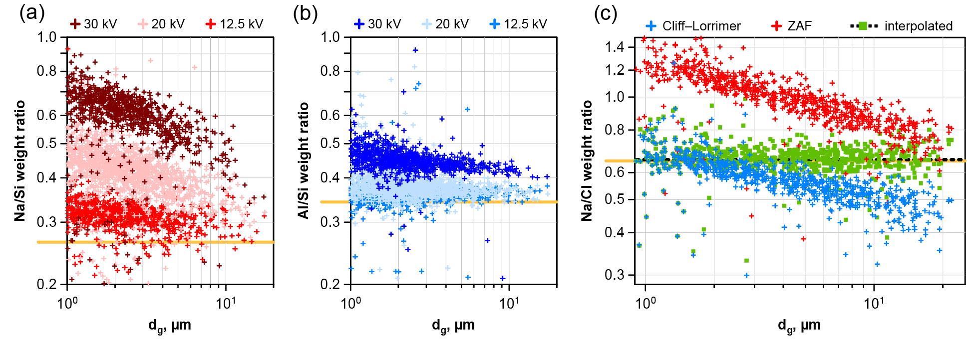
Figure 1 Comparison of element weight ratios for albite and sodium chloride powder as function of particle size. The nominal ratios for the compounds are shown as orange lines. (a, b)  Albite ratios as function of acceleration voltage with ZAF correction. (c) Sodium chloride ratio at 20 kV acceleration voltage, corrected by the methods Cliff–Lorrimer, ZAF and interpolated. The linear regression of the interpolated correction is shown as black striped line.

2.3.1 Quantification of elemental composition

Fully quantitative results in EDX analysis can only be achieved under specific sample conditions. When the composition of an analyzed spot is derived from an X-ray spectrum, the sample geometry has to be considered. Besides assuming perfect smoothness and homogeneity, either infinite sample depth (i.e., significantly larger than the interaction volume of a few µm) or presence of an infinitely thin film are commonly assumed. In the former case, a “ZAF” correction can be applied (Trincavelli et al., 2014), in the latter for example the Cliff–Lorimer method (Cliff and Lorimer, 1975). However, for particles these assumptions and the resulting quantifications are not valid, as shown by Laskin et al. (2006) in their Fig. 3. To overcome this problem, several standard-less techniques can be applied (Trincavelli et al., 2014), for example, a Monte Carlo simulation of the interaction volume can be used (Ro et al., 2003). Alternatively, particle ZAF algorithms can be applied at least for larger particles with diameters above 1 µm (Armstrong, 1991; Weinbruch et al., 1997). However, in the present work, an approach with less computational cost is applied. First, on the measurement side, a lower acceleration voltage, 12.5 kV instead of 20 kV in comparative studies, eases the particle morphology problem. The Fig. 1a and b show, for an albite standard, the Na ∕ Si and Al ∕ Si ratios, demonstrating the impact of different acceleration voltages on the quantification. Also, it is obvious that the problem is more pronounced for a higher difference in the energies of the characteristic peaks used for quantification. Second, on the data analysis side, by combining the mentioned correction methods as function of particle size, a higher accuracy in quantification can be achieved. In principle, particles smaller than a limit size are considered as thin films and particles larger than a second limit are considered to be of infinite depth. Between the limiting sizes, values are interpolated. To determine the best interpolation method, samples with well-known composition (sodium chloride, albite) were milled to obtain particle standards with sizes between 1 and 30 µm. Particles were dispersed in clean air, re-deposited on the same sampling substrate and analyzed like described above. Several non-linear interpolation schemes were tested; the best results were obtained with the following equation:

$$\begin{array}{}\text{(4)}& {\displaystyle }\langle X\rangle =\left\{\begin{array}{ll}{X}_{\mathrm{CL}}& d_{\mathrm{g}}\le d_{\mathrm{l}}\\ X_{\mathrm{CL}}+\left(X_{\mathrm{ZAF}}-X_{\mathrm{CL}}\right){\displaystyle \frac{\log (d_{\mathrm{g}}/d_{\mathrm{l}})}{\log (d_{\mathrm{u}}/d_{\mathrm{l}})}}& d_{\mathrm{l}}<d_{\mathrm{g}}\le d_{\mathrm{u}}\\ X_{\mathrm{ZAF}}& d_{\mathrm{g}}>d_{\mathrm{u}}\end{array}\right.,\end{array}$$

where 〈X〉 is the corrected concentration of a particular element in the beam interaction volume, X_CL the element concentration determined by the Cliff–Lorrimer method, X_ZAF the element concentration determined by the ZAF method, d_l=1.5 µm the lower interpolation range size limit, d_u=30 µm the upper interpolation range size limit.

Note that the concentrations are always normalized to 100 % of the beam interaction volume. This can include not only the particle, but also the substrate. For this reason, the substrate was chosen to be composed as differently as possible to all expected particle compositions. The correction is identical for atomic and mass concentrations; in the present paper, atomic concentrations are used unless otherwise specified.

The result of the correction as function of particle size is shown in Fig. 1c for 20 kV as demonstration (at 12.5 kV as used for the sample analyses, the problems are obviously less pronounced). It becomes clearly visible that the accuracy of the quantification is strongly improved, while the remaining uncertainty originates mainly from the particle to particle variation. This uncertainty depends on the noise in the analysis system, but is also related to particle surface morphology and its variability. The latter affects the X-ray signal mainly by unknown absorption path lengths, particularly for the lighter elements, as illustrated by Fletcher et al. (2011).

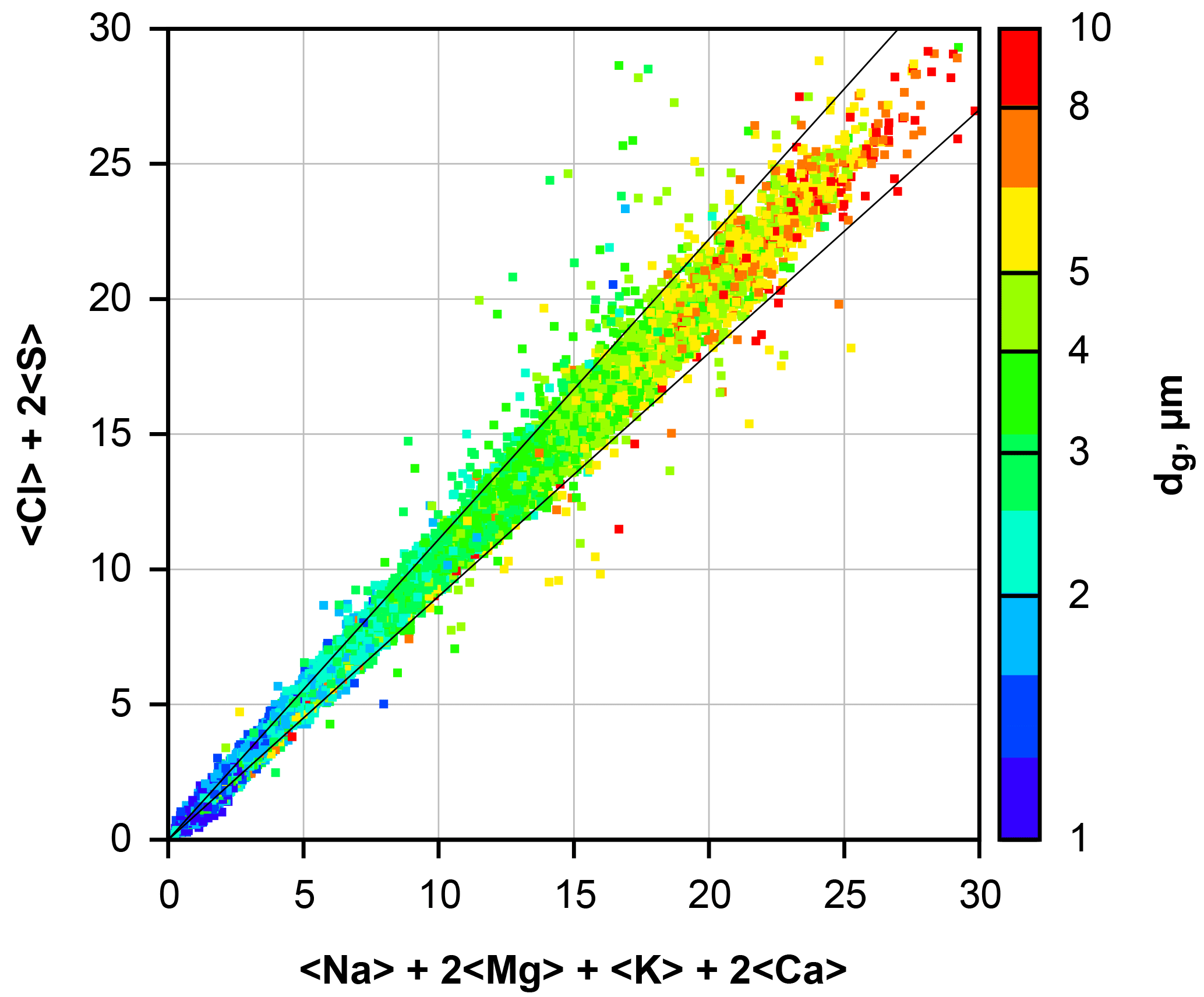
Figure 2 Calculated ion balance for all beam interaction volumes containing particles dominated by Na and Cl. Particles were collected by the DPDS. The axes are scaled in arbitrary units of percent × unit charges. Smaller particles yield smaller values as they only fill a fraction of the beam interaction volume. Particle size is color-coded; note that all particles between 0.6 and 1 µm in size are shown as blue, and between 10 and 25 µm as red. The black diagonal lines show the 10 % deviation cone.

Application to a sample of atmospheric particles is shown in Fig. 2. Particles dominated by Na and Cl were selected from all DPDS samples, and the positive and negative ion contributions were calculated for each particle from the determined concentration. It becomes obvious that for a wide size range the applied correction works well and thus produces unbiased relative concentrations for the considered elements. The outliers may occur due to noise, the negligence of C, N and O compounds or an internal mixture of sea salt with dust (e.g., NaAlSi₃O₈, FeS).

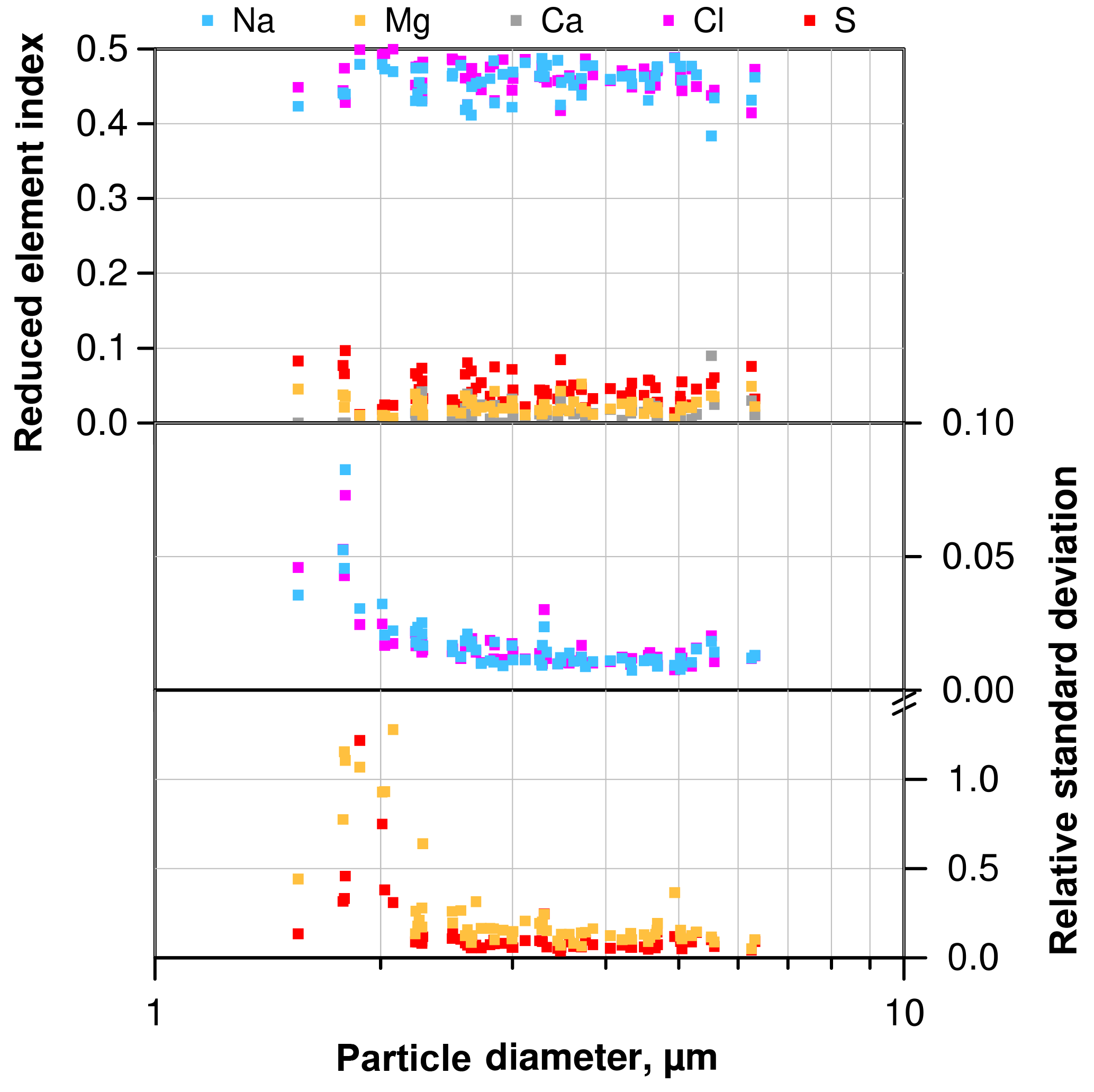
Figure 3 Mean element index only using Na, Mg, S, Cl and Ca for normalization, and according standard deviation (1σ) for NaCl-dominated particles from a typical atmospheric sample as function of particle size. Note that relative standard deviation for Ca is not shown due to frequent values below the detection limit.

2.3.2 Analytical measurement errors

A typical deposition sample (collected between 21 June 2013, 13:46 and 22 June, 15:02, LT) was analyzed 29 times with a signal collection time per particle of 16 s. The same 300 particles were analyzed each time. For illustration of the typical precision, the particles consisting mainly of Na and Cl were selected. Figure 3 illustrates the average composition and standard deviation (1σ) for each particle. The average values show a typical behavior for atmospheric sea salt with a slightly depleted Cl and enriched S concentration (e.g., McInnes et al., 1994). The precision, shown as relative standard deviation, increases with particle size. This is caused by the increasing amount of material contributing to the particle's signal up to a point at about 3 µm particles, from which the beam excitation volume is completely inside the particle. For the major compounds, the precision is in the range of 2 % relative standard deviation. For minor compounds, it is between 10 % and 20 % for particles 3 µm and larger, but can exceed 100 % for the smallest ones. The latter high uncertainties could be decreased with suitable working conditions (magnification, measurement time), but are not the focus of the present paper.

The uncertainty in particle diameter also depends on its size. For particles with a 2 µm diameter, the relative standard deviation is about 1.5 % decreasing to less than 1 % for particles larger than 3 µm. This is in the same range as the systematic accuracy of SEM (1 %–2 %).

2.3.3 Particle classification, relative ion balance and feldspar abundance

For assessing the abundances and counting statistics of certain particle types, the particles were classified into different groups and classes. Based on the element index and additional elemental ratios, a set of rules used in former mineral dust investigations in a marine environment was applied.For details, refer to Kandler et al. (2011a).

In addition, a relative ion balance is defined for single particles as follows:

$$\begin{array}{}\text{(5)}& {\displaystyle }{\mathrm{IB}}_{\mathrm{rel}}={\displaystyle \frac{\langle \mathrm{Na}\rangle +\mathrm{2}\langle \mathrm{Mg}\rangle +\langle \mathrm{K}\rangle +\mathrm{2}\langle \mathrm{Ca}\rangle -\langle \mathrm{Cl}\rangle -\mathrm{2}\langle \mathrm{S}\rangle }{\langle \mathrm{Na}\rangle +\mathrm{2}\langle \mathrm{Mg}\rangle +\langle \mathrm{K}\rangle +\mathrm{2}\langle \mathrm{Ca}\rangle +\langle \mathrm{Cl}\rangle +\mathrm{2}\langle \mathrm{S}\rangle }}.\end{array}$$

A positive relative ion balance, i.e., an excess of positive ions, would indicate an undetected presence of negative ions like ${\mathrm{NO}}_{\mathrm{3}}^{-}$ or ${\mathrm{CO}}_{\mathrm{3}}^{\mathrm{2}-}$, a negative one such of H⁺ or ${\mathrm{NH}}_{\mathrm{3}}^{+}$, which all can not be (reliably) quantified by EDX. The relative ion balance is calculated only for particles classified into the soluble sulfate or sea salt classes.

For the description of feldspar abundance, we define two index values, showing the vicinity for a single particle to pure feldspar or pure K-feldspar composition. These feldspar indices regard the overall contribution of feldspar-specific elements to the particle and the specific Al ∕ Si as well as alkali ∕ Si or K ∕ Si ratios. Measurements based on mineral dust generated from pure granite, i.e., dust practically free of clay minerals, have shown that a threshold value of 0.80 is suitable to distinguish between pure feldspar grains and other silicates. Details of the index calculation are given in the Supplement in Sect. S1. Note that aggregated particles consisting of feldspar and, for example, clay minerals, quartz or soluble species would not be classified as feldspar.

2.3.4 Estimation of the dust contribution to each single particle in a dust–sea salt–sulfate mixture and the size of the according dust inclusion

Sampling was performed in a region where locally emitted sea salt aerosol and other soluble species are mixed with long-range transported mineral dust. In particular, as the mineral dust contribution is of special interest, disentangling the particle populations and considering them separately is an important task.

To calculate the size of a dust inclusion and the according volume fraction for an internally mixed particle from the chemical composition, the different elemental contributions have to be attributed to the dust or non-dust component. This analysis is restricted in the present work to the major compounds. For Al, Si, P, Ti and Fe it can be safely assumed that they belong to a dust component (i.e., an inorganic, thermally stable, oxidized, non-carbonaceous compound), and S and Cl can be attributed to the non-dust component. However, Na, Mg, K and Ca are ambiguous and can be present in fractions. Therefore, a model is needed to estimate the contribution of the ambiguous elements from the dust and non-dust component based on the single particle chemical composition.

A problem arises here from the error in chemical quantification due to matrix composition and particle geometry. While the correction outlined in Sect. 2.3.1 adjusts the quantification accuracy of the average particle composition, for single particles – because of their unknown geometry and surface orientation angles – a considerable error in element quantification can still occur. In particular, a bias between lighter and heavier elements can be introduced by unaccounted X-ray absorption, which can lead to under- as well as overestimation of the relative contribution of light elements (Fletcher et al., 2011). As for the present aerosol, the major cations (Na⁺, Mg²⁺) are light in comparison to the major anions (Cl⁻, S of ${\mathrm{SO}}_{\mathrm{4}}^{\mathrm{2}-}$), a quantification bias will lead to an error in component attribution. Particularly, an overestimation of the light elements will yield, by attribution of the ion balance excess to the dust component, to an overestimation of the dust contribution. Therefore, two model pathways are applied: an upper limit estimate, where a possibly overestimated fraction of the ambiguous elements is attributed to the dust component, and a lower limit estimate, where all ambiguous elements are attributed to the non-dust component. Details on the procedure are given in Sect. S2 in the Supplement.

The model outlined here may suffer from systematic errors.

1. In the presence of larger amount of nitrate and ammonium or organics, the dust contribution will be overestimated, as the regarded composition is fitted to the apparent particle volume. However, on Barbados the concentration of these compounds is usually small in comparison to the dust (Lepple and Brine, 1976; Savoie et al., 1992; Eglinton et al., 2002; Prospero and Arimoto, 2009; Zamora et al., 2011).

2. The density values are averages for the assumed components, and the real density of a particle may be smaller or larger. However, the density range for the components in question is small (dust: 2300 to 3000 kg m⁻³; non-dust: 1800 to 2600 kg m⁻³ at maximum), so the error is considered to be less than 10 %.

3. The mass contribution is estimated by ion charge balances. If for the ambiguous elements an inhomogeneous distribution of univalent and bivalent elements exists (e.g., univalent as with Na favoring the non-dust component and bivalent as with Ca favoring the dust component), an error of less than 5 % in diameter can occur. With an assumption of 5 % iron content in dust, the maximum error due to the Fe³⁺ assumption is less than 0.2 % in diameter.

The upper and lower estimates yield diameters, which differ for the dust core diameter on average by 25 %; for 75 % of the particles the difference is less than a factor of two. From the analytical errors in ratios for major compounds (less than 10 % systematically and 6 % repetition uncertainty), an dust core size uncertainty of about 6 % is estimated, as long as the core is larger than 10 % of the particle. An overall analytical uncertainty of 15 % relative core size is estimated. In conjunction with the upper or lower limit estimates, an overall core size error of 25 % is considered appropriate.

Estimation of a geometrical iron availability index

Iron bioavailability in general is depending on different chemical and microphysical parameters as well as residence time in chemically aggressive environments (Shi et al., 2011a, 2012), e.g., at low pH values under influence of sulfuric or nitric acid. If considering a homogeneous iron distribution in larger and smaller particles, it seems plausible that the distance to the surface, thus the surface to volume ratio, should have an impact on the short-term iron accessibility (e.g., Baker and Jickells, 2006; Shi et al., 2011b). Therefore, as a first order estimate we define a geometrical surface iron availability index SIAI (after virtual dissolution of the soluble compounds) as follows:

$$\begin{array}{}\text{(6)}& {\displaystyle }\mathrm{SIAI}={\displaystyle \frac{{\mathrm{Fe}}_{\mathrm{oxide}}}{m_{\mathrm{dust}}}}\mathit{\pi }{d}_{\mathrm{v},\mathrm{dust}}^{\mathrm{2}},\end{array}$$

with Fe_oxide iron oxide mass estimated as Fe₂O₃, m_dust the dust elements oxide mass (refer to Sect. S2 in the Supplement), d_v, dust the volume-equivalent diameter of the particle dust fraction.

It should be noted that this approach is of a geometrical nature only and does not take into account environmental factors like pH and presence of ligands.

2.3.5 Statistical uncertainty of total volumes and masses and relative number abundances from single particle measurements

When assessing the uncertainty of values based on counted occurrences, frequently the counting statistics are assumed to follow a Poisson distribution. However, when calculating total aerosol masses or volumes, besides the measurement errors in particular the (usually few) large particles can introduce a considerable statistical uncertainty, which is not necessarily accounted for by the distribution assumption. Therefore, estimates of the statistical uncertainty based on single particle counts for an a priori unknown frequency distribution (i.e., the counting frequency distribution modified by the also unknown particle size distribution), either require reasonable assumptions or distribution-independent estimators. In the present work, the uncertainty is estimated by a bootstrap approach with a Monte Carlo approximation (Efron, 1979). For the bootstrap approach, a considerable number of data replications are necessary (Carpenter and Bithell, 2000; Pattengale et al., 2010). As for the actual number, different recommendations exist, with more than 1000 being among the most common (Carpenter and Bithell, 2000). As higher numbers lead to smaller errors in the uncertainty estimate, 10 000 replications for each sample were performed in the present work. A comparison of the results of the generally robust bootstrap approach (Efron, 2003) to a more simple approach, where the counting statistics is assumed to follow a Poisson distribution, is given in Sect. S3 of the Supplement.

For the assessment of the confidence interval of relative counting abundances, a confidence interval based on a binomial distribution is used as an estimate (Agresti and Coull, 1998), i.e., for a relative number abundance of a certain particle type class r the two-sided 95 % confidence interval is approximated (Hartung et al., 2005).

2.4 Collection efficiency and deposition velocity relating atmospheric concentrations to deposition rates

2.4.1 Determining the size distributions from the free-wing impactor measurements

Obtaining the atmospheric size distribution and representative contributions of particle populations with different hygroscopicity from the FWI requires two corrections. These corrections are applied to each single particle as a function of its size and composition and the thermodynamic and humidity conditions during sampling. First, a window correction is applied, accounting for the exclusion of particles at the analysis image border (Kandler et al., 2009). Second, the FWI collection efficiency is corrected. For the detailed formalism, refer to Sect. S4 of the Supplement.

Potential systematic error sources for this calculation are mainly the uncertainty in collection efficiency, given the considerable spread in data points in the according literature (Golovin and Putnam, 1962; May and Clifford, 1967), and any bias in particle size.

2.4.2 Determining the airborne size distributions from the sedimentation sampler measurements

Sampling efficiency considerations are also necessary for the sedimentation sampler. For the supermicron particle size range sedimentation and turbulent impaction dominate the particle deposition velocity (as for example illustrated by Piskunov, 2009).

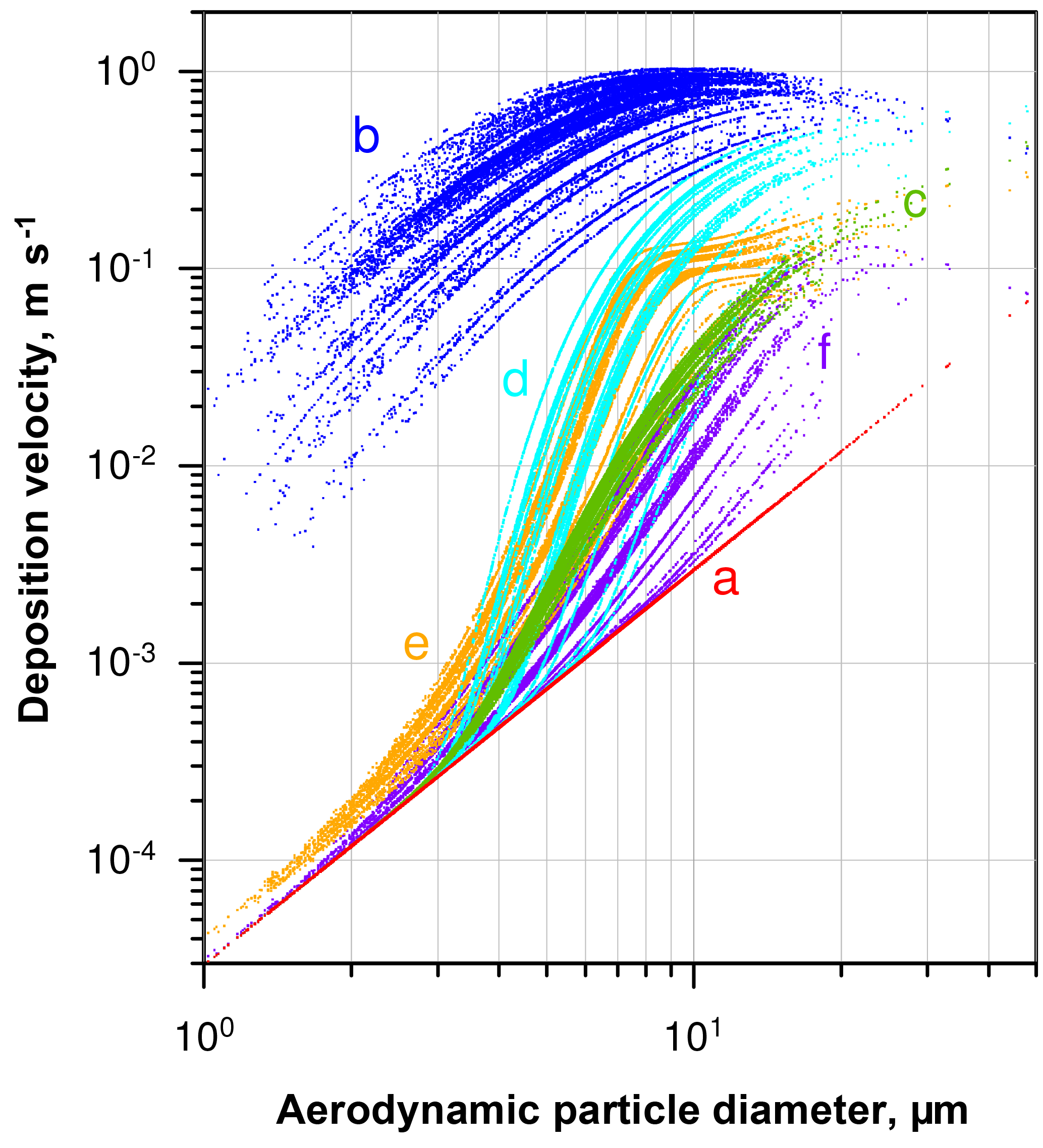
Figure 4 Deposition velocity to a smooth surface calculated by different deposition models for the samples of 2013, taking into account the ambient thermodynamic conditions and the particle composition. (a) Stokes settling; (b) Noll et al. (2001); (c) Noll and Fang (1989); (d) Aluko and Noll (2006); (e) Piskunov (2009); (f) Wagner and Leith (2001).

A variety of models estimating the particle deposition speed were published (Sehmel, 1973; Slinn and Slinn, 1980; Noll et al., 2001; Wagner and Leith, 2001; Aluko and Noll, 2006; Piskunov, 2009; Petroff and Zhang, 2010). They yield considerable different results, possibly due to negligence of unaccounted forces (e.g., Lai and Nazaroff, 2005), the way of determining the relevant friction velocity, or other model assumptions. For the present work, the formalism of Piskunov (2009) was selected, as it derives the deposition velocity from physical principles instead of parameterizing a specific measurement setup. Details of the calculation procedure are given in Sect. S5 of the Supplement. The deposition velocity calculated by different formalisms for a series of deposition samples is shown in Fig. 4.

The spread in deposition velocity for each model is caused mainly by the different wind speeds during exposure, but also by the variation in relative humidity and, to a lesser extent, by other thermodynamic conditions. However, it becomes strikingly obvious that in the size range where most of the atmospheric dust deposition occurs, i.e., between 2 and 50 µm in diameter on Barbados (Mahowald et al., 2014; van der Does et al., 2016), the models disagree by more than 2 orders of magnitude. Besides the uncertainty derived from selection of a particular model, the sphericity assumption and the related drag effects may lead to a bias in deposition flux, most probably mainly influencing the turbulent deposition regime around a 10 µm particle diameter. An additional measurement bias might be introduced by the parallelism assumption underlying all the stable boundary layer calculations, i.e., that the air flow must be parallel to the plate. While the vertical component of the wind speed under atmospheric conditions is usually small in comparison to the horizontal ones, “inlet” losses might still occur due to small non-parallel components. These inlet losses are expected to mainly affect the largest particles sizes.

2.4.3 Impactor inlets

The impactor sampler was used with two types of inlets. For particles larger than approximately 2.5 µm in aerodynamic diameter, a pseudo-isoaxial inlet orientation with sub-isokinetic sampling was used. Smaller particles were collected with an omnidirectional inlet. As particles were analyzed separately for each size class, the inlet efficiency does not play a primary role for the results, but it must still be considered. Literature on an accurate estimation of inlet transmission for a ratio between ambient wind speed and impactor inlet flow velocity in the range of 100:1 does not exist. However, from Paik and Vincent (2002) and Hangal and Willeke (1990) in conjunction with the observation of Li and Lundgren (2002) regarding the applicability of thin walled nozzle formulas to blunt samplers, the following may be concluded.

• a.

  Particles larger than 2.5 µm in aerodynamic diameter would be increasingly enriched with increasing particle sizes. Enrichment factors for thin-walled nozzles would be in the range of 2–4 for 10 µm particles and 20–50 for 100 µm particles. As the sampler had a blunt inlet, the actual enrichment factors are probably considerably lower.

• b.

  Particles smaller than 2.5 µm would be comparatively unbiased at low Stokes numbers; see also Wen and Ingham (2000).

For a dry aerosol, these size-selective inlet losses would not considerably bias the relative chemical composition. In the present humid environment with partly soluble species, though, it can lead to an overestimation of non-hygroscopic species for particle sizes in the vicinity of the inlet cut-off if the hygroscopic growth is not explicitly considered. The problem is somewhat diminished by the fact that by water-absorption the density of the particles decreases and, consequently, the Stokes number increases only sub-proportionally to the square of the particle diameter. Nevertheless, the hygroscopic growth should be explicitly accounted for. Therefore, the hygroscopicity model is applied based on the measured geometric diameter and chemical composition, and ambient chemical compositions are computed.

2.5 Modeling deposition statistics and artifacts of mixing state

When particles are deposited to a substrate, they might touch each other and form an internal mixture, which is not representative for the atmosphere. While the lower limit of coincidental internal particle mixture on a substrate is easily defined – it equals the ratio of the area covered by particles to the total analyses area for an infinitesimally small depositing particle – the assessment is much more complex for larger particles following a wide size distribution function.

Therefore, in the first step the deposition process was simulated by a series of Monte Carlo models. For input, the average size distribution measured at Cape Verde (Kandler et al., 2011b), hereafter CV-ground, and the median one measured airborne for aged dust (Weinzierl et al., 2011), hereafter CV-air, were used. These size distributions mainly differ in the concentration of supermicron particles. The deposition velocity formulation after Piskunov (2009) was used. The modeled deposition area is 5 mm × 5 mm, meteorological conditions were assumed as totally dry, 20 ^∘C, with sea level pressure and a friction velocity of 0.2 m s⁻¹. Particles were virtually dropped onto the deposition surface until either a certain fractional area coverage by particles or a simulated deposition time limit was reached. The 18 different area coverages were simulated for a two component external mixture (particle density 2200 kg m⁻³) with components number ratios of 50 %∕50 %, 75 %∕5 %, 90 %∕10 %, 95 %∕5 %, 97 %∕3 % and 99 %∕1 % for CV-ground, and nine area coverages with number ratios of 50 %/50%, 90 %∕10 % and 99 %∕1 % for CV-air. Each model was run 1000 times (200 times in case of 0.1 and larger fraction area coverages) to assess the statistical uncertainty. In a second series, for CV-ground a tricomponent external mixture of sodium sulfate (particle density 1770 kg m⁻³), dust (2700 kg m⁻³) and sea salt (2170 kg m⁻³) was used as input. The size-dependent component number contributions were taken from measurements at Cape Verde (Schladitz et al., 2011). After the simulated deposition, particle agglomerates on the substrate with touching contours were merged into a new particle with the sum of the volumes and proportionate chemical composition.

To investigate the relevance of mixing artifacts caused by particle sampling, the sensitivity of SEM/EDX analysis has to be considered. Internal mixtures can be only detected by SEM/EDX if the minor component exceeds the limit of detection. At an acceleration voltage of 12.5 kV, the primary X-ray excitation volume is in the range of 0.5 to 1.5 µm in diameter, depending on the matrix elements (Goldstein et al., 2003). As we consider mainly supermicron particles, the excitation volume is expected to be mainly inside the particles. According to our experience an X-ray peak becomes detectable at about 0.3 % concentration. Therefore, a 1 % contribution of an element to the particle volume will definitely be detectable. Thus, a particle containing more than 1 % material from another particle type is considered as detectable mixture in the model. A particle containing more than 20 % is denominated as strong internal mixture. Note that for smaller particles, when the excitation volume would extend into the substrate, larger contributions to the particle volume would be required.

Besides these fundamental considerations, in the second step, a mixing model was applied to each sample, based on its measured composition. Random particles were virtually selected from the pure components of the measured set of particles and placed at random positions inside a virtual area with the same size as the one analyzed in SEM/EDX, until the same area coverage as of the real sample was reached. Internal mixtures artificially produced on the substrate were counted if their mixing would have been detected by SEM/EDX applying the rules for mixed particle classification. This process was repeated 10 000 times. The upper 95 % confidence interval limit of mixtures modeled by the Monte Carlo simulation was considered as the limit of detection for internal mixtures, and the median of the produced mixtures was regarded as systematic error and was subtracted from the mixtures detected in the real samples.

In the third step, the single mixing probability (SMP) for each binary pure compound combination was calculated by selecting 100 000 random pure-composition particles from the measured data set for each sample, mixing them virtually and determining whether they would be detected as mixed. This was carried out once without any size restrictions and a second time only selecting particles no more than a factor of 3 different in size. The latter was done to account for the fact that in a turbulent environment and in the regarded size range, the collision efficiency is highest for particles of similar size (Pinsky et al., 1999; Wang et al., 2005).

2.5.1 Simulating particle mixtures due to longer exposure times

While in the modeling section particles are assumed to be spherical, this is typically not the case for natural aerosol like mineral dust particles. Therefore, a second approach based on particle images was used to estimate the effect of internal particle mixture on the substrate, i.e., taking into account the real particle shapes. Due to the large number of images required, this approach could only be used for assessing the size statistics, but not for the chemical composition. All segmented images of each deposition sample were subject to particle size analysis. In following steps, a number of 2, 3, 5, 10, 15, or 20 segmented images of the same sample were combined into a single image, simulating an extension of exposure time by the according factor. This approach inherently assumes a constant size distribution during exposure and a random particle deposition. The resulting images were then subject to the same particle analysis, yielding apparent size distributions after a coincidental mixing. In contrast to the pure modeling approach, here the true size distribution is not known because even the lowest coverage samples might contain internal mixtures. Certainly though, the lowest coverage sample is closest to the true size distribution and thus will be used as reference.

3 Results and discussion

3.1 Uncertainty of measurements for the new collection techniques and determination of mixing state

3.1.1 Area homogeneity of collected particles

Free-wing impactor (FWI)

To assess the homogeneity of particle distribution, for each sample, the center 80 mm² (about 65 % of the total sample area) were scanned with approximately 1000 SEM images (approximately one-third coverage), and the average particle density was determined for each mm² as function of d_g. For particles between 4 µm and 8 µm in diameter (see Fig. S5 in the Supplement) no systematic bias in particle density is visible, except for a slight enhancement toward the borders in a few cases. The remaining variability probably remains linked to statistical uncertainty and surface defects interpreted as particles by the automatic segmentation algorithm. However, the density variations between each mm² remain below a factor of 2. As commonly 20 to 100 mm² are analyzed, the inhomogeneity can be regarded as minor error. For larger particles, the uncertainty due to counting statistics becomes dominant.

Dry particle deposition sampler (DPDS)

Similar to above, the DPDS deposition density homogeneity was assessed, but in this case nearly all of the central 80 mm² were scanned. In about half of the samples, a crescent-shaped density gradient can be observed (see Fig. S6 in the Supplement). This gradient most probably originates from a stationary wave introduced by the recession of the sample substrate slightly below the primary plane of the DPDS. Depending on the analysis location, a bias in the range of factor 2 to 3 in deposited particle number can occur. Therefore, the fields of analysis for the chemical composition and size distribution discussion below were homogeneously distributed over the sample surface at a regular distance. For larger particles the uncertainty due to counting statistics also becomes dominant with the DPDS.

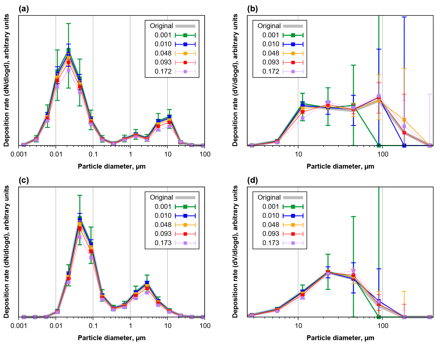
Figure 5 Number (a, c) and volume size distributions (b, d) of deposition rates as function of projected area in diameter, modeled for Cape Verde aerosol as derived from a 5 mm × 5 mm analysis field. Panels (a) and (b) are based on CV-ground, panels (c) and (d) on CV-air size distributions. The grey curve shows the original size distribution of deposited particles, the colored points with whiskers give median and central 95 % quantile of 1000 repetitions (200 for 0.093 and 0.172/0.173) for distributions calculated from samples with different area fractions covered by particles.

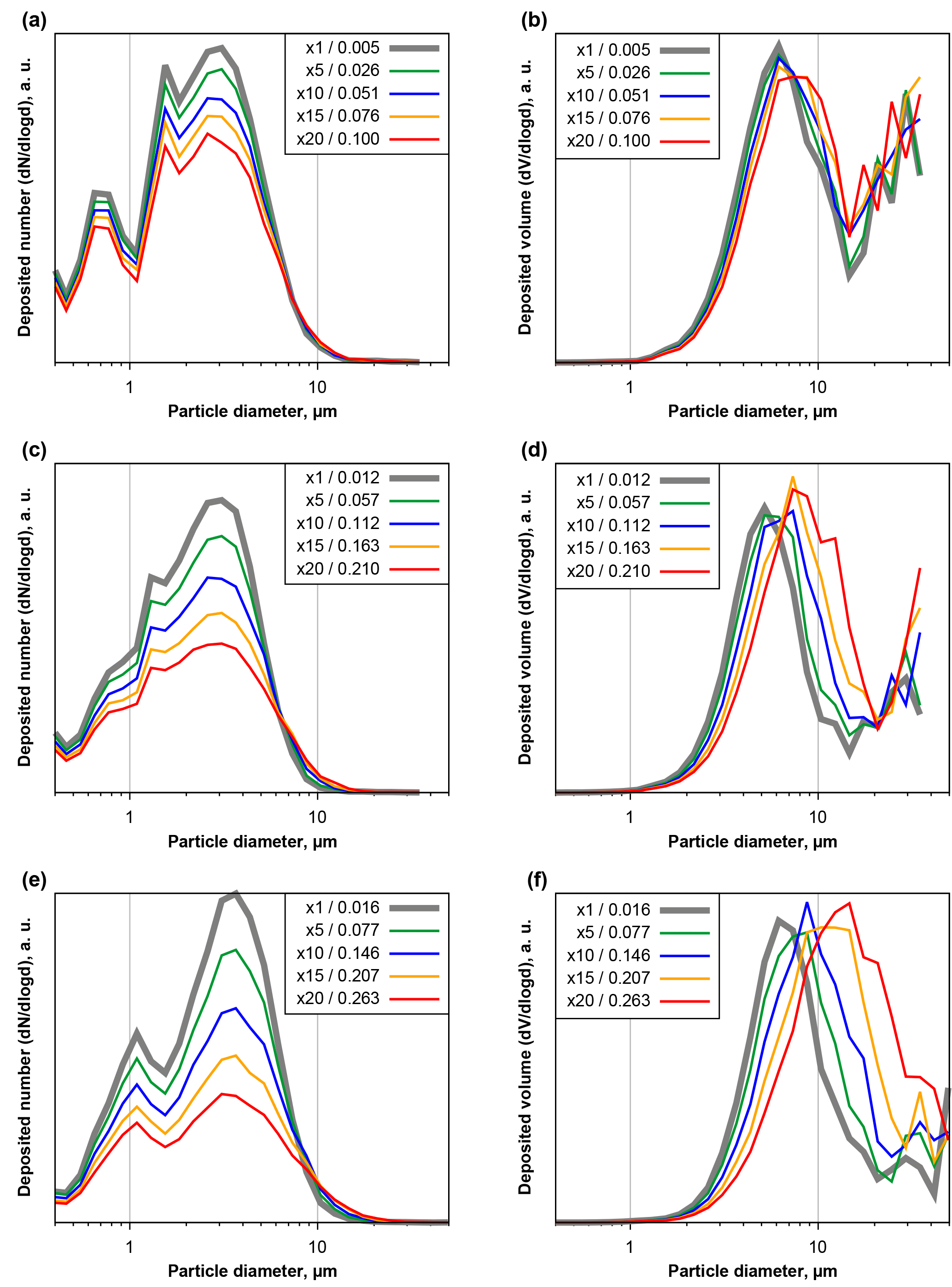
Figure 6 Number (a, c, e) and volume size distributions (b, d, f) of deposited particles measured at Ragged Point and extrapolated change as function of particle projected area diameter and area coverage fraction, simulating a longer exposure time. Plots are given for low (a, b), medium (c, d) and high (e, f) base coverages. Different colors show different factors of exposure increase (5×, 10×, 15×, 20×). Resulting coverage fractions are given in the figure keys.

3.1.2 Impact of area coverage and counting statistics on size distribution and total volume

Figure 5 shows the apparent number and volume size distributions of particles deposited from aerosols with CV-ground (a, b) or CV-air (c, d) size distribution for different area coverages, equaling different exposure times. As it is to be expected, for short exposure times there is a considerable counting error, which decreases to less than 10 % for the smaller particles at area coverages of 0.01 and higher. In the median, no particle larger than 50 µm would be detected in deposition area for area coverages smaller than 0.0025, and more than 0.005 is necessary to collect more than 5 particles (not shown in graphs). As opposing trend there is a bias in size distribution towards lower concentrations and larger particles, which starts getting relevant at coverages of 0.1. This bias is introduced by the coincidental clumping, a second particle depositing on an already deposited one. As a result, for the given aerosol size distributions, an area coverage of 0.03 to 0.05 is most appropriate to get a size distribution influenced least by counting errors and sampling and mixing biases.

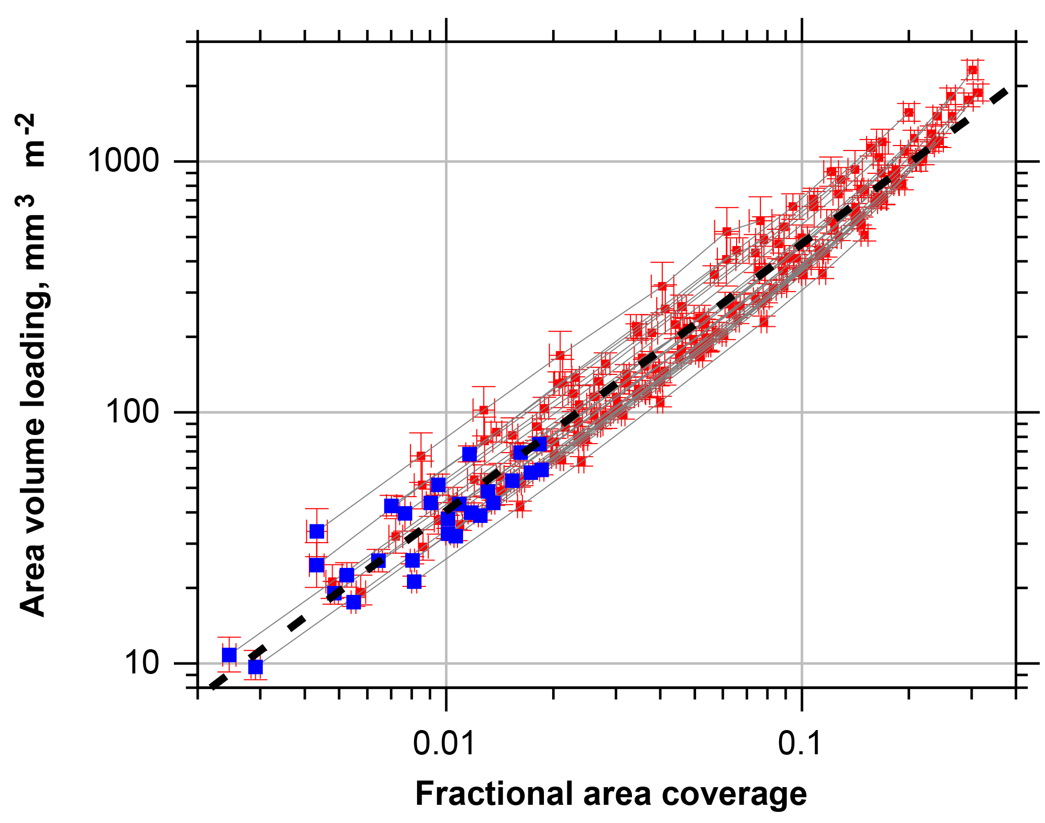
Figure 7 Particle volume per area calculated from single particle measurements as function of the fractional area coverage. Blue symbols denote the unmodified samples, red symbols the simulation of higher coverage by factors of 2, 3, 5, 10, 15 and 20. Error bars denote the two-sided 95 % confidence interval. The fit function shown as black dashed line is calculated as $y=\exp \left(a\ln \left(x\right)+b\right)$ ; $\left[y\right]={\mathrm{mm}}^{\mathrm{3}}{\mathrm{m}}^{-\mathrm{2}}$; $a=\mathrm{0.957}\pm \mathrm{0.041}$; $b=\mathrm{3.57}\pm \mathrm{0.06}$; x is the fractional area coverage.

Generally similar but more pronounced effects can be observed if the second approach, simulating longer exposure times by combining real microscope images, is used. Figure 6 shows three samples, low (a, b), medium (c, d) and high (e, f) area coverages, of the evolution of the size distribution due to simulated longer exposure times. In case of high dust deposition rates and long exposure times, particles smaller than 10 µm in diameter would be underestimated by a factor of more than 2, while larger particles would be considerably overrepresented. A shift in the modal diameter of 50 % towards a larger size could be the result. However, at the large end of the volume size distribution, counting statistics might considerably influence the total particle mass uncertainty, even at these long simulated exposure times.

If total mass deposition is estimated from the microscope images, one can set up a relation of total volume and apparent area coverage, which might serve as a quick estimate of total deposited particle mass (Fig. 7). If the result of the fit function is multiplied with an approximate particle density, the result gives the deposition in mg m⁻² with an uncertainty factor of 2. As expected, the fit function starts to underestimates the volume and mass for high area coverage.

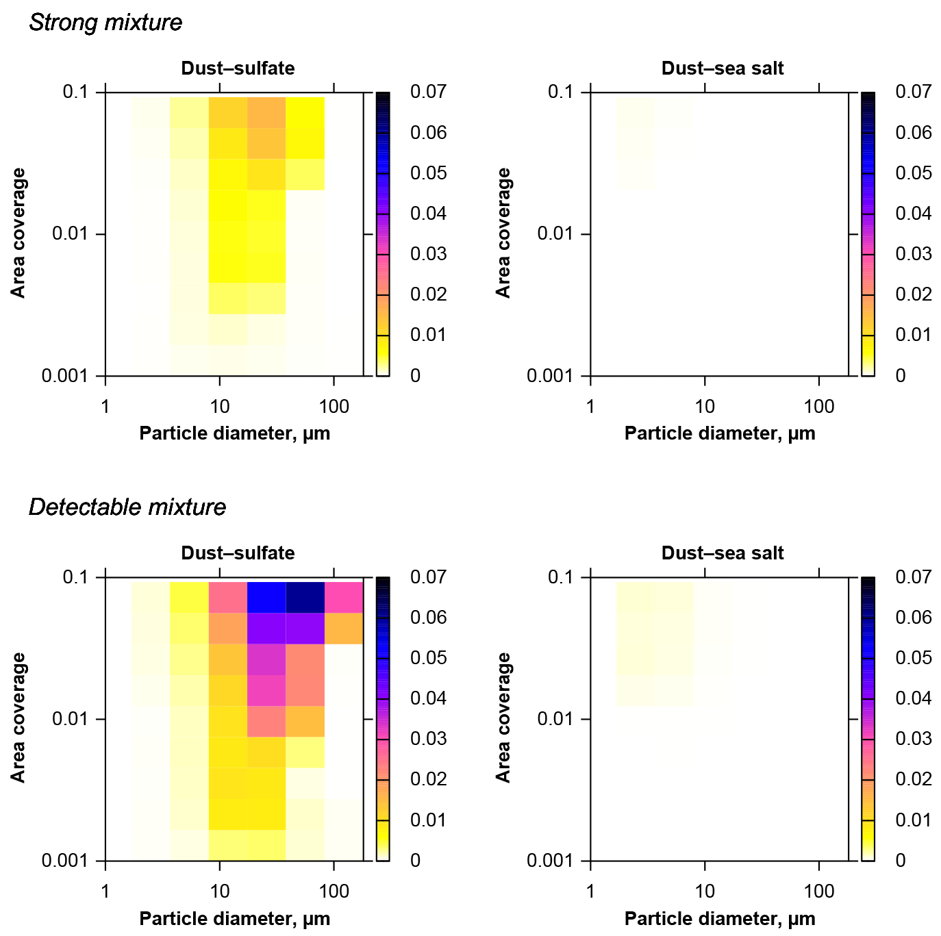
Figure 8 Upper 95 % quantile of the fractions of internally mixed particles due to coincidental mixing on the substrate (color scale), for a dust–sea salt–sulfate system with measured composition and CV-ground size distribution. Strong mixture refers to a minimum particle volume fraction of the other component of 20 %, detectable mixture refers to 1 %. Mixing compounds are given on top of each graph. Practically, sulfate–sea salt and ternary mixtures do not form coincidentally.

When calculating total mass/volume from small amounts of material, special attention has to be paid to the errors introduced by counting statistics. To assess the uncertainty, two size distributions were considered with different abundance of large particles. Using the CV-ground size distribution, we observe an uncertainty of a factor of 2 for the total mass (95 % two-sided confidence interval), when 3000 particles are counted, which are equivalent to 8 µg of mass. If only particles between 1 and 32 µm in diameter are regarded, a relative uncertainty of 20 % is achieved with 1500 particles. When analyzing about 100 µg of particle mass, the statistical error is in the range of 30 % mass in case of CV-ground size distribution and 15 % for CV-air. Table S3 in the Supplement gives more details for deposition simulation results based on a typical area, which would be used for automated single particle analysis. It can be concluded here that a minimum number of 5000 to 10 000 single particle measurements would be desirable to stabilize the total mass concentration in the range of 10 % uncertainty. As this number is usually not reached in SEM studies (e.g., Reid et al., 2003; Coz et al., 2009; Kandler et al., 2011a), additional attention should be paid to larger particles, e.g., by analyzing larger sample areas, to decrease the uncertainty in mass. Note that the same considerations, in principle, apply to bulk investigations, when only small amounts of mass are analyzed, but are not commonly stated.

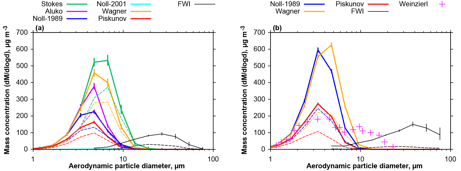
Figure 9 Average atmospheric mass size distribution densities derived from DPDS and FWI measurements. (a) The period from 10 to 15 July 2013; (b) and the period from 14 June to 8 July 2013. Different colors refer to different deposition velocity estimates as shown in Fig. 4. Solid lines refer to total mass concentrations, dashed ones to the dust mass estimated from the chemical composition (upper limit estimate). Error bars show the central 95 % confidence interval. Pink crosses show a size distribution measured in the Saharan Air Layer on 22 June 2013 (Weinzierl et al., 2017). Note that for particles smaller than 10 µm the FWI data may contain a considerable bias in calculation.

3.1.3 Amount of coincidental internal particle mixtures

When assessing the mixing state of particles from an offline single particle technique, coincidental internal particle mixture has to be taken into account. Higher area coverage, as to be expected, yields higher mixture probability. In particular, if components are present in equal abundances, mixing probabilities already become high for a covered area fraction of a few percent. As an example, Fig. S7 in the Supplement shows the upper 95 % confidence limit, i.e., the detection limit for mixtures, of apparent fractions of internally mixed particles for a two component system as function of source component ratio and area coverage for detectable strong internal mixtures (refer to Sect. 2.5; data are given also in the Supplement, Tables S4 and S5). No significant mixture for submicron particles occurs in these cases. Note also the different size maximum for strong vs. detectable mixture.

Applying the same model type based on the CV-ground size distribution to a ternary modal composition distribution of sulfate, sea salt and dust as described in Sect. 2.5, mixing probabilities for a specific atmospheric composition can be estimated (Fig. 8). It becomes instantly obvious that the mixing probabilities for this atmospherically more relevant aerosol model are much lower than in the homogeneous case. Mixtures between sulfate and sea salt as well as ternary mixture are absent. The relative fraction of internally mixed particles is lower by an order of magnitude. This can be explained by the fact that the defined relative detection limits of 20 % and 1 % restrict the detection of mixing to mixing partners not differing in size by more than a factor of 1.59 (strong mixing) and 4.6 (detectable mixing). However, because different aerosol types are mainly present in different size regimes here (Schladitz et al., 2011), the mixture can only be efficient for size ranges, where these component have an overlap. In general, mixture also increases with particle size.

It can be concluded that mixing studies for large particles are generally very difficult. Many particles need to be collected in total to ensure reliable counting statistics, which leads in consequence to high mixing probabilities. This issue is of less concern for particles smaller than 10 µm for the given size distributions and in cases where the aerosol has a strong dependence of composition on particle size. It also emphasizes that mixing studies should be accompanied by mixture modeling as performed here.

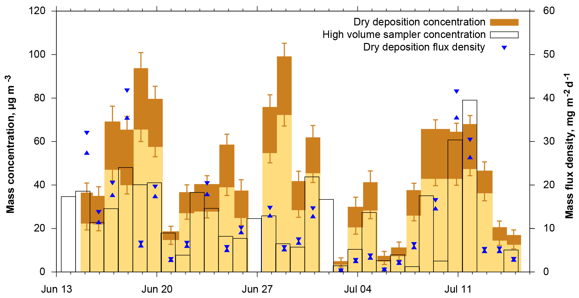
Figure 10 Dust mass concentration and flux density time series derived from DPDS compared to those obtained from a high-volume sampler (Kristensen et al., 2016). The darker brown bar shows the range from lower to upper estimate, the blue triangles the lower and upper estimate of dust deposition flux density. The date refers to the year 2013.

3.2 Field measurements – methodological aspect

3.2.1 Comparison of atmospheric size and volume concentrations

Using the FWI sampling efficiencies outlined in Sect. 2.4.1 and the DPDS deposition velocities from 2.4.2, one can calculate the atmospheric size distribution derived by the two techniques. Figure 9 shows the average size distributions for the post- and pre-storm periods based on different deposition velocity models for total and upper estimate dust mass concentrations. The lower dust estimate (not shown) exhibits qualitatively the same behavior. It is evident that there is a large discrepancy between the different models as well as between the DPDS and FWI measurements. The discrepancy is clearly larger than the statistical uncertainties. While the total mass median diameter derived from DPDS (Piskunov model) is around 5 µm in particle diameter, for the FWI it is approximately 25 µm. A dust size distribution measured in the Saharan Air Layer in 2.3 km altitude (computed from data shown by Weinzierl et al., 2017) contains the same mode around 4 µm in diameter, but shows a secondary maximum at 10 µm, which is not found by the ground-based measurements. It is interesting to note that these values get closer together when only the dust fraction is considered, indicating a connection of the discrepancy with the hygroscopic growth (e.g., growth or density misestimate). Three other reasons for the discrepancy might be an uncertain collection efficiency for the FWI, particle losses due to non-parallel flow for the DPDS, and non-parallel sampling times. The FWI has 50 % collection efficiency around 11 µm in particle aerodynamic diameter, so for smaller particles, the majority by far, the efficiency correction function may yield unrealistic values. The DPDS model assumptions require a well oriented flow. At high wind speeds, a non-zero angle of attack flow (from below) might lead to considerable particle losses for the larger particles. This might, for example, be caused by an increased boundary layer thickness over the lower plate. Such an angular flow was observed at the measurement site due to the cape orography. Finally, a discrepancy in sampling times (DPDS: approximately 1 day, FWI: approximately 1 h) may yield a bias. However, as similar differences are observed for all samples, the latter is most probably a minor aspect.

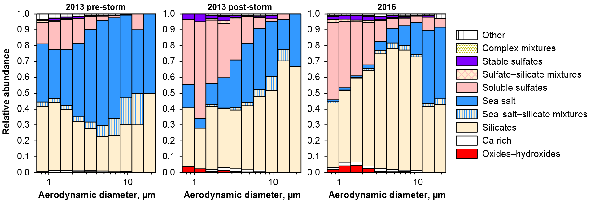
Figure 11 Size dependence of the relative number abundance of major particle types, as derived from single particle analysis of deposited aerosol.

Figure 12 (a) Box plot of daily mass deposition rate for total dust and dust-derived elements on Barbados for 2013 and 2016. (b) Cumulative mass deposition flux as function of aerodynamic particle diameter for dust and dust-derived elements. Note that for P and Ti in the latter plot two particles containing each more than 10 % of the total deposited mass have been removed from the data set.

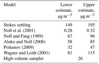
When total mass is calculated from deposition, it can be compared to dust concentration measurements with a high volume filter sampler. Figure 10 shows time series of mass concentrations measured by the high-volume sampler, estimated from dry deposition measurements as well as the raw dry deposition flux densities. For dry deposition, uncertainties derived from the lower or upper estimates as well as from counting statistics are shown. A few things can be learned from this data. With respect to the deposition model, the Piskunov model performs rather well. The average of the high-volume sampler mass concentration time series (see Table 1) is close to the lower estimate of the Piskunov model, while the higher estimate overestimates the mass concentration. The other models deviate considerably more, as to be expected from the deposition velocity differences (Fig. 4). The ratio of the mass concentration estimate to the mass flux density varies over slightly more than an order of magnitude, depending mainly on size distribution and wind conditions. High volume and deposition-estimated mass concentrations as well as the mass flux densities follow qualitatively the same pattern in showing low concentration and high concentration periods. However, the absolute numbers deviate significantly. For sub-periods, the correlation quality seems to be different. For example, starting from 21 June, the correlation of mass flux with high volume mass concentrations seems to be better than the one with deposition estimated concentrations; for the period before 21 June the situation is inverted. No direct link between the correlations and any meteorological variable was found, indicating that the deviations depend in part on erroneous assumptions in the model. For example, tuning other deposition velocity models by arbitrary factors can lead to a better agreement of actively and passively determined mass concentrations for this particular data set (Fig. S10 in the Supplement), but the data basis is too small for a robust tuning without physical backing. Moreover, disagreement might also be caused by physical measurement biases like unknown size-dependent inlet efficiency for the high-volume sampler or angular inflow for the DPDS.

Table 1 Average dust mass concentrations, estimated from deposited particle mass, applying various deposition models. Lower and upper refer to different dust fraction estimates (see Sect. 2.3.3).

3.3 Field measurements – atmospheric and aerosol aspects

3.3.1 Aerosol composition

Overall aerosol composition (i.e., the relative number abundance of the different particle groups) was measured by electron microscopy single particle analysis (Fig. 11). The relative abundance of soluble sulfate is highest for the smallest particle sizes, which is in good accordance with previous measurements in the eastern Atlantic Ocean (Kandler et al., 2011a). After the storm's passage, higher sulfate abundances, soluble as well as stable, are observed in 2013, which are similar to those observed in 2016. The sea salt abundance is higher for the pre-storm period in 2013, which is in agreement with the wind speeds observed (see below). In 2016, a much higher abundance of small Fe-rich particles (contained in the oxides/hydroxides class) is observed compared to the pre-storm period in 2013. For the post-storm period in 2013, minor amounts of these particles are visible.

Overall, an average dust deposition of 10 mg m⁻² d⁻¹ (range 0.5–47 mg m⁻² d⁻¹) is observed (Fig. 12). While a strict disambiguation can not be done for elements also found in sea salt, Al, Si, P, Ti and Fe are most likely derived from dust only and are thus also shown in the graph. On Barbados, Fe contributes 0.67 (0.01–3.3) mg m⁻² d⁻¹ to deposition, while phosphorous adds only 0.001 mg m⁻² d⁻¹; however, P is below the detection limit on two-thirds of the days. The cumulative size distribution shows that in particular P and Ti are located preferentially within smaller particles. Al, Si and Fe generally show a similar size distribution.

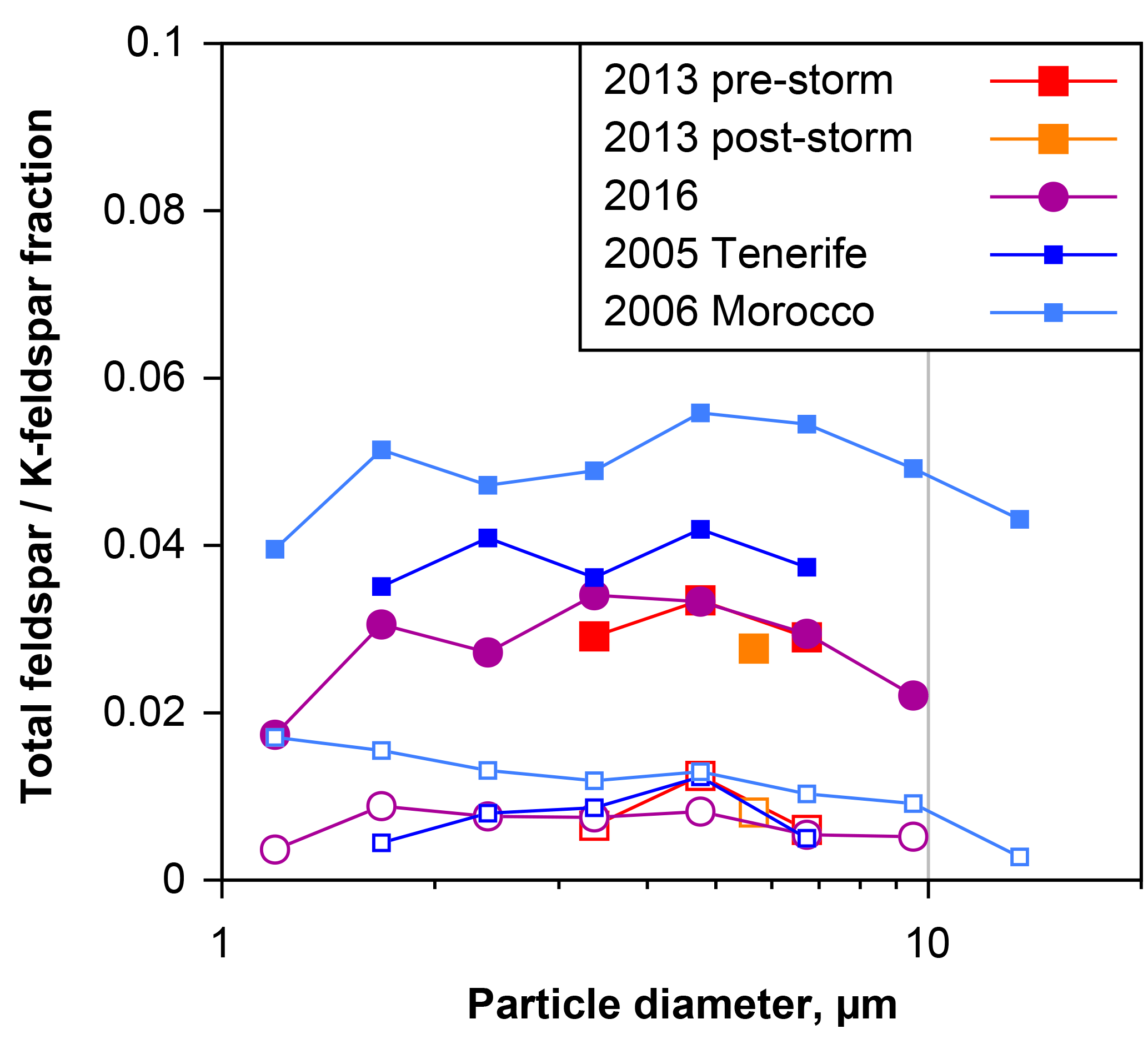
Figure 13 Number ratio of total feldspar (filled symbols) and K-feldspar (open symbols) to total silicate particles, as a function of particle aerodynamic diameter in dry deposition collected on Barbados. For comparison, data from Tenerife (Kandler et al., 2007) and Morocco (Kandler et al., 2009) are given. Only data points with less than 30 % relative counting error are shown.

Recently, the impact of mineral dust composition on clouds via the ice phase has attracted attention. Feldspar particles and in particular K-feldspars are discussed as most efficient ice nuclei (Atkinson et al., 2013; Augustin-Bauditz et al., 2014; Harrison et al., 2016). Therefore, Fig. 13 shows the total feldspar and K-feldspar number fractions with respect to all silicates as determined by the feldspar indices. In general, approximately 3 % of the silicates are pure feldspar particles and slightly less than 1 % K-feldspars. No significant variation is visible for the different periods and years on Barbados, whereas particles collected in Morocco (Kandler et al., 2009) showed slightly higher values. In this respect, the dust composition on Barbados is constant over time. Note that the bulk feldspar contents of the samples might be higher, as the applied technique only detects pure feldspar grains.

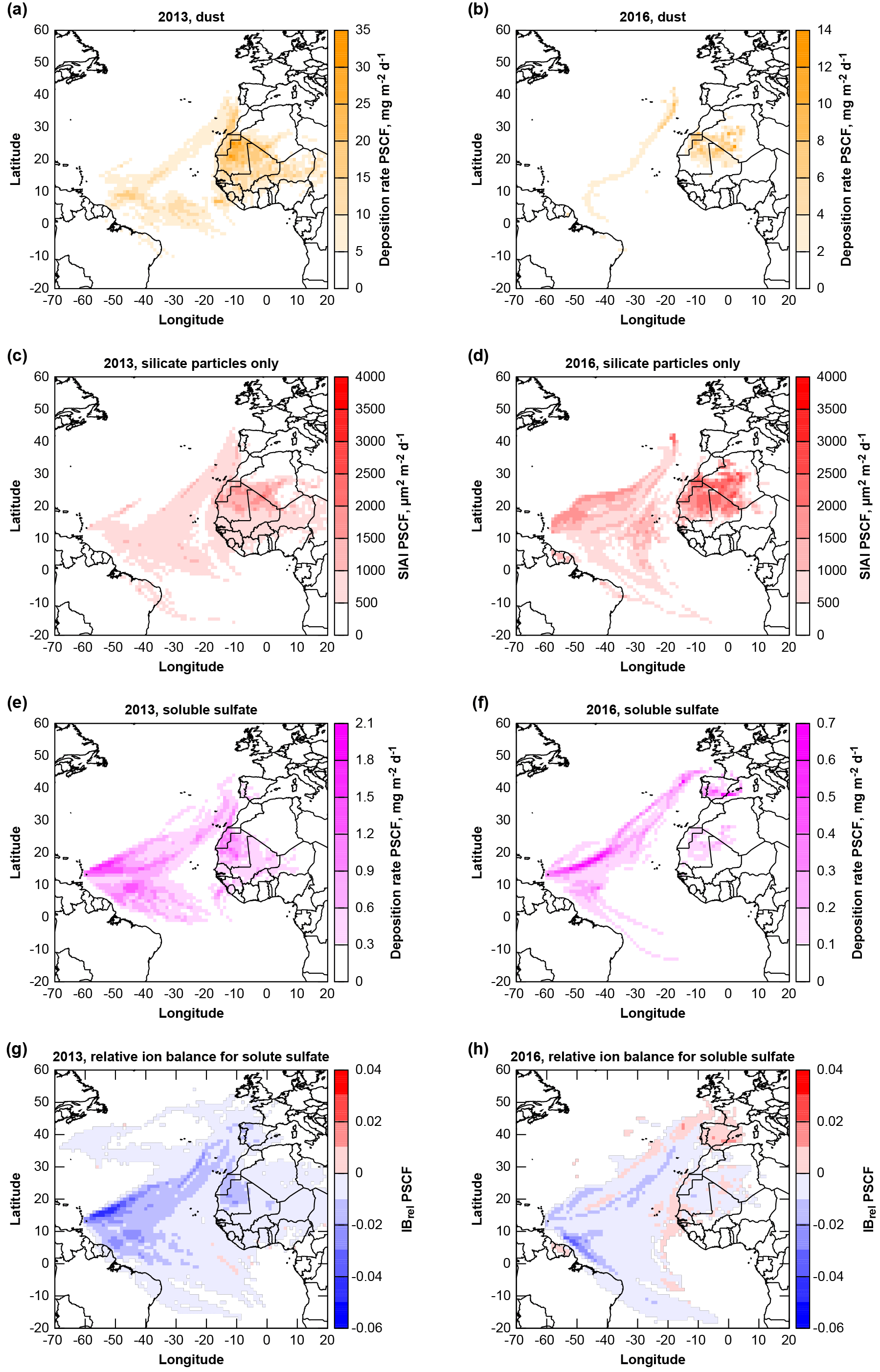
Figure 14 Potential source contribution functions (PSCF) of deposited material: dust (a, b), geometric silicate iron availability index SIAI (c, d), total soluble sulfate (e, f) and relative ion balance for sulfate particles (g, h) for 2013 and 2016 at Ragged Point. Note that for panels (a–d), potential provenance is calculated for Saharan Air Layer transport only (i.e., trajectory arrival altitudes >1500 m).

Figure 15 Ca ∕ Na atomic ratio as function of particle dry diameter for all sea salt particles collected at Ragged Point in 2013. Different samplers are shown by color: CI is blue, DPDS is red and FWI is brown.

3.3.2 Air mass history and potential aerosol sources

The air mass provenance of the sampling periods in 2013 and 2016 is generally similar. The trajectories mostly followed the trade-wind path from northwestern Africa and the eastern Atlantic Ocean to Barbados (Fig. S8 in the Supplement). In 2013, the air was coming more frequently from western Africa than in 2016. After Tropical Storm Chantal in 2013, the air mass origin shifted slightly to more southern regions. In a few cases in 2013, air from the northwestern Atlantic Ocean was recirculated into the trade-wind path.

The sea salt deposition rates are not linked to air mass provenance (not shown). The dust provenance for both years (Fig. 14a, b) is, as expected, pointing to West Africa. This source region is also identified by isotope measurements in July–August 2013 (Bozlaker et al., 2018). The soluble sulfate deposition (Fig. 14e, f) is generally linked to three regions, the Atlantic Ocean, West Africa and southwestern Europe. In 2016 in particular, the sulfate sources appear to be located more in Europe and less in Africa. The relative ion balance (Fig. 14g, h) shows mostly slight negative values indicating presence of ${\mathrm{NH}}_{\mathrm{4}}^{+}$ or H⁺. Interestingly, a positive ion excess is observed for European sulfate in 2016, indicating possible presence of ${\mathrm{NO}}_{\mathrm{3}}^{-}$. These observations support the hypothesis that nitrate as well as sulfate associated with dust sources are likely to be from Europe (e.g., anthropogenic origin; Li-Jones and Prospero, 1998).

Iron contribution from dust is of particular interest for marine ecosystems. Therefore, Fig. 14c and d show the silicate SIAI as a proxy for quick iron availability. It is obvious, that the iron-containing silicate particle source is located in West Africa. Northern and southern West Africa as source regions can not be distinguished after transatlantic transport, in contrast to investigations close to the source (Kandler et al., 2007). This is consistent with observations based on isotope analysis, where a homogeneous composition has also been observed on Barbados (Bozlaker et al., 2018). A slightly higher SIAI can be observed in 2016 than in 2013, while the dust deposition rates, in contrast, are lower. While the total iron deposition correlates well with dust deposition (not shown), similar to observations by Trapp et al. (2010), for the SIAI an inverse relationship is found on Barbados, with higher dust deposition rates leading to lower ratios of SIAI to total dust. This correlates to previous findings, where iron solubility decreased with increasing dust concentration (Shi et al., 2011b; Sholkovitz et al., 2012), though no direct causal relationship can be derived (Shi et al., 2011a).

3.3.3 Sea salt composition

When considering sea salt composition, it is generally assumed that except from the sulfate content, aerosol produced from seawater has a major composition, resembling the bulk seawater (Lewis and Schwartz, 2004). However, it was recently shown in the Arctic that a fractionation can also occur with respect to the major composition (Salter et al., 2016). On Barbados, an increasing positive deviation from the nominal value of 0.022 with decreasing particle size is observed for the Ca ∕ Na atomic ratio of sea salt particles (Fig. 15). This indicates that the same effects found by Salter et al. (2016) are present in Caribbean sea salt production. According to the authors, these might be linked to an enrichment of Ca in sea surface micro-layers, but details are not yet known.

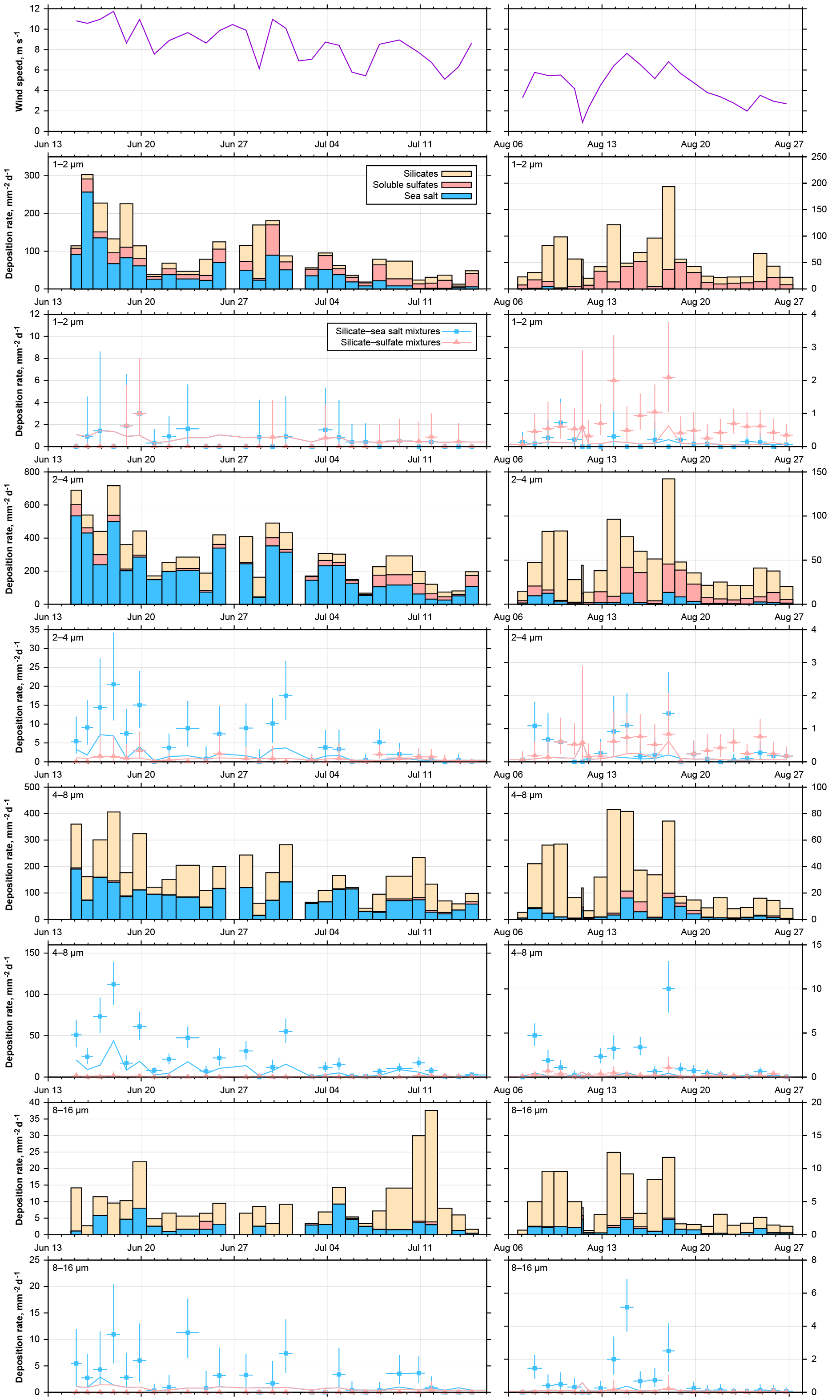
Figure 16 Time series of wind and particle number deposition rates for pure compounds and internally mixed particles for June–July 2013 and August 2016. Particle size ranges are given in the top left of each graph. The limit of detection for the number of internally mixed particles is shown as line in the according color. Where only the detection limit for silicate–sulfate mixtures is visible, both limits are identical.

3.3.4 Abundance of mixed particles

If we consider the abundance of mixed particles on Barbados, a complex picture emerges as function of particle size, time period and available mixing partners (Fig. 16). It can be observed that the total deposition rate for all particle types is linked to the wind speed, which is to be expected from the physical process (see for example Fig. S9 in the Supplement). The higher sea salt deposition rates and also higher concentrations in 2013 in comparison to 2016 are also linked to the wind speed, showing the local sea salt production. In contrast, the dust concentration is slightly lower for higher wind speeds (Fig. S9) for both years. With increasing particle size, the relative abundance of internal dust–sea salt mixtures increases (Fig. 16), but these mixtures only occur when considerable amounts of sea salt are present. This is different for the internal mixture with sulfate. While there are similar ratios of dust and sulfate particles observed in the second half of the 2013 data as in 2016, in 2013, dust–sulfate mixtures are practically absent. Assuming that higher wind speeds in 2013 should lead to more internal mixing, due to increased turbulence, this is clearly indicating that, in contrast to the sea salt–dust mixture, the sulfate–dust mixture has a non-local origin (e.g., Usher et al., 2002).

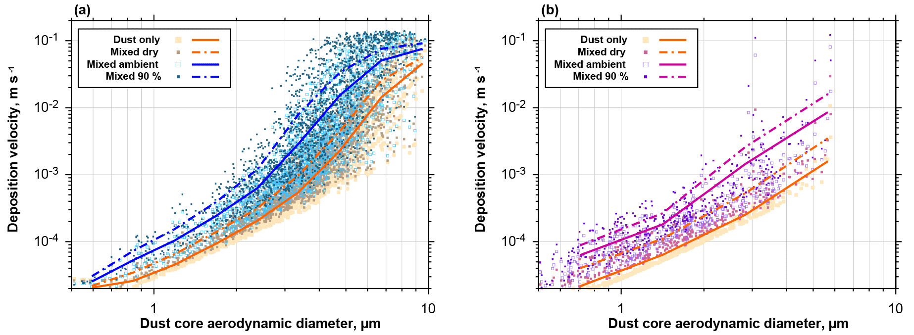
Figure 17 Deposition velocities calculated with the Piskunov model for internal admixture of sea salt (a) or sulfate (b) for the mixed particles observed at Ragged Point. Velocities are given for the unmixed dust core and internal mixtures at dry conditions, at ambient relative humidity and at 90 % relative humidity. The lines show the according means. Note that variation in deposition velocity for the same dust core size arises from variation in wind speed and admixed fraction.

This is corroborated by the dependence of the internal mixtures relative abundance on the single mixing probability (Fig. S11 in the Supplement). If one considers the binary number fraction of mixed particles, i.e., ratio of binary mixed particles to pure compounds, as function of the size-restricted single mixing probability, there is a weak positive correlation with dust–sea salt mixtures for particles larger than 2 µm in diameter, but no correlation with dust–sulfate mixtures. Moreover, for similar single mixing probabilities, the binary number fraction of mixed particles appears slightly higher for higher deposition rates. As the collision efficiency depends on the square of the number concentration (Sundaram and Collins, 1997), this supports the hypothesis of a locally produced internal mixture of sea salt and dust and a non-local production of sulfate and dust, the latter most probably having cloud processing involved (Andreae et al., 1986; Niimura et al., 1998).

The overall ratio of dust–sea salt internal mixture abundance to all dust and sea salt particles increases from 0.01–0.03 for 1 µm particles to 0.1–0.7 for particles of 8–16 µm in diameter, whereas for dust–sulfate mixtures the ratio of 0.01–0.02 is not dependent on particle size. Denjean et al. (2015) report mixed particle abundances of 0.16–0.3, but do not state a size range, so the data can not be compared directly.

If the findings on Barbados are compared to measurements in the eastern Atlantic Ocean (Kandler et al., 2011a), a generally lower abundance of internally mixed particles with respect to dust–sulfate is observed, while comparable abundances of sea salt–dust mixtures are found. While the latter can be explained by similar wind conditions and comparable single mixing probabilities, the former seems to be caused by different aging conditions. Dust arriving over Barbados is transported mostly in the dry Saharan Air Layer (e.g., Schütz, 1980), while dust arriving during winter-time at Cape Verde is transported inside the humid marine boundary layer (Chiapello et al., 1995; Kandler et al., 2011b). Therefore, considerably higher chemical processing rates at Cape Verde due to the higher humidity can be expected (Dlugi et al., 1981; Ullerstam et al., 2002), even though the transport time is most likely shorter. In addition, the boundary layer most probably provides higher concentrations of sulfur compounds for reaction (Davison et al., 1996; Andreae et al., 2000).

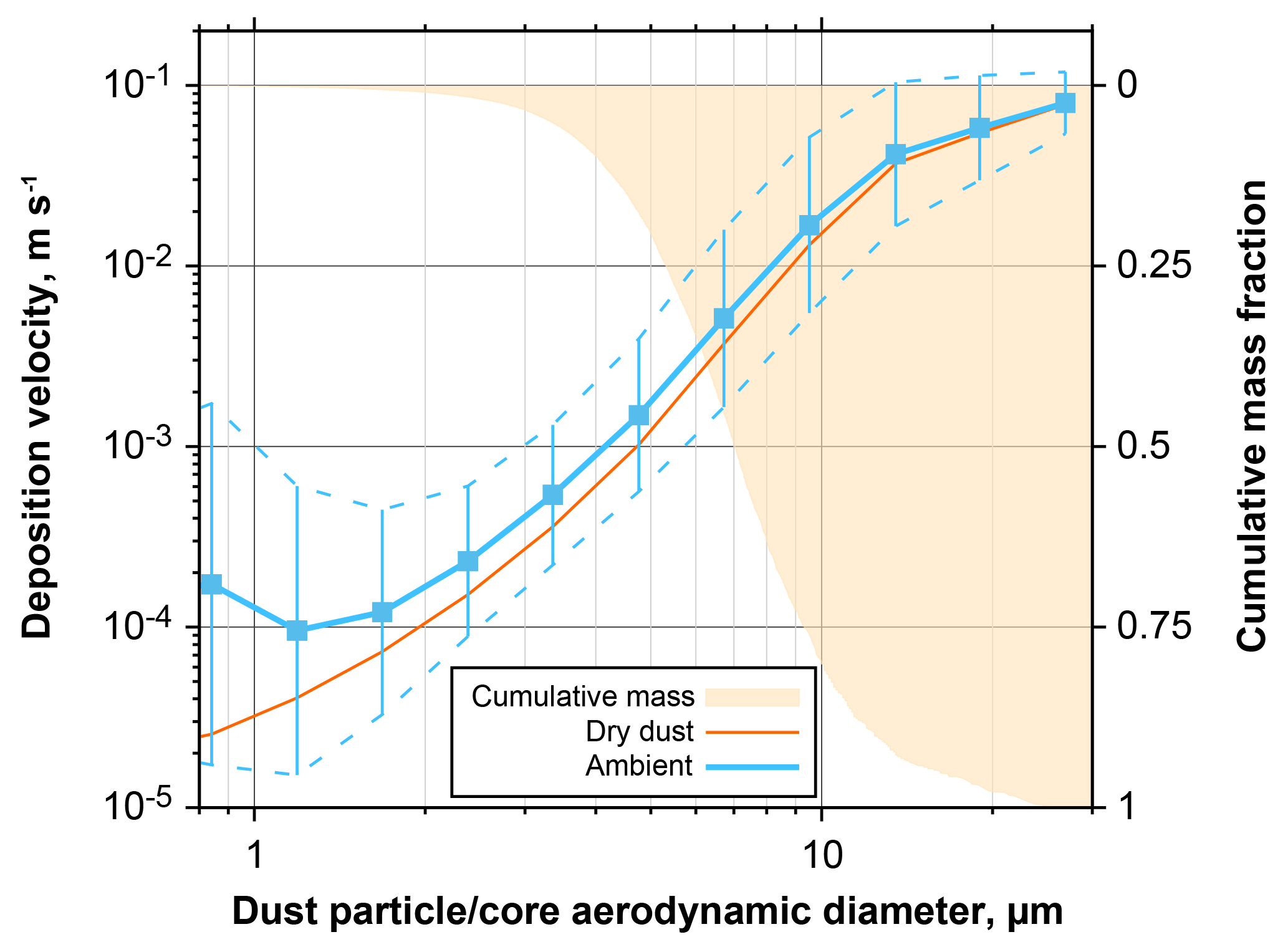
Figure 18 Effective deposition velocity for all dust-containing particles observed at Ragged Point. The blue curves take into account internal mixing and hygroscopic growth at ambient conditions, whereas the orange only regards the dry dust fraction of the particles. In addition, cumulative mass distribution is shown on the inverted right axis. Particle size is given as aerodynamic diameter for the dust fraction of a particle. For the ambient deposition velocity, the geometric mean for each size class is shown in conjunction with the 1 geometric standard deviation range.

Change in dust behavior due to internal particle mixing

If dust particles become internally mixed, their mass, size and hygroscopic behavior change. Therefore, they will have modified deposition velocities as well as hygroscopic properties. Figure 17 shows the increases in deposition velocities for mixed particles observed at Ragged Point in 2013 and 2016. For the both mixtures (dust–sea salt and dust–sulfate), an increase at ambient conditions of a factor of 2–3 is observed for submicron dust particles, which rises to a factor of 5–10 for particles of 3 µm in dust core diameter. As a result, the dust average deposition velocity for particles between 1 and 10 µm in aerodynamic diameter is increased by 30 %–140 % at ambient conditions (Fig. 18). Considering a mass mean aerodynamic diameter in deposition of 7.0 µm, at ambient conditions dust deposition velocity is 6.4 mm s⁻¹, which is an enhancement by approximately 35 % over the unmixed state. This overall value is in the range estimated by Prospero and Arimoto (2009). The enhancement will become more pronounced at higher humidities. It has to be emphasized that this estimate is a lower limit, as there most likely exists mixed particles with a smaller contribution of hygroscopic material, which remain undetected by our analytical approach. At higher humidities, this smaller contribution nevertheless will increase the deposition velocity of the mixtures. While we observe similar relative abundances of mixed particles to previous work in Asian dust outflow (Zhang, 2008), our estimate of impact on deposition is considerably higher. This is mainly related to the use of the Piskunov model, which takes into account turbulent deposition over a Stokes settling approach.

4 Summary and conclusions

Aerosol deposition measurements by means of passive samplers were carried out on a daily basis at Ragged Point, Barbados in June–July 2013 and August 2016. In addition, active aerosol collection was performed with a cascade and a novel free-wing impactor. Size, shape and composition of about 110 000 particles were determined by electron microscopy. Focus was placed in this work on measurement accuracy of chemical composition and mixing state determination for individual particles.

Ragged Point is a high-wind and high-humidity environment (in 2013 in particular), which considerably influences representativeness and accuracy of the different sampling techniques. A deposition model including chemistry-dependent hygroscopic growth was adapted to the sampling situation to assess atmospheric concentration of large particles. Fair agreement was reached between passive and active techniques regarding mass concentration, but clear discrepancies were observed for particle size distribution.

Special attention was paid to the mixing state of dust particles. A model was developed to assess the mixing state of airborne particles by correcting for sampling artifacts due to particle overload, leading to coincidental internal mixing of particles on the substrate (i.e., not representative for the airborne state). Different approaches were tested based on model size distributions and observed particle deposition images. It was found that the size distribution is only weakly affected for substrate area coverages with particles below 10 %. However, the chemical composition of mixtures is already affected at much lower area coverages of <1 %.

During our measurement campaigns, the aerosol was dominated by dust, sea salt and sulfate in changing proportions. The sea salt concentration at Ragged Point is mainly dependent on wind speed. Back trajectory analysis showed that dust is originating from the usual sources in West Africa, and the dust composition with respect to different silicate phases was not varying. Sulfate showed three major potential source areas, Africa, Europe and the Atlantic Ocean. In 2013 in particular, sulfate was more linked to the African source, while in 2016 southwestern Europe occurred as a potential source, with a possible contribution of nitrate.

It was further found that internal mixing of dust and sea salt depends on local wind speed, and we thus hypothesize that it is produced locally, most likely by turbulent processes. In contrast, mixtures of dust and soluble sulfates are presumably not produced locally, but may have formed during the intercontinental transport. Even though the overall amount of internally mixed particles is comparatively low, a considerable impact on total dust deposition velocity is estimated. In addition, a pathway is hypothesized by which the ice-nucleation efficiency of dust can be increased by mixing with soluble compounds during or after the long-range transport.

For future work, the following conclusions can be drawn from our observations.

• If different techniques for deposition and/or atmospheric concentration measurements are compared, it is crucial to measure particle size distributions. We observed in some cases that total mass concentration can compare rather well, even though size distributions, and thus collection efficiencies, are considerably different.

• A better understanding, in theory as well as in experimental use, of particle deposition and collection efficiencies is required in particular under high wind-situations, where turbulent transport has a considerable impact. This most probably applies to a wide range of deposition samplers, not limited to those used in this work.

• When mixing state investigations are done based on collected aerosol particles, the impact of coincidental mixtures on the substrate must be assessed, unless the area coverage with particles is very low (≪1 %). This is particularly the case for larger particles (>5 µm diameter) and for aerosols in the same size range, where similar abundances of different mixing partners exist.

• Internal particle mixing most likely has a considerable influence on dust deposition speed. Future models regarding dust dry deposition should take a deposition speed enhancement by internal mixing into account. The internal mixing also likely increases its efficiency to be activated into cloud droplets (Kelly et al., 2007; Kumar et al., 2011). As a result internally mixed dust particles may be subject to preferential removal by wet deposition. However, more systematic investigations are needed to better understand the mixing processes.

• The intensity of chemical processing might also be affected by the internal mixing, when the particles are activated more efficiently into cloud droplets. For example, the iron solubility for these particles might increase (Shi et al., 2009).

• With respect to a potential cloud impact, the observed fraction of dust mixed with soluble species can be used as input parameters for cloud condensation nuclei parameterizations. Regarding the impact of mixing on dust ice nucleation activity, on one hand studies show a deactivation of dust for high solute concentrations (Zobrist et al., 2008; Iwata and Matsuki, 2018). On the other hand, the more efficient activation into cloud droplets might increase the overall availability of dust for immersion freezing. Further studies are needed to assess and constrain the effects of atmospheric mixing state on ice nucleation in clouds.