Inverse modelling of CF₄ and NF₃ emissions in East Asia

Decadal trends in the atmospheric abundances of carbon tetrafluoride (CF₄) and nitrogen trifluoride (NF₃) have been well characterised and have provided a time series of global total emissions. Information on locations of emissions contributing to the global total, however, is currently poor. We use a unique set of measurements between 2008 and 2015 from the Gosan station, Jeju Island, South Korea (part of the Advanced Global Atmospheric Gases Experiment network), together with an atmospheric transport model, to make spatially disaggregated emission estimates of these gases in East Asia. Due to the poor availability of good prior information for this study, our emission estimates are largely influenced by the atmospheric measurements. Notably, we are able to highlight emission hotspots of NF₃ and CF₄ in South Korea due to the measurement location. We calculate emissions of CF₄ to be quite constant between the years 2008 and 2015 for both China and South Korea, with 2015 emissions calculated at 4.3±2.7 and 0.36±0.11 Gg yr⁻¹, respectively. Emission estimates of NF₃ from South Korea could be made with relatively small uncertainty at 0.6±0.07 Gg yr⁻¹ in 2015, which equates to ∼1.6 % of the country's CO₂ emissions. We also apply our method to calculate emissions of CHF₃ (HFC-23) between 2008 and 2012, for which our results find good agreement with other studies and which helps support our choice in methodology for CF₄ and NF₃.

1 Introduction

The major greenhouse gases (GHGs) – carbon dioxide, methane, and nitrous oxide – have natural and anthropogenic sources. The synthetic fluorinated species – chlorofluorocarbons (CFCs), hydrochlorofluorocarbons (HCFCs), hydrofluorocarbons (HFCs), and perfluorocarbons (PFCs), sulfur hexafluoride (SF₆) and nitrogen trifluoride (NF₃) – are almost or entirely anthropogenic and are released from industrial and domestic appliances and applications. Of the synthetic species, tetrafluoromethane (CF₄) and NF₃ are emitted nearly exclusively from point sources of specialised industries (Arnold et al., 2013; Mühle et al., 2010, Worton et al., 2007). Although these species currently make up only a small percentage of current emissions contributing to global radiative forcing, they have potential to form large portions of specific company, sector, state, province, or even country level GHG budgets.

CF₄ is the longest-lived GHG known, with an estimated lifetime of 50 000 years, leading to a global warming potential on a 100-year timescale (GWP₁₀₀) of 6630 (Myhre et al., 2013). Significant increases in atmospheric concentrations are ascribed mainly to emissions from primary aluminum production during so-called “anode events” when the alumina feed to the reduction cell is restricted (International Aluminium Institute, 2016), and from the microchip-manufacturing component of the semiconductor industry (Illuzzi and Thewissen, 2010). Recently, evidence emerged that, similar to primary aluminium production, rare earth element production may also release substantial amounts of CF₄ (Vogel et al., 2017; Zhang et al., 2017). Other emission sources for CF₄ include release during the production of SF₆ and HCFC-22, but emissions from these sources are estimated to be small compared to the emissions from the aluminium production and semiconductor manufacturing industries (EC-JRC/PBL, 2013; Mühle et al., 2010). There is also a very small natural emission source of CF₄, sufficient to maintain the pre-industrial atmospheric burden (Deeds et al., 2008; Worton et al., 2007).

According to the Intergovernmental Panel on Climate Change (IPCC) fifth assessment, NF₃'s global warming potential on a 100-year timescale (GWP₁₀₀) is ∼16 100 (based on an atmospheric lifetime of 500 years) (Myhre et al., 2013); however, recent work suggests the GWP₁₀₀ is higher at 19 700 due to an increased estimate in the radiative efficiency (Totterdill et al., 2016). Use of NF₃ began in the 1960s in specialty applications, e.g. as a rocket fuel oxidiser and as a fluorine donor for chemical lasers (Bronfin and Hazlett, 1966). Beginning in the late 1990s, NF₃ has been used by the semiconductor industry, and in the production of photovoltaic cells and flat-panel displays. NF₃ can be broken down into reactive fluorine (F) radicals and ions, which are used to remove the remaining silicon-containing deposits in process chambers (Henderson and Woytek, 1994; Johnson et al., 2000). NF₃ was also chosen because of its promise as an environmentally friendly alternative, with conversion efficiencies to create reactive F far higher than other compounds such as C₂F₆ (Johnson et al., 2000; International SEMATECH Manufacturing Initiative, 2005). Given its rapid recent rise in the global atmosphere and projected future market, it has been estimated that NF₃ could become the fastest growing contributor to radiative forcing of all the synthetic GHGs by 2050 (Rigby et al., 2014).

CF₄ and NF₃ are not the only species with major point source emissions. Trifluoromethane (CHF₃; HFC-23) is principally made as a byproduct in the production of chlorodifluoromethane (CHClF₂, HCFC-22). Of the HFCs, HFC-23 has the highest 100-year global warming potential (GWP₁₀₀) at 12 400, most significantly due to a long atmospheric lifetime of 222 years (Myhre et al., 2013). Its regional and global emissions have been the subject of numerous previous studies (Fang et al., 2014, 2015; McCulloch and Lindley, 2007; Miller et al., 2010; Montzka et al., 2010; Stohl et al., 2010; Li et al., 2011; Kim et al., 2010; Yao et al., 2012; Keller et al., 2012; Yokouchi et al., 2006; Simmonds et al., 2018). Thus, emissions of HFC-23 are already relatively well characterised from a bottom-up and a top-down perspective. In this work, we will also calculate HFC-23 emissions, not to add to current knowledge, but to provide a level of confidence for our methodology.

Unlike for HFC-23, the spatial distribution of emissions responsible for CF₄ and NF₃ abundances is very poorly understood, which is hindering action for targeting mitigation. HFC-23 is emitted from well-known sources (namely HCFC-22 production sites) with well-characterised estimates of emission magnitudes, and hence it has been a target for successful mitigation (by thermal destruction) via the clean development mechanism (Miller et al., 2010). However, emissions of CF₄ and NF₃ are very difficult to estimate from industry level information: emissions from Al production are highly variable depending on the conditions of manufacturing, and emissions from the electronics industry depend on what is being manufactured, the company's recipes for production (such information is not publicly available), and whether abatement methods are used and how efficient these are under real conditions. Both the Al production and semiconductor industries have launched voluntary efforts to control their emissions of these substances, reporting success in meeting their goals (International Aluminium Institute, 2016; Illuzzi and Thewissen, 2010; World Semiconductor Council, 2017). Despite the industry's efforts to reduce emissions, top-down studies on the emissions of CF₄ and NF₃ have shown the bottom-up inventories are likely to be highly inaccurate. Most recently, Kim et al. (2014) showed that global bottom-up estimates for CF₄ are as much as 50 % lower than top-down estimates, and Arnold et al. (2013) showed that the best estimates of global NF₃ emissions calculated from industry information and statistical data total only ∼35 % of those estimated from atmospheric measurements.

Accurate emission estimates of NF₃ and CF₄ are difficult to make based on simple parameters such as integrated country level uptake rates and leakage rates, which, for example, underpin calculations of HFC emissions. Active or passive activities to reduce emissions vary between countries, and between industries and companies within countries, and the impetus to accurately understand emissions is lacking in regions that have not been required to report emissions under the United Nations Framework Convention on Climate Change (UNFCCC). This problem is compounded by the difficulty in making measurements of these gases: CF₄ and NF₃ are the two most volatile GHGs after methane, and have very low atmospheric abundances, which makes routine measurements in the field at the required precision particularly difficult. The Advanced Global Atmospheric Gases Experiment (AGAGE) has been monitoring the global atmospheric trace gas budget for decades (Prinn et al., 2018). Most recently, AGAGE's “Medusa” preconcentration GC-MS (gas chromatography–mass spectrometry) system has been able to measure a full suite of the long-lived halogenated GHGs (Arnold et al., 2012; Miller et al., 2008). The Medusa is the only instrument demonstrated to measure NF₃ in ambient air samples and the only field-deployable instrument capable of measuring CF₄. The Medusa on Jeju Island, South Korea, is one of only 20 such instruments currently in operation globally and is uniquely sensitive to the dominant emission sources of these compounds given its location in this highly industrial part of the globe with large capacities of Al production, semiconductor manufacturing, and rare Earth element production industries. Its utility has already been demonstrated in numerous previous studies to understand emissions of many GHGs from Japan, South Korea, North Korea, eastern China, and surrounding countries (Fang et al., 2015; Kim et al., 2010; Li et al., 2011).

For the first time, we use the measurements of CF₄ (starting in 2008) and NF₃ (starting in 2013) in an inversion framework – coupling each measurement with an air history map computed using a particle dispersion model. We demonstrate the use of these measurements to find emission hotspots in this unique region with minimal use of prior information, and we show that East Asia is a major source of these species. Focussed mitigation efforts, based on these results, could have a significant impact on reducing GHG emissions from specific areas. The technology for abating emissions of these gases from such discrete sources exists and could be used (Chang and Chang, 2006; Purohit and Höglund-Isaksson, 2017; Illuzzi and Thewissen, 2010; Yang et al., 2009; Raoux, 2007; Wangxing et al., 2016).

2 Methods

2.1 Atmospheric measurements

The Gosan station (from here on termed GSN) is located on the south-western tip of Jeju Island in South Korea (33.29244^∘ N, 126.16181^∘ E). The station rests at the top of a 72 m cliff, about 100 km south of the Korean Peninsula, 500 km north-east of Shanghai, China, and 250 km west of Kyushu, Japan, with an air inlet 17 m above ground level (a.g.l.).

A Medusa GC-MS system was installed at GSN in 2007 and has been operated as part of the AGAGE network to take automated, high-precision measurements for a wide range of CFCs, HCFCs, HFCs, PFCs, Halons, and other halocarbons, and all significant synthetic GHGs and/or stratospheric ozone-depleting gases as well as many naturally occurring halogenated compounds (Miller et al., 2008; Arnold et al., 2012; Kim et al., 2010). Since November 2013, NF₃ has been measured within this suite of gases. Air reaches GSN from the most heavily developed areas of East Asia, making the measurements and their interpretation a unique source for top-down emission estimates in the region. Ambient air measurements are made every 130 min and are bracketed with a standard before and after the air sample in order to correct for instrumental drift in calibration. Further details on the methodology for the calibration of these gases are given elsewhere (Arnold et al., 2012; Mühle et al., 2010; Miller et al., 2010; Prinn et al., 2018).

2.2 Atmospheric model

Lagrangian particle dispersion models are well suited to determine emissions of trace gases on this spatial scale as they can be run backwards, allowing for the source–receptor relationship to be efficiently calculated. We use the Numerical Atmospheric dispersion Modelling Environment (NAME III), henceforth called NAME, developed by the UK Met Office (Ryall and Maryon, 1998; Jones et al., 2007). Inert particles are advected backwards in time by the transport model, NAME, which also associates a mass to each trajectory. Hence, NAME output is provided as the time-integrated near-surface (0–40 m) air concentration (g s m⁻³) in each grid cell – the surface influence resulting from a conceptual release at a specific rate (g s⁻¹) from the site. “Offline”, this surface influence is divided by the total mass emitted during the 1 h release time and multiplied by the geographical area of each grid box to form a new array with each component representative of how 1 g m⁻² s⁻¹ of continuous emissions from a grid square would result in a measured concentration at the model's release point (the measurement site). Multiplication of each grid component by an emission rate then results in a contribution to the concentration.

The meteorological parameter inputs to NAME are from the Met Office's operational global NWP model, the Unified Model (UM) (Cullen, 1993). The UM had a horizontal resolution of $\mathrm{0.5625}{}^{\circ }\times \mathrm{0.375}{}^{\circ }$ (∼40 km) from December 2007 to April 2010; $\mathrm{0.3516}{}^{\circ }\times \mathrm{0.2344}{}^{\circ }$ (∼25 km) from April 2010 to July 2014; and $\mathrm{0.234375}\times \mathrm{0.15625}{}^{\circ }$ (∼17 km) from mid-July 2014 to mid-July 2017. The number of vertical levels in the UM has increased over this period, with NAME taking the lowest 31 levels in 2009 and the lowest 59 levels in 2015. The GHGs considered in this study have lifetimes on the order of hundreds to tens of thousands of years (Myhre et al., 2013) and can be considered inert gases on the spatial and temporal scales of this study, and therefore the NAME model schemes for representing chemistry, dry deposition, wet deposition, and radioactive decay were not used. The planetary boundary layer height (BLH) estimates are taken from the UM; however, a minimum BLH allowed within NAME was set to 40 m to be consistent with the maximum emission height and the height of the output grid. The NAME model was run to estimate the 30-day history of the air on the route to GSN. We calculated the time-integrated air concentration (dosage) at each grid box ($\mathrm{0.352}{}^{\circ }\times \mathrm{0.234}{}^{\circ }$, 0–40 m a.g.l., irrespective of the underlying UM meteorology resolution) from a release of 1 g s⁻¹ at GSN at 17±10 m a.g.l.

The model is three-dimensional, and therefore it is not just surface-to-surface transport that is modelled: an air parcel can travel from the surface to a high altitude and then back to the surface, but only those times when the air parcel is within the lowest 40 m above the ground will be included in the model output aggregated sensitivity maps. The computational domain covers 54.34^∘ E to 168.028^∘ W longitude (391 grid cells of dimension 0.352^∘) and 5.3^∘ S to 74.26^∘ N latitude (340 grid cells of dimension 0.234^∘), and extends to more than 19 km vertically. Despite the increase in the resolution of the UM over the time period covered, the resolution of the NAME output was kept constant throughout. For each 1 h period, 5000 inert model particles were used to describe the dispersion of air. By dividing the dosage (g s m⁻³) by the total mass emitted (3600 s h⁻¹ × 1 h × 1 g s⁻¹) and multiplying by the geographical area of each grid box (m²), the model output was converted into a dilution matrix H (s m⁻¹). In Fig. 1, we show an aggregated dilution matrix for the 2013 inversion period, demonstrating the areas of most significant influence on the GSN measurements. Each element of the matrix H dilutes a continuous emission of 1 g m⁻² s⁻¹ from a given grid box over the previous 30 days to simulate an average concentration (g m⁻³) at the receptor (measurement point) during a 1 h period.

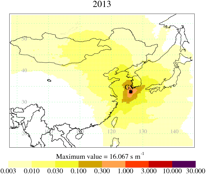
Figure 1 An aggregation of the dilution matrices from 2013, generated using NAME output (see Sect. 2.2), illustrating the relative sensitivity of measurements at GSN to emissions in the region.

2.3 Inversion framework

For most long-lived trace gases (with lifetimes of years or longer), the assumption that atmospheric mole fractions respond linearly to changes in emissions holds well. By using this linearity, we can relate a vector of observations (y) to a state vector (x) made up of emissions and other non-prescribed model conditions (see Sect. 2.6) via a sensitivity matrix (H) (Tarantola, 2005):

$${\displaystyle }\mathit{y}=\mathbf{H}\mathit{x}+\mathrm{residual}.$$

A Bayesian framework is typically used in trace gas inversions and incorporates a priori information, which gives rise to the following cost function:

$$\begin{array}{}\text{(1)}& C={\left(\mathbf{H}\mathit{x}-\mathit{y}\right)}^T{\mathbf{R}}^{-\mathrm{1}}\left(\mathbf{H}\mathit{x}-\mathit{y}\right)+(\mathit{x}-{\mathit{x}}_{\mathrm{p}}{)}^T{\mathbf{B}}^{-\mathrm{1}}(\mathit{x}-{\mathit{x}}_{\mathrm{p}}),\end{array}$$

where C is the cost function score (the aim is to minimise this score); H is made up mainly of the model-derived dilution matrices (Sect. 2.2) but also the sensitivity of changes in domain border conditions on measured mixing ratios; x is a vector of emissions and domain border conditions; y is a vector of observations; R is a matrix of combined model and observation uncertainties; x_p is a vector of prior estimates of emissions and domain border conditions; and B is an error matrix associated with x_p. The cost function is minimised using a non-negative least squares fit (NNLS) (Lawson and Hanson, 1974), as previously used for volcanic ash (Thomson et al., 2017; Webster et al., 2017). The NNLS algorithm finds the least squares fit under the constraint that the emissions are non-negative. This is an “active set” method which efficiently iterates over choices for the set of emissions for which the non-negative constraint is active, i.e. the set of emissions which are set to zero.

The first term in Eq. (1) describes the mismatch (fit) between the modelled time series and the observed time series at each observation station. The observed concentrations (y) are comprised of two distinct components: (a) the Northern Hemisphere (NH) background concentration, referred to as the baseline, that changes only slowly over time, and (b) rapidly varying perturbations above the baseline. These observed deviations above background (baseline) are assumed to be caused by emissions on a regional scale that have yet to be fully mixed on the hemisphere scale. The magnitude of these deviations from baseline and, crucially, how they change as the air arriving at the stations travels over different areas, is the key to understanding where the emissions have occurred. The inversion system considers all of these changes in the magnitude of the deviations from baseline as it searches for the best match between the observations and the modelled time series. The second term describes the mismatch (fit) between the estimated emissions and domain border conditions (x) and prior estimated emissions and domain border conditions (x_p) considering the associated uncertainties (B).

The aim of the inversion method is to estimate the spatial distribution of emissions across a defined geographical area. The emissions are assumed to be constant in time over the inversion time period (in this case, one calendar year, as is typically reported in inventories). Assuming the emissions are invariant over long periods of time is a simplification but is necessary given the limited number of observations available. In order to compare the measurements and the model time series, the latter are converted from air concentration (g m⁻³) to the measured mole fraction, e.g. parts per trillion (ppt), using the modelled temperature and pressure at the observation point.

2.4 Prior emission information

Global emission estimates of CF₄ and NF₃ using atmospheric measurements have demonstrated that bottom-up accounting methods for one or more sectors, or one or more regions, are highly inaccurate (Arnold et al., 2013; Mühle et al., 2010). This study makes no effort to improve such inventory methods but instead focusses on minimising the reliance of prior information on our Bayesian-based posterior emission estimates. Our prior information data sets come from the Emissions Database for Global Atmospheric Research (EDGAR) v4.2 emission grid maps (EC-JRC/PBL, 2013). This data set only covers the years 2000 to 2010, and therefore we apply the prior for 2010 for each year between 2011 and 2015. The 0.1×0.1^∘ EDGAR emission maps were first regridded based on the lower resolution of our inversion grid ($\mathrm{0.3516}{}^{\circ }\times \mathrm{0.2344}{}^{\circ }$). In order to remove the influence of the within-country prior spatial emission distribution, each country's emissions were then averaged across their entire landmass (see Fig. S1 in the Supplement). We applied five different levels of uncertainty to each inversion grid cell (a,b) in five separate inversion experiments, each a multiple of the emission magnitude (x_a,b) in each grid cell: $\mathrm{1}\times x_{a,b}$ (i.e. 100 % uncertainty), $\mathrm{10}\times x_{a,b}$, $\mathrm{100}\times x_{a,b}$, $\mathrm{1000}\times x_{a,b}$, and $\mathrm{10}\mathrm{000}\times x_{a,b}$. We were then able to test the sensitivity of the prior emission uncertainty and provide evidence for the low influence of prior information on the emission estimates in the posterior.

2.5 Measurement–model and prior uncertainties

In addition to inaccurate prior information, another significant source of uncertainty in estimating emissions is from the model, from both the input meteorology and the atmospheric transport model itself. The uncertainty matrix, R, is a critical part of Eq. (1) that allows us to adjust uncertainties assigned to each measurement depending on how well we think the model is performing at that time. It describes, per hour time period, a combined uncertainty of the model and the observation at each time. The method of assigning measurement–model uncertainties is under development and here we describe one method that has been applied to the modelling of GSN measurements. All elements of the modelled meteorology (wind speed and direction, BLH, temperature, pressure, etc.) are important in understanding the dilution and uncertainty in modelling from source to receptor. However, quantifying the impact of each element that each model particle experiences in order to fully quantify the model uncertainty at each measurement time is beyond what is available from numerical weather prediction models. So in order to attempt to quantify a model/observation uncertainty we took a pragmatic approach and used modelled BLH at the receptor as a proxy.

Emissions are primarily diluted by transport and mixing within the planetary boundary layer (PBL), and hence modelling of the PBL height (BLH) is crucial for accurate modelling of the mixing ratios. Changes in BLH at or surrounding the measurement location can cause significant changes to the measured mixing ratio. A low BLH (causing a larger model uncertainty) has two implications for measurements at the Gosan site. The first implication is a greater possibility of air from above the PBL being sampled in reality but not in the model. Subtle changes in the BLH at the exact measurement location are not well modelled and the difference between sampling above or within the PBL can have a significant influence on the amount of pollutant assigned to a back trajectory. The second implication is greater influence of emissions from sources very near GSN. A lower BLH means that a lower rate of dilution of local emissions will occur, in turn increasing the signal of the local pollutant above the baseline. A relatively small change in a low BLH will have a significant influence on this dilution compared to the same change on a high BLH. Thus, any error in the BLH at low levels can significantly amplify the uncertainty in the pollutant dilution. This is coupled with the fact that the modelled BLH has significant uncertainty especially when low.

To assign a model uncertainty to each hourly window of measurements, we use model information of BLH:

$${\displaystyle }{\mathit{\sigma }}_{\mathrm{model}}={\mathit{\sigma }}_{\mathrm{baseline}}\times f_{\mathrm{BLH}},$$

where σ_baseline is the variability associated with the baseline calculation (see Sect. 2.6), and f_BLH is a multiplying factor (greater than or less than unity) that increases or decreases the relative uncertainty assigned to each model time period. f_BLH is based on modelled BLH magnitude and variability over a 3 h period and is calculated with the following:

$${\displaystyle }{f}_{\mathrm{BLH}}={\displaystyle \frac{{\mathrm{Max}}_{\text{BLH-inlet}}}{{\mathrm{Min}}_{\text{BLH-inlet}}}}\times {\displaystyle \frac{\mathrm{Threshold}}{{\mathrm{Min}}_{\mathrm{BLH}}}},$$

where Max_BLH-inlet is the largest of either 100 m or the maximum distance, calculated hourly, between the inlet and the modelled BLH within a period of 3 h around the measurement time; Min_BLH-inlet is the smallest of the distances calculated between the inlet and the BLH over the same 3 h period; “Threshold” is an arbitrary value set at 500 m; and Min_BLH is the lowest BLH recorded over the 3 h period. Thus, the relative assigned uncertainty considers the proximity of the varying BLH to the inlet height and a recognition that observations taken when the BLH is varying at higher altitudes (> 500 m a.g.l.) is likely to have less impact and therefore have lower uncertainty compared to those taken when the BLH is varying at lower altitudes (< 500 m a.g.l.).

Figures S2–S6 show annual time series of observations and the corresponding measurement–model uncertainties, as well as statistics for the mismatch between observations and modelled time series.

2.6 Baseline calculation and domain border conditions

For each measurement at GSN, it is important to accurately understand the portion of the total mixing ratio arriving from outside the inversion domain and the portion from emission sources within the domain; otherwise, emissions from specific areas could be over- or underestimated. GSN is uniquely situated, receiving air masses from all directions over the course of the year, which can have distinct compositions of trace gases, driven mainly by the different emission rates between the two hemispheres and slow interhemispheric mixing.

In addition to the time-integrated air concentration produced by NAME (Sect. 2.2), the 3-D coordinate where each particle left the computational domain was also recorded. This information was then post-processed to produce the percentage contributions from 11 different borders of the 3-D domain (Fig. 2). From 0 to 6 km in height, eight horizontal boundaries (WSW, WNW, NNW, NNE, ENE, ESE, SSE, and SSW) were considered, and between 6 and 9 km the horizontal boundaries were only split between north and south. The 11th border was considered when particles left in any direction above 9 km. Thus, the influence of air arriving at GSN from outside the domain was simplified as a combination of air masses arriving from 11 discrete directions.

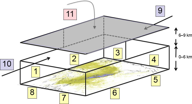
Figure 2 Schematic of the domain borders as applied in the inversion. A total of 11 domain border conditions were estimated as depicted from 1 to 11 as a multiplying factor to the prior baseline estimated using data from the Mace Head observatory. Below 6 km, the domain border was divided eight times: NNE, ENE, ESE, SSE, SSW, WSW, WNW, and NNW; between 6 and 9 km, the domain border was just divided between north and south; and air arriving from above 9 km was considered from one “high” domain border. Average posterior multiplying factors for CF₄ over the 8 years were 1.00±0.01 (NNE), 0.97±0.06 (ENE), 1.02±0.05 (ESE), 0.99±0.01 (SSE), 1.00±0.01 (SSW), 0.99±0.01 (WSW), 1.00±0.00 (WNW), 1.00±0.01 (NNW), 1.00±0.00 (6 to 9 km north), 1.00±0.05 (6 to 9 km south), and 0.97±0.03 (above 9 km).

We use measurements from the Mace Head observatory (from here termed MHD) on the west coast of Ireland (53.33^∘ N, 9.90^∘ W) – a key AGAGE site providing long-term in situ atmospheric measurements – to act as a starting point for an estimate of the composition of air from the NH midlatitudes entering the East Asian domain. MHD was one of the first locations to measure CF₄ (starting 2004) and NF₃ (starting 2012), and other measurements from the site are routinely used in atmospheric studies to calculate decadal trends in the NH atmospheric abundances. In summary, a quadratic fit was made only to MHD observations that were representative of the NH baseline, i.e. when well-mixed air was arriving predominately from the WNW–NNW (North Atlantic) direction as calculated using NAME (details of filtering and fitting are given in the Supplement).

The composition of air arriving from any of the 11 directions is calculated using corresponding multiplying factors applied to the MHD baseline, which were included as part of the state vector (x); i.e. these factors are constant for a given inversion year. The prior baseline was therefore perturbed as part of the inversion based on the relative contribution of air arriving from different borders of the 3-D domain and the multiplying factors that are included within the cost function (Eq. 1). Figure 3 shows an annual time series of observations for CF₄ and the difference between the prior baseline (the quadratic fit from MHD) and the posterior baseline.

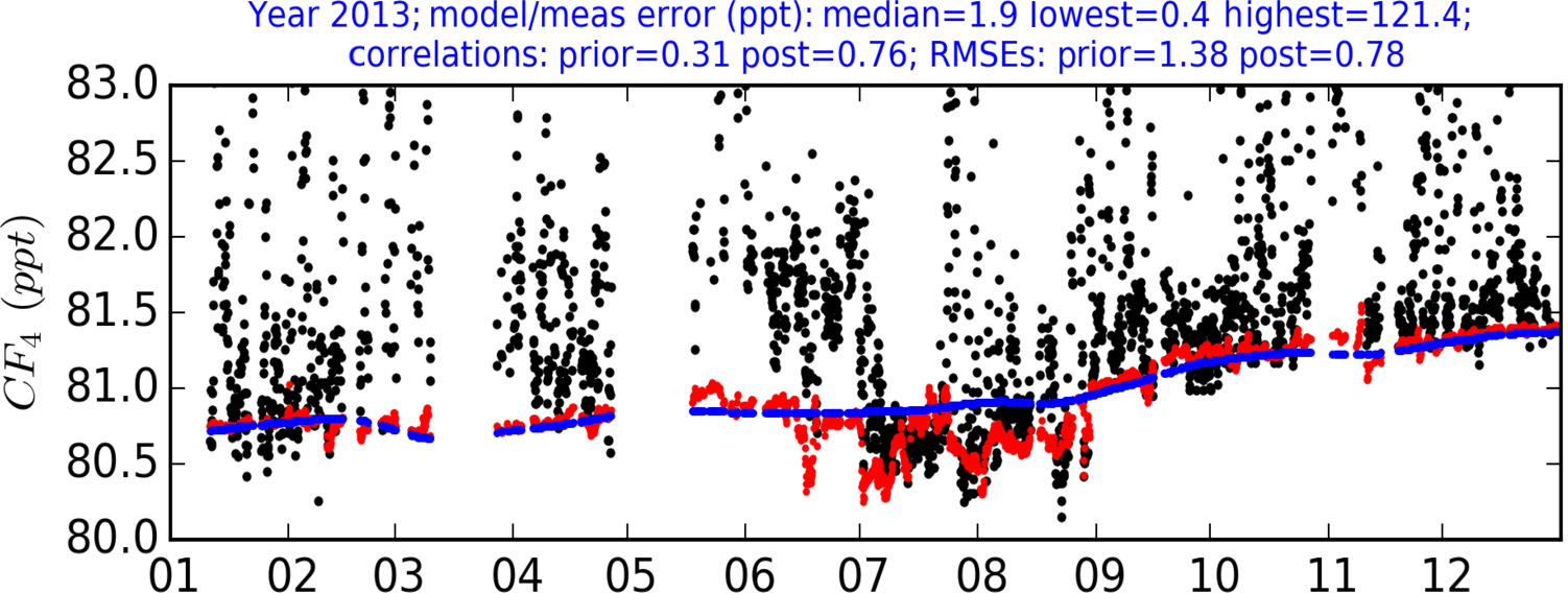
Figure 3 Time series of CF₄ measurements during 2013 – an example year with the most uninterrupted time series. Prior baseline (blue) is adjusted in the inversion using the baseline condition variables, producing a posterior baseline (red). During the summer months, the proportion of air arriving from the south significantly rises, causing a large shift in the posterior baseline relative to the prior baseline calculated from Mace Head data.

2.7 Domains and inversion grids

The domain used in the inversion is smaller than the computational NAME transport model domain. The horizontal inversion domain covers 88.132 to 145.860^∘ E longitude (164 fine grid cells of 0.352^∘) and 15.994 to 57.646^∘ N latitude (178 fine grid cells of 0.234^∘). GSN is within a region surrounded by countries with major developed industries, and therefore the site is relatively insensitive to emissions from further away that are diluted on the route to the site. NAME is run on a larger domain to ensure that on the occasion when air circulates out of the inversion domain and then back, its full 30-day history in the inversion domain is included.

An initial computational inversion grid (from here termed the “coarse grid”) was created based on (a) aggregated information from the NAME footprints over the period of the inversion (in this case, 1 year), aggregating fewer grid cells in areas that are “seen” the most by GSN, and (b) the prior emissions flux; i.e. areas known to have low emissions (e.g. ocean) had higher aggregation. Coarse grid cells could not be aggregated over more than a single country/region and a total of ≈100 coarse grid cells (n) were created. After the initial inversion, a coarse grid cell was chosen to divide in two by area. The decision on which single coarse grid cell to split is calculated based on the posterior emission density (g yr⁻¹ m⁻²) of the coarse grids and the ability of the posterior emissions to impact the measurements at GSN (using information from the NAME output). A new inversion was run using identical inputs except for the number of grid cells (now n+1). This sequence was repeated 50 times, creating ≈150 coarse grid cells within the inversion domain for the final inversion. The results from the inversions with the maximum disaggregation are presented in this paper.

Table 1 Annual posterior emission estimates for the five main emitting countries surrounding GSN (Gg yr⁻¹). These posterior emission estimates are from the inversion that uses a prior emission uncertainty on each fine grid cell of 100 times the prior emission rate.

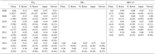
^* Kim et al. (2010) estimated CF₄ emissions from China in the range 1.7–3.1 Gg yr⁻¹ and Li et al. (2011) in the range 1.4–2.9 Gg yr⁻¹. For South and North Korea (combined), Li et al. (2011) estimated emissions of CF₄ at 0.19–0.26 Gg yr⁻¹ and from Japan at 0.2–0.3 Gg yr⁻¹.

3 Results and discussion

3.1 Country total emission estimates

Table 1 provides a summary of our estimates of emissions from the five major emitting countries/regions within the East Asian domain. These posterior emission estimates use a prior emission uncertainty in each fine grid cell of 100 times the emission magnitude (see Sect. 2.4).

HFC-23

Figure 4 Time series of country emission totals (2008–2015). Annual inversion results are given for each gas for three different levels of uncertainty applied to the prior emission map: 100, 1000, and 10 000 times the emission magnitude for each grid cell. The aggregated country totals from the prior data set are also given. Posterior uncertainties are shown for the 100 times prior uncertainty scenario.

Fang et al. (2015) conducted a very thorough bottom-up study within their work on HFC-23, constraining an inversion model using both prior information and atmospheric measurements. They used an inverse method based on the FLEXible PARTicle dispersion model (FLEXPART) using measurements from three sites in East Asia – GSN, Hateruma (a Japanese island ∼200 km east of Taiwan), and Cape Ochiishi (northern Japan), calculating an HFC-23 emission rise in China from 6.4±0.7 Gg yr⁻¹ in 2007 (6.2±0.6 Gg yr⁻¹ in 2008) to 8.8±0.8 Gg yr⁻¹ in 2012. An earlier study by Stohl et al. (2010) also reports HFC-23 emissions of 6.2±0.8 Gg yr⁻¹ in 2008. Both Fang et al. (2015) and Stohl et al. (2010) report emissions from other countries below 0.25 Gg yr⁻¹ for all years. Our estimates use a completely independent inverse method and only data from GSN, yet the results are very close to those of Fang et al. (2015) (Fig. 4) – 6.8±4.3 Gg yr⁻¹ in 2008 (a difference of 10 %) and 10.7±4.6 Gg yr⁻¹ in 2012 (a difference of 22 %) – and of Stohl et al. (2010). The posterior uncertainties in these two different studies mainly reflect the difference in the prior uncertainty assumed for the prior information. We assume a very high level of uncertainty on our prior emissions, and therefore our posterior uncertainties are significantly higher. However, these inversion result estimates are lower than estimates based on interspecies correlation analysis by Li et al. (2011) who calculated emissions of HFC-23 from China in 2008 in the range of 7.2–13 Gg yr⁻¹. Using a CO tracer-ratio method, Yao et al. (2012) estimated particularly low emissions of 2.1±4.6 Gg yr⁻¹ for 2011–2012. The estimates derived from atmospheric inversions do not rely on any correlations with other species or known emissions for certain species and, given two separate inversion studies, have produced very similar results. We suggest these provide a more reliable top-down emission estimate of HFC-23. As well as providing an independent validation of the previous work on HFC-23 by Fang et al. (2015) and Stohl et al. (2010), the alignment of our HFC-23 emission estimates with those previous studies provides confidence in our inversion methodology for the CF₄ and NF₃ emission estimates.

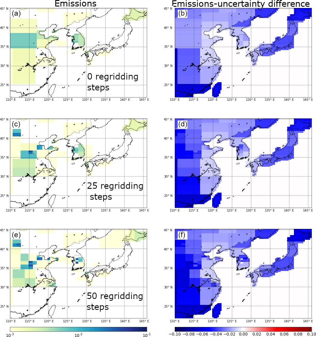
Figure 5 The effect of the regridding routine on posterior emission distributions for CF₄. Panels (a), (c), and (e) are posterior emission maps at the initial inversion resolution, at 0 regridding steps, at 25 regridding steps, and at 50 regridding steps, respectively. Panels (b), (d), and (f) show the emission magnitude minus the uncertainty calculated for each inversion grid box at the same regridding levels (0, 25, and 50), which demonstrates the relative uncertainty of the emission distribution obtained for South Korea. Results are from inversions with initial uncertainty on the prior emission field set to 100 times the emissions at each fine grid square. Units are in g m⁻² yr⁻¹.

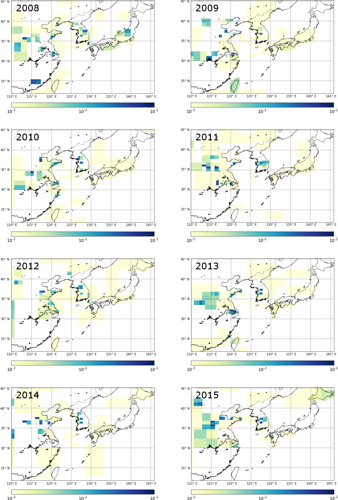
Figure 6 Emission maps for all years of data available for CF₄. Results are from inversions with initial uncertainty on the prior emission field set to 100 times the emissions at each fine grid square. Units are in g m⁻² yr⁻¹; see Fig. S7 for corresponding maps of emission magnitude minus the uncertainty.

CF₄

Our understanding of emissions of CF₄ and NF₃ is very poor, which is highlighted in global studies based on atmospheric measurements that show bottom-up estimates of emissions are significantly underestimated (Mühle et al., 2010; Arnold et al., 2013). With such a poor prior understanding of emissions, we assess the effect of prior uncertainty on the posterior emissions (Fig. 4). With assignment of uncertainty on the prior of each fine grid cell at 10 times the prior emission value, the posterior is still significantly constrained by the prior for both China and South Korea. When larger uncertainties are applied to the prior (100 times to 10 000 times), the posterior estimates are very consistent, indicating that when greater than 100× uncertainty is applied, emission estimates are most significantly constrained by the atmospheric measurements. For China, for 7 of the 8 years studied, our posterior estimates are greater than twice the prior estimates taken from EDGAR v4.2. The latest global estimates are from Rigby et al. (2014) and they estimated global CF₄ emissions of 10.4±0.6 Gg yr⁻¹ in 2008 with a steady but small increase to 11.1±0.4 Gg yr⁻¹ in 2013 (with the exception of a dip in 2009 to 9.3±0.5 Gg yr⁻¹). We highlight that our Chinese emission estimates remain within a narrow range for 5 of the 8 years studied at between 4.0 and 4.7 Gg yr⁻¹ (with typical uncertainties < 2.7 Gg yr⁻¹), and for 7 of the 8 years studied between 2.82 and 5.35 Gg yr⁻¹. However, the estimate for 2012 appears to be anomalous at 8.25±2.59 Gg yr⁻¹. In relation to the global top-down estimates from 2008 to 2012, our Chinese estimates represent between 37 and 45 % of global emissions between 2008 and 2011 with a jump to 74 % in 2012. This significant increase in 2012 is not reconcilable with atmospheric measurements on the global scale and is very likely a spurious result of the inversion. The most probable explanation for such a result is the incorrect assignment of emissions on the inversion grid. Incorrect assignment of emissions can occur between countries, particularly where air parcels frequently pass over more than one country, therefore reducing the ability of the inversion to confidently place emissions. However, there is not an obvious drop in emissions for another country in 2012 that would offset the large increase in the Chinese emission estimate. Within a country, incorrect assignment of emissions from an area closer to the receptor to an area further from the receptor will increase the calculated total emissions due to increased dilution in going from a near to a far source. Our inversion is susceptible to this effect as we only have one site for assimilation of measurements; two measurement sites, spaced apart and straddling the area of interest, would provide significantly more information to constrain the spatial emission distribution.

Our estimates are significantly higher than emission estimation methods using interspecies correlation: Kim et al. (2010) estimated CF₄ emissions in the range of only 1.7–3.1 Gg yr⁻¹ in 2008 and Li et al. (2011) only 1.4–2.9 Gg yr⁻¹ over the same period. The interspecies correlation approach inherently requires that the sources of the different gases that are compared are coincident in time and space. Kim et al. (2010) and Li et al. (2011) used HCFC-22 as the tracer compound for China with a calculated emission field from an inverse model, and most emissions of this gas originate from fugitive release from air conditioners and refrigerators. However, CF₄ is emitted mostly from point sources in the semiconductor and aluminium production industries with different spatial emission distribution within countries, and likely different temporal characteristics compared to HCFC-22.

Emission estimates from South Korea and Japan are 1 order of magnitude lower than those from China. For 2008, Li et al. (2011) estimate emissions of CF₄ from the combination of South and North Korea of 0.19–0.26 Gg yr⁻¹ and from Japan of 0.2–0.3 Gg yr⁻¹, which are on the low end of the uncertainty range of our estimates for that year (Table 1). As one of the largest, if not the largest, countries for semiconductor wafer production, Taiwan is also an emitter of CF₄. However, measurements at GSN provide only poor sensitivity to detection of emissions from Taiwan, and our results can only suggest that emissions are likely < 0.5 Gg yr⁻¹. North Korean emissions were small and no annual estimate was above 0.1 Gg yr⁻¹.

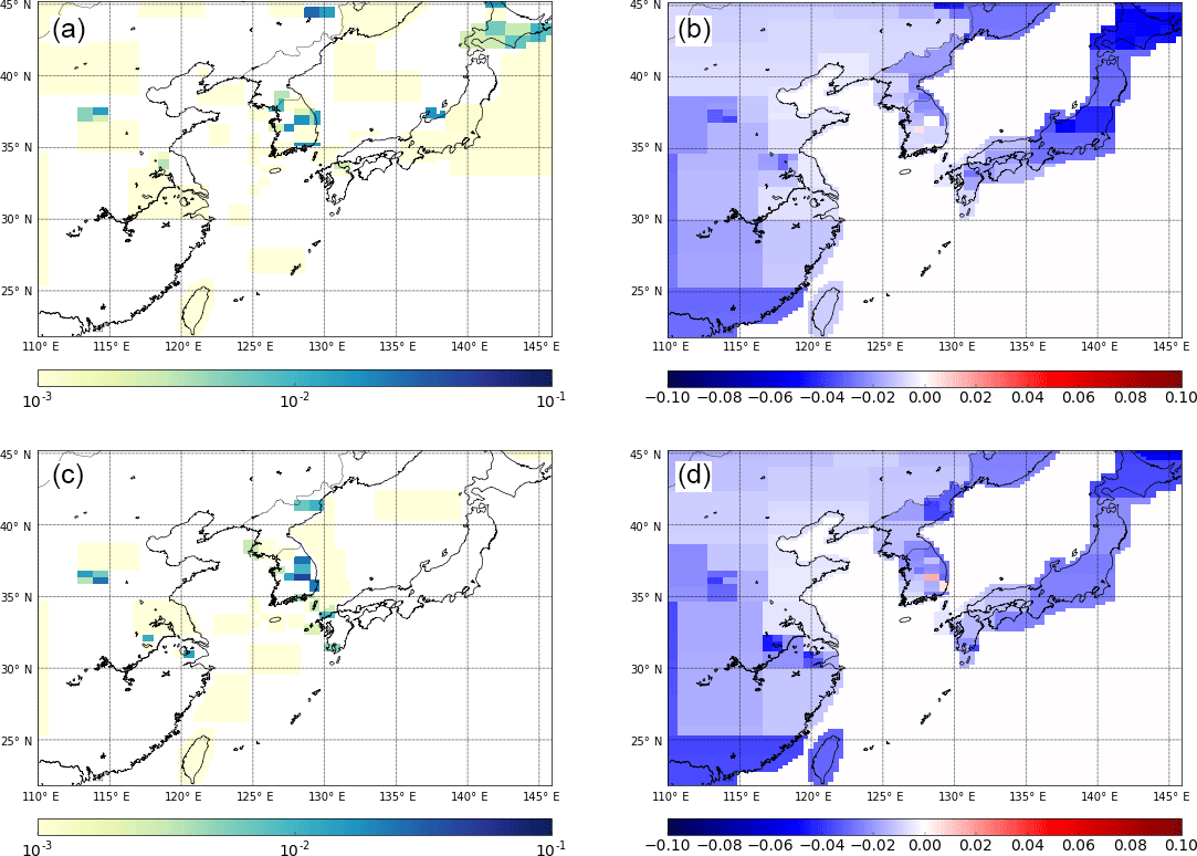
Figure 7 Emission maps for both years of data available for NF₃: panels (a) and (c) show posterior emission maps for the years 2014 and 2015, respectively. Panels (b) and (d) show the emission magnitude minus the uncertainty calculated for each inversion grid box for the years 2014 and 2015, respectively. Results are from inversions with initial uncertainty on the prior emission field is set to 100 times the emissions at each fine grid square. Units are in g m⁻² yr⁻¹.

Figure 8 As for Fig. 6 but for HFC-23.

NF₃

Our understanding of NF₃ emissions from inventory and industry data is even poorer than for CF₄. On a global scale, the emission estimates from industry are underestimated (Arnold et al., 2013). This study suggests that at least some emissions of NF₃ stem from China; however, gaining meaningful quantitative estimates has been difficult due to large uncertainties (Fig. 4). Contrastingly, the posterior estimates of emissions from South Korea have relatively small uncertainties. Emissions from China travel a greater distance to the measurement site compared to emissions from South Korea. Thus, the magnitudes of NF₃ pollution events from China (especially from provinces furthest west), in terms of the mixing ratio detected at GSN, are smaller than for pollution arriving from neighbouring South Korea. Also, the poorer measurement precision for NF₃ compared to CF₄ leads to a larger uncertainty on the baseline, which in turn affects the certainty on the pollution episode, especially for more dilute signals. Emission estimates for Japan are difficult to make without improved prior information and more atmospheric measurements in other locations. We argue that other large changes in our emission estimates from 2014 to 2015 could be real. For example, Japan's National Inventory Report for NF₃ shows a reduction in emissions of 63 % between 2013 and 2015 (Ministry of the Environment Japan et al., 2018), which is within the uncertainty of the relative rate of decrease we observe.

As for CF₄, emission estimates of NF₃ from Taiwan and North Korea are highly uncertain. However, our results do indicate that emissions of NF₃ from Taiwan might be lower than from South Korea despite very similar-sized semiconductor production industries. Focussing on the more meaningful estimates from South Korea, emissions of NF₃ in 2015 are estimated to be 0.60±0.07 Gg yr⁻¹ which equates to 9660±1127 Gg yr⁻¹ CO₂ eq. emissions (based on a GWP₁₀₀ of 16 100). This is ∼1.6 % of the country's CO₂ emissions (Olivier et al., 2017), thus making a significant impact on their total GHG budget. Further, given that the sources of NF₃ are relatively few, these emissions can be assigned to a small number of industries, potentially making NF₃ an easy target for focussed mitigation policy. Rigby et al. (2014) updated the global emission estimates from Arnold et al. (2013), and calculated an annual emission estimate of 1.61 Gg yr⁻¹ for 2012, with an average annual growth rate over the previous 5 years of 0.18 Gg yr⁻¹. Linearly extrapolating this growth to 2014 and 2015 leads to projected global emissions of 1.97 and 2.15 Gg yr⁻¹ for 2014 and 2015, respectively. Thus, South Korean emissions as a percentage of these global totals equate to ∼20 % and ∼28 % for 2014 and 2015, respectively, which is around the proportion of semiconductor wafer fabrication capacity in South Korea relative to global totals (∼20 %) (SEMI, 2017).

3.2 Spatial emission maps

We use “emissions minus uncertainty” maps (e.g. Fig. 5b) to provide information on where we are most certain of large emissions, i.e. where emission hotspots are located and if they are significant: less negative values indicate more certainty, with positive values indicating that the uncertainty is less than the best estimate and negative values indicating that the uncertainty is bigger than the estimate. A more common way to illustrate grid-level uncertainty is in an “uncertainty reduction” map. This works well when starting from a relatively well-constrained, spatially resolved prior to illustrate the additional constraint the atmospheric observations add. In this study, however, we are starting from very poor prior information and we generate a posterior emission map that is very distinct from the prior, informed largely by the measurements. Thus, an uncertainty reduction map provides little useful information.

Figure 5 shows the effect of regridding over the course of 50 separate CF₄ inversions (for 2015), from zero regridding steps (i.e. using a coarse grid space determined using information from NAME and the prior emissions), through to 25, and then 50 steps. The inversion was not allowed to decrease the minimum posterior grid size beyond four fine grid squares (i.e. 4 times the $\mathrm{0.3516}{}^{\circ }\times \mathrm{0.2344}{}^{\circ }$ grid square). This method highlights the areas that have the highest emission density; the splitting of these grid cells improves the correlation between observations and posterior model output. However, these emission maps must be studied alongside the corresponding uncertainty maps. The inversion could continue to split towards a fine grid resolution limit even though there may not be enough information in the data to accurately constrain emissions from each course grid cell (leading to spurious emission patterns) and the process would be computationally very expensive. The largest emissions of CF₄ arise from China, and Fig. 5 suggests the largest emissions come from an area between 35 and 38^∘ N. The uncertainty on these emissions from the specific final coarse grid squares is large, and therefore care needs to be taken not to overinterpret emission hotspots. Although the grid is being split, it is not realistic for the model to correctly interpret the spatial distribution of emissions at this distance from GSN, and this is demonstrated in Fig. 5f where the relative error on emissions in this corner of the domain is large. Without better prior information, it is not possible to distinguish between real year-to-year emission pattern changes and inaccurate emission patterns (Figs. 6 and S7). Over the period of study, emissions of CF₄ generally appear to arise from north of 30^∘ N, and in 2008 and 2013 emissions appear around 25^∘ N. However, GSN does not have good sensitivity to emissions from this area and it is possible that these emissions could be incorrectly assigned from Taiwan. Although emissions from South Korea are significantly lower than for China, the proximity to GSN causes the grid cells to be split and emissions to be assigned at higher spatial resolution and generally (except for 2008) in the north-west quadrant of the country. Splitting of grid cells in South Korea decreased the relative error on the emissions from particular grid squares, providing confidence that the placement of emissions is accurate. Further, for the sequential years 2013, 2014, and 2015, two specific grid cells in that north-west quadrant of South Korea are are highlighted with comparatively low uncertainties (Fig. S7). How well these consistent year-to-year emission patterns in South Korea correlate with the actual location of emissions needs to be the subject of further study (e.g. improved bottom-up inventory compilation efforts). Emissions from Japan are too uncertain to explore the spatial emissions pattern.

For NF₃, emissions from China and Japan are too low and uncertain to interpret at finer spatial resolution. However, as with CF₄, it is interesting to study the relatively more certain spatially disaggregated emissions from South Korea (Fig. 7). In common with CF₄, NF₃ emissions from the south-west area are minimal; however, in contrast to CF₄, emissions occur on the eastern side of South Korea and on the south-east coast. Emissions from the south-east coast coincide with the known location of a production plant for NF₃ located in the area of Ulsan (Gas World, 2011). If this plant is sufficiently separated in space from the end-users of NF₃, then this result would indicate that production of NF₃, not just use, could be a significant source in South Korea.

The study of Fang et al. (2015) highlights three major hotspots for HFC-23 emissions in China based on HCFC-22 production facility locations. Our posterior maps (Fig. 8) correctly show the bulk of emissions in far eastern China, in line with the results of Fang et al. (2015). However, given the inconsistency of emission maps between years, we are unable to provide any more information without a better spatially disaggregated prior emission map.

4 Conclusions

We largely remove the influence of bottom-up information and present the first Bayesian inversion estimates of CF₄ and NF₃ from the East Asian region using measurements from a single atmospheric monitoring site, GSN station located on the island of Jeju (South Korea). The largest CF₄ emissions are from China, estimated at 4–6 Gg yr⁻¹ for 6 out of the 8 years studied, which is significantly larger than previous estimates. Despite significantly smaller emissions from South Korea, the spatial disaggregation of CF₄ emissions was consistent between independent inversions based on annual measurement data sets, indicating the north-west of South Korea is a hotspot for significant CF₄ release, presumably from the semiconductor industry. Emissions of NF₃ from South Korea were quantifiable with significant certainty, and represent large emissions on a CO₂ eq. basis (∼1.6 % of South Korea's CO₂ emissions in 2015). HFC-23 emissions were also calculated using the same inversion methodology with high uncertainty on prior information. We found good agreement with other studies in terms of aggregated country totals and spatial emissions patterns, providing confidence that our methodology is suitable and our conclusions are justified for estimates of CF₄ and NF₃.

Our results highlight an inadequacy in both the bottom-up reported estimates for CF₄ and NF₃ and the limitations of the current measurement infrastructure for top-down estimates for these specific gases. Adequate bottom-up estimates have been lacking due to the absence of reporting requirements for these gases from China and South Korea, and top-down estimates have been hampered by poor measurement coverage due to the technical complexities required to measure these volatile, low-abundance gases at high precision. Improvements in both bottom-up information and measurement coverage, alongside refinements in transport modelling and developments in inversion methodologies, will lead to improved optimal emission estimates of these gases in future studies.