the Creative Commons Attribution 4.0 License.
the Creative Commons Attribution 4.0 License.
 | 12 Sep 2018
Simulated and observed horizontal inhomogeneities of optical thickness of Arctic stratus
Michael Schäfer
André Ehrlich
Corinna Hoose
Manfred Wendisch
Two-dimensional horizontal fields of cloud optical thickness τ derived from airborne measurements of solar spectral, cloud-reflected radiance are compared with semi-idealized large eddy simulations (LESs) of Arctic stratus performed with the Consortium for Small-scale Modeling (COSMO) atmospheric model. The measurements were collected during the Vertical Distribution of Ice in Arctic Clouds (VERDI) campaign carried out in Inuvik, Canada, in April/May 2012. The input for the LESs is obtained from collocated airborne dropsonde observations of a persistent Arctic stratus above the sea-ice-free Beaufort Sea. Simulations are performed for spatial resolutions of 50 m (1.6 km × 1.6 km domain) and 100 m (6.4 km × 6.4 km domain). Macrophysical cloud properties, such as cloud top altitude and vertical extent, are well captured by the COSMO simulations. However, COSMO produces rather homogeneous clouds compared to the measurements, in particular for the simulations with coarser spatial resolution. For both spatial resolutions, the directional structure of the cloud inhomogeneity is well represented by the model. Differences between the individual cases are mainly associated with the wind shear near cloud top and the vertical structure of the atmospheric boundary layer. A sensitivity study changing the wind velocity in COSMO by a vertically constant scaling factor shows that the directional, small-scale cloud inhomogeneity structures can range from 250 to 800 m, depending on the mean wind speed, if the simulated domain is large enough to capture also large-scale structures, which then influence the small-scale structures. For those cases, a threshold wind velocity is identified, which determines when the cloud inhomogeneity stops increasing with increasing wind velocity.
- Article
(4637 KB) - Full-text XML
- BibTeX
- EndNote


Arctic clouds are expected to be a major contributor to the so-called Arctic amplification (Serreze and Barry, 2011; Wendisch et al., 2017) and therefore need to be represented adequately in model projections of the future Arctic climate (Vavrus, 2004). Especially, low-level Arctic stratus are of importance (Wendisch et al., 2013), because they occur quite frequently (around 40 %; Shupe et al., 2006, 2011), typically persist over several days or even weeks (Shupe et al., 2011), and, on annual average, warm the Arctic surface (Shupe and Intrieri, 2004). The numerous physical and microphysical processes that determine the properties of Arctic stratus are complexly linked to each other (e.g., Curry et al., 1996) and still not understood in full detail (Morrison et al., 2012).
Dynamic factors (updrafts), which increase the actual supersaturation in the cloud beyond the equilibrium values for both liquid water and ice, and a steady supply of water vapor from above the cloud, stabilize Arctic stratus (Shupe et al., 2008). This facilitates the simultaneous existence and formation of both phases (Korolev, 2007). While in updrafts supercooled liquid water droplets and ice crystals grow, and the cloud top cooling causes downward vertical motion, the Wegener–Bergeron–Findeisen process may dominate. Therefore, small-scale structures may evolve in down- and updraft regions of the stratus, which can be important to understand the microphysical processes keeping the cloud persisting for a longer time period. Additionally, Arctic stratus shows microphysical inhomogeneities, which typically occur on horizontal and vertical scales below a few kilometers and even tens of meters (Chylek and Borel, 2004; Lawson et al., 2010). The small-scale cloud structures, which accompany cloud inhomogeneities, lead to three-dimensional (3-D) radiative effects (Varnai and Marshak, 2001), which can be parameterized using inhomogeneity parameters (Iwabuchi and Hayasaka, 2002; Oreopoulos and Cahalan, 2005).
Unfortunately, the understanding of Arctic cloud processes (e.g., longevity, precipitation formation) is impeded by a paucity of comprehensive observations caused by a lack of basic research infrastructure and the harsh Arctic environment (Intrieri et al., 2002; Shupe et al., 2011). Therefore, observation of small-scale cloud structures within the Arctic Circle are sparse. Satellite observations are typically too coarse to resolve scales below 250 m. Spaceborne passive remote sensing observations suffer from contrast problems over highly reflecting surfaces (snow and sea ice; Rossow and Schiffer, 1991; Ehrlich et al., 2017). Ground-based remote sensing measurements with radar and lidar typically point only in zenith direction and are not able to provide the horizontal two-dimensional (2-D) structure of clouds. Only along the wind direction the variability of clouds is resolved (Shiobara et al., 2003; Marchand et al., 2007). For example, using correlation analysis, Hinkelmann (2013) revealed significant differences between along-wind and cross-wind solar irradiance variability on small spatial scales in broken-cloud situations. In comparison, airborne spectral imaging observation of reflected solar radiation provides areal measurements with a spatial resolution down to several meters (Schäfer et al., 2015). Bierwirth et al. (2013) used such airborne measurements of reflected solar spectral radiance to retrieve 2-D fields of cloud optical thickness τ of Arctic stratus and demonstrated their strong spatial variability. From similar measurements, Schäfer et al. (2017a) analyzed the directional variability of different cloud types including Arctic stratus. The few analyzed cases revealed that one-dimensional (1-D) statistics are not sufficient to quantify the variability of horizontal cloud inhomogeneities.
Likewise, treating small-scale inhomogeneities using reanalysis data and atmospheric models is difficult. Global reanalysis products have relatively coarse spatial resolutions (40 km and larger; Lindsay et al., 2014) and therefore do not resolve small-scale features. Furthermore, in numerical weather prediction and climate models, the representation of the temporal evolution of mixed-phase clouds is not always adequate (Barrett et al., 2017a, b). Especially, areas of up- and downdrafts in Arctic stratus, which are typically in the range of less than 1 km, cannot be resolved but need to be parameterized (Field et al., 2004; Klein et al., 2009). To realistically simulate the spatial structure of these clouds, large eddy simulations (LESs) with a spatial resolution of 100 m or less and high vertical resolution (≈20 m within atmospheric boundary layer, ABL) are needed. Those LESs can resolve the vertical motion of the turbulent eddies in the ABL and the cores of up- and downdrafts representing the inhomogeneities in the cloud top structure, which can be seen in the amount of liquid water at the cloud top. The size of the up- and downdraft cores may differ depending on the time of the year (Roesler et al., 2016).
Previous LES studies focused, for instance, on cloud top entrainment (Mellado, 2017) and emphasized the behavior of changes in the spatial resolution on the liquid water path (Pedersen et al., 2016). Kopec et al. (2016) discussed two main processes: the radiative cooling and wind shear. The radiative cooling sharpened the inversion, while wind shear at the top of the ABL caused the turbulence in the capping inversion and led to dilution at the cloud top.
In general, LESs are helpful to focus on a certain process and to investigate cloud formation and evolution, or the small-scale structures in Arctic stratus under controlled conditions. Furthermore, horizontal small-scale cloud inhomogeneities in the size range of less than 1 km in simulations and measurements can be investigated with LES to better understand the radiative properties of Arctic mixed-phase clouds. In this paper, results from the Consortium for Small-scale Modeling (COSMO) model are evaluated, which is adjusted to an LES setup with a high horizontal and vertical resolution to resolve the cloud structures of Arctic stratus (Loewe et al., 2017; Stevens et al., 2018). For the Arctic Summer Cloud Ocean Study (ASCOS), Loewe et al. (2017) validated COSMO for simulations with a spatial resolution of 100 m with respect to droplet/ice crystal number concentrations, cloud top/bottom altitudes, and surface energy fluxes. Cloud structures and inhomogeneities were not validated due to the lack of observational data from ASCOS. In this paper, airborne imaging spectrometer measurements, obtained during the Vertical Distribution of Ice in Arctic Clouds (VERDI) campaign, are used to analyze small-scale cloud inhomogeneities (less than 1 km), which are then compared to COSMO simulations using the same model setup as proposed by Loewe et al. (2017) with 64 by 64 grid points and 100 m spatial resolution as well as a setup with higher resolution of 32 by 32 grid points and 50 m spatial resolution.
For that, data measured by dropsondes released by aircraft during VERDI served as input for semi-idealized simulations of clouds using COSMO-LES (Sects. 2.3 and 3). Airborne measurements performed during VERDI are used to retrieve fields of cloud optical thickness from imaging spectrometer measurements (Sect. 2.2). These fields compared with the COSMO results with respect to their overall cloud inhomogeneity and directional features of the cloud inhomogeneities (Sects. 4 and 5). Observations and modeling are aimed to quantify the horizontal cloud top structures, which are discussed in Sects. 5 and 6.

Figure 1Exemplary selected sections (1.2 by 3.0 km) of horizontal fields of τ to illustrate the daily variability of the horizontal cloud inhomogeneities during the VERDI campaign on (a) 14 May 2012, (b) 15 May 2012, (c) 16 May 2012, and (d) 17 May 2012. Data are adapted from Schäfer et al. (2017b).
2.1 Vertical Distribution of Ice in Arctic clouds (VERDI) campaign
Cloud remote sensing data and atmospheric profile measurements by dropsondes from the airborne VERDI campaign (Bierwirth et al., 2013; Schäfer et al., 2015, 2017a) are exploited in this study. VERDI was based in Inuvik, Canada, and was conducted in April/May 2012. The data were collected aboard the Polar 5 research aircraft of the Alfred Wegener Institute, Helmholtz Centre for Polar and Marine Research (AWI). The measurement flights were carried out in the region over the Beaufort Sea, which was mostly covered by sea ice, but also included sea-ice-free areas (polynyas). Mostly stratiform, low-level liquid and mixed-phase clouds within a temperature range of −19 to 0 ∘C were investigated (Costa et al., 2017). Here, the analysis is focused on a persistent cloud layer probed on 4 consecutive days from 14 to 17 May 2012. The applied measurements were performed in close vicinity (less than 50 km) over constant surface conditions (open ocean; polynyas). The persistent cloud cover in the respective area decreased continuously from day to day with cloud top altitude decreasing from about 880 m on 14 May to around 200 m on 17 May (Klingebiel et al., 2015; Schäfer et al., 2015, 2017a).
The Polar 5 research aircraft was equipped with a set of cloud and aerosol in situ and remote sensing instruments (Bierwirth et al., 2013; Schäfer et al., 2015; Klingebiel et al., 2015). Atmospheric profiles of temperature, humidity, wind speed, and direction were derived from dropsonde measurements, which were regularly released during all flights.
2.2 Horizontal fields of cloud optical thickness
The qualitative and quantitative description of the cloud inhomogeneities is performed using 2-D fields of cloud optical thickness τ. Marshak et al. (1995), Oreopoulos et al. (2000), and Schröder (2004) proposed to study horizontal cloud inhomogeneities using cloud top reflectances. However, Schäfer et al. (2017a) pointed out that radiance measurements include the information of the scattering phase function (e.g., forward/backward scattering peak, halo features). To avoid artifacts in the inhomogeneity analysis from such features, parameters that are independent of the directional scattering of the cloud particles have to be analyzed. Therefore, to characterize the observed and simulated cloud fields regarding their horizontal cloud inhomogeneities, the cloud optical thickness is applied, which does not include the fingerprint of the scattering phase function.
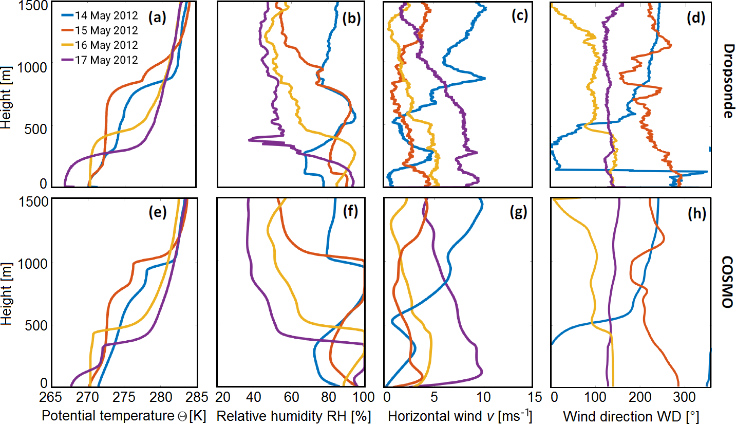
Figure 2(a, e) Potential temperature, (b, f) relative humidity, (c, g) wind speed, and (d, h) wind direction for the four investigated cases. The dropsonde data are shown in the first row (a–d) and the 2 h domain-averaged profiles after spin-up time of the simulations are shown in the second row (e–h). Dropsondes were released closest to the imaging spectrometer measurements.
The 2-D fields of τ are retrieved from 2-D fields of reflected solar spectral radiance, which were collected with the imaging spectrometer AisaEAGLE (Schäfer et al., 2013, 2015). Using those data, Schäfer et al. (2017a) retrieved 10 cases of 2-D fields of cloud optical thickness τ (Schäfer et al., 2017b). From those 10 cases, four are selected for the comparison with the LES results obtained from COSMO. Figure 1 illustrates selected sections (1.2 km by 3.0 km) of four cases. The full widths and lengths of the available 2-D fields of τ range from 1.7 to 26.8 km. Their spatial resolution is between 2.6 and 3.6 m (depending on the vertical distance between aircraft and cloud).
During the time period from 14 to 17 May 2012, the areal average of τ of the observed clouds decreased from 8.1 to 4.3 (compare Table 2, Schäfer et al., 2017a). The selected sections in Fig. 1 illustrate the temporal evolution of τ. In particular, from 15 to 17 May 2012, a reduction of the horizontal cloud inhomogeneity is visible, which is confirmed by Schäfer et al. (2017a), who also found a continuous reduction of cloud inhomogeneity during those 4 consecutive days. Furthermore, directional features, which are prominent on 14 May, seem to be reduced, which is also confirmed by Schäfer et al. (2017a).
2.3 Vertical profiles of atmospheric parameters
During each measurement flight, Vaisala dropsondes (type RD94) were used together with the Vaisala AVAPS (Airborne Vertical Atmosphere Profiling System) dropsonde receiving system (Hock and Franklin, 1999; Coleman, 2003). The dropsondes were released to sample profiles of meteorological parameters – air pressure (p), air temperature (T), relative humidity (RH), wind speed (v), and wind direction (WD) – below the aircraft, which typically operated at about 3 km altitude to sample the entire cloud and ABL structure. The accuracy of the dropsonde measurements is specified by the manufacturer as ±0.4 hPa for the air pressure, ±0.2 ∘C for the air temperature, ±2 % for the relative humidity, and ±0.5 m s−1 for the wind speed. The potential temperature (Θ), RH, v, and WD profiles for the four investigated cases are displayed in Fig. 2.
From 14 to 15 May, the cloud top inversion increased from 810 to 880 m, while for the subsequent 2 days, the inversion layer decreased to 440 m on 16 May and to 200 m on 17 May 2012 (Fig. 2a). In conjunction with the decrease of the cloud top altitude, the cloud base decreased as well until it almost reached the surface on 17 May. The relative humidity (Fig. 2b) confirms the initial increase and consecutive decrease of the cloud top and base altitudes. The inversion strength decreased over the time period from about 5 to 1 K mainly because the temperature of the surface layer continuously decreased; the ABL became more stable.
Figure 2c illustrates that the near-surface wind increased during the 4 days from about 1 to 10 m s−1. Except for the case on 14 May, the daily increase of the near-surface wind speed is observed as well in higher altitudes to up to 1 km. Following Jacobson et al. (2013), this is related to low-level jets (LLJs) for the days from 15 to 17 May.
3.1 COSMO: general setup
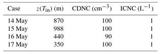
COSMO is a non-hydrostatic, limited-area atmospheric forecast model (Schättler et al., 2015). Here, it is used in a semi-idealized LES setup, which follows the description by Loewe et al. (2017), based on Ovchinnikov et al. (2014), and Paukert and Hoose (2014). The two-moment cloud microphysics scheme by Seifert and Beheng (2006) predicts the number densities and masses of six hydrometeor types. The different ice-phase hydrometeor growth processes are parameterized. The radiative transfer is described by a two-stream radiation scheme (Ritter and Geleyn, 1992). It is calculated every 2 s and has a direct cloud radiative feedback. A 3-D prognostic turbulence scheme describes the turbulent fluxes of heat, momentum, and mass by a first-order closure after Smagorinsky and Lilly (Herzog et al., 2002; Langhans et al., 2012). The horizontal size of the model domain used by Loewe et al. (2017) was 6.4×6.4 km with a spatial resolution of 100 m. Here, this setup is applied as well. However, analyzing cloud inhomogeneities requires a fine horizontal spatial resolution of the model simulations. Therefore, for the comparison with the imaging spectrometer measurements analyzed here, the spatial resolution is also increased to 50 m for addition model runs. In those cases, the domain size is reduced to 32 by 32 grid points (1.6 km × 1.6 km) for computational constraints. A further reduction of the spatial resolution was not possible due to numerical instabilities, probably caused by the propagation and growth of perturbations stemming from imbalanced initial and/or boundary conditions (Duran, 2010). The vertical height range of 22 km is divided into 166 levels, which are more dense for the ABL with a typical vertical resolution of around 15 m up to the inversion height of the different days of investigation. The initialization profiles of temperature, humidity, wind speed, and wind direction are based on the dropsonde data, which are partly affected by horizontal variability, when slowly passing the cloud and drifting horizontally. Therefore, parts of the original profiles (Fig. 2) are smoothed vertically for initialization of the model. The surface of the model is open ocean and the surface fluxes depend on the surface temperature, which is 273.5 K for the seawater surface. Moreover, ERA-Interim reanalysis data from the European Centre for Medium-Range Weather Forecasts (Dee et al., 2011) have been used to complete the profiles above the altitude where the dropsondes were released. Other model parameters include the description of the large-scale subsidence, which is adjusted to the temperature inversion height, the relaxation to fixed cloud droplet number concentration (CDNC), and ice crystal number concentration (ICNC). The spin-up time was set to 2 h following Ovchinnikov et al. (2014). The CDNCs are based on measurements of the Small Ice Detector (SID3; Vochezer et al., 2016). During the 4 investigated days, CDNCs of 90 to 100 cm−3 were observed as summarized in Table 1. The concentration of ice crystals was below or at the detection limit of the SID3. Therefore, the ICNC were assumed to be one particle per liter according to observations of mixed-phase Arctic stratus during the Indirect and Semi-Direct Aerosol Campaign (McFarquhar et al., 2011; Ovchinnikov et al., 2014). The inversion height of the temperature, z(Tin), is necessary for the description of the large-scale subsidence in the model and is represented by the inversion height of the dropsonde profiles, which are used for initialization of the simulations (Table 1).
Table 1Model setup specifications of the different mixed-phase cloud simulations of 4 VERDI campaign days.
3.2 Domain-averaged cloud properties and temporal evolution
Time series of simulated liquid water content (LWC) and ice water content (IWC) for the four selected cases are shown in Fig. 3. During the four considered flights, only few ice crystals were observed. The simulated clouds consisted mostly of liquid water droplets except for 15 May, in which more IWC was built at about 4 h after model initialization (Fig. 3b). Furthermore, the cloud top is around 1000 m for 14 and 15 May (Fig. 3a, b). However, the cloud top height increases over time in all four simulations because of entrainment of air through the top of the ABL. This is evident in the temporal evolution of LWC, which has a maximum between 0.25 and 0.35 g kg−1 near the cloud top. The Arctic clouds on 16 and 17 May are the lowest simulated clouds with a cloud top initially around 450 and 350 m, respectively (Fig. 3c, d).
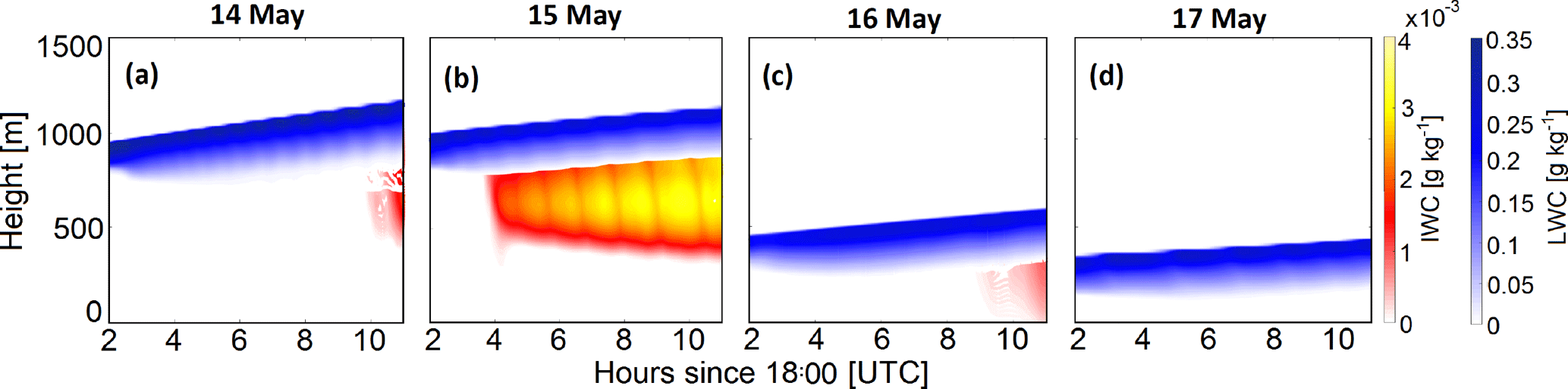
Figure 3Domain averages of LWC (blue color scale) and IWC (red–yellow color scale) of the four simulations during the VERDI campaign. Please note the different color scale for the IWC in panel (d).
The four simulations show differences in the temperature, relative humidity, and wind speed profiles (Fig. 2e–g), which in general still agree with the initial dropsonde profiles after the spin-up time (Fig. 2a–c). The height of the ABLs and the strength of the inversions are lower in the simulations of 16 and 17 May. Furthermore, for the simulation on 17 May, a second inversion develops in the ABL near the surface around 60 to 150 m. The ABL structure is well mixed in the simulation of 16 May although no second temperature inversion is built near the surface. The simulation of 16 May shows a wind shear from around 150 to around 100∘ (Fig. 2g) and a decrease of v with height above the cloud top height, which is also seen in the dropsonde profiles (Fig. 2c). The other simulations do not show a turning of the wind directly above the inversion height.
The simulated mixed-phase clouds of the four VERDI flights show a liquid water path (LWP) around 35 to 50 g m−2. The highest LWP is seen in the simulation of 14 May, which increases towards 50 g m−2 at the end of the simulation. The simulation of 15 May has the lowest LWP values. Furthermore, the LWP remains very stable until the end of the simulation. The ice water path (IWP) and the snow water path (SWP) of all four simulations are small, especially for the simulated clouds on 14, 16, and 17 May, which fits well with observations.
For the comparison of the simulated and observed horizontal cloud structures (cloud inhomogeneities), fields of simulated cloud optical thickness (τsim) are compared to retrieved fields of cloud optical thickness from the measurements (τmeas). The τsim is calculated within the COSMO model considering the amount of liquid water and the solar spectrum. However, it cannot be expected that COSMO is capable of reproducing the detailed spatial and temporal cloud evolutions, which are captured by the observed fields of τ, accurately (inhomogeneity features and directional structures). Therefore, besides the comparison of observed and simulated clouds with regard to macrophysical cloud features (cloud vertical extent, cloud optical thickness) of the individual cases, instead of point-by-point comparisons of cloud parameters, statistical bulk parameters describing the horizontal cloud inhomogeneities, their directional structures, and the temporal evolution of both will be compared.
4.1 One-dimensional statistical bulk parameters
For the quantitative description of the cloud inhomogeneities from the simulated fields of cloud optical thickness (τsim) obtained from COSMO and measurement-based retrieved fields of cloud optical thickness (τmeas) collected during the VERDI campaign, statistical techniques are applied. Following Schäfer et al. (2017a), different statistical quantitative measures of the cloud inhomogeneities are derived using the mean and standard deviation of the particular τ field and three 1-D inhomogeneity parameters: ρτ (Davis et al., 1999; Szczap et al., 2000), Sτ (Davis et al., 1999; Szczap et al., 2000), and χτ (Cahalan, 1994; Oreopoulos and Cahalan, 2005). They are given by
A homogeneous cloud is characterized by ρτ=0 and Sτ=0. Higher values of ρτ and Sτ indicate more pronounced cloud inhomogeneity. However, both of them have no predefined upper limit. Therefore, ρτ and Sτ only sustain a quantitatively significance, when their values for different cases are compared to each other. The 1-D inhomogeneity parameter χτ ranges between 0 and 1, with values close to unity indicating horizontal homogeneity and values approaching zero characterizing high horizontal inhomogeneity. Due to the limited range between 0 and 1, χτ is not only a qualitative but also quantitative measure.
4.2 Two-dimensional autocorrelation analysis
Two-dimensional autocorrelation analysis is applied to quantify the typical scales of cloud inhomogeneities and to identify directional patterns of the cloud structures (Schäfer et al., 2017a). To derive the autocorrelation functions, each field of τ is correlated with itself, while it is shifted pixel by pixel (observations) or grid point by grid point (simulations) against itself. The values of the resulting correlation coefficients after each shift are in the range between −1 (perfect negative correlation) and 1 (perfect positive correlation). Correlation coefficients with values of 0 identify no correlation. Here, only the degree of correlation matters and not if it has a positive or negative sign. Similar to Schäfer et al. (2017a), squared autocorrelation functions are used to avoid ambiguous interpretations. The reach values between 0 (no correlation) and 1 (perfect correlation).
The particular correlation coefficients at the derived distances identify the similarity of the horizontal cloud structures. If the cloud is horizontally homogeneous, the correlation coefficients stay constant over large distances. If the cloud is rather inhomogeneous, the correlation coefficients already drop at closer distances. Therefore, as a function of distances is a measure of the size of the dominant cloud structures.
A quantitative value for the distance, at which cloud structures are different from each other (namely decorrelated), is the decorrelation length ξτ (Schäfer et al., 2017a). It is the distance, at which drops to
In a 2-D autocorrelation function, ξτ can differ depending on the orientation, if the cloud structures have a predominant orientation. To quantify this directionality, ξτ is calculated along () and across () the predominant direction. The larger the differences between and , the more cloud structures are orientated.
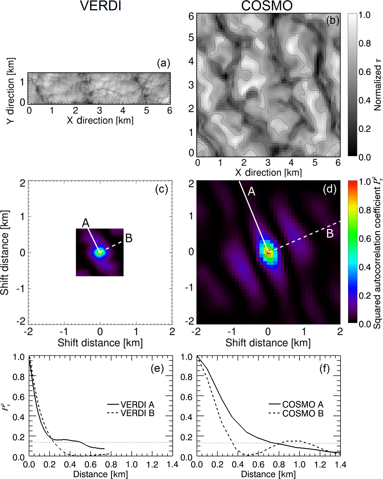
Figure 4(a–b) Horizontal fields of normalized τmeas (VERDI) and τsim (COSMO) for the case on 15 May 2012. (c–d) Two-dimensional autocorrelation coefficients and , calculated for fields of τ displayed in panels (a) and (b). (e–f) One-dimensional autocorrelation coefficients along (straight white line marked in panels c and d) and across (dashed white line marked in panels c and d) predominant directional structure. The grey dotted line illustrates the threshold for the estimation of and .
Figure 4a shows a section of an observed field of τmeas, retrieved from the measurements on 15 May. The selected section has a swath of 1.3 km (oriented in y direction) and a length of 6 km (oriented in x direction). Figure 4b shows the corresponding field of τsim (6 km × 6 km, adapted to the selected length of the measurement case), which is simulated with COSMO 2 h after the spin-up time for the case of 15 May. For comparability reasons, both fields of τ are normalized by their maximum.
Although the swath (y direction) of the field of τmeas is smaller by a factor of almost 5 compared to the field of τsim, larger cloud structures of similar size and shape are obvious in both fields of τmeas and τsim. However, with 488 spatial pixels along the swath (spatial double binning was applied during measurements) and a field of view of 37∘, AisaEAGLE's spatial resolution is approximately 1.3 m for a target in a distance of 1 km. Thus, the spatial resolution of AisaEAGLE is relatively high, compared to the spatial resolution of 100 m from COSMO. Thereby, the exact pixel size of AisaEAGLE depends on the distance between aircraft and cloud, which leads to pixel sizes between 2.6 and 3.6 m for the four investigated cases. Due to the 30 to 40 times higher spatial resolution of AisaEAGLE, compared to COSMO, the measurements show cloud features, which cannot be resolved by COSMO. Those features on a spatial scale below 100 m may have an effect on the statistical (1-D inhomogeneity parameters) and spatial comparison (autocorrelation analysis) of the particular fields of τ.
To quantify the size and orientation of the represented cloud structures in the observations and simulations, Fig. 4c and d show the calculated squared 2-D autocorrelation coefficients . To calculate them, different numbers of legs (shifts) have to be applied for and . The applied field of τmeas consists of 2700 by 450 spatial pixels. Therefore, restricted by the shorter side, 225 by 225 (half of swath pixel number, calculated into x and y direction) legs are chosen for the calculation of the 2-D . The COSMO results consist of 64 by 64 grid points. This allows 32 by 32 legs for the calculation of .

Figure 5Illustrated are sections of one and the same field of τmeas from 14 May 2012 with a spatial resolutions of (a) ≈3 m (original resolution), (b) 50 m (COSMO resolution), (c) 100 m (COSMO resolution), (d) 150 m, and (e) 300 m. (f–j) Squared 2-D autocorrelation coefficients calculated for the fields of τmeas displayed in panels (a) to (e). (k–o) Squared 1-D autocorrelation coefficients calculated along straight red line in panels (f) to (j). Estimated decorrelation length ξτ is marked by horizontal and vertical black lines and labeled by its value. Red dot marks ξτ as derived from the case with the original spatial resolution of 3 m.
The resolved domains and spatial resolutions, which are displayed in Fig. 4c and d, show significant differences, which reveals that a direct comparison is difficult. Applying the 2-D autocorrelation analysis to the observations allows to resolve small-scale cloud structures with high spatial resolution (approximately 2.7 m) but only within a narrow spatial range below 1 km. Contrarily, the same analysis for COSMO delivers with lower spatial resolution of 100 m but over a larger spatial range (about 3.2 km, in Fig. 4d only displayed until 2 km). Thus, also large-scale cloud structures are covered by COSMO (purple stripes in Fig. 4d) but not in the observations. Therefore, the large-scale structures cannot be compared between observations and simulations. With respect to a comparison of the small-scale structures, the spatial sizes (spatial resolution, domain size) of both data sets need to be conformed to make a direct comparison possible.
Furthermore, both Fig. 4c and d show predominant directional features of the cloud structures. Their lengths and widths are derived from 1-D autocorrelation functions along (straight white line in Fig. 4c and d) and across (dashed white line in Fig. 4c and d) those predominant directional structures and a subsequent estimation of and . The derived and show an overall agreement but still differ from each other. For the observations, and reach distances of approximately 500 and 250 m, respectively. Contrarily, for the simulations, and reach distances of approximately 800 and 400 m, respectively. This is a further indication that it is necessary to make the fields of τmeas and τsim conform with respect to their spatial resolution and domain. In the following, this is done by (i) averaging the observed fields of τmeas to the spatial resolution of the simulated fields of τsim and (ii) improving the spatial resolution of the simulations themselves.
Figure 4e and f further illustrate that it is not possible to compare the large-scale structures between observations and simulations. The large-scale structures, which are covered by the COSMO simulations, are identified by a second increase of the at distances (at approximately 1 km in Fig. 4f) larger than ξτ. The width of the measured fields is too narrow to cover such a second increase in the (compare Fig. 4e). Therefore, the further comparison of the cloud structures, which are identified in the observations and simulations, is restricted to the small-scale cloud structures with sizes below 1 km only.
4.3 Final data preparation – adjustment of spatial resolution and domain
To compare both data sets, the fields of τmeas, which are retrieved from the imaging spectrometer measurements, are averaged to the spatial resolution of the COSMO τsim fields. The investigations of the single cases during VERDI are performed for spatial resolutions of 50 m (32 by 32 grid points) and 100 m (64 by 64 grid points). All other model parameters are kept constant with respect to the analysis performed by Loewe et al. (2017).
In order to average the observed fields of τmeas to the spatial resolution of 50 and 100 m, the τmeas values of distinct numbers of neighboring pixels are averaged. The number depends on the single pixel size of the particular cases, which is a function of the vertical distance between aircraft and cloud. For the four investigated cases, this number varies between 13 (26) and 18 (36) pixels, which are needed to generate pixel sizes of τmeas comparable to the 50 m (100 m) spatial resolution of COSMO.
Furthermore, for the simulations with 100 m spatial resolution, the domain sizes of the measurements and simulations need to be adapted. The applied COSMO domain size of 6.4 km by 6.4 km is about 3 to 4 times larger than the domain size of the measurements. Therefore, to compare both data sets, the COSMO domain size is also reduced to the width and length of the corresponding τmeas field from the measurements. Therefore, for the comparison, only a squared domain in the center of COSMO's τsim field is used, whose size corresponds to the size of the particular field from the measurement. For the four investigated cases, this results in COSMO domains composed out of 12 by 12 to 16 by 16 grid points (1.2 km by 1.2 km to 1.6 km by 1.6 km). Longer stripes of τmeas fields and stripes according to their lengths across the COSMO domain are not used, because the investigations are focused on small-scale cloud inhomogeneities, which are already covered by the smaller squared domain size given by the swath of the τmeas fields.
For the COSMO simulations, which use 50 m spatial resolution, the domain size is reduced to 32 by 32 grid points, resulting in a total domain of 1.6 km by 1.6 km, which is comparable to the observations. Therefore, the domain of those simulations is not adapted for the comparisons.
However, to increase the statistics, which might be otherwise too small because of the finally applied small domain but large pixel sizes, for COSMO, averages of the resulting over all output time steps after spin-up are used. For the measured fields, whose lengths are much longer than their widths, squared domains (size determined by swath of τmeas) are cut along the measured stripe and the resulting values are averaged accordingly. Increasing the number of available , which can be used for averaging, is a further reason to use squared domains instead of stripes.
To test possible effects arising from the change of spatial resolution and to check if the relevant scales of cloud inhomogeneity are lost, when reducing the resolution of the measurements, Fig. 5a–e show sections of one and the same field of τmeas from the case of 14 May but displayed with a different spatial resolution of 3 m (original resolution), 50 m (COSMO fine resolution), 100 m (COSMO original resolution), 150 m, and 300 m resolution. Figure 5f–j show the corresponding squared 2-D autocorrelation coefficients. The red line illustrates the direction which is used to calculate the squared 1-D autocorrelation functions and decorrelation lengths ξτ, displayed in Fig. 5k–o. The fields from the 2-D autocorrelation analysis show that, except for the spatial resolution of 300 m, the directional structure of the cloud inhomogeneities is still captured, when the spatial resolution is reduced. However, the decorrelation lengths, derived from the 1-D autocorrelation analysis, increase with decreasing spatial resolution from ξτ=327 m at 3 m spatial resolution to ξτ=600 m at 300 m spatial resolution. Therefore, decreasing spatial resolution leads to larger ξτ, which indicates larger cloud structures. This means that reduced spatial resolution will generate fields of τ with larger spatial scales.
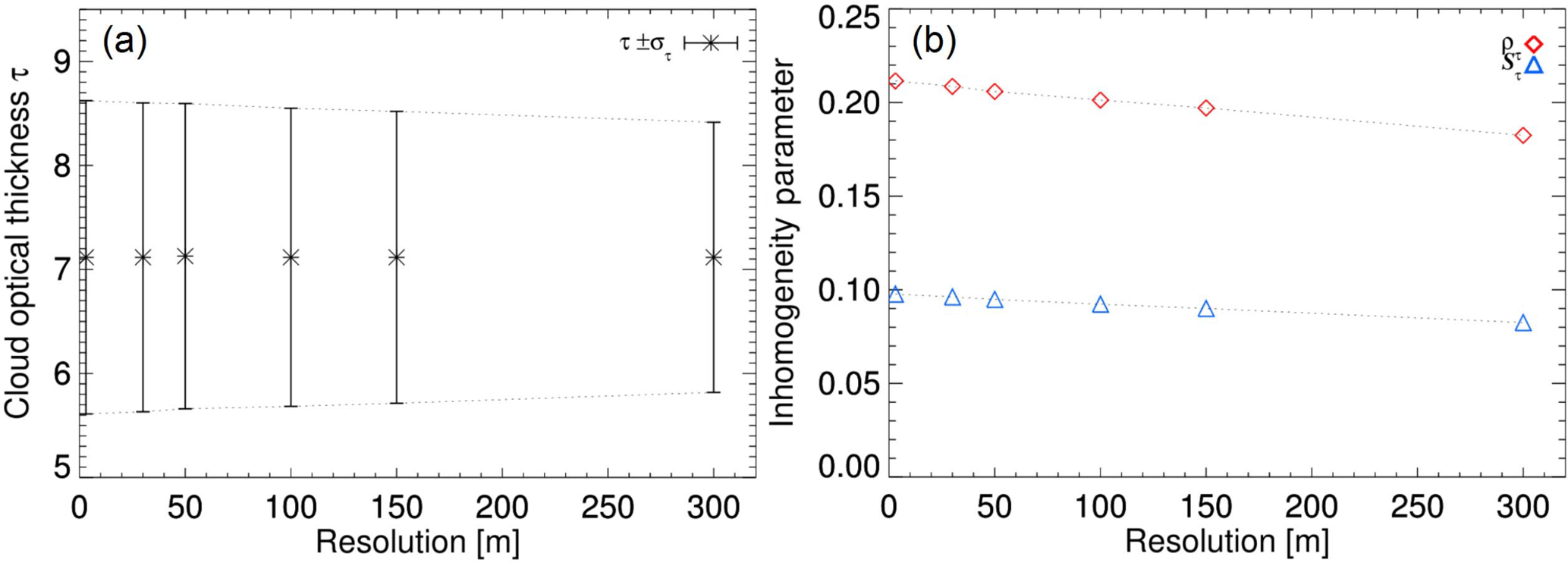
Figure 6Comparison of (a) mean and standard deviation and (b) inhomogeneity parameters (ρ and S) as a function of spatial resolution for the fields of τmeas illustrated in Fig. 5a–e.
To test the influence of the spatial resolution on the overall inhomogeneity, Fig. 6a shows the results for the mean and standard deviation of the fields of τ, illustrated in Fig. 5. Figure 6b shows the corresponding 1-D inhomogeneity parameters (ρτ and Sτ). While the mean value of τ stays constant for all spatial resolutions, its standard deviation decreases with increasing pixel size. This indicates that the fields of τ become more homogeneous the larger the pixel size is. Similarly, the values of both 1-D inhomogeneity parameters (ρτ and Sτ) decrease with increasing pixel size.
Therefore, in the following analysis, comparing the simulated against observed fields of τ, the simulations with the finer spatial resolution of 50 m are used. The simulations with 100 m spatial resolution are used to discuss the model sensitivity with respect to the spatial resolution.
5.1 Magnitude of inhomogeneity
The fields of τ obtained from the spectral imaging remote sensing (τmeas) are compared to the fields of τ derived from the COSMO simulations (τsim). To validate the cloud inhomogeneity in the simulated fields, the statistical techniques from Sect. 4.1, including the averaging of the measured fields to 50 and 100 m pixel size, are applied. Table 2 lists the mean values of τ, standard deviation στ, and the three 1-D inhomogeneity parameters (ρτ, Sτ, and χτ) for the observations and the simulations with the two different spatial resolutions of 50 and 100 m.
Table 2Mean value of τ, standard deviation στ, and the three 1-D inhomogeneity parameters (ρτ, Sτ, and χτ) calculated for all four cases from the observations and the simulations with the two different spatial resolutions of 50 and 100 m.
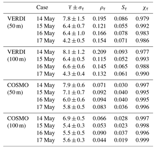
Both measurements and simulations show the highest areal averaged cloud optical thickness on 14 May with and at 50 m spatial resolution and and at 100 m spatial resolution, which indicate an overall agreement. During the course of the following days, the large-scale subsidence led to a decrease of the cloud top altitude and cloud geometrical thickness and corresponding lower values of τ and στ. For these days, the model and observations are still in agreement. However, compared to the spatial resolution of 100 m, it is obvious that the finer resolved simulations lead to better agreement between measurements and simulations.
Regarding the cloud inhomogeneity, the absolute values of the 1-D inhomogeneity parameters (ρτ, Sτ, and χτ) do not compare well for the simulations with 100 m spatial resolution. The results for the COSMO simulations show lower 1-D inhomogeneity parameters (more homogeneous) by a factor of 2 and higher, compared to the results from the measurements. The agreement between the observations and simulations increase with the finer spatial resolution of 50 m but still does not match perfectly. The reason might be that the comparably lower inhomogeneity derived from COSMO for both spatial resolutions is caused by its effective spatial resolution, which is approximately three times 50 m or accordingly three times 100 m (Skamarock, 2004). Although the pixel size of AisaEAGLE is adapted to the COSMO spatial resolution by averaging over neighboring pixels, COSMO's effective spatial resolution is larger, which might lead to larger homogeneity of the simulations compared to the observations. Furthermore, COSMO simulates the cloud at the same location where it is initialized. Contrarily, the AisaEAGLE measurements took place along a stripe of several kilometers. The simulated clouds may not change in between the time steps as much as the measurements of the clouds along the measurement stripe do. Therefore, averaging over COSMO's time steps might further produce more homogeneous results than averaging over AisaEAGLE's squared domains along the flight track.
However, the observations show that the cloud field became more homogeneous from 14 to 15 May as indicated by lower values of ρτ, which reduce from 0.209 to 0.115. From 15 to 16 May, ρτ increases to 0.145, which indicates a cloud field with slightly higher inhomogeneity. Then, on 17 May, ρτ reduced to 0.132, showing that the cloud field became more homogeneous again. These different cases with high and low ρτ are reproduced by COSMO independent of the chosen spatial resolution. Larger discrepancy between modeled and observed inhomogeneity parameters only occurred on 14 May, when the observations were influenced by large-scale cloud structures.
Nevertheless, the lower/higher inhomogeneity is also imprinted in the inhomogeneity parameters (Sτ and χτ), which are smaller/larger in both measurements and simulations, indicating that COSMO performs well with regard to the 1-D inhomogeneity parameters.
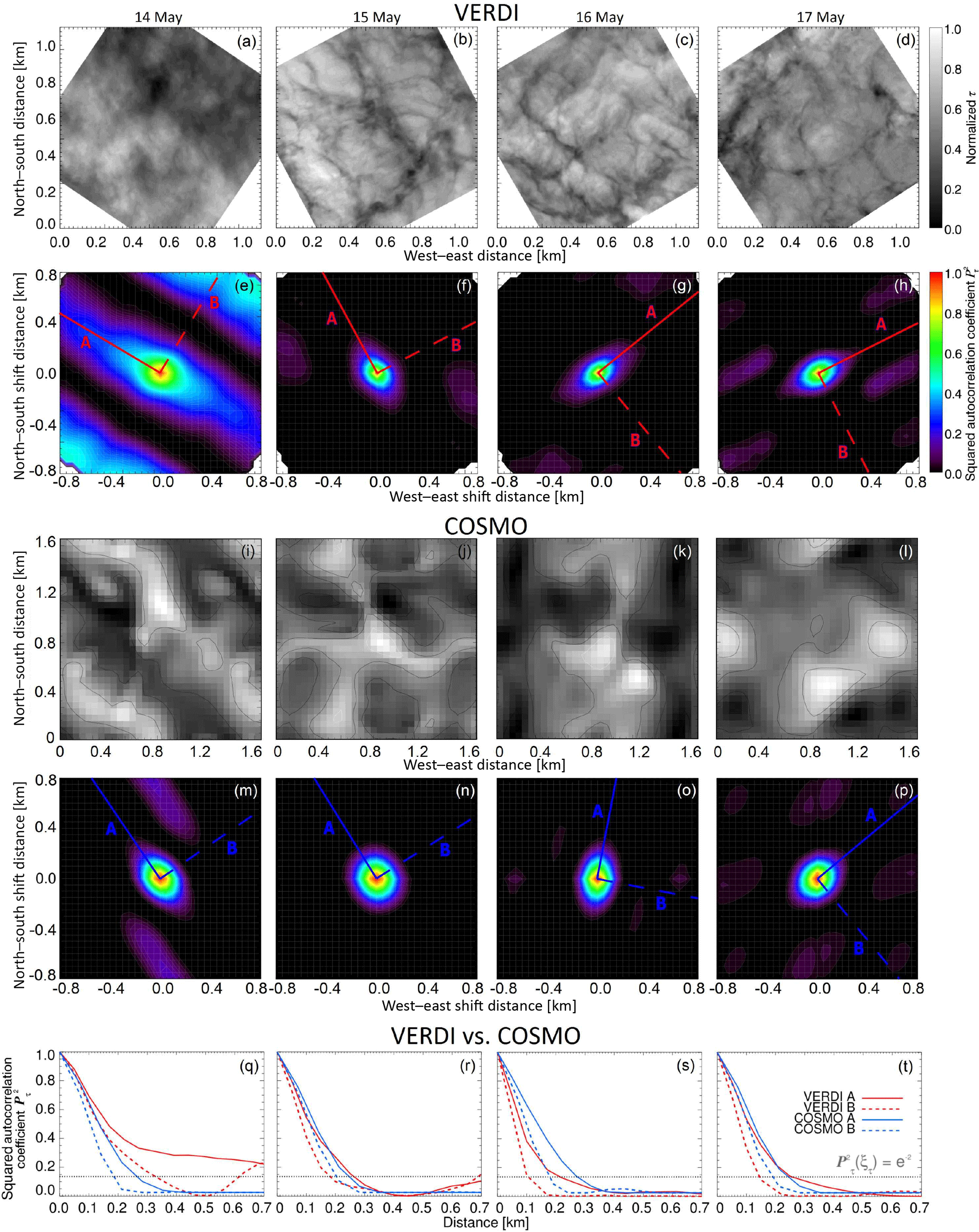
Figure 7(a–d) Exemplary selected sections of fields of τmeas observed during VERDI from 14 to 17 May 2012. (e–h) Mean 2-D autocorrelation coefficients derived for fields of τmeas from VERDI. (i–l) Exemplary selected fields of τsim simulated with COSMO (50 m spatial resolution) for the VERDI cases from 14 to 17 May 2012. (m–p) Mean 2-D autocorrelation coefficients derived for fields of τsim. (q–t) Decorrelation length ξτ along strongest (straight blue and red lines) and weakest (dashed blue and red lines) extents of 2-D autocorrelation coefficients derived from in panels (e)–(h) and in panels (m)–(p), respectively.
5.2 Spatial inhomogeneity scale
The 2-D autocorrelation functions are calculated to compare the typical spatial scales and the directional character of the small-scale cloud inhomogeneities (no large-scale inhomogeneities like roll convection) of observations and simulations. The 2-D autocorrelation coefficients (; ) for each case are shown in Fig. 7e–h for the measurements and in Fig. 7m–p for the simulations (50 m spatial resolution). Additionally, representative fields of normalized τmeas (Fig. 7a–d) and τsim (Fig. 7i–l) are added. The 2-D autocorrelation analysis was applied to the simulated fields of τsim orientated in a north–south and west–east grid. The orientation of the observations is determined by the flight direction. Therefore, the orientation of the fields of τmeas and are rotated into the direction of the COSMO grid. One-dimensional values are calculated manually along the dominant direction (straight red and blue lines in Fig. 7e–h and m–p) and across it (dashed red and blue lines in Fig. 7e–h and m–p). For (red) and (blue), the results are displayed in Fig. 7i–l. The dotted black line illustrates the threshold for the estimation of ξτ.
The observations on 14 May are influenced by a large-scale cloud structure, which is caused by large-scale dynamic forcing and leads to an increase of the autocorrelation coefficients for distances larger than 800 m. Furthermore, during this day, a significant directional structure from northwest to southeast is observed. Along this direction, the cloud field stays homogeneous over a wide range (ξτ=800 m). Across this predominant structure, the small-scale cloud structures reach a decorrelation length of ξτ=300 m. During the following days, the orientation of the directional structure turns eastwards in the observations. The differences between and decrease. This characterizes a weakening of the directional structure of the cloud field.
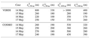
Table 3Calculated decorrelation lengths ξτ,meas and ξτ,sim for the two different spatial resolutions of 50 and 100 m along () and across () the observed and simulated predominant directions (compare Fig. 7e–h and m–p for 50 m spatial resolution).
Comparing the results for with reveals that the large-scale cloud structure is not well simulated for the case of 14 May. This results most probably from the small domain size of COSMO, which is fixed over the same location, when averaging the over a set of time steps. Contrarily, the averages of from the measurements are performed over a set of squared domains along the flight track. Thus, the chance to cover also larger structures is higher for the measurements compared to the simulations. However, the overall small-scale directional structures are well simulated. On 14 May, a significant directional structure from northwest to southeast is observed, which then turns eastwards for 15 to 17 May. Except on 16 May, the predominant simulated directions of the cloud fields are almost identically to the observations.
Furthermore, the results for and show that COSMO simulations using a spatial resolution of 50 m produce similar sizes of the small-scale cloud structures compared to the measurements. In Fig. 7m–p, the covered areas of are of similar sizes compared to the areas covered by in Fig. 7e–h. Table 3 lists the resulting ξτ,meas and ξτ,sim calculated along () and across () the predominant structures found in Fig. 7e–h and m–p. A comparison reveals only minor differences between ξτ,meas and ξτ,sim. The best agreement is achieved on 15 and 17 May, when ξτ,meas and ξτ,sim show almost identically results. On 16 May, the differences are slightly larger, while on 14 May the differences are significantly larger, which might result from the insufficient simulated large-scale cloud structure. For the simulations with 100 m spatial resolution (graph not shown), the directional features still compare well between observations and simulations. Like for the measurements on 14 May, a predominant northwest to southeast direction is simulated, which then turns eastwards. Thereby, the cases on 14 May and 16 May show the strongest directional features (largest differences between and , compare Table 3) with on 14 May larger than the width of the observed field of τmeas. Although on 17 May COSMO simulates a more isotropic structure ( m) of the cloud inhomogeneities compared to the measurements (), it captures the reduction of the overall directionality. Therefore, the overall results with regard to the directional structure provided by COSMO are acceptable. However, the covered areas of the 2-D autocorrelation functions, where the values of are higher than e−2 are larger compared to the areas covered by the particular . Therefore, the ξτ,meas and ξτ,sim calculated along () and across () the predominant structures do not compare well (compare Table 3). Like expected from Fig. 5, the values from the simulations (except for on 14 May) are larger compared to the values from the observations by 20 % to 30 %.
The reasons for the differences on 16 May (Fig. 7s) are most probably related to the wind field and the temperature profile. Figure 2d and h illustrate the temporally averaged wind directions in the simulations. While the wind direction does not change at the cloud top on 14, 15, and 17 May, the simulation of 16 May shows a turning of the wind. Together with the well-mixed ABL (Fig. 2), this case shows a typical example of a cold air outbreak roll convection (e.g., Brümmer, 1999). On 16 May, the simulated wind speed is significantly higher compared to the other days, resulting from the initial conditions in the dropsonde profile (Fig. 2c, d). Influences from the surface fluxes are only expected if the cloud is coupled to the surface and if so, affect only the LWP of the cloud (Loewe, 2017). For decoupled clouds, it is assumed that the cloud structure depends more strongly on the wind shear, respectively, the wind speed. However, since the wind speed, wind direction, and temperature profile are the only parameters, which have been changed in the model input, the wind speed and wind shear are expected to be main drivers for the degree of horizontal cloud inhomogeneity.
To test its influence on the horizontal cloud inhomogeneity, the simulations for 15 May (50 and 100 m spatial resolution) are repeated for different initializations, where the wind profile is varied. Here, the case on 15 May is chosen, because it shows the best agreement between observations and simulations (Fig. 7r) to serve as a benchmark case. Based on the original wind profile, the wind speeds at each altitude are multiplied by (a) 0.5, (b) 1.0, (c) 1.5, (d) 2.0, (e) 2.5, and (f) 3.0. This leads to mean wind speeds (vertically averaged over cloudy region) of approximately (a) 0.7 m s−1, (b) 1.5 m s−1, (c) 2.2 m s−1, (d) 3.0 m s−1, (e) 3.7 m s−1, and (f) 4.4 m s−1. The wind shear was kept constant throughout all simulations.
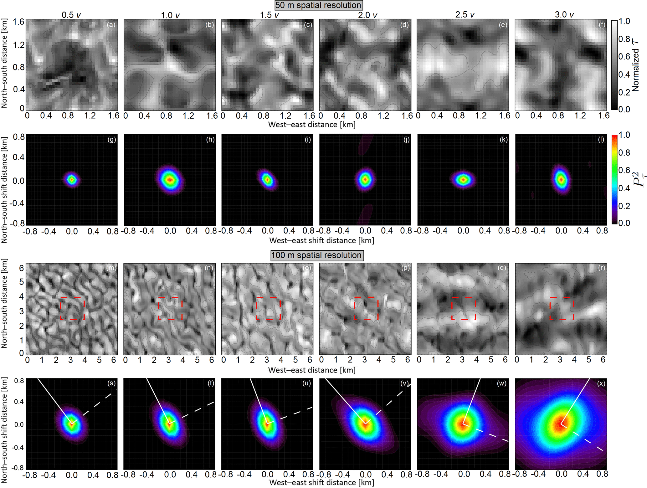
Figure 8Exemplary selected fields of τsim for the 15 May 2012 case simulated for differently scaled initial wind speeds on a grid with 50 m spatial resolution and 1.6 km by 1.6 km domain (a–f) and on a grid with 100 m spatial resolution and with 6.4 km by 6.4 km domain (m–r). Calculated 2-D autocorrelation coefficients are given for each case in panels (g)–(l) and (s)–(x). White lines in panels (s)–(x) illustrate the orientation used for the calculation of the 1-D along (straight white lines) and across (dashed white lines) the dominant directions illustrated in Fig. 9. Red squares in panels (m)–(r) mark areas of comparable size to the small domains in panels (a)–(f).
Figure 8a–f show the simulated 2-D fields of τsim for the simulations with the domain size of 1.6 km by 1.6 km and 50 m spatial resolution. Small-scale structures (smaller than 0.5 km) are obvious and rather randomly orientated throughout the simulations for all six different initializing wind profiles. The spatial sizes of the small-scale structures quantified by the decorrelation length depend only little on the wind speed. This is confirmed by the 2-D autocorrelation analysis, illustrated in Fig. 8g–l. Displayed are only the horizontal scales below 0.8 km, quantified by the 2-D autocorrelation coefficients for shifts smaller than ±0.8 km. A predominant direction of the small-scale structures is only slightly developed and varies independently from case to case without clear preference. Furthermore, the and the decorrelation length, which vary between 150 and 300 m show only slight variations with changing wind speeds. This means that the sizes of the small-scale structures are basically independent of the wind speed.
Contrarily, the simulations with a domain size of 6.4 km by 6.4 km and 100 m spatial resolution show a clear dependency on the wind speed. The corresponding 2-D fields of τsim are illustrated in Fig. 8m–r. The small-scale structures (smaller than 0.5 km) are still obvious in the simulations with coarse resolution. However, for a lower wind speed, these small-scale structures have a northwest to southeast orientation, which turns into northeast to southwest orientation with increasing wind speed. Additionally, large-scale structures (larger than 2 km), orientated perpendicular to the small-scale structures occur at 2.5 times the initial wind speed. The direction of these large-scale structures turns as well and becomes more obvious with increasing wind speed.
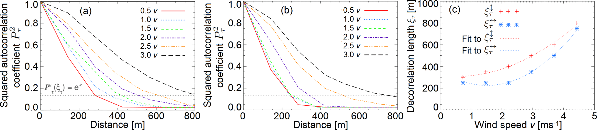
Figure 9The six cases of different wind speed calculated 1-D autocorrelation functions (a) along and (b) across the main structures are identified in Fig. 8g–l. The grey dotted line marks the threshold of . (c) From (a) and (b) derived discrete values for the decorrelation lengths and as a funktion of wind speed v (symbols). Additionally included are fits derived from Eqs. (5) and (6) (dotted lines).
The results for the 2-D autocorrelation analysis are given in Fig. 8g–l. With increasing wind speed, the area covered by larger than increases. This illustrates that with increasing wind speed the size of the small-scale cloud structures increases along the predominant directions. The increased wind speed leads to stretched cloud structures along one direction. Along this predominant direction, the stretching of the cloud structures smooths their variability stronger than across this direction. This leads to more homogeneous cloud structures. The turn of the orientation of the cloud structures to the east with increasing wind speed is also represented by the fields of .
For the simulations with 100 m resolution, the dependency of the small-scale cloud structures on the wind speed was parameterized. Therefore, quantitative values for the size of the cloud inhomogeneity structures in terms of the decorrelation length ξτ and as a function of initialization wind speed are displayed in Fig. 9a (along predominant direction) and in Fig. 9b (across predominant structure). The threshold of = e−2 is marked by a grey dotted line. The derived values for and are displayed in Fig. 9c as a function of the vertical mean wind speed within the cloudy region. It shows that along the predominant structure the decorrelation length increases continuously (slightly quadratic increase) with increasing wind speed. Therefore, the derived decorrelation length along () the predominant structure as a function of wind speed (vertically averaged over cloudy region) in units of m s−1 can be approximated by
Across the predominant structure (Fig. 9c), this is different, which means that for the a lower wind speed (lower than 2 times v) no influence on and ξτ occurs, while it is comparable (slightly quadratic increase) to the values along the predominant structures for stronger wind speeds (larger than 2 times v). The derived decorrelation length across () the predominant structure as a function of wind speed can be approximated by
Both and characterize the small-scale cloud inhomogeneities. Large-scale cloud structures cannot be represented due to the too small domain size. However, comparing with shows that the directionality of the cloud structures first increases (0.5 to 2.0 × v) and afterwards decreases (2.0 to 3.0 × v) again. For the case investigated here, the threshold at 2 times v applies to a mean v (vertically averaged over cloudy region) of 3.0 m s−1.
Comparing the simulations for the small domain (1.6 km by 1.6 km, 50 m spatial resolution) with the large domain (6.4 km by 6.4 km, 100 m spatial resolution) indicates that the small-scale structures are most likely influenced by the large-scale structures. Only for the simulations with the large domain, the small-scale structures depend on the wind speed. This indicates that small-scale cloud inhomogeneities are not directly linked to the wind speed but rather are influenced by the large-scale cloud inhomogeneities such as cloud rolls. If these large-scale structures are not covered by the simulations (too small domain), the natural behavior of the small-scale structures (e.g., their size and orientation) might be disturbed. With respect to the comparison between observations and simulations, this may explain why only on 14 May larger differences between model and observations were found. All other three cases did not show a significant large-scale cloud structure, while on 14 May cloud rolls were observed by the imaging spectrometer. Thus, the simulations of 15, 16, and 17 May are more uncritical with respect to the model domain than for 14 May, when a large domain is required to reproduce the large-scale cloud structures and therefore improve the simulation of the small-scale cloud structures.
Remote sensing of cloud optical thickness and atmospheric dropsonde measurements (profiles of air pressure, temperature, relative humidity, wind vector) from the airborne VERDI campaign conducted in April/May 2012 are exploited. A persistent cloud layer was analyzed, which was probed on 4 consecutive days from 14 to 17 May 2012 in almost the same area and over constant surface conditions (open ocean; polynya). The top altitude of the cloud layer shrank from day to day; it decreased from about 880 m on 14 May to around 200 m on 17 May. The airborne observations obtained during these days were used to validate cloud simulations with COSMO by comparing the observed and simulated 2-D cloud fields.
The dropsonde profile measurements from the 4 consecutive days were used to initialize cloud simulations with COSMO. It is found that COSMO captures the measured cloud altitude, cloud vertical extent, and retrieved cloud optical thickness. The comparison of the horizontal, small-scale cloud inhomogeneities identified by the observations and simulations was performed for horizontal 2-D fields of cloud optical thickness τ. The τ fields were either retrieved from airborne observations of reflected solar radiances (τmeas) or obtained from simulated 3-D fields of LWC (τsim). For the comparison, the observed 2-D fields of cloud optical thickness τmeas were averaged to the spatial resolutions of the individual simulations (50 and 100 m).
First, 1-D inhomogeneity parameters were compared. For 100 m resolution, the absolute values of cloud inhomogeneity derived from COSMO are larger by a factor of about 2, as compared to the values obtained from the observations. These differences slightly decrease when the spatial resolution of the simulations is increased by a finer grid of 50 m. However, for both spatial resolutions the cloud inhomogeneity generated by COSMO is too low. This is mainly related to (i) the larger effective spatial resolution ( m and m, respectively; Skamarock, 2004) of COSMO compared to the pixel size of the observations, and (ii) a mismatch in timing/spacing, meaning that for the simulations by COSMO the 1-D inhomogeneity parameters are averaged over several time steps, while for the observations the 1-D inhomogeneity parameters are averaged over several time steps along the flight track. These results are in agreement with a model intercomparison by Ovchinnikov et al. (2014), who revealed that COSMO underestimates the variance of the vertical wind velocity compared to other LES models and thus may cause an underestimation of the standard deviation of τsim. However, except for the case of 16 May, the different magnitudes of cloud inhomogeneity of the individual days are well covered by COSMO.
Especially on 14 May, the cloud structure showed a distinct directional orientation, while on 15 to 17 May only a slight directional orientation is observed. Brümmer (1999) pointed out that such directed cloud structures are typical for Arctic stratus with cloud top altitudes below 1 km, which is the case here. Contrarily, for Arctic stratus with cloud top altitudes above 1.4 km, cell structures are common. Based on a new method, proposed by Schäfer et al. (2017a), which is applied to COSMO data, a 2-D analysis using autocorrelation functions is used to examine directional features of the cloud structures. The investigations show that, in general, COSMO captures the observed directional structures of the cloud inhomogeneities. The wind directions of the individual cases show a significant correlation with the direction of the predominant structures. During the 4 investigated days, the orientation of the dominant directional structures within the observations turned eastwards by the same degree the wind direction changed. Similar results were found by Houze Jr. (1994), who stated that in the case of changing wind shear cloud streets will be orientated along the mean wind direction.
The autocorrelation analysis was also used to derive the characteristic size of the small-scale cloud structures by estimating the decorrelation length ξτ, which represents the distance at which the squared autocorrelation coefficients drop below e−2. The decorrelation lengths ξτ were calculated along () and across () the strongest extent of the derived and . For the COSMO simulations with a spatial resolution of 50 m, the observed and agree well with the simulations, except for the case on 14 May. In contrast, for the simulations with a spatial resolution of 100 m, COSMO produced small-scale cloud structures with characteristic sizes that are 20 % to 30 % larger compared to the observations. However, for both spatial resolutions, the best agreement was found for the case observed on 15 May 2012.
The agreement between COSMO results and observations for the case of 15 May 2012 is used as basis for a systematic sensitivity study with respect to the wind speed as a main driver of cloud inhomogeneities. Simulations for the case on 15 May with differently scaled initialization wind profiles showed that the degree of horizontal cloud inhomogeneity was not significantly changed for the simulations with a small domain (1.6 km × 1.6 km) and 50 m spatial resolution but for the simulations using a large domain (6.4 km × 6.4 km) and 100 m spatial resolution. This indicates that the large-scale cloud structures, such as cloud rolls, influence the small-scale cloud inhomogeneity. To correctly simulate the small-scale cloud inhomogeneity, COSMO needs to be executed in a large domain, which also covers the large-scale cloud structures. This is suspected to be one reason for the large differences between observations and simulations found for the case of 14 May, when pronounced cloud rolls were observed. All other cases did not show such large-scale cloud structures and were simulated by COSMO closer to reality despite the small domain.
However, the significant impact of the horizontal wind on the small-scale cloud structures for simulations with 100 m spatial resolution confirms the importance of the wind speed for cloud inhomogeneities. For this case, it was found that increasing wind speed leads to larger horizontal cloud structures (increased decorrelation lengths). A directionality of the cloud structures first increases (0.5 to 2.0×v) and afterwards decreases (2.0 to 3.0× v) with wind speed. A parameterization of the decorrelation lengths along and across the strongest autocorrelation with respect to the average wind speed in cloud altitude was derived. It can be used in future studies to generate cloud structures with specific sizes and shapes.
It is concluded that the wind direction and the atmospheric boundary layer structure explain the differences on 16 May. In contrast to the other 3 days, a change of the wind direction of about 50∘ is found close to the cloud top. Additionally, the ABL was well mixed on 16 May, which increases the turbulent mixing within in the ABL and the cloud layer, and influences the cloud top structure. Local differences in the wind fields at the position where the dropsonde was released and the location where the imaging spectrometer measured might be the reason that this was not equally well captured by the simulations and measurements.
Cloud inhomogeneities are a challenge for cloud-resolving models. Not only the spatially averaged magnitude of inhomogeneity but also the directional structure and the interaction with large-scale cloud structures need to be reproduced in the simulations. COSMO performs well, since it correctly represents the directional structures and the general degree of cloud inhomogeneity, if no larger-scale cloud structures are present. However, the statistical methods applied in this study can also be applied to characterize the larger-scale dynamic patterns, if the domain is large enough to resolve them.
The fields of cloud optical thickness retrieved from the AisaEAGLE measurements are published on PANGAEA (https://doi.org/10.1594/PANGAEA.874798; Schäfer et al., 2017b). All other data used and produced in this study are available upon request from the corresponding authors (michael.schaefer@uni-leipzig.de, katharina.loewe@kit.edu).
MS and KL were the primary authors of the paper. MW and AE designed and performed the airborne experiments. Experiments with the COSMO model were performed by KL. MS analysed and compared the observations and simulations using statistical and autocorrelation analysis. MW, CH, and AE provided technical guidance. All authors contributed to the interpretation of results and wrote the paper.
The authors declare that they have no conflict of interest.
This article is part of the special issue “VERDI – Vertical Distribution of Ice in Arctic Clouds (ACP/AMT inter-journal SI)”. It is a result of the EGU2016, Vienna, Austria, 17 to 22 April 2016.
We thank Marco Paukert for introducing the COSMO setup. Katharina Loewe and
Corinna Hoose acknowledge partial funding through the Helmholtz program
“Atmosphere and Climate”. This project has received funding from the
European Research Council (ERC) under the European Union's Horizon 2020
research and innovation program under grant agreement no. 714062 (ERC
starting grant “C2Phase”). We gratefully acknowledge the support by the
SFB/TR 172 “ArctiC Amplification: Climate Relevant Atmospheric and SurfaCe
Processes, and Feedback Mechanisms (AC)3” in project B03 funded by the
DFG. We thank Eike Bierwirth for organizing and performing the imaging
spectrometer measurements during the VERDI campaign. Furthermore, we thank
Paul Vochezer, Martin Schnaiter, and Emma Järvinen for providing the SID3
data. We are grateful to the Alfred Wegener Institute, Helmholtz Centre for
Polar and Marine Research, Bremerhaven, Germany for supporting the VERDI
campaign with the aircraft and manpower. In addition, we would like to thank Kenn
Borek Air Ltd., Calgary, Canada, and the professional pilots who made the
complicated measurements possible. For excellent ground support with offices
and accommodations during the campaign, we are grateful to the Aurora Research
Institute, Inuvik, Canada.
Edited by: Patrick
Eriksson
Reviewed by: three anonymous referees
Barrett, A. I., Hogan, R. J., and Forbes, R. M.: Why are mixed-phase altocumulus clouds poorly predicted by large-scale models? Part 1. Physical processes, J. Geophys. Res.-Atmos., 122, 9903–9926, https://doi.org/10.1002/2016JD026321, 2017a. a
Barrett, A. I., Hogan, R. J., and Forbes, R. M.: Why are mixed-phase altocumulus clouds poorly predicted by large-scale models? Part 2. Vertical resolution sensitivity and parameterization, J. Geophys. Res.-Atmos., 122, 9927–9944, https://doi.org/10.1002/2016JD026322, 2017b. a
Bierwirth, E., Ehrlich, A., Wendisch, M., Gayet, J.-F., Gourbeyre, C., Dupuy, R., Herber, A., Neuber, R., and Lampert, A.: Optical thickness and effective radius of Arctic boundary-layer clouds retrieved from airborne nadir and imaging spectrometry, Atmos. Meas. Tech., 6, 1189–1200, https://doi.org/10.5194/amt-6-1189-2013, 2013. a, b, c
Brümmer, B.: Roll and Cell Convection in Wintertime Arctic Cold-Air Outbreaks, J. Atmos. Sci., 56, 2613–2636, https://doi.org/10.1175/1520-0469(1999)056<2613:RACCIW>2.0.CO;2, 1999. a, b
Cahalan, R. F.: Bounded cascade clouds: albedo and effective thickness, Nonlin. Processes Geophys., 1, 156–167, https://doi.org/10.5194/npg-1-156-1994, 1994. a
Chylek, P. and Borel, C.: Mixed phase cloud water/ice structure from satellite data high spatial resolution, Geophys. Res. Lett., 31, L14104, https://doi.org/10.1029/2004GL020428, 2004. a
Coleman, D. M.: Evaluation of the Performance of the Dropsonde Humidity Sensor in Clouds, SOARS, 2003. a
Costa, A., Meyer, J., Afchine, A., Luebke, A., Günther, G., Dorsey, J. R., Gallagher, M. W., Ehrlich, A., Wendisch, M., Baumgardner, D., Wex, H., and Krämer, M.: Classification of Arctic, midlatitude and tropical clouds in the mixed-phase temperature regime, Atmos. Chem. Phys., 17, 12219–12238, https://doi.org/10.5194/acp-17-12219-2017, 2017. a
Curry, J. A., Rossow, W. B., Randall, D., and Schramm, J. L.: Overview of Arctic cloud and radiation characteristics, J. Climate, 9, 1731–1764, https://doi.org/10.1175/1520-0442(1996)009<1731:OOACAR>2.0.CO;2, 1996. a
Davis, A., Marshak, A., Gerber, H., and Wiscombe, W.: Horizontal structure of marine boundary layer clouds from centimeter to kilometer scales, J. Geophys. Res., 104, 6123–6144, 1999. a, b
Dee, D. P., Uppala, S. M., Simmons, A. J., Berrisford, P., Poli, P., Kobayashi, S., Andrae, U., Balmaseda, M. A., Balsamo, G., Bauer, P., Bechtold, P., Beljaars, A. C. M., van de Berg, L., Bidlot, J., Bormann, N., Delsol, C., Dragani, R., Fuentes, M., Geer, A. J., Haimberger, L., Healy, S. B., Hersbach, H., Hólm, E. V., Isaksen, L., Kållberg, P., Köhler, M., Matricardi, M., McNally, A. P., Monge-Sanz, B. M., Morcrette, J.-J., Park, B.-K., Peubey, C., de Rosnay, P., Tavolato, C., Thépaut, J.-N., and Vitart, F.: The ERA-Interim reanalysis: configuration and performance of the data assimilation system, Q. J. Roy. Meteor. Soc., 137, 553–597, https://doi.org/10.1002/qj.828, 2011. a
Duran, D. R.: Numerical Methods for Fluid Dynamics, 2nd Edn., Springer, New York, 2010. a
Ehrlich, A., Bierwirth, E., Istomina, L., and Wendisch, M.: Combined retrieval of Arctic liquid water cloud and surface snow properties using airborne spectral solar remote sensing, Atmos. Meas. Tech., 10, 3215–3230, https://doi.org/10.5194/amt-10-3215-2017, 2017. a
Field, P. R., Hogan, R. J., Brown, P. R. A., Illingworth, A. J., Choularton, T. W., Kaye, P. H., Hirst, E., and Greenaway, R.: Simultaneous radar and aircraft observations of mixed-phase cloud at the 100 m scale, Q. J. Roy. Meteor. Soc., 130, 1877–1904, https://doi.org/10.1256/qj.03.102, 2004. a
Herzog, H.-J., Vogel, G., and Schubert, U.: LLM – a nonhydrostatic model applied to high-resolving simulations of turbulent fluxes over heterogeneous terrain, Theor. Appl. Climatol., 73, 67–86, https://doi.org/10.1007/s00704-002-0694-4, 2002. a
Hinkelmann, L. M.: Differences between along-wind and cross-wind solar irradiance variability on small spatial scales, Sol. Energy, 88, 192–203, https://doi.org/10.1016/j.solener.2012.11.011, 2013. a
Hock, T. F. and Franklin, J. L.: The NCAR GPS dropwindsonde, B. Am. Meteorol. Soc., 80, 407–420, https://doi.org/10.1175/1520-0477(1999)080<0407:TNGD>2.0.CO;2, 1999. a
Houze Jr., R. A.: Cloud Dynamics, International Geophysics series, Academic Press, San Diego, USA, and London, UK, 53, p. 166, 1994. a
Intrieri, J. M., Shupe, M. D., Uttal, T., and McCarty, B. J.: An annual cycle of Arctic cloud characteristics observed by radar and lidar at SHEBA, J. Geophys. Res., 107, SHE 5-1–SHE 5-15, https://doi.org/10.1029/2000JC000423, 2002. a
Iwabuchi, H. and Hayasaka, T.: Effects of cloud horizontal inhomogeneity on the optical thickness retrieved from moderate-resolution satellite data, J. Atmos. Sci., 59, 2227–2242, https://doi.org/10.1175/1520-0469(2002)059<2227:EOCHIO>2.0.CO;2, 2002. a
Jakobson, L., Vihma, T., Jakobson, E., Palo, T., Männik, A., and Jaagus, J.: Low-level jet characteristics over the Arctic Ocean in spring and summer, Atmos. Chem. Phys., 13, 11089–11099, https://doi.org/10.5194/acp-13-11089-2013, 2013. a
Klein, S. A., McCoy, R. B., Morrison, H., Ackerman, A. S., Avramov, A., de Boer, G., Chen, M., Cole, J. N. S., Del Genio, A. D., Falk, M., Foster, M. J., Fridlind, A., Golaz, J.-C., Hashino, T., Harrington, J. Y., Hoose, C., Khairoutdinov, M. F., Larson, V. E., Liu, X., Luo, Y., McFarquhar, G. M., Menon, S., Neggers, R. A. J., Park, S., Poellot, M. R., Schmidt, J. M., Sednev, I., Shipway, B. J., Shupe, M. D., Spangenberg, D. A., Sud, Y. C., Turner, D. D., Veron, D. E., Salzen, K. v., Walker, G. K., Wang, Z., Wolf, A. B., Xie, S., Xu, K.-M., Yang, F., and Zhang, G.: Intercomparison of model simulations of mixed-phase clouds observed during the ARM Mixed-Phase Arctic Cloud Experiment. I: single-layer cloud, Q. J. Roy. Meteor. Soc., 135, 979–1002, https://doi.org/10.1002/qj.416, 2009. a
Klingebiel, M., de Lozar, A., Molleker, S., Weigel, R., Roth, A., Schmidt, L., Meyer, J., Ehrlich, A., Neuber, R., Wendisch, M., and Borrmann, S.: Arctic low-level boundary layer clouds: in situ measurements and simulations of mono- and bimodal supercooled droplet size distributions at the top layer of liquid phase clouds, Atmos. Chem. Phys., 15, 617–631, https://doi.org/10.5194/acp-15-617-2015, 2015. a, b
Kopec, M. K., Malinowski, S. P., and Piotrowski, Z. P.: Effects of wind shear and radiative cooling on the stratocumulus-topped boundary layer, Q. J. Roy. Meteor. Soc., 142, 3222–3233, https://doi.org/10.1002/qj.2903, 2016. a
Korolev, A.: Limitations of the Wegener–Bergeron–Findeisen Mechanism in the Evolution of Mixed-Phase Clouds, J. Atmos. Sci., 64, 3372–3375, https://doi.org/10.1175/JAS4035.1, 2007. a
Langhans, W., Schmidli, J., and Szintai, B.: A Smagorinsky-Lilly turbulence closure for COSMO-LES: Implementation and comparison to ARPS, COSMO newsletter, 12, 20–31, 2012. a
Lawson, R. P., Stamnes, K., Stamnes, J., Zmarzly, P., Koskuliks, J., Roden, C., Mo, Q., Carrithers, M., and Bland, G. L.: Deployment of a Tethered-Balloon System for Microphysics and Radiative Measurements in Mixed-Phase Clouds at Ny-Ålesund and South Pole, J. Atmos. Ocean. Tech., 28, 656–670, https://doi.org/10.1175/2010JTECHA1439.1, 2010. a
Lindsay, R., Wensnahan, M., Schweiger, A., and Zhang, J.: Evaluation of seven different atmospheric reanalysis products in the arctic, J. Climate, 27, 2588–2605, https://doi.org/10.1175/JCLI-D-13-00014.1, 2014. a
Loewe, K.: Arctic mixed–phase clouds Macro- and micropysical insights with a numerical model, KIT Scientific publishing, https://doi.org/10.5445/KSP/1000070973, 2017. a
Loewe, K., Ekman, A. M. L., Paukert, M., Sedlar, J., Tjernström, M., and Hoose, C.: Modelling micro- and macrophysical contributors to the dissipation of an Arctic mixed-phase cloud during the Arctic Summer Cloud Ocean Study (ASCOS), Atmos. Chem. Phys., 17, 6693–6704, https://doi.org/10.5194/acp-17-6693-2017, 2017. a, b, c, d, e, f
Marchand, R. T., Ackermann, T. P., and Moroney, C.: An assessment of Multiangle Imaging Spectroradiometer (MISR) stereo-derived cloud top heights and cloud top winds using ground-based radar, lidar, and microwave radiometers, J. Geophys. Res., 112, D06204, https://doi.org/10.1029/2006JD007091, 2007. a
Marshak, A., Davis, A., Wiscombe, W., and Cahalan, R.: Radiative smoothing in fractal clouds, J. Geophys. Res., 100, 26247–26261, 1995. a
McFarquhar, G. M., Ghan, S., Verlinde, J., Korolev, A., Strapp, J. W., Schmid, B., Tomlinson, J. M., Wolde, M., Brooks, S. D., Cziczo, D., Dubey, M. K., Fan, J., Flynn, C., Gultepe, I., Hubbe, J., Gilles, M. K., Laskin, A., Lawson, P., Leaitch, W. R., Liu, P., Liu, X., Lubin, D., Mazzoleni, C., Macdonald, A., Moffet, R. C., Morrison, H., Ovchinnikov, M., Shupe, M. D., Turner, D. D., Xie, S., Zelenyuk, A., Bae, K., Freer, M., and Glen, A.: Indirect and Semi-direct Aerosol Campaign, B. Am. Meteorol. Soc., 92, 183–201, https://doi.org/10.1175/2010BAMS2935.1, 2011. a
Mellado, J. P.: Cloud-Top Entrainment in Stratocumulus Clouds, Annu. Rev. Fluid Mech., 49, 145–169, https://doi.org/10.1146/annurev-fluid-010816-060231, 2017. a
Morrison, H., de Boer, G., Feingold, G., Harrington, J., Shupe, M. D., and Sulia, K.: Resilience of persistent Arctic mixed-phase clouds, Nat. Geosci., 5, 11–17, https://doi.org/10.1038/NGEO1332, 2012. a
Oreopoulos, L. and Cahalan, R. F.: Cloud Inhomogeneity from MODIS, J. Climate, 18, 5110–5124, 2005. a, b
Oreopoulos, L., Cahalan, R., Marshak, A., and Wen, G.: A new normalized difference cloud retrieval technique applied to Landsat radiances over the Oklahoma ARM site, J. Appl. Meteorol., 39, 2305–2321, 2000. a
Ovchinnikov, M., Ackerman, A. S., Avramov, A., Cheng, A., Fan, J., Fridlind, A. M., Ghan, S., Harrington, J., Hoose, C., Korolev, A., McFarquhar, G. M., Morrison, H., Paukert, M., Savre, J., Shipway, B. J., Shupe, M. D., Solomon, A., and Sulia, K.: Intercomparison of large-eddy simulations of Arctic mixed-phase clouds: Importance of ice size distribution assumptions, J. Adv. Model. Earth Syst., 6, 223–248, https://doi.org/10.1002/2013MS000282, 2014. a, b, c, d
Paukert, M. and Hoose, C.: Modeling immersion freezing with aerosol-dependent prognostic ice nuclei in Arctic mixed-phase clouds, J. Geophys. Res.-Atmos., 14, 9073–9092, https://doi.org/10.1002/2014JD021917, 2014. a
Pedersen, J. G., Malinowski, S. P., and Grabowski, W. W.: Resolution and domain-size sensitivity in implicit large-eddy simulation of the stratocumulus-topped boundary layer, J. Adv. Model. Earth Syst., 8, 885–903,https://doi.org/10.1002/2015MS000572, 2016. a
Ritter, B. and Geleyn, J.-F.: A Comprehensive Radiation Scheme for Numerical Weather Prediction Models with Potential Applications in Climate Simulations, Mon. Weather Rev., 120, 303–325, https://doi.org/10.1175/1520-0493(1992)120<0303:ACRSFN>2.0.CO;2, 1992. a
Roesler, E. L., Posselt, D. J., and Rood, R. B.: Using large eddy simulations to reveal the size, strength, and phase of updraft and downdraft cores of an Arctic mixed-phase stratocumulus cloud, J. Geophys. Res.-Atmos., 122, 4378–4400, https://doi.org/10.1002/2016JD026055, 2016. a
Rossow, W. B. and Schiffer, R. A.: ISCCP cloud data products, B. Am. Meteorol. Soc., 72, 2–20, 1991. a
Schäfer, M., Bierwirth, E., Ehrlich, A., Heyner, F., and Wendisch, M.: Retrieval of cirrus optical thickness and assessment of ice crystal shape from ground-based imaging spectrometry, Atmos. Meas. Tech., 6, 1855–1868, https://doi.org/10.5194/amt-6-1855-2013, 2013. a
Schäfer, M., Bierwirth, E., Ehrlich, A., Jäkel, E., and Wendisch, M.: Airborne observations and simulations of three-dimensional radiative interactions between Arctic boundary layer clouds and ice floes, Atmos. Chem. Phys., 15, 8147–8163, https://doi.org/10.5194/acp-15-8147-2015, 2015. a, b, c, d, e
Schäfer, M., Bierwirth, E., Ehrlich, A., Jäkel, E., Werner, F., and Wendisch, M.: Directional, horizontal inhomogeneities of cloud optical thickness fields retrieved from ground-based and airbornespectral imaging, Atmos. Chem. Phys., 17, 2359–2372, https://doi.org/10.5194/acp-17-2359-2017, 2017a. a, b, c, d, e, f, g, h, i, j, k, l, m
Schäfer, M., Bierwirth, E., Ehrlich, A., Jäkel, E., Werner, F., and Wendisch, M.: Cloud optical thickness retrieved from horizontal fields of reflected solar spectral radiance measured with AisaEAGLE during VERDI campaign 2012, PANGAEA, https://doi.org/10.1594/PANGAEA.874798, 2017b. a, b, c
Schättler, U., Doms, G., and Schraff, C.: A description of the non-hydrostatic regional COSMO-model, part VII: user's guide, available at: http://www.cosmo-model.org (last access: 11 September 2018), 2015. a
Schröder, M.: Multiple scattering and absorption of solar radiation in the presence of three-dimensional cloud fields, PhD thesis, Fachbereich Geowissenschaften der Freien Universität Berlin, 2004. a
Seifert, A. and Beheng, K. D.: A two-moment cloud microphysics parameterization for mixed-phase clouds. Part 1: Model description, Meteorol. Atmos. Phys., 92, 45–66, https://doi.org/10.1007/s00703-005-0112-4, 2006. a
Serreze, M. C. and Barry, R. G.: Processes and impacts of Arctic amplification: A research synthesis, Global Planet. Change, 77, 85–96, https://doi.org/10.1016/j.gloplacha.2011.03.004, 2011. a
Shiobara, M., Masanori, Y., and Kobayashi, H.: A polar cloud analysis based on Micro-pulse Lidar measurements at Ny-Alesund, Svalbard and Syowa, Antarctica, Phys. Chem. Earth, 28, 1205–1212, https://doi.org/10.1016/j.pce.2003.08.057, 2003. a
Shupe, M. D. and Intrieri, J. M.: Cloud radiative forcing of the Arctic surface: The influence of cloud properties, surface albedo, and solar zenith angle, J. Climate, 17, 616–628, 2004. a
Shupe, M. D., Matrosov, S. Y., and Uttal, T.: Mixed-Phase Cloud Properties Derived from Surface-Based Sensors at SHEBA, J. Atmos. Sci., 63, 697–711, https://doi.org/10.1175/JAS3659.1, 2006. a
Shupe, M. D., Kollias, P., Persson, P. O. G., and McFarquhar, G. M.: Vertical Motions in Arctic Mixed-Phase Stratiform Clouds, J. Atmos. Sci., 65, 1304–1321, https://doi.org/10.1175/2007JAS2479.1, 2008. a
Shupe, M. D., Walden, V. P., Eloranta, E., Uttal, T., Campbell, J. R., Starkweather, S. M., and Shiobara, M.: Clouds at Arctic Atmospheric Observatories. Part I: Occurrence and Macrophysical Properties, J. Appl. Meteorol. Clim., 50, 626–644, https://doi.org/10.1175/2010JAMC2467.1, 2011. a, b, c
Skamarock, W. C.: Evaluating Mesoscale NWP Models Using Kinetic Energy Spectra, Mon. Weather Rev., 132, 3019–3032, https://doi.org/10.1175/MWR2830.1, 2004. a, b
Stevens, R. G., Loewe, K., Dearden, C., Dimitrelos, A., Possner, A., Eirund, G. K., Raatikainen, T., Hill, A. A., Shipway, B. J., Wilkinson, J., Romakkaniemi, S., Tonttila, J., Laaksonen, A., Korhonen, H., Connolly, P., Lohmann, U., Hoose, C., Ekman, A. M. L., Carslaw, K. S., and Field, P. R.: A model intercomparison of CCN-limited tenuous clouds in the high Arctic, Atmos. Chem. Phys., 18, 11041–11071, https://doi.org/10.5194/acp-18-11041-2018, 2018. a
Szczap, F., Isaka, H., Saute, M., and Guillemet, B.: Effective radiative properties of bounded cascade nonabsorbing clouds: Definition of the equivalent homogeneous cloud approximation, J. Geophys. Res., 105, 20617–20633, 2000. a, b
Varnai, T. and Marshak, A.: Observations of Three-Dimensional Radiative Effects that Influence MODIS Cloud Optical Thickness Retrievals, J. Atmos. Sci., 59, 1607–1618, 2001. a
Vavrus, S.: The Impact of Cloud Feedbacks on Arctic Climate under Greenhouse Forcing, J. Climate, 17, 603–615, https://doi.org/10.1175/1520-0442(2004)017<0603:TIOCFO>2.0.CO;2, 2004. a
Vochezer, P., Järvinen, E., Wagner, R., Kupiszewski, P., Leisner, T., and Schnaiter, M.: In situ characterization of mixed phase clouds using the Small Ice Detector and the Particle Phase Discriminator, Atmos. Meas. Tech., 9, 159–177, https://doi.org/10.5194/amt-9-159-2016, 2016. a
Wendisch, M., Yang, P., and Ehrlich, A.: Amplified climate changes in the Arctic: Role of clouds and atmospheric radiation, 132, 1–34, Sitzungsberichte der Sächsischen Akademie der Wissenschaften zu Leipzig, Mathematisch-Naturwissenschaftliche Klasse, S. Hirzel Verlag, Stuttgart/Leipzig, 2013. a
Wendisch, M., Brückner, M., Burrows, J. P., Crewell, S., Dethloff, K., Ebell, K., Lüpkes, Ch., Macke, A., Notholt, J., Quaas, J., Rinke, A., and Tegen, I.: Understanding causes and effects of rapid warming in the Arctic, EOS, 98, 22–26, https://doi.org/10.1029/2017EO064803, 2017. a
- Abstract
- Introduction
- Airborne measurements
- Simulations
- Quantification of cloud inhomogeneities
- Comparison of modeled against observed cloud structures
- Sensitivity study
- Summary and conclusions
- Data availability
- Author contributions
- Competing interests
- Special issue statement
- Acknowledgements
- References