A measurement-based verification framework for UK greenhouse gas emissions: an overview of the Greenhouse gAs Uk and Global Emissions (GAUGE) project

We describe the motivation, design, and execution of the Greenhouse gAs Uk and Global Emissions (GAUGE) project. The overarching scientific objective of GAUGE was to use atmospheric data to estimate the magnitude, distribution, and uncertainty of the UK greenhouse gas (GHG, defined here as CO₂, CH₄, and N₂O) budget, 2013–2015. To address this objective, we established a multi-year and interlinked measurement and data analysis programme, building on an established tall-tower GHG measurement network. The calibrated measurement network comprises ground-based, airborne, ship-borne, balloon-borne, and space-borne GHG sensors. Our choice of measurement technologies and measurement locations reflects the heterogeneity of UK GHG sources, which range from small point sources such as landfills to large, diffuse sources such as agriculture. Atmospheric mole fraction data collected at the tall towers and on the ships provide information on sub-continental fluxes, representing the backbone to the GAUGE network. Additional spatial and temporal details of GHG fluxes over East Anglia were inferred from data collected by a regional network. Data collected during aircraft flights were used to study the transport of GHGs on local and regional scales. We purposely integrated new sensor and platform technologies into the GAUGE network, allowing us to lay the foundations of a strengthened UK capability to verify national GHG emissions beyond the project lifetime. For example, current satellites provide sparse and seasonally uneven sampling over the UK mainly because of its geographical size and cloud cover. This situation will improve with new and future satellite instruments, e.g. measurements of CH₄ from the TROPOspheric Monitoring Instrument (TROPOMI) aboard Sentinel-5P. We use global, nested, and regional atmospheric transport models and inverse methods to infer geographically resolved CO₂ and CH₄ fluxes. This multi-model approach allows us to study model spread in a posteriori flux estimates. These models are used to determine the relative importance of different measurements to infer the UK GHG budget. Attributing observed GHG variations to specific sources is a major challenge. Within a UK-wide spatial context we used two approaches: (1) Δ¹⁴CO₂ and other relevant isotopologues (e.g. ${\mathit{\delta }}^{\mathrm{13}}{\mathrm{C}}_{{\mathrm{CH}}_{\mathrm{4}}}$) from collected air samples to quantify the contribution from fossil fuel combustion and other sources, and (2) geographical separation of individual sources, e.g. agriculture, using a high-density measurement network. Neither of these represents a definitive approach, but they will provide invaluable information about GHG source attribution when they are adopted as part of a more comprehensive, long-term national GHG measurement programme. We also conducted a number of case studies, including an instrumented landfill experiment that provided a test bed for new technologies and flux estimation methods. We anticipate that results from the GAUGE project will help inform other countries on how to use atmospheric data to quantify their nationally determined contributions to the Paris Agreement.

1 Introduction

Human-driven emissions of carbon dioxide (CO₂), methane (CH₄), nitrous oxide (N₂O), and other greenhouse gases (GHGs) to the Earth's atmosphere perturb the balance between net incoming solar radiation and outgoing terrestrial radiation. These emissions, primarily from the combustion of fossil fuels and land-use-change activities, are the dominant cause of the warming trend in the climate system since the 1950s (IPCC, 2013). Minimizing the manifold impacts of increasing atmospheric GHGs demands a structured timetable of emission reductions. Avoiding a 2 ^∘C global temperature rise (Nordhaus, 1977), for which we are already close to peak emissions, requires stringent reductions that lead to zero or negative net emissions by 2100. At the Paris Conference of the Parties (COP) in December 2015, 195 countries agreed to accelerate this schedule in order to achieve net zero emissions later this century. Achieving this objective demands accurate knowledge of national GHG emissions and the contributions from individual sectors. The United National Framework Convention on Climate Change (UNFCCC) requires that all countries included in Annex 1 of that convention report their annual GHG inventory, including CO₂, CH₄, and N₂O. The bottom-up approach to determining these emissions from individual sectors is on a production, in-use, and disposal basis using source-dependent activity data and emissions factors. A complementary top-down approach is to verify nationwide GHG emissions using atmospheric measurements of these GHGs, but in practice this is non-trivial and presents many scientific challenges. Here, we describe the UK Natural Environment Research Council (NERC) Greenhouse gAs Uk and Global Emissions (GAUGE) project. In particular, we (1) define the scientific objectives of GAUGE; (2) describe individual measurement types and the atmospheric transport models used to interpret these data; and (3) outline the broader modelling approach that is adopted in order to determine the magnitude and uncertainty of UK flux estimates of GHGs. Throughout this paper, where relevant, we refer the reader to peer-reviewed publications describing the analysis of individual GAUGE datasets.

The UK Climate Change Act 2008 commits the UK to reduce GHG emissions by at least 80 % below 1990 baseline levels by 2050, with an interim target of a 34 % reduction compared the same baseline by 2020. To establish a realistic trajectory towards the 2020 and 2050 goals, the Climate Change Act established five 5-year carbon budgets (2008–2032). Seven GHGs are the subject of these staged emission reductions: CO₂, CH₄, N₂O, hydrofluorocarbons, perfluorocarbons, sulfur hexafluoride, and nitrogen trifluoride.

UK government statistics report that CO₂, CH₄, and N₂O correspond to ≃81 %, 11 %, and 5 % of the UK's estimated 495.7 MtCO₂e (budget in 2015; Department for Business Energy and Industrial Strategy, 2017); the remaining 3 % is due to fluorinated gases. This budget, broken down by sector in 2015, consists of energy supply (29 %), transport (24 %), business (17 %), residential (13 %), agriculture (10 %), waste management (4 %), industrial processes (2 %), and other (1 %). Emissions of CO₂ are largest for energy supply, transport, business, and residential sectors. CH₄ emissions are largest for agriculture and waste management, and N₂O emissions are largest for agriculture. These emission sources are very different in nature, ranging from point sources (e.g. industry) to geographically large, diffuse sources (e.g. agriculture). We take into account these differences in the GAUGE measurement strategy, as described below.

The primary objective of GAUGE is to quantify the magnitude, distribution, and uncertainty of the UK GHG CO₂, CH₄, and N₂O budgets, 2013–2015. Our rationale is that better understanding the national GHG budget will inform the development of effective emission reduction policies that help the UK to meet the interim targets of the UK Climate Change Act and to achieve its commitments to the Paris Agreement. To achieve our primary objective, we put together a 42-month research programme, bringing together a purpose-built atmospheric measurement network and a range of atmospheric transport models and inverse methods to translate those measurements into UK GHG flux estimates. More broadly, GAUGE provides an assessment of our current ability to infer GHG fluxes from atmospheric data and strengthens the UK capability to verify national GHG budgets beyond the lifetime of GAUGE.

GAUGE builds on a long heritage of UK atmospheric observations that have been used to estimate national GHG emissions. Manning et al. (2003) were the first to apply an inverse model approach to infer UK CH₄ and N₂O emissions, using data collected from Mace Head (MHD), Ireland, during 1995–2000. This approach contrasted clean upwind air that arrived from the North Atlantic with air masses that passed over mainland UK and Europe and were influenced by continental fluxes (Villani et al., 2010). Although these data provided incomplete measurement coverage of the UK, results using this method have been part of the UK reporting to the UNFCCC. In later work, Polson et al. (2011) used research aircraft observations of GHG mole fractions from the NERC-funded AMPEP campaign (Aircraft Measurement of Chemical Processing and Export fluxes of Pollutants over the UK) to infer fluxes of CO₂, CH₄, and N₂O and a range of halocarbons. During AMPEP the research aircraft circumnavigated the UK during the summer of 2005 and September 2006. They found that the inferred CO₂ fluxes during the campaign were close to the bottom-up emission inventory, but the CH₄ and N₂O fluxes were much larger than the inventory data, albeit with significant uncertainties. The main advantage of using an aircraft is its ability to sample nationwide emissions over a relatively short time period. However limited sorties during AMPEP left gaps in sampling, which affected their ability to describe GHG emissions that include large seasonal cycles (e.g. agriculture).

For more than a decade the UK has included a verification annex chapter to its annual National Inventory Report to the UNFCCC (https://www.unfccc.int, last access: 8 August 2018). This chapter provides an annual comparison of the reported Greenhouse Gas Inventory (GHGI) of each reported gas to those estimated using atmospheric observations and the Bayesian inverse modelling technique InTEM (Inversion Technique for Emission Modelling). The precursor to InTEM is described by Manning et al. (2011). InTEM uses the output from the NAME (Numerical Atmospheric dispersion Modelling Environment) transport model (Manning et al., 2011), which describes how emissions disperse and dilute in the atmosphere, and observations from the UK DECC (Deriving Emissions related to Climate Change) tall-tower network (described below). A recent study used NAME and a hierarchical Bayesian approach to determined UK emissions of CH₄ and N₂O using the UK DECC network from 2012 to 2014 (Ganesan et al., 2015). They found that a posteriori fluxes, consistent with the atmospheric mole fraction data, were lower than a priori values. Using geographical distributions of sectoral emissions, Ganesan et al. (2015) tentatively attributed their result to an overestimation of agricultural emissions of CH₄ and a significant seasonal cycle of N₂O emissions. Recent work has incorporated the reversible-jump Markov chain Monte Carlo (MCMC) inverse modelling method (Lunt et al., 2016). The main advantage of this new approach is that the algorithm chooses the number of the unknown parameters, including the geographical size of the region, to be solved given the data. A posteriori CH₄ emissions for March 2014 inferred from the DECC network data were consistent with Ganesan et al. (2015) (Lunt et al., 2016). Within the GAUGE project InTEM is used together with other inverse methods (Sect. 3) to provide an ensemble of flux estimates, which provide a broader picture of the range of estimates. Using InTEM also provides a link between GAUGE and previous UK GHG estimates.

The measurement strategy we have adopted within GAUGE includes long-term measurements and shorter-term, higher-resolution network measurements; focused aircraft experiments; CO₂ sondes; characterization of point sources such as landfills; and satellite remote sensing. Our approach accounts for the heterogeneity of UK sources, e.g. point sources for power generation to large, diffuse and seasonal sources from agriculture. It also addresses the need to focus attention on smaller regional and city scales. This focus on smaller regions will progressively grow in importance with ongoing rapid rates of urbanization across the world. GAUGE included new in situ and remote-sensing technologies, and new measurement platforms (e.g. unmanned aerial vehicles, UAVs) that will help to future-proof the UK GHG measurement network. To help attribute observed variations in atmospheric GHGs to individual sources, e.g. fossil fuel combustion, we explored the potential of isotopologues to chemically identify source signatures and of high-density measurements to exploit geographical distributions of individual sector emissions.

Calibration activities are an integral component of GAUGE. They enable different data collected within the GAUGE project to be compared and to be analysed using atmospheric transport models. The use of common, internationally recognized calibration scales places GAUGE data in the same framework as other international activities, including the pan-European Integrated Carbon Observing System (ICOS, https://www.icos-ri.eu/, last access: 8 August 2018), the Integrated Global Greenhouse Gas Information System (IG³IS, https://goo.gl/4t1x6i, last access: 8 August 2018), and the National Oceanic & Atmospheric Administration (NOAA) Global Greenhouse Gas Reference Network run by the Earth System Research Laboratory (ESRL).

Figure 1 The UK DECC network funded by the UK government (sites denoted by green triangles, 2012–ongoing), the NERC GAUGE project (denoted by red squares, 2013–2015), and other (blue circle). Sites are described in Table 1 and Appendix A. The enlarged geographical region over East Anglia shows the church network. These sites are described in Table 4.

In Sect. 2 we describe the measurements we collected during GAUGE and the attributes that make them ideal for quantifying nationwide GHG fluxes. We also discuss the calibration efforts that put these different data on internationally recognized calibration scales, placing GAUGE data into a wider context. In Sect. 3 we describe the models we use to describe atmospheric chemistry and transport, the challenges faced, and the associated inverse methods that we use to infer GHG fluxes from the GAUGE data. We conclude in Sect. 4.

2 Measurements

We present an overview of the measurements collected as part of GAUGE in Tables 1, 2, 4, 5, and 6. We distinguish between in situ measurements, mobile measurements platforms, and space-borne data. We also include a description of how we calibrate these different data.

Table 1 The name, location, and inlet heights of the UK tall-tower network. Entries denoted by an asterisk denote an intake used by a GC–multidetector and, if present at site, by a Medusa gas chromatograph–mass spectrometer (GC-MS).

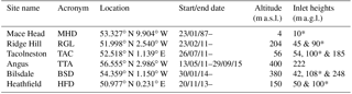
Table 2 Greenhouse gas and ozone-depleting substance species and instrumentation at each UK DECC site.

2.1 In situ measurements

We use tall-tower measurements and the atmospheric baseline observatory at MHD to provide a long-term in situ measurement record to underpin the main objectives of GAUGE. Tall towers (TTs) are used to collect atmospheric GHG measurements that are sensitive to fluxes on a horizontal scale of 10–100 s km. We also established a geographically dense network of observations to help isolate GHG emissions from individual sources.

Tall-tower measurement network

Figure 1 shows the geographical locations of the TTs that collect atmospheric measurements of GHGs (Tables 1 and 2) and provide the long-term, core measurement capability of the UK GHG measurement network. Sampling air high above the land surface reduces the influence of local signals that can compromise interpretation of observed variations of GHGs (Gerbig et al., 2003, 2009). With the exception of the MHD atmospheric research station (described below) air is typically sampled at least 50 m above the local terrain and at multiple heights (Table 1) to assess the role of atmospheric mixing in the planetary boundary layer.

Tables 1 and 2 describe the five TT locations and the MHD site used in the GAUGE project. High-frequency measurements of GHGs have been collected for the past 3 decades at the MHD Northern Hemisphere background measurement station on the west coast of Ireland. They predominately represent clean western baseline conditions for the UK and mainland Europe. These MHD data have been previously used to infer UK-wide GHG emissions (Manning et al., 2011). In 2012, the UK DECC tall-tower network was established across mainland UK using funding from the UK Department of Energy and Climate Change (with the responsibility now residing in the Department for Business, Energy and Industrial Strategy, BEIS). Three sites were established (Angus, Ridge Hill, and Tacolneston; Table 1) with the purpose of improving the spatial and temporal distribution of measurements across the UK to reduce uncertainties of GHG emissions for the devolved administrations (i.e. England, Wales, Scotland, and Northern Ireland). As part of the GAUGE project, we augmented the UK DECC network with two TT sites at Bilsdale and Heathfield (Fig. 1), which started collecting data from 2013 onwards. These two new sites were chosen to help fill the measurement coverage over mid-northern England, where there is significant industrial activity, and to collect measurements south of London. For detailed descriptions of each site, measurement and data logging instrumentation, and the calibration protocols we refer the reader to Appendix A; Stanley et al. (2017); and Stavert et al. (2018) – hereafter ARS18a.

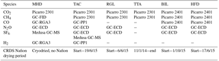
As an example, Fig. 2 shows CO₂, CH₄, and N₂O mole fraction data from Bilsdale, North Yorkshire. Figure 2 also shows the statistically determined baseline, long-term trend, and mean diurnal cycle for each season. The statistical fitting procedure is described in Thoning et al. (1989) and on the associated NOAA/ESRL website (http://www.esrl.noaa.gov/gmd/ccgg/mbl/crvfit/crvfit.html, last access: 8 August 2018). The mean Bilsdale growth rates for CO₂, CH₄, and N₂O are 3, 8, and 0.8 ppb yr⁻¹, respectively. The mean seasonal amplitudes for these gases are 18, 51, and 0.8 ppb, respectively. Table 3 summarizes the descriptive statistics for tall-tower data. Diurnal variations of the atmospheric mole fractions vary seasonally, particularly CO₂ and CH₄ that have large surface fluxes. Atmospheric mole fractions of CO₂, for instance, have a peak diurnal cycle of ≃10 ppm during summer months. Diurnal variations during winter months (≃3 ppm), particularly evident at lower inlet heights, provide some indication of the role of boundary layer height. Shallow wintertime boundary layer heights that are lower than an inlet height result in measurements of free-tropospheric air that is disconnected from direct surface exchange. Variations of CH₄ are due not only to changes in anthropogenic emissions but also to higher summertime OH concentrations, which represent the main loss term. N₂O has an atmospheric lifetime ≃120 years, determined by stratospheric photolysis. Our measurements show a growth rate that is consistent with the global value of ≃0.9 ppb yr⁻¹.

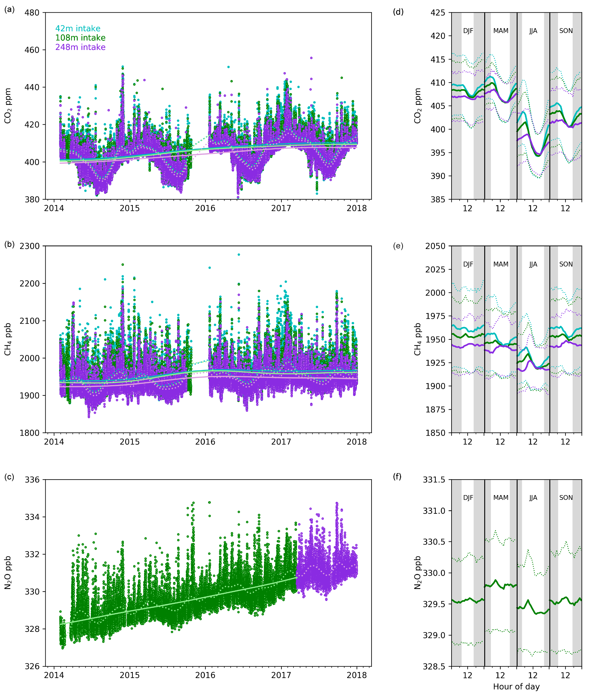
Figure 2 (a)–(c) Hourly mean of CO₂ (ppm), CH₄ (ppb), and N₂O (ppb) measurements at three inlet heights (42, 108, and 248 m) at Bilsdale, North Yorkshire, from March 2014 to July 2017 (Table 1). The statistical baseline (dashed line) and the long-term trend (solid line) are shown in the inset for each inlet height. (d)–(f) Mean seasonal diurnal cycle for CO₂, CH₄, and CO. The dotted lines denote the ±5th and 95th percentile. Statistical fitting procedures follow Thoning et al. (1989); further details can be found in ARS18a.

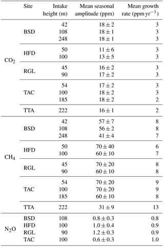
Table 3 Mean seasonal amplitude and mean growth rates of CO₂, CH₄, and N₂O at the Bilsdale (BSD), Heathfield (HFD), Ridge Hill (RGL), Tacolneston (TAC), and Angus (TTA) tall-tower sites. The mean seasonal amplitude (±1 standard deviation) was calculated from the annual peak-to-peak amplitudes. The mean growth rate is the average of the first derivative of the statistical long-term trend.

We also analysed the radiocarbon content of CO₂ (Δ¹⁴CO₂) at MHD and TAC as an approach to estimate the fossil fuel contribution to observed atmospheric variations of CO₂ (ffCO₂). The underlying idea is that fossil fuels, by virtue of their age, are devoid of ¹⁴C, which has a half-life of 5700±30 years (Roberts and Southon, 2007). Measurements of Δ¹⁴CO₂ have been used extensively to determine ffCO₂ (e.g. Meijer et al., 1996; Levin et al., 2003; Levin and Karstens, 2007; Turnbull et al., 2006, 2009; Graven et al., 2009; Berhanu et al., 2017). Our sampling strategy at MHD (nominally unpolluted site) and TAC (nominally polluted site) was designed to determine the west–east gradient of ffCO₂, reflecting the prevailing wind direction over the UK.

Weekly glass flask sample pairs were collected at MHD and TAC. A commercial sampling package is used at MHD (Sherpa 60, High Precision Devices Inc., USA) as part of the NOAA Global Greenhouse Gas Reference Network global flask sampling programme run by the Earth System Research Laboratory (ESRL). A similar system, custom-built by the University of Bristol, was used at TAC. Flask pairs have been filled at MHD for NOAA since 1991, but they have not been previously analysed for ¹⁴CO₂. We collected and additional flask from June 2014.

Weekly sampling commenced in June 2014 and concluded in February 2016. To determine the radiocarbon CO₂ content of our measurements, the samples are graphitized by the Institute of Arctic and Alpine Research (INSTAAR) and then sent for analysis to the accelerator mass spectrometer at the University of California at Irvine. Results are reported in Δ¹⁴C against the NBS oxalic acid I standard with an uncertainty of 1.8 ‰–2.5 ‰. Over the course of the GAUGE project a total of around 250 samples were analysed for ¹⁴CO₂. From this analysis we also received information about the stable isotopes ¹³CO₂, CO¹⁸O, and ¹³CH₄, which we do not report here. As part of the deployment of the Atmospheric Research Aircraft (ARA, described below) we collected glass flasks for the ¹⁴CO₂ and Tedlar bags for analysis of ¹³CH₄ by Royal Holloway, University of London. Using the aircraft allowed us to improve our knowledge of the spatial gradient of these gases. Samples were taken using an oxygen radical absorbance capacity (ORAC) metal bellows pump, fitted with a pressure relief valve. For the glass flask sampling an adapter containing a downstream pressure relief valve was used to prevent the accidental over-pressurizing of the glass flasks during flight sampling.

A preliminary study of ¹⁴CO₂ at Tacolneston during the GAUGE project has highlighted the benefits and difficulties associated with determining the fossil fuel content of CO₂ in the UK. The key outcome from the measurement programme has suggested that the amount of CO₂ originating from fossil fuel burning is not significantly different from model simulations using Emission Database for Global Atmospheric Research (EDGAR) emissions. However, there were a number of difficulties associated with making these measurements. First, we used a number of assumptions and data corrections to account for terrestrial biosphere fluxes and nuclear emissions. For nuclear emissions, we expect that the applied correction can be significantly improved by provision of higher-frequency emissions data from the nuclear industry. Second, the location of the sampling site, and timing and frequency of measurements are paramount in determining a strong enough ¹⁴CO₂ signal from fossil fuels to distinguish it from the background uncertainty. Many lessons were learnt in the GAUGE project that will allow for an improved and more robust sampling strategy to be applied to future measurements (Wenger et al., 2018).

East Anglian church network

A key objective of GAUGE was to improve understanding of how to attribute observed variations of GHGs to particular sectors. To help address that objective, we established a regional network of five sensors over East Anglia (Fig. 1, Table 4), where there is a high density of crop agriculture, a sector with large seasonal emissions of CH₄ and N₂O attributed to fertilizer application (Sect. 1). Developing this regional network supports the inference of higher-resolution emission estimates (Manning et al., 2011). We used data from this network to determine how well we can distinguish between sources of CH₄ that range from spatially diffuse agricultural sources to point sources such as landfills.

Table 4 Details of the measurements made in the GAUGE East Anglian network.

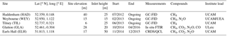
We purposely distributed the network across East Anglia (Fig. 1), comprising one atmospheric observatory (Weybourne) and three churches (Holy Trinity, Haddenham; All Saints, Tilney; and St Nicholas, Glatton), and one wind turbine (Earl's Hall). East Anglia is one of several dense regions of UK agriculture. It was chosen for two reasons: (1) there is little variation in terrain height, simplifying boundary layer transport and mixing, and (2) all sites are within an hour of Cambridge, simplifying logistics associated with maintaining long-term sites. Additional criteria for site selection included sufficient sampling height (15–50 m for the East Anglia network, Table 4), remoteness from very local sources of CH₄, easy accessibility for maintenance, and low running costs.

Figure 3 shows that the CH₄ mole fraction data collected from the three churches exhibit similar variations on diurnal, daily, and monthly timescales, suggesting that the surrounding villages have similar sources and/or at least some of the observed variation reflect larger-scale variations. Observed sub-annual variations of CH₄ at the Weybourne Atmospheric Observatory (WAO), for different years, are comparable to those at inland sites on seasonal timescales but are muted on faster timescales because it mainly observes clean upwind air. The shape of the diurnal cycle at the church sites suggests that the boundary layer height likely plays the dominant role. Seasonal variations reflect changes in regional sources, boundary layer variations, and the OH sink.

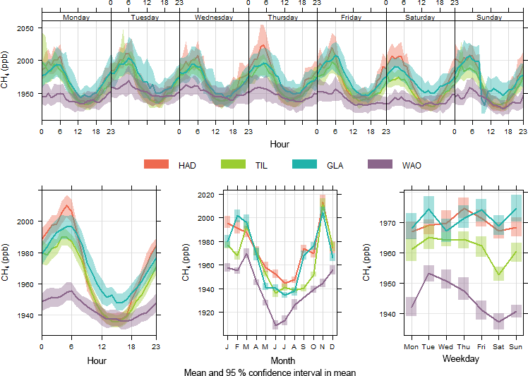
Figure 3 Observed variations of CH₄ mole fraction data collected at one atmospheric observatory (Weybourne, WAO, 13 February 2013–6 May 2014) and three church steeples at Haddenham (HAD, 3 July 2012–23 September 2015), Tilney (TIL, 7 June 2013–31 August 2015), and Glatton (GLA, 22 October 2014–5 April 2016). The coloured envelope denotes the 95 % confidence interval of the hourly, daily, and monthly mean.

Using the NAME-InTEM inverse model framework (Manning et al., 2011), we used the East Anglian network to infer county-level CH₄ fluxes for Cambridgeshire, Norfolk, and Suffolk. Our a posteriori fluxes were consistent with those from the UK National Atmospheric Emissions Inventory (Connors et al., 2018). For this work it was difficult to accurately estimate associated uncertainties because of difficulties associated with defining the “background” CH₄ entering into the small, regional domain chosen. This difficulty will be avoided when these data are included in larger, regional-scale inversions. We find that regional networks, embedded within a nationwide network, show great potential for revealing additional spatial and temporal details of emissions such as point source emissions from landfills (Riddick et al., 2017). Such a regional network would best serve a national-scale network over regions where a priori emission uncertainties are largest.

2.2 Mobile GHG measurement platforms

We use mobile platforms to help integrate measurements that are sensitive to different spatial scales. The two principal platforms we use are the Rosyth–Zeebrugge North Sea ferry and the British Aerospace 146 (BAe-146) Atmospheric Research Aircraft. We also describe the deployment of balloon-borne sensors and a fixed-wing UAV, as examples of GAUGE fostering new atmospheric GHG measurement technology. In the conventional sense, a mobile measurement platform is one that is fixed in one place for some length of time but is sufficiently mobile that it can be moved elsewhere to continue measurements. The ferry platform can be considered a continually moving mobile platform.

2.2.1 North Sea ferry

We installed an 8 ft. air-conditioned sea container on the Rosyth (56.02262^∘ N, 3.43913^∘ W)-to-Zeebrugge (51.35454^∘ N, 3.175863^∘ E) ferry operated by DFDS Seaways. The container includes a Picarro 1301 cavity ring-down spectrometer (CRDS) to measure mole fractions of CH₄, CO₂, and H₂O. This ship of opportunity completes three return journeys per week, traversing the North Sea at different times of day, thereby minimizing temporal measurement bias, which can sometimes complicate the analysis of data from mobile platforms. The prevailing winds over the North Sea are westerly and southwesterly, so that measurements frequently sample the outflow from the UK, and also allow us to distinguish between UK and mainland European emissions.

Figure 4 shows the view from the mobile laboratory, with sample inlets located at the bow away from local sources on the ferry (chimney stacks towards the stern). The initial installation was on 25 February 2014 on DFDS Seaways Longstone (now the Finnmerchant) and ran until 15 April 2014. A weather station (Vaisala WXT 520) located on the top deck provides basic meteorological data (air temperature, pressure, wind speed and direction); geolocation information (latitude, longitude, ship speed, course) is obtained from a Garmin GPS unit fixed to the roof of the sea container.

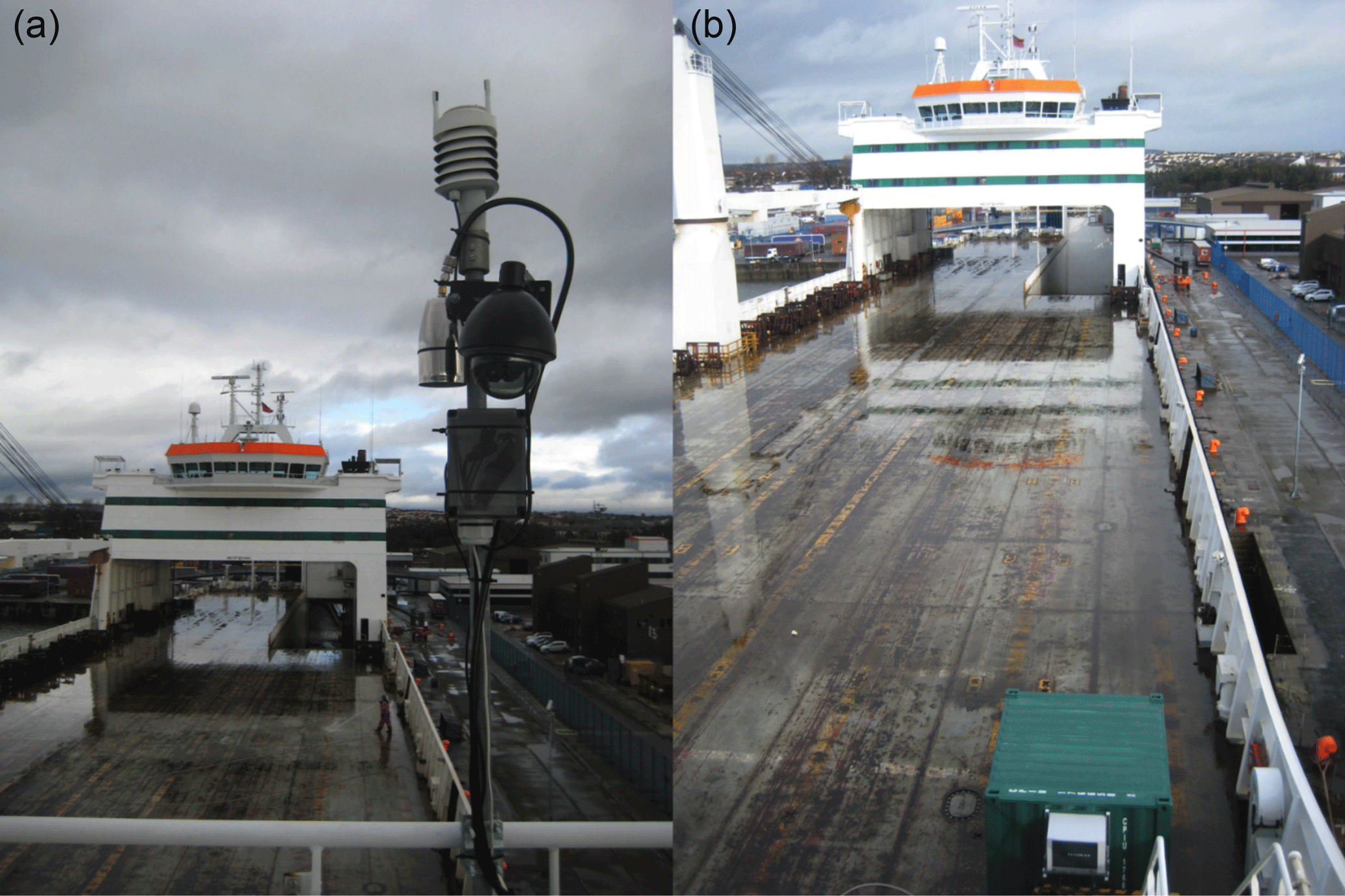
Figure 4 Photos of the North Sea ferry mobile GHG laboratory on the DFDS Seaways Longstone (now the Finnmerchant). View of the (a) weather station mounted on the top deck and (b) from the air inlet mounted on top of the mobile laboratory located on the weather deck.

Figure 5 shows example CH₄ data for sailings in March, April, July, and September 2014, which shows a dynamic range that reflects geographical variations in sources. Differences between individual sailings reflect changes in seasonal emissions and prevailing meteorology. Figure 5 shows instances when observed values are influenced by emissions from the UK and the North Atlantic background during spring and summer (Fig. 5a, b), and when observed values are influenced by high emissions from Germany and central Europe (Fig. 5c) and by lower emissions from Scandinavia (Fig. 5d). To avoid contamination from GHG emissions on board the ship (e.g. engine emissions, venting of the below-deck cargo area), individual data points were removed when the ship was in port or when the wind blew from the direction of the chimney stacks. A more detailed description of the instruments and the data interpretation can be found in Helfter et al. (2018).

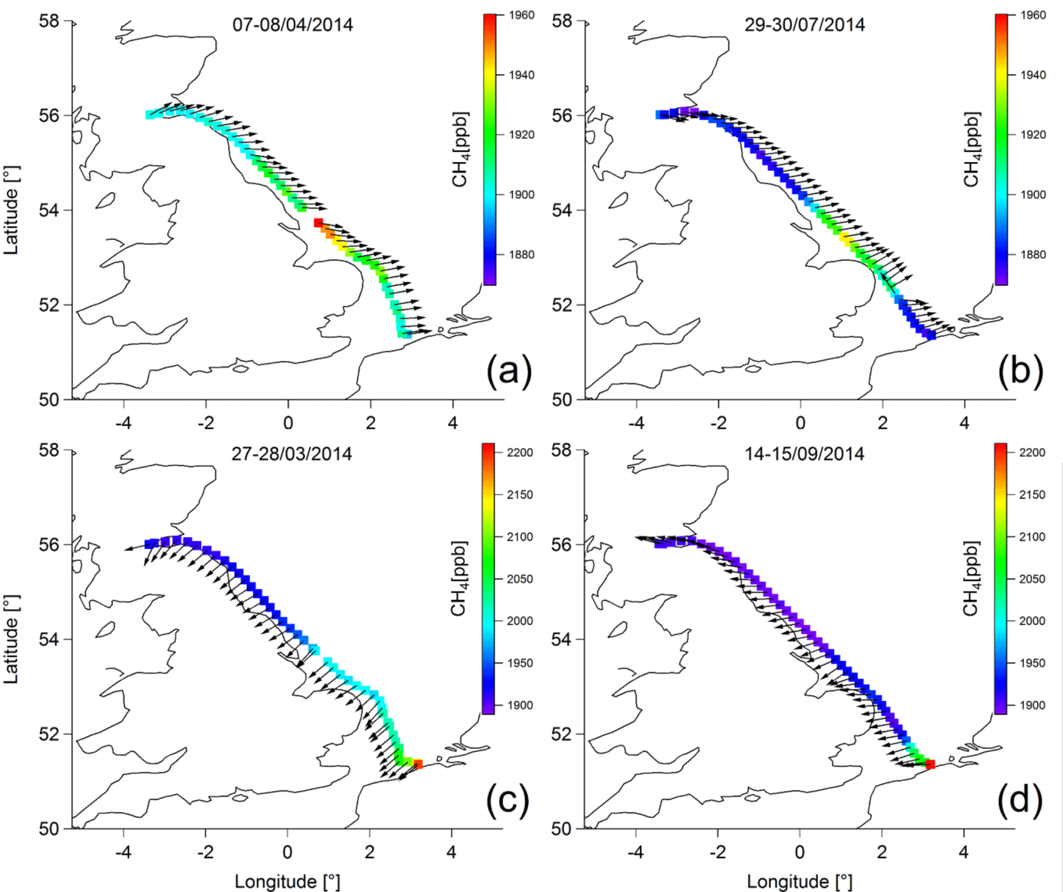
Figure 5 Observed temporal and spatial variations in CH₄ mole fractions along the route of the DFDS freight ferry in March, April, July, and August 2014. Arrows denote local wind direction.

2.2.2 BAe-146 Atmospheric Research Aircraft

We use the NERC/Met Office Atmospheric Research Aircraft (ARA), operated by AirTask Group Ltd, to provide vertical profile distributions of atmospheric GHGs over and around the British Isles. The specific objectives of deploying the ARA include (1) collecting a snapshot of precise and traceable GHG concentration distributions over and around the UK; (2) integrating atmospheric GHG information collected by tall towers, ferry transects, and space-borne instruments; (3) defining and executing sampling experiments to enable measurement-led quantification of GHG fluxes at the regional scale (𝒪(100 km)); and (4) defining and executing sampling experiments to challenge Earth system models and inversion models in terms of better understanding model atmospheric transport error and surface emission distribution.

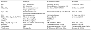
The ARA is a BAe-146-301 aircraft that has been converted to a mobile laboratory, including a variety of forward- and backward-facing external inlets so that air can be sampled by instruments within the main cabin. It also includes a number of ports that can host remote-sensing instruments. Table 5 describes the instruments that we deployed during GAUGE, including in particular instruments that measure CO₂, CH₄, and N₂O, and a small complementary suite of other trace gases and thermodynamic parameters. We made continuous measurements of CO₂ and CH₄ at a frequency of 1 Hz using a Fast Greenhouse Gas Analyzer (FGGA, Los Gatos, USA). For a detailed description of the FGGA – including its operating principles, data processing, and calibration – we refer the reader to O'Shea et al. (2013). We also collect 1 Hz measurements of N₂O and CH₄ from a quantum cascade laser absorption spectrometer (Aerodyne Research Inc., USA). Further details of the instrument are described by Pitt et al. (2016). We use the Met Office Airborne Research Interferometer Evaluation System (ARIES), a Fourier transform infrared spectrometer (FTIR), to retrieve partial columns of CH₄ and CO₂ and vertical profiles of H₂O and temperature. Further details about ARIES can be found in Allen et al. (2014). Other instruments listed in Table 5 are core ARA science instruments, which are described in Allen et al. (2011) and references therein.

Gerbig et al. (1999)O'Shea et al. (2013)Pitt et al. (2016)Di Carlo et al. (2013)Lewis et al. (2013)Allen et al. (2014)Ström et al. (1994)Petersen and Renfrew (2009)Brown et al. (1983)

Table 5 Key instrumentation on board the FAAM aircraft for GAUGE-specific flights, including measurement principles and references to instrument characteristics (where available). VUV denotes vacuum ultraviolet (light); HFCs, PFCs, and VOCs denote hydrofluorocarbon, perfluorocarbons, and volatile organic compounds, respectively; and PRT denotes platinum resistance thermometer.

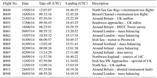
During GAUGE we conducted a total of 16 individual flight sorties over/around mainland UK and Ireland between May 2014 and March 2016, comprising over 65 h of atmospheric sampling. These flights are summarized in Table 6 and Fig. 6. A typical flight sortie coordinated upwind and downwind sampling of a target flux region (e.g. the London metropolitan area), based on the prevailing boundary layer wind direction, to attempt sampling of air masses that have been impacted by regions with GHG emissions and uptake. We also designed flights to sample outflow from mainland UK and continental Europe, and outflow from the Irish and North seas on days with strong westerly flow regimes (e.g. Pitt et al., 2018).

To capture regional emissions during GAUGE, we collected measurements that were mostly in the boundary layer, as defined by in-flight thermodynamic profiling, which was typically below 2 km altitude. Occasionally, to characterize long-range transport of pollutants into our study region, we collected measurements during deeper vertical profiles into the free and upper troposphere. Other flight profiles included surveys around Britain and Ireland and flying around tall towers, as described below.

Figure 6 shows a summary plot of the CO₂ and CH₄ data collected during GAUGE. In particular, it illustrates the horizontal and vertical spatial coverage of the aircraft sampling and the dynamic range of mole fractions sampled. These observed variations are due to differences in flight altitude and the time of year of the superimposed flights (Table 6), differences in air mass history, and the spatial and temporal variability of local and regional fluxes across seasons and sources.

2.2.3 Balloon CO₂ sondes

Balloons offer an alternative platform for the collection of vertical profiles of GHGs, building on the approaches used widely by the meteorological and stratospheric communities. Here, we describe some of the first balloon launches of small-scale CO₂ sensor technology that have been adapted for atmospheric sciences as part of a collaboration between the University of Cambridge, SenseAir (Sweden, https://senseair.com/, last access: 8 August 2018), and Vaisala (Finland). The instrument consists of a small, sensitive nondispersive infrared (NDIR) CO₂ sensor developed by SenseAir. The instrument sampling is 1 Hz with data transmitted to the Vaisala MW41 ground station via a Vaisala RS41 radiosonde. The corresponding vertical resolution of the collected data is 4–5 m. The dimensions and weight of the instrument package are approximately $\mathrm{150}\times \mathrm{150}\times \mathrm{300}$ mm and 1 kg, respectively. Heavy-duty cable ties are used to seal the enclosure and secure the radiosonde to the outside. A 1200 g balloon (TOTEX, Japan) is used for lifting the payload up to a ceiling of ≃35 km. A typical flight is 3–4 h, including rapid descent of 20–30 mins. The system used during GAUGE is expendable but could be easily recycled with the installation of an onboard GPS sensor.

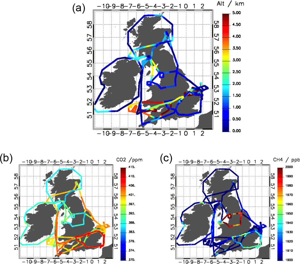
Figure 6 Flight tracks for all FAAM flights during GAUGE from 15 May 2014 to 4 April 2016 (Table 6). Colours denote (a) altitude, (b) CO₂ mole fraction, and (c) CH₄ mole fraction.

Figure 7 shows preliminary data from two ChemSonde launches from WAO on 14 April 2016 to test the viability of the system. Met Office surface analysis charts (not shown) indicate that the UK was under the influence of a low-pressure anticyclone in the North Atlantic, transporting moist air over the southern half of the UK, during the period of measurements. A low-level stratus cloud deck, with drizzle, and low SW winds predominated over WAO during the morning of 14 April, with light winds and steady rain during the afternoon. The first instrument was launched at 10:39 UTC, and the second at 14:30 UTC. For brevity, we only show data to 10 km. The sharp decrease in CO₂ from near-surface altitudes to ≃1 km during the morning launch and the increase in boundary layer CO₂ concentrations from morning to afternoon launches suggest some local influence. We also noticed that some small-scale increases in CO₂ (1.8 and 7.5 km from the morning launch and 2.5 km from the afternoon launch) correspond to increased relativity humidity, indicating possible cloud layers. NOAA HYSPLIT 48 h back trajectories (Stein et al., 2015) initialized at these lower and mid-troposphere altitudes (not shown) indicate that we are sampling background maritime air over the North Atlantic that has been lofted prior to interaction with land surfaces. Differences in relative humidity close to 6 km suggest that the morning cloud structure has been dissipated by the stronger afternoon winds. We attribute the 4–5 ppm difference between CO₂ instruments above 6.5 km to problems with the zero baseline drift and to a faulty span measurement during the afternoon pre-launch preparation. Further studies with ChemSonde are planned, with emphasis on improving design, operation, and post-processing of data.

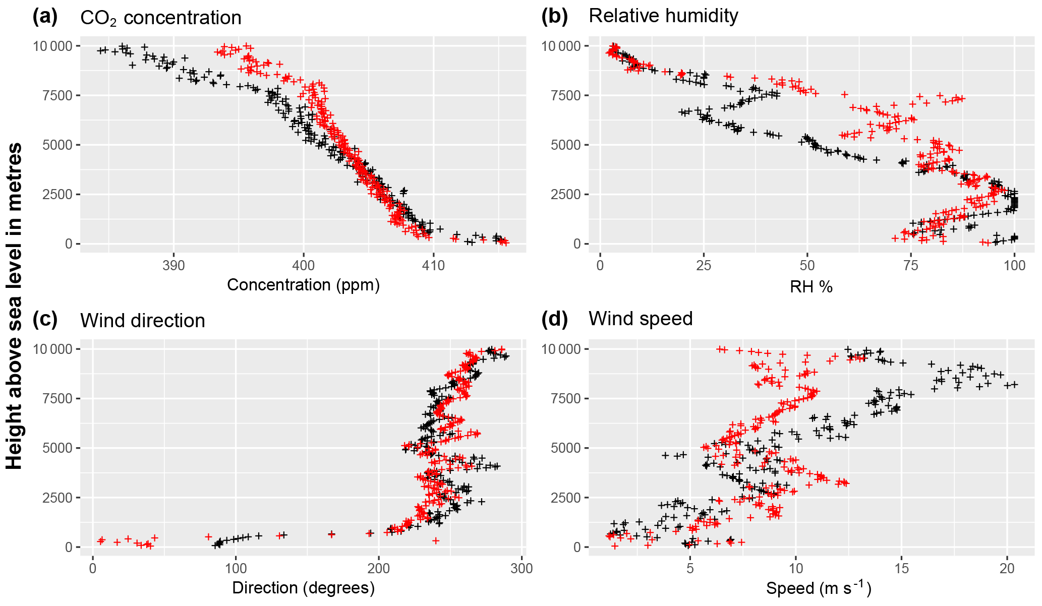
Figure 7 Preliminary balloon-borne CO₂ data launched on 14 April 2016 from Weybourne Atmospheric Observatory, UK (Fig. 1). Correlative measurements of (b) relative humidity, (c) wind speed, and (d) wind direction are also shown. Data are averaged every 10 s. Red ticks denote the morning launch, and black ticks denote the afternoon launch.

2.2.4 Unmanned aerial vehicles for hotspot measurement campaign

UAVs represent a new atmospheric measurement platform for studying atmospheric GHGs. They can be deployed rapidly to provide vertical information across a horizonal dimension 𝒪(100 m). Within GAUGE, researchers used a variety of measurement technologies, including fixed-wing and rotary UAVs, to develop and refine new methods to use atmospheric measurements to quantify CH₄ and CO₂ emission from a landfill site (Riddick et al., 2016, 2017; Sonderfeld et al., 2017; Allen et al., 2018a). This represents one of the first demonstrations of using UAVs to sample GHG emissions. The reader is referred to Allen (2014) and Allen et al. (2015) for further details of the underlying technology.

We conducted a 2-week measurement campaign at a landfill site near Ipswich, England (operated by Viridor Ltd), in August 2014. This campaign brought together researchers from the University of Bristol, University of Cambridge, Denmark Technical University, University of Edinburgh, University of Leicester, University of Manchester, Royal Holloway University of London, University of Southampton, and Ground Gas Solutions (GGS) Ltd. The landfill includes historic, capped and active, and open landfill cells; a leachate plant; a gas collection network; and a gas-burning energy generation facility.

We equipped the site with a 20 m eddy covariance flux tower, three Los Gatos Research Ultraportable Greenhouse Gas (CO₂ and CH₄) Analyzers (triangulated across the capped and open cell areas), a closed-path FTIR, and five 3-D sonic anemometers to characterize flow over the site. Conventional walkover flux surveys were conducted by GGS, and dynamic automated flux chambers were operated on the flanks of the capped landfill area to investigate seeps under the capped area where this met an active cell. Tracer releases of perfluorocarbon and acetylene were also conducted from various key points across the site to allow proxy flux calculations from mobile (public road) plume sampling downwind. Specific experiments and instrument siting were designed on each day of the intensive period in response to weather (especially wind) conditions to characterize inflow and outflow from different areas of the site. We deployed a fixed-wing UAV equipped with a CO₂ NDIR sensor around the site (Edinburgh Instruments Gascard NG). We also launched a tethered rotary UAV, which sampled air up to 120 m above the local terrain. This air was analysed using a ground-based instrument (Los Gatos Research Ultraportable Greenhouse Gas Analyzer) via a 150 m length of Teflon tube. This configuration allowed us to sample vertical profiles of CH₄ and CO₂ over the landfill site.

We also established a fixed-site monitoring station measuring CO₂ and CH₄ mole fractions to put the campaign into a longer temporal context, to help test plume inversion techniques, and to test the efficacy of continuous in situ monitoring to generate flux climatologies (Riddick et al., 2016, 2017). Sonderfeld et al. (2017) demonstrate how to combine a computational fluid dynamics model (which accounts for topographical data from a 3-D lidar survey data) with continuous in situ FTIR measurements to infer and apportion fluxes across the surface area of the landfill site. They showed in particular the ability of this approach to distinguish between individual emission regions within a landfill site, allowing better source apportionment compared with other methods that derive bulk emissions.

Our UAV deployment during this experiment has since led to further refinements to the method and platform, and to our use of similar technology to infer fluxes from other UK landfills (Allen et al., 2018a). A recent validation of a new mass balancing algorithm based on tethered UAV sampling of a known CH₄ release rate demonstrated that a 20 min flight on a single rotary UAV flight can reproduce the known release rate with an mean accuracy of 14 % and an (1σ) uncertainty of <40 % (Allen et al., 2018b). Collectively, these measurements allowed us to test and compare a wide range of established and novel sampling technologies and flux quantification approaches. It also allowed us to examine how to optimize different combinations of data to determine net bulk (whole-site) GHG fluxes.

2.3 Space-borne observations of GHGs

Satellites provide global, near-continuous, and multi-year measurements of GHGs that are used to infer GHG fluxes on sub-continental scales and to provide boundary conditions for regional atmospheric transport models. Within GAUGE, we explore the potential of short-wave infrared (SWIR) column measurements of CO₂ and CH₄ from the Japanese Greenhouse Gases Observing SATellite (GOSAT) and thermal IR column measurements of CH₄ from the European Infrared Atmospheric Sounding Interferometer (IASI). For the sake of brevity, we describe here only the pertinent details of GOSAT and IASI and refer the reader to other studies dedicated to these satellite instruments (e.g. Kuze et al., 2009; Clerbaux et al., 2009).

GOSAT is the first space-borne mission dedicated to measuring GHGs. It was launched in a sun-synchronous orbit with a local overpass time of 13:00 by the Japanese Space Agency (JAXA) in January 2009 (Kuze et al., 2009). We use the Thermal And Near-infrared Sensor for carbon Observation (TANSO) Fourier transform spectrometer (FTS), which observes atmospheric spectra, and the Cloud and Aerosol Imager (CAI), which provides multi-spectral imagery and coincident cloud and aerosol information (Kuze et al., 2009). TANSO-FTS has a ground footprint of approximately 10.5 km² and returns to the same point every 3 days. For illustration, we show GOSAT SWIR dry-air column-averaged CH₄ mole fractions that are inferred from version 7.0 of the proxy retrieval developed by the University of Leicester (Sect. 3). These data are sensitive to changes in atmospheric CH₄ in the lower troposphere. The proxy retrieval method simultaneously fits CH₄ and CO₂ spectral features in nearby wavelengths. The underlying idea is that taking the ratio of the CH₄ and CO₂ fitted in nearby wavelength regions effectively removes spectral artefacts common to both CH₄ and CO₂ (e.g. scattering). The conventional method of using these data is to multiply the ratio by model CO₂, assuming that CO₂ varies in space and time less than CH₄. The resulting proxy XCH₄ data have been evaluated extensively using data from the Total Carbon Observing Network (Parker et al., 2011, 2015).

Table 6 Diary of FAAM survey flights for GAUGE between May 2015 and March 2016, including take-off and landing times, sampling locations, and a brief description of mission profiles.

IASI is one of a series of FTS instruments on the polar-orbiting meteorological MetOp platforms (Hilton et al., 2012) designed primarily for operational meteorology. There are two IASI instruments currently operating: MetOp-A was launched on 19 October 2006, and MetOp-B was launched on 17 September 2012. IASI has an across-track measurement swath of 2200 km, resulting in near-global coverage twice a day with a local solar overpass time of 09:30 and 21:30. It measures three spectral bands that span a range of thermal IR wavelengths from 4 to 15.5 µm (Clerbaux et al., 2009), which are most sensitive to CH₄ in the mid-troposphere. Vertical profile retrievals of column-averaged volume mixing ratios of atmospheric CH₄ have been inferred using optimal estimation from IASI spectra by the Rutherford Appleton Laboratory (Siddans et al., 2017). The retrieval produces two pieces of information in the mid- and upper troposphere each with a single retrieval precision of 20–40 ppbv. Differences between IASI and GOSAT CH₄ are within 10 ppbv except over southern mid-latitudes, where IASI is lower than GOSAT by 20–40 ppbv (Siddans et al., 2017).

The spatial coverage of satellite SWIR observations of CO₂ and CH₄ over the UK is limited mainly by cloud-free scenes that are themselves determined by the spatial resolution of the instruments and the repeat frequency of the orbits. Currently, there are insufficient cloud-free data to overtake the information provided by the in situ measurements. However, we will soon have daily CH₄ measurements from TROPOMI aboard Sentinel-5P, launched 16 October 2017. Data from future and planned missions represent at least an order of magnitude more satellite data than we have now. Until then, these GOSAT data represent constraints on larger-scale sub-continental CO₂ and CH₄ flux estimates (e.g. Feng et al., 2017).

2.4 Calibration activities

Linking measurements in the GAUGE network to a common calibration scale ensures comparability of these measurements, and simultaneously linking them to a common set of traceable gas standards ensures they are also compatible with ongoing international GHG measurement activities. Prominent examples of such activities include the NOAA/ESRL GHG reference network, ICOS, and IG³IS (https://goo.gl/4t1x6i). This approach also minimizes any associated systematic errors for flux estimation using Bayesian inference methods.

The GAUGE project encompassed a large number of data streams collected using a range of instrumental techniques and at a variety of temporal resolutions, increasing the risk of compatibility and comparability errors. Inversion methods used in GAUGE to infer GHG fluxes from atmospheric mole fraction measurements are particularly sensitive to site biases and offsets (Law et al., 2008). Consequently, ensuring comparability and assessing compatibility were key to the success of GAUGE.

As far as possible we ensured measurement comparability by linking all observations directly to common World Meteorological Organization (WMO) calibration scales, but due to the historical nature of some data records this was not uniformly possible. All CO₂ measurements collected within the project were linked to the WMO x2007 scale. All CH₄ measurements other than MHD gas chromatography–flame ionization detector (GC-FID; Table 2), which uses the Tohoku scale, were calibrated to the WMO x2004A scale. In contrast, N₂O measurements used either the Scripps Institute of Oceanography 1998 (SIO-98) scale (MHD and the rural tall-tower sites BSD, HFD, RGL, TAC, and TTA) or the WMO x2006A scale (all other locations).

3 Numerical models of atmospheric GHGs

Figure 8 shows the modelling strategy we employed to quantify the magnitude, distribution, and uncertainty of UK emissions of GHGs. We use models of atmospheric chemistry and transport, using prescribed a priori flux estimates, to describe the relationship between sector emissions of GHGs and atmospheric variations observed by the fixed and mobile GHG measurement platforms used during GAUGE (Fig. 1). These models, which account for instrument-specific sampling, constitute the forward model. Inverse models infer the magnitude and uncertainty of regional flux estimates by fitting the forward model to observations, accounting for their respective uncertainties.

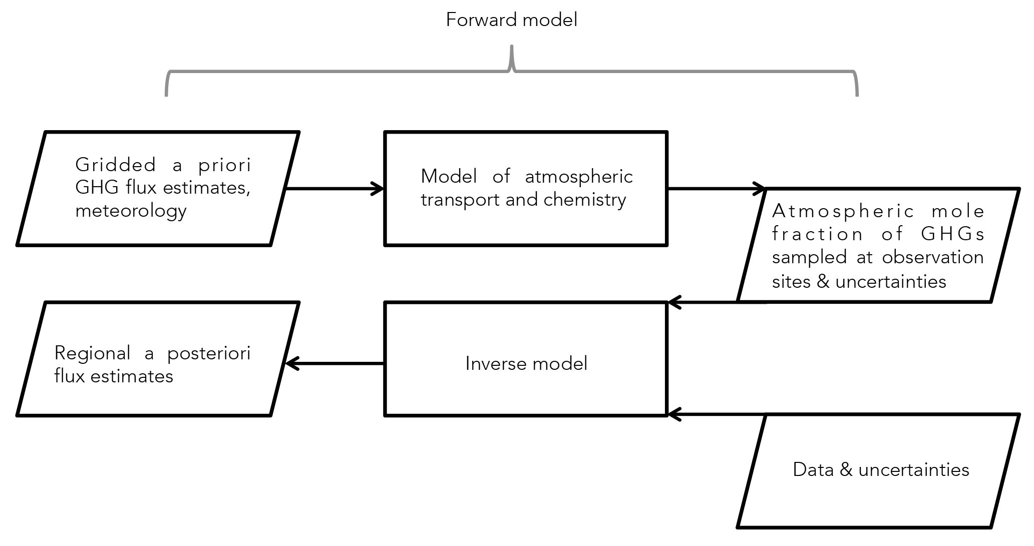
Figure 8 Schematic of the generalized GAUGE modelling strategy. The diagram neglects the non-linear inverse modelling approaches.

Because of the complex physical and chemical relationships between the surface fluxes and the atmospheric observations, and because of the assumptions embedded within individual models, we use a range of atmospheric transport models and inverse methods to quantify the role of model transport error on a posteriori fluxes.

3.1 Atmospheric chemistry transport models

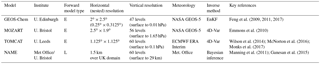
Table 7 summarizes the three different chemical transport models (CTMs) and one atmospheric dispersion model that we use to interpret the GAUGE data. All models are well established and have been used to interpret a wide range of atmospheric GHG measurements.

3.2 Brief description of individual models

We use the following models: (1) the Goddard Earth Observing System atmospheric Chemistry transport model (GEOS-Chem) (Feng et al., 2011, 2017; Fraser et al., 2013; Deng et al., 2014); (2) the Model for OZone and Related chemical Tracers (MOZART) (Emmons et al., 2010); (3) the TOMCAT model (Wilson et al., 2016; McNorton et al., 2016; Monks et al., 2017); and (4) NAME (Jones et al., 2007). These models vary in their basic methodologies for representing atmospheric transport, parameterizations of physical atmospheric processes, and horizontal and vertical resolutions. GEOS-Chem, MOZART, and TOMCAT are global Eulerian models, and NAME is a Lagrangian dispersion model that is applied on a regional basis. We also use GEOS-Chem in a nested model that involves running it at a higher resolution over a limited geographical domain with boundary conditions determined by a coarser global simulation with consistent flux inventories. The boundary conditions for NAME are solved as part of the inverse problem. Model differences therefore provide us an opportunity to quantify the impact of model error on describing observations and consequently on inferred GHG flux estimates. For further details about an individual model, the reader is encouraged to consult the model-specific literature as provided above.

For the purpose of this overview of GAUGE and as part of our model assessment within GAUGE, we ran global 3-D experiments to describe observed variations of CO₂, CH₄, and N₂O from 2004 to 2016, including the main GAUGE measurement period of 2014–2015, inclusively. The CTMs used common flux estimates and chemical loss fields as described below. Preparation of these estimates, collected from different sources, were regridded to the different model resolutions (Table 7), ensuring that the total emitted mass was conserved. The CTMs also used common atmospheric mole fraction initial conditions for 2003.

To describe anthropogenic emissions of CO₂ from 2003 to 2009, we use the Carbon Dioxide Information Analysis Center (CDIAC) inventory (available online at http://cdiac.ornl.gov/trends/emis/overview.html, last access: 8 August 2018). In later years, we repeat values from 2009. We use the NASA-CASA biosphere model (Olsen and Randerson, 2004) to describe terrestrial biospheric fluxes during 2003–2015, including biomass burning emissions. Climatological ocean fluxes of CO₂ are taken from Takahashi et al. (2009), covering the period 2003–2011. We acknowledge that there are errors associated with using climatological flux estimates. However, the purpose of this model intercomparison was to assess the model spread associated with simulating atmospheric CO₂, CH₄, and N₂O.

The formulation of our CH₄ simulations generally follows Wilson et al. (2016) and McNorton et al. (2016). We use updated anthropogenic CH₄ emissions from the EDGAR v4.2FT inventory (Olivier et al., 2012), covering the period 2000–2010. We repeat 2010 emissions for years beyond 2010. Biomass burning emissions were taken from the Global Fire Emissions Database (GFED) v3.1 inventory (van der Werf et al., 2010). Wetland and rice emissions were taken from Bloom et al. (2012). Other natural emissions, including the soil sink (treated as a negative flux), were taken from the TransCom CH₄ model intercomparison (Patra et al., 2011). We use monthly 3-D mean OH fields taken from Patra et al. (2011) to describe the main atmospheric sink of CH₄. Reaction rates are taken from Sander et al. (2006). Stratospheric loss of CH₄ due to reaction with O(¹D) and Cl radicals are based on loss rates taken from the Cambridge 2-D model (Velders, 1995). The resulting atmospheric lifetime of CH₄ is ≃10 years, which is determined mainly by the tropospheric OH sink.

Fluxes for our N₂O simulations are taken from four broadly defined source categories: natural soils (Saikawa et al., 2014), agricultural and other anthropogenic emissions (Olivier et al., 2012), ocean fluxes (Manizza et al., 2012), and biomass burning (van der Werf et al., 2010). We parameterized an offline stratospheric loss of N₂O in each model using photolysis and O(¹D) climatologies (Thompson et al., 2014). We did not consider this sink for NAME because of the short duration of model runs compared to the atmospheric lifetime of N₂O (≃120 years). The relatively long atmospheric lifetime of N₂O, determined by stratospheric sinks, means that interpreting observed tropospheric variations of N₂O presents different challenges to interpreting observed variations of CH₄.

Feng et al. (2009, 2011, 2017)Emmons et al. (2010)Wilson et al. (2014); McNorton et al. (2016)Monks et al. (2017)Manning et al. (2011); Ganesan et al. (2015)

Table 7 Model descriptions used in the GAUGE intercomparison. Forward model types include Eulerian (E) and Lagrangian (L).

3.3 Assessment of model performance using large-scale independent data

To assess the global-scale GAUGE models, we use data that are representative of large spatial and temporal scales. In particular, we use surface mole fraction data from NOAA/ESRL and column data from the GOSAT and IASI satellite instruments (Sect. 2). We use these data to evaluate the three CTMs, described above, by sampling each model at the time and location of each observation.

Figure 9 shows that the models reproduce the broad-scale zonal-mean distribution of CO₂ and CH₄. Given the common set of source and sink terms, model divergence will mostly reflect differences in atmospheric transport. The latitudinal distribution has been normalized to the South Pole value for each model to account for the drift (incorrect sources/sinks) associated with the 8-year simulation. Generally, the largest model biases for CO₂ are at mid- and high northern latitudes, where the emissions are largest, but will also be reflected in interhemispheric transport times. Model divergence is highest at these latitudes during northern winter months, with GEOS-Chem having the largest model bias during these months. Model performance generally improves in the northern summer months, with model differences typically within a few ppm and much closer to the observations. The outlier (≃23 ppm) at 44^∘ N is the Black Sea site in Constanţa, Romania, which we believe is influenced by local emissions that are not included in our models. The model spread supports our strategy of using different models to infer GHG fluxes. For CH₄, the models have a similar level of skill. None of the models reproduce the observed interhemispheric gradients, likely due to errors in the a priori distribution of emissions used by the inventories. The model spread is largest in January with a value of 45 ppb. Model performance for N₂O is the most variable, although this partly reflects that N₂O has the smallest observed interhemispheric gradients of the three gases. The maximum model range is 1.4 and 1.7 ppb in January and July, respectively. The GEOS-Chem and MOZART models have gradients similarly small in the Southern Hemisphere and tropics, while TOMCAT is much larger. We find this model spread plays only a small role in our UK-centric inversion because of the higher density of data available over that region.

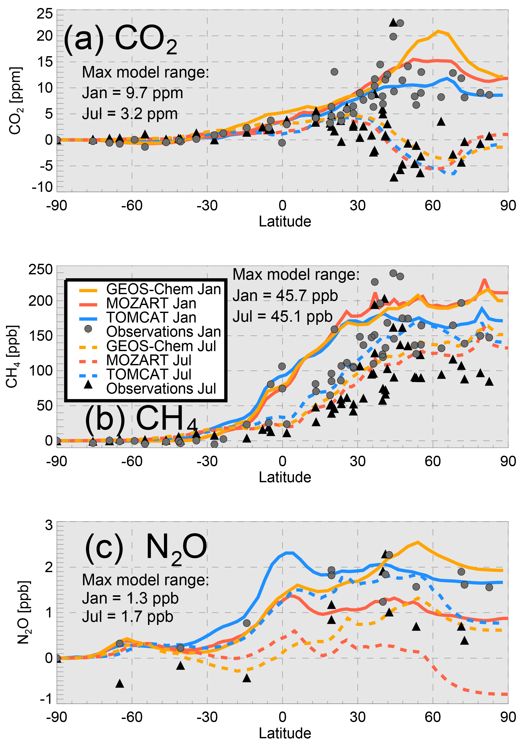
Figure 9 Simulated and observed surface zonal-mean latitudinal gradient of (a) CO₂ (ppm), (b) CH₄ (ppb), and (c) N₂O (ppb) in January (solid lines and circles) and July (dashed lines and triangles) 2011. Observations are made as part of the NOAA/ESRL measurement campaign. For each model, its South Pole value is subtracted for all latitudes. Observations are treated similarly.

Figure 10 shows an example comparison between the GEOS-Chem, TOMCAT, and NAME models and the observed atmospheric CO₂ mole fraction at the Bilsdale tall-tower site (Fig. 2). GEOS-Chem and TOMCAT models use CO₂ fluxes that have been pre-fitted to global-scale NOAA/ESRL data, while the NAME model uses atmospheric mole fraction boundary conditions taken from the MOZART model that have been adjusted downwards by 20 ppm to match NOAA data. The seasonal cycle represents the largest observed mode of variability, which the models capture with Pearson correlations r²>0.7 (range: 0.7–0.8). The annual mean model minus observation difference ranges from −0.3 to 1.7 ppm. These differences are greatly reduced after the models have been fitted to GAUGE tall-tower data (not shown).

Figure 11 shows that MOZART and GEOS-Chem have similar vertical distributions of CH₄ during January, displaying a stronger vertical gradient from the surface to 400 hPa than the TOMCAT model. This corresponds to higher northern hemispheric mole fraction values. During July, the three models all display different rates of vertical transport throughout the Northern Hemisphere troposphere. TOMCAT has a slight gradient between the surface and 600 hPa, and a much steeper gradient above; MOZART displays the opposite behaviour; and GEOS-Chem lies between those extremes. Differences in atmospheric transport are important and for some gases can represent a substantial fraction of the signal. Our use of multiple models and combining the resulting analysis improves our ability to quantify the uncertainty of our results.

We also evaluate the models using the GOSAT proxy XCH₄ V7.0 data product developed by the University of Leicester (http://www.esa-ghg-cci.org/, last access: 8 August 2018) and the IASI MetOp-A thermal IR V1.0 XCH₄ data products developed by the Rutherford Appleton Laboratory (http://dx.doi.org/10.5285/B6A84C73-89F3-48EC-AEE3-592FEF634E9B, last access: 8 August 2018).

Figure 10 Observed and model atmospheric CO₂ mole fraction values at the Bilsdale tall tower during 2014 (Fig. 2 and Table 1). All models are sampled at the latitude and longitude and the 250 m inlet altitude of the Bilsdale site.

Figure 12 shows the spatial coverage provided by both instruments during June–August 2014. The sparser coverage of GOSAT observations reflects its sensitivity to clouds and aerosols. Measurements over the ocean used a glint observing model that takes advantage of specular reflection and its associated high signal-to-noise ratio. Despite GOSAT and IASI observing different parts of the atmosphere, there are many common features associated with fossil fuel extraction/combustion (North America, China, and parts of Saudi Arabia), wetlands (South America, Africa, and part of India and China), and rice paddies (mostly India and China). Both GEOS-Chem and TOMCAT models reproduce the broad spatial distributions of GOSAT and IASI CH₄ observations (not shown), with negative global mean model biases that are approximately 10 ppb for GOSAT and between 1 ppb (GEOS-Chem) and 10 ppb (TOMCAT) for IASI.

3.4 Inverse methods

The ultimate objective of GAUGE is to characterize the magnitude, distribution, and uncertainty of UK GHG emissions. Relating a priori GHG flux estimates to the atmosphere sampled at the time and location of observations is called the forward problem (Fig. 8). The corresponding inverse problem refers to the process of relating observed atmospheric measurements to the underlying geographical distribution of GHG fluxes. Each of the atmospheric transport models listed above employs its own inverse method, as described below. Individual inverse methods employed in GAUGE have generally used all data described in Sect. 2, either as constraints for flux estimates or as independent data for model evaluation of a posteriori fluxes. Different assumptions employed by these inverse methods, e.g. description of atmospheric model transport error and specification of error covariances, will also contribute to the spread of a posteriori flux estimates.

Inferring CO₂, CH₄, and N₂O fluxes directly from atmospheric observations is generally an ill-posed inverse problem, with a wide range of scenarios that could fit these data. A priori information is used to regularize the problem (Fig. 8).

The results of inverse modelling are typically dependent on the distribution of the observations used. For example, the sparsity of data at low latitudes places a limit on our ability to infer GHG fluxes over geographical regions that are not well sampled, e.g. tropical ecosystems. The spatial and temporal density of GHG measurements collected during GAUGE allows us to constrain a posteriori emission estimates on a devolved UK administration scale and on sub-annual timescales.

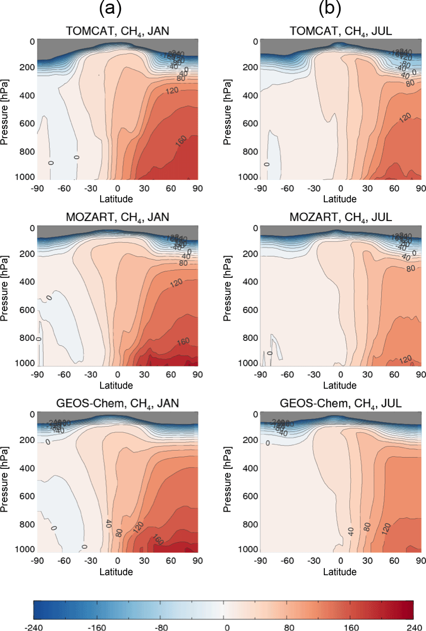
Figure 11 Zonal-mean distribution of CH₄ (ppb) for January (a) and July (b) 2011 in each of the GAUGE CTMs. For each model the concentration of CH₄ at the surface South Pole concentration is subtracted from the global distribution.

Although Bayes' theorem provides the basis for each of the inverse modelling techniques used in GAUGE, each approach employs a slightly different methodology to infer optimized surface fluxes. As we have already seen, there can be relatively large differences in atmospheric transport models. Indeed, the errors associated with atmospheric transport models are amongst the largest source of errors associated with estimating GHG fluxes (e.g. Locatelli et al., 2013; Miller et al., 2015).

In the interest of brevity, we only briefly introduce the inverse methods employed within GAUGE and refer the reader to dedicated papers on the techniques.

The global and nested GEOS-Chem model is linked with an ensemble Kalman filter (Feng et al., 2009, 2011, 2017). This approach does not require that we linearize the model but assumes approximate Gaussian statistics. The ensemble Kalman filter approach allows us to include easily estimates of model atmospheric transport error. Flux estimates are resolved in geographical regions informed by the ability of the data to independently estimate fluxes on those spatial scales. Over the UK, fluxes are estimated on pre-defined aggregated county levels and on a weekly scale. Weekly values are subsequently aggregated to longer timescales to minimize autocorrelation between successive flux estimates.

The inverse version of the TOMCAT model, INVICAT (Wilson et al., 2014), uses a variational inversion method based on 4D-Var. This approaches uses the adjoint version of the forward model to minimize the a posteriori fit between the model and data. This is an iterative method that can sometimes require a large number of iterations before convergence. Consequently, we resolve a posteriori emissions using TOMCAT at a spatial resolution of 2.8^∘.

Two inverse frameworks use the regional NAME dispersion information: (1) InTEM, a Bayesian inverse method building on Manning et al. (2011), and (2) a hierarchical Bayesian method in which the basis function, decomposition of the flux space, and the model and a priori uncertainties are explored using reversible-jump MCMC (Ganesan et al., 2014; Lunt et al., 2016). Both these models estimate emissions across a northwest European domain at horizontal resolutions from 25 to 100 km, depending on the frequency of sampling different regions. Boundary conditions are solved within each NAME inversion, following Ganesan et al. (2015) for InTEM and Lunt et al. (2016) for the MCMC approach. Monthly UK emission estimates of CH₄ and N₂O were estimated for the period 2013–2016 and compared to the reported inventory. For the MOZART model we used a hierarchical Bayesian method based on Ganesan et al. (2014).

Our GAUGE inverse model studies generally include a series of factorial experiments that allowed us to explore the relative importance of individual and collective data to estimate UK CO₂ and CH₄ flux estimates. Based on these experiments, we define a control experiment. We test the robustness of our results by comparing results from using half or double the assumed measurement uncertainties. UK a posteriori flux estimates for CO₂ and CH₄ are currently being prepared for publication: Lunt et al. (2018) and Palmer et al. (2018). Broadly speaking, we have estimated net CO₂ fluxes using regional and global scales but have been unable to attribute those fluxes to specific sectors; for CH₄, using the continental-scale data and the regional network data, we have begun to improve our understanding of sector emissions, and for N₂O, which has the small atmospheric gradients due to its long atmospheric lifetime, we have not begun to analyse the data collected within GAUGE.

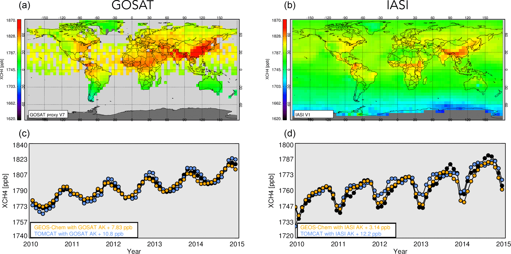
Figure 12 Seasonal mean dry-air column-averaged mole fractions of CH₄ (XCH₄) from (a) GOSAT and (b) IASI for June–August 2014, described on a regular $\mathrm{5}{}^{\circ }\times \mathrm{5}{}^{\circ }$ grid. The bottom rows show a global mean time series of XCH₄ for 2010–2015. The GEOS-Chem and TOMCAT models have been sampled at the time and location of individual measurements and convolved with scene-dependent averaging kernels prior to calculating the mean value.

4 Concluding Remarks

The main objective of the Greenhouse gAs Uk and Global Emissions (GAUGE) project was to estimate the magnitude, distribution, and uncertainty of UK emissions of three atmospheric greenhouse gases (GHGs): carbon dioxide (CO₂), methane (CH₄), and nitrous oxide (N₂O). To achieve that objective, we established an interlinked measurement and data analysis programme of activities from 2013 to 2015. These activities substantially expanded on existing measurements and data analysis. Some measurements that were established as part of GAUGE have continued beyond 2015. The primary motivation for GAUGE was to develop a measurement-led system to verify UK GHG emissions in accordance with the UK Climate Change Act 2008. GAUGE also lays the foundations for estimating nationally determined contributions as part of the Paris Agreement.

Emissions of CO₂, CH₄, and N₂O represented 97 % of UK GHG emissions during 2015 (the latest budget estimates available from the UK government). These emissions originate from a variety of sectors, including energy supply, transport, business, residential, agriculture, waste management, and other. These emissions are very different in nature, ranging from point sources to large-scale, diffuse sources. We considered this heterogeneity of course when we designed the GAUGE measurement programme.

The backbone of GAUGE is a network of measurements that are collected at height from telecommunication masts, tall towers, distributed across the UK. These measurements are typically collected at multiple inlet heights (100–300 m) above the local terrain (and sources) so they have a reasonable fetch suitable for quantifying sub-national-scale GHG fluxes. GAUGE added two tall-tower sites to the UK Deriving Emissions linked to Climate Change (DECC) tall-tower network. The DECC network was established in 2012 to estimate GHG emissions from the UK's devolved administrations. The GAUGE sites included a site on the North Yorkshire Moors, with sensitivity to the greater Manchester–Leeds–Liverpool–Sheffield region, and in East Sussex, which has sensitivity to emissions from London.

We collected data on a commercial ferry that travelled regularly between Rosyth, Scotland, and Zeebrugge, Belgium. This mobile measurement platform provided information on UK and mainland European outflow of GHGs, which complemented the tall-tower data. Using a regional tower network over East Anglia, comprising mostly measurements collected on church steeples, we found additional spatial and temporal flux distributions over the region could be achieved. We chose East Anglia because it is where there is a high density of agriculture and where the local terrain is relatively flat, so that church steeples often represent the highest local landmarks. As part of GAUGE we deployed the UK Atmospheric Research Aircraft for a limited number of flights around and across the UK. These data have been used to study the transport of atmospheric GHGs on local to regional spatial scales.

To explore how the UK GHG measurement network could develop in the future, we incorporated new technologies and new measurement platforms into the GAUGE programme. We deployed small sensors that were launched on a small number of sonde launches, which offer a potentially new way to obtain vertical distributions of GHGs. We also used unmanned aerial vehicles as part of a larger measurement campaign to characterize GHG emissions from a landfill, helping to pave the way for using this technology more generally within larger-scale GHG emission experiments. We also explored how we can use satellites effectively to estimate UK GHG fluxes. The spatial and temporal coverage of clear-sky measurements over the UK from current SWIR instruments, which are sensitive to changes in CO₂ and CH₄, is too sparse to provide competitive constraints on CO₂ fluxes. We anticipate this situation will slowly change with new instruments (e.g. TROPOMI) and proposed mission concepts (e.g. Copernicus CO₂ service) that will result in higher spatial resolution and consequently more cloud-free scenes.

We used a range of global and regional atmospheric transport models linked with inverse methods to interpret the atmospheric GHG observations. We showed that these models have skill in reproducing observed atmospheric CO₂ and CH₄ variations on hemispheric scales but disagree with N₂O observations due to much smaller gradients that reflect its longer atmospheric lifetime. This multi-model approach was adopted to help study the model spread in a posteriori GHG fluxes and to study the relative importance of individual data to estimate UK GHG fluxes. For this work, we refer the reader to the dedicated papers.

We approached source attribution in two ways. First, we used the regional-scale network to improve the distribution of CH₄ fluxes due to agriculture, taking advantage of reasonable spatial disaggregation of this source over East Anglia. We also established an isotope measurement programme, including concurrent measurements collected at Mace Head, Ireland, and Tacolneston, East Anglia. Data from these two sites provided a crude meridional gradient over the UK. Our sampling approach was designed, using the prevailing wind direction over the UK, to determine the gradient due to fossil fuel CO₂. Despite our best efforts, neither approach to source attribution was definitive. For example, our analysis of radiocarbon was compromised by the influence of the nuclear power sector. We anticipate the development of a more optimal sampling approach is possible by working more closely with this sector to avoid instances when sampled air masses are dominated by upwind nuclear sources.

GAUGE represents a first concerted attempt by the UK science community to quantify nationwide GHG fluxes. We have laid the foundations of measurement infrastructure that moves forward with a better understanding of the advantages and disadvantages of individual GHG data. The post-GAUGE tall-tower network has continued. For instance, the UK DECC network has adopted the North Yorkshire site, which provides valuable flux information about northern England and to a lesser extent southern Scotland, and the National Physical Laboratory now runs the tall tower at Heathfield. We also anticipate a growing role for satellite observations, which are free at the point of delivery, as new instruments provide better spatial coverage and probabilistically a higher number of cloud-free scenes. Data analysis will continue as improved models and inverse methods progressively better describe the physical and chemical processes that determined atmospheric GHGs. The UK is a geographically small country and plays a proportional role in the Paris Agreement, but we expect the design of GAUGE can be scaled upwards to larger geographical regions, taking advantage of specific technologies relevant to the sectors that dominate continental GHG budgets.

Appendix A: Tall-tower site descriptions

Table 1 describes the basic characteristics of each site. The MHD atmospheric research station is situated on the west coast of Ireland. MHD receives well-mixed air masses from prevailing southwesterly winds across the North Atlantic (on average 37 % of the time; Grant et al., 2010), providing a good mid-latitude Northern Hemisphere background signal. The resulting time series provides an essential baseline for the combined UK GHG measurement network. The area immediately surrounding MHD is generally wet and boggy with areas of exposed rock and is sparsely populated with very low associated anthropogenic emissions (Dimmer et al., 2001). The closest city to MHD is Galway, which lies 55 km east of MHD and has a population of 75 000.

RGL is a rural UK site located 30 km from the border of England and Wales. It is 16 km southeast of Hereford (population 55 800), and 30 km southwest of Worcester (population 98 800) in Herefordshire, UK (Office for National Statistics, 2012). The land surrounding the tower is primarily used for arable, livestock, and mixed farming purposes (Department of the Environment and Rural Affairs, 2010a). There are 25 wastewater treatment plants within a 40 km radius of the site, the majority of which are in the northeast to southeasterly wind sector (Department of the Environment and Rural Affairs, 2010b). A landfill site lies 30 km to the east of the site.

TAC is a rural UK site located near the east coast of England. It is 16 km southwest of Norwich (population 200 000) and 28 km east of Thetford (population 20 000) in Norfolk, UK (Office for National Statistics, 2012). Land surrounding the tower is primarily used for agriculture, which is dominated by arable farming (Department of the Environment and Rural Affairs, 2010a). There are three landfill sites between 30 and 50 km from the site, the closest being 30 km to the east (NCC, 2013). There is also a poultry litter power station in Eye, 20 km south of the site.

TTA is a rural UK site located near the east coast of Scotland. It is 10 km north of Dundee (population 148 000; General Register Office for Scotland, 2013). Land surrounding the tower is predominantly under agricultural use, primarily livestock farming due to its hilly terrain.

HFD is located in rural East Sussex, 20 km from the coast, and surrounded by woodland, parkland, and agricultural green space. The closest large conurbation, Royal Tunbridge Wells (district population 264 000; Office for National Statistics, 2012), is located 17 km NNE from the tower, while greater London is 40 km NNE.

BSD is a remote moorland plateau site within the North Yorkshire Moors National Park. It is 25 km NNW of Middlesborough (the closest large urban area, population 139 000; Office for National Statistics, 2012) and 30 km from the coast.