the Creative Commons Attribution 4.0 License.
the Creative Commons Attribution 4.0 License.
 | 31 Jul 2018
Impact of gravity waves on the motion and distribution of atmospheric ice particles
Aurélien Podglajen
Riwal Plougonven
Albert Hertzog
Eric Jensen
Gravity waves are an ubiquitous feature of the atmosphere and influence clouds in multiple ways. Regarding cirrus clouds, many studies have emphasized the impact of wave-induced temperature fluctuations on the nucleation of ice crystals. This paper investigates the impact of the waves on the motion and distribution of ice particles, using the idealized 2-D framework of a monochromatic gravity wave. Contrary to previous studies, special attention is given to the impact of the wind field induced by the wave.
Assuming no feedback of the ice on the water vapor content, theoretical and numerical analyses both show the existence of a wave-driven localization of ice crystals, where some ice particles remain confined in a specific phase of the wave. The precise location where the confinement occurs depends on the background relative humidity, but it is always characterized by a relative humidity near saturation and a positive vertical wind anomaly. Hence, the wave has an impact on the mean motion of the crystals and may reduce dehydration in cirrus by slowing down the sedimentation of the ice particles. The results also provide a new insight into the relation between relative humidity and ice crystals' presence.
The wave-driven localization is consistent with temperature–cirrus relationships recently observed in the tropical tropopause layer (TTL) over the Pacific during the Airborne Tropical Tropopause EXperiment (ATTREX). It is argued that this effect may explain such observations. Finally, the impact of the described interaction on TTL cirrus dehydration efficiency is quantified using ATTREX observations of clouds and temperature lapse rate.
- Article
(8190 KB) - Full-text XML
- BibTeX
- EndNote


Atmospheric gravity waves have long been reckoned to interact with cirrus clouds. They generate temperature fluctuations, with negative anomalies favoring ice particle formation (Potter and Holton, 1995). High-frequency gravity waves influence the cooling rates undergone by air parcels, which has an overwhelming impact on the properties of newly nucleated clouds (Dinh et al., 2016; Jensen et al., 2010, 2016; Spichtinger and Krämer, 2013). So far, most studies investigating the impact of waves on ice clouds have been focusing on temperature anomalies. However, gravity waves also have a wind signature, and might move around sedimenting ice particles in a different way than they do air parcels. This in turn could modulate the lifetime of the crystals, but also the efficiency of dehydration by cirrus. Indeed, dehydration is achieved when ice crystals grow and travel a significant distance on the vertical before they start to sublimate (Dinh et al., 2014; Podglajen et al., 2016b). Depending on whether the vertical winds induced by the waves are opposing or accelerating the sedimenting motion of the particles, they might diminish or enhance the efficiency of water redistribution by sedimentation.
The goal of this paper is hence to examine the influence of internal gravity waves on ice crystal transport. Motivated by recent observations of wave–temperature relations in the tropical tropopause layer (TTL) by Kim et al. (2016), we focus on the temperature range of TTL cirrus clouds (around 190 K). However, the theory presented is general and might apply to a number of aerosol particles present in different regions of the atmosphere affected by gravity waves, including particles in polar stratospheric clouds, noctilucent clouds in the mesosphere, or even stratospheric aerosols. Incidentally, the study will also bring a deeper insight into the relation between relative humidity and ice crystals' presence.
The article is organized as follows. In Sect. 2, a simplified setting is used to investigate the wave impact on ice crystal transport analytically. Then, in Sect. 3, the relevance of the analytical results is tested using numerical simulations and the impact of the described effect is investigated in observations of TTL cirrus during the Airborne Tropical TRopopause EXperiment (ATTREX). Implications are discussed in Sect. 4. Finally, Sect. 5 provides the conclusions.
To leading order (i.e., neglecting nonlinearities), propagating waves are not expected to affect transport, as they reversibly slosh fluid parcels to and fro. Yet, the second-order Stokes drift (Andrews et al., 1987) can lead to irreversible transport. For internal gravity waves or for equatorial Kelvin waves in the Boussinesq approximation (neglecting the decrease in density with altitude), however, that Stokes drift term cancels out. There is no mean transport of a purely Lagrangian tracer by a monochromatic internal gravity wave. However, ice crystals (or aerosols) are not purely Lagrangian tracers. In the vertical, they fall relative to the surrounding air. Since the wave phase generally propagates downward (if the energy is to propagate up above wave sources), the falling particles fall in the direction of wave propagation. If the particles are falling at the same speed as the wave propagates downward, they will remain in the same wave phase and hence see a constant wind anomaly: thus, there is potentially a systematic effect of the wave presence on the mean motion of the particles.
In the following, we use a simple 2-D framework with the wind and temperature structure of a monochromatic wave within an unsheared background to examine the potential effects of the wave on ice crystals' transport. In order to simplify the notations without loss of generality, we furthermore assume that there is no background wind. In this idealized setup, there is an exact analytical solution for the wave disturbance, which renders analytical progress possible. Furthermore, despite this idealization, the assumptions are not completely unrealistic: although shear can be large in the atmosphere, a significant part of it can be attributed to the waves themselves rather than to the background flow (Podglajen et al., 2017); quasi-monochromatic waves have long been observed in the atmosphere, such as Kelvin waves in the TTL (Boehm and Verlinde, 2000; Wallace and Kousky, 1968), gravity waves in the mesosphere (Rapp et al., 2002), or mountain waves in the upper troposphere and stratosphere. We would also like to emphasize that the qualitative results obtained through the investigation of this idealized case are based on robust properties of the wave–ice crystal system and probably apply to more complex flows.
2.1 Constant size particle
First, consider the case of a constant size particle, which is assumed to sediment vertically with a downward speed vsed > 0. The evolution of the particle's position X(t), Z(t) is then given by the following:
where U and W are the amplitude of the wave in horizontal and vertical wind respectively, ω is the angular frequency, k is the horizontal wavenumber, m is the vertical wavenumber, and ϕ is the wave phase. Note that we consider a gravity wave in the midfrequency range (f ≪ ω ≪ N with f the local Coriolis frequency and N the Brunt–Väisälä frequency), so that the polarization relations (Fritts and Alexander, 2003) impose that the wave horizontal wind perturbation is aligned with the horizontal wavenumber. The 2-D plane x–z is chosen along the direction of propagation of the wave (and is not necessarily zonal). Near the equator (f → 0), these formulas also describe equatorial Kelvin waves and x–z is then a vertical–zonal plane. For both types of waves, the polarization relations also give the following:
Then, there is an analytical formula for the vertical trajectory Z(t) of the particle with initial position X0, Z0:
with ϕ0 = kX0 + mZ0 + ϕ. This analytical solution highlights the difference with a no-wave case, which would simply give Znowave(t) = −vsedt + Z0, but also with a Lagrangian air parcel, whose vertical position is given by the following:
As gravity waves in the upper troposphere mostly propagate from lower levels, their vertical group velocity is positive, which implies that their vertical phase speed = is negative (Fritts and Alexander, 2003). In the following, we take the convention ω > 0 so that a negative vertical phase speed is associated with m < 0. Depending on the ratio between and vsed, different cases may arise. If ≫ vsed, the particles follow the air parcels and oscillate vertically. The particles are close to perfectly Lagrangian, and there is no net effect of the wave. If ≪ vsed, the particles travel in a stationary wave field, i.e., through positive and negative wave phases, whose contributions cancel out in a long enough temporal average. The interesting interaction appears when and vsed are of the same order: then, as ω + mvsed < ω and ω + mvsed > mvsed, the variations seen by the particles have longer periods than those seen by air parcels or by particles that would fall through a stationary wave field with the same vertical structure. This is due to the fact that the particles travel in the same direction as the wave phase. In particular, when ≃ −vsed (for t ≪ ), one has the following:
and thus the wave can bring a significant contribution to the displacement of the crystal, a contribution which does not cancel out after one wave period. Such a configuration could also significantly modify the lifetime of the ice crystals, which could stay longer or shorter times in saturated or supersaturated regions than if only sedimentation were moving them. Since we only consider nonbreaking waves, it should be noted, however, that the vertical wind contribution cannot overcome sedimentation in the long-term because stability requirements impose that W < ≃ |vsed| (see Appendix A). Furthermore, Eq. (6) implies a significant contribution of the wave to the motion of an individual ice crystal, but not necessarily an average effect on the ice crystal population. Indeed, if there is no preferential location of the crystals in the wave phases ϕ0 then some crystals are accelerated but others are slowed down.
For illustration, we show the effect of a monochromatic wave on the vertical motion of falling particles in a special configuration in Fig. 1. We assume that the particles fall at a constant speed of 2 cm s−1 (equivalent to a ≃ 20 µm diameter spherical ice particle at T = 190 K and P ≃ 120 hPa). The wave is chosen with a period T = ≃ 1 day, a shallow vertical wavelength λz = = 4 km. The chosen squared Brunt–Väisälä frequency is = 2 × 10⁻⁴ rad2 s−2, i.e., intermediate between the stratosphere (where = 4 × 10⁻⁴ rad2 s−2 typically but can be as large as 1 × 10⁻³ rad2 s2) and the troposphere (where typically = 1 × 10⁻⁴ rad2 s−2 but can be smaller near the bottom of the TTL), as expected for the transition region of the TTL. The horizontal wavelength is prescribed from the dispersion relation: λx = = ≃ 800 km. The Eulerian temperature perturbation has an amplitude AT = 1 K, so that the vertical velocity amplitude is equal to
with g = 9.81 m s−2, = 185 K, and U = ≃ 3.7 m s−1. Overall, the chosen wave characteristics are similar to those of equatorial waves commonly observed in radiosondes (Kim and Alexander, 2015). Although the only requirement for a significant effect on the particle's speed is that the fall speed of the particle is close to the vertical phase speed of the wave, the integrated effect on the particle's displacement will be larger for low-frequency waves, such as the one chosen in this example.
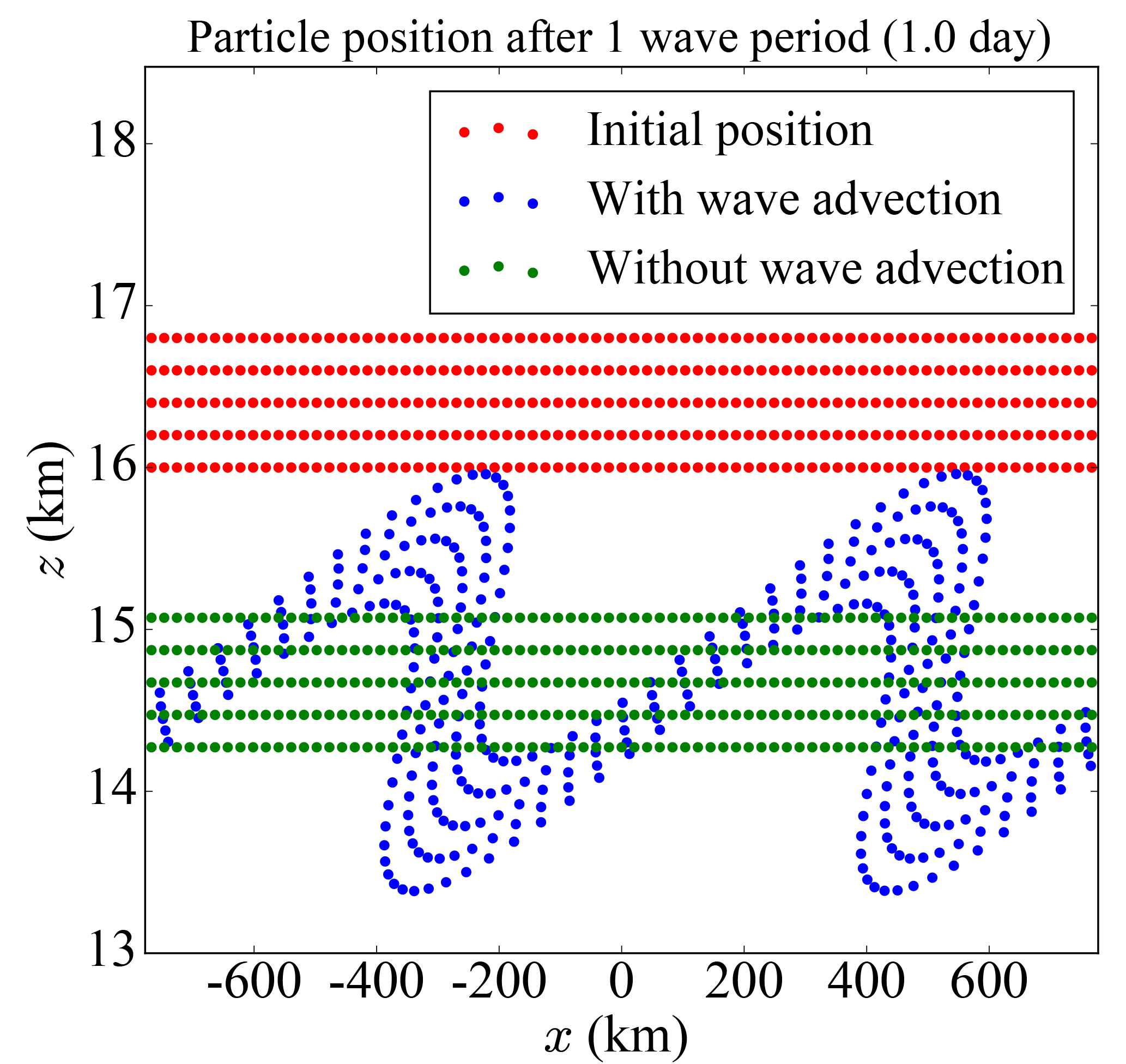
Figure 1Evolution of the positions of sedimenting particles (initial positions in red) being advected by the wind field induced by a monochromatic wave (blue dots) or not (green dots) during one wave period. See text for a full description of the wave characteristics. Also note that the vertical scale has been enhanced by a factor of about 200 compared to the horizontal scale.
Figure 1 shows the initial positions of the particles (red dots) and their positions after one wave period (blue dots), so that all meteorological fields have the same value as at the beginning and the air parcels have returned to their initial positions. However, the particles have descended in altitude due to sedimentation. Without the wave, the particles would just fall to the green positions. Due to the presence of the wave, advection by the vertical and horizontal winds significantly disperses the particles vertically relative to the no-wave case. Although we did not select the wave characteristics other than the intrinsic frequency to obtain it, a significant impact can be expected. We also checked that the monochromatic wave was stable (see Appendix A).
Consistent with Eq. (6), Fig. 1 shows that if the particles are of constant size with vsed ≃ , there is a significant impact on the motion of individual particles. However, if the particles are initialized in all phases of the wave, there is no effect on the mean downward transport of the particles' population. The main impact is to disperse the particles vertically with some particles falling more slowly but others falling more rapidly when the wave is present. Which of the two (increased or suppressed fall of the particles) will prevail in a realistic setting (i.e., including growth and sublimation)?
2.2 Growing and sublimating ice crystals and wave-driven localization
2.2.1 Governing equations
Now that we have explored the impact of wave advection on particle transport, we turn to the case of ice crystals which can grow and sublimate, exchanging water molecules with their environment. We will not, however, consider the effect of the ice crystals on the relative humidity, equivalent to assuming that few of them are present. Consistently, we will neglect ice crystal aggregation; diffusional growth and sedimentation are thus the only microphysical processes active in our setup.
For crystals with a spherical shape, the rate of growth of the radius r is given by Pruppacher and Klett (1978):
with RHi = the relative humidity with respect to ice (q being the volume water vapor mixing ratio and qsat the volume saturation mixing ratio with respect to ice) and G′(r, T; αd) the growth factor, a function of temperature T, the crystal radius r and the deposition coefficient αd, given by the following:
where ρice = 918 kg m−3 is the density of ice, is the modified diffusivity of water vapor in air, is the modified thermal conductivity of air, esat is the saturation water vapor pressure, Rv = 462 J K−1 kg−1 is the gas constant for water vapor and Ls = 2.844 × 10⁶ J kg−1 is the latent heat of sublimation of ice. The modified diffusivity can be expressed as the product of the diffusivity Dv(T) and the ventilation coefficients fd,v(r, T) (for large ice crystals) and nonequilibrium corrections fd,k(r, T; αd) (for small ice crystals). Similarly, the modified thermal conductivity is the product the conductivity ka(T) and the coefficients fk,v(r, T) and fk,k(r, T):
Expressions for the f coefficients can be found in Pruppacher and Klett (1978). For intermediate crystal sizes (r ≃ 5 to 50 µm) and large deposition coefficients (αd ≥ 0.5), ≃ Dv(T) and ≃ ka(T), in which case G′ also is a function of T only. The exact value of the deposition coefficient αd, which represents the fraction of water molecules colliding with the ice surface that effectively get incorporated into the ice crystal lattice, is not known. It could well vary with supersaturation or temperature and take any value from 0.001 to 1, and experimental studies have not been very helpful in constraining it so far (Magee et al., 2006; Skrotzki et al., 2013). However, atmospheric cloud observations are hard to reconcile with αd values smaller than about 0.5 (Kay and Wood, 2008; Kärcher and Lohmann, 2002), and the recent discussion by Skrotzki et al. (2013) also recommends 0.2 ≤ αd ≤ 1. We assume αd=0.5, consistent with that literature. We note that the results presented below are not sensitive to the precise value of αd as long as it is sufficiently large (larger than ∼ 0.5), since G′ is then essentially a function of temperature only. However, for smaller values of αd, G′ depends both on r (below some size up to tens of microns) and αd, and the results may be significantly altered both quantitatively and qualitatively.
In the following, we introduce G = 2 G′, the rate of growth of the squared radius. The governing equations for the evolution of the ice crystal size and position in the monochromatic wave field are then as follows:
where again X(t) and Z(t) are the particle's horizontal and vertical positions. Of course, the trajectories of the crystals are irreversibly stopped when they fully sublimate (r = 0).
To solve these equations, we need to know the temperature and relative humidity at the position X(t), Z(t) of the ice crystals. For the temperature, we could have used the polarization relations (Fritts and Alexander, 2003), but it is actually more relevant to derive T and RHi directly by considering the field of vertical displacement induced by wave. Since we assume a monochromatic wave, the temperature T(x, z, t) at any fixed (Eulerian) position (x, z) in space is that of the air parcel that has been adiabatically displaced to (x, z) by the wave. Noting Zwave(x, z, t), the vertical component of this displacement, we have
where is the undisturbed (background) temperature at the air parcel equilibrium altitude . Hence,
In the formulas above, the vertical displacement is given by the following:
Regarding the pressure P, which is required in the relative humidity to evaluate the volume saturation mixing ratio qsat = , we assume hydrostatic equilibrium in the reference state and neglect the pressure perturbations induced by the wave: P(x, z, t) = . (Note that this is consistent with Eq. 15, which neglects the contribution of Eulerian pressure anomalies to temperature changes.)
Regarding the water vapor mixing ratio, as mentioned above, it is estimated assuming that the crystals do not significantly deplete the water vapor content, which is then conserved. This last assumption will allow the wave–sedimentation interactions to be revealed more clearly. It is valid when the ice crystal number concentrations are small, which is common in thin TTL cirrus (Jensen et al., 2013; Krämer et al., 2009), sometimes also referred to as ultrathin tropical tropopause clouds (Peter et al., 2003). Indeed, Krämer et al. (2009) have argued that the relaxation time for supersaturation in those thin TTL clouds could be larger than a few hours. Furthermore, we assume that in the reference state the water vapor mixing ratio depends only on the vertical position, so that the water vapor mixing ratio at any position and time is given by the following:
For the reference-state profile, we choose to keep a constant relative humidity with altitude, RH, i.e.,
This setup retains the main characteristic of water vapor variability in the TTL, i.e., its decrease with altitude due to the decrease in saturation vapor pressure.
Finally, for the sedimentation speed vsed for spherical ice crystals, we will use the formulas provided in Pruppacher and Klett (1978), which are based on dimensional analysis and experiments, to evaluate the Reynolds number and then deduce the fall velocity of the particles. For particles' radii between about 5 and 100 µm, those formulas give results close to the one obtained assuming Stokes' flow (within 8 %), i.e.,
where μ(T) is the dynamic viscosity of air. However, for smaller particles, the formulas take into account the Cunningham correction, which corrects for the noncontinuum nature of the fluid for small particles. At the other end of the size spectrum, for particles larger than about 100 µm, the Stokes flow hypothesis is no longer valid and Eq. (20) overestimates the sedimentation speed, which is partly corrected in the formulas provided in Pruppacher and Klett (1978). We note also that those can be extended to nonspherical particles (Heymsfield and Westbrook, 2010; Mitchell, 1996), but this will not be used in the simulations since we here consider spherical crystals in the growth calculations. Observations also suggest that most of the smallest ice crystals in TTL cirrus clouds are quasi-spherical (McFarquhar et al., 2000); Lawson et al. (2008) found that most of the crystals with maximum dimension (2 r) below 65 μm were quasi-spherical. However, the crystals above 65 µm observed by Lawson et al. (2008) mostly had aspherical shapes (including hexagonal and disk-like). The dependency of the fall speed and therefore the mass flux on the particle shape is an important factor to take into account, and this will be discussed in Sect. 4.2.
2.2.2 System analysis
The previous set of equations will be the base for the simulations presented in Sect. 3.1. However, in order to analyze the dynamics of the system theoretically, we here consider three additional simplifications. First, we linearize the relative humidity term to only retain the essential oscillatory behavior (a strong, yet enlightening assumption given the non linearity of the saturation vapor pressure):
Second, we keep only the dependence on in G. This might induce some quantitative change, but the qualitative impact will be marginal.
Third, we use for vsed the simplified Stokes flow hypothesis from Eq. (20). This expression disregards corrections for small particles and large particles, but simplifies the algebra, since r2 intervenes in that expression and in the growth expression.
Under those additional approximations, the system of Eq. (14) can be rearranged into two ordinary differential equations for the wave phase Ψ = kX + mZ − ωt + ϕ along the ice crystal trajectory and for the squared radius of the particle r2, namely,
or, in a more abstract form,
This set of equations reveals the simple properties of the system studied. It can be seen that the system has fixed points, characterized by =0 and = 0, provided the following constraints are satisfied:
and
Then, there are 1 or 2 (depending if it is an equality or a strict inequality in the previous equation) fixed points, which are given by the following:
The first equation states that the sedimentation speed at the fixed point is equal to the wave vertical phase speed (vsed(rf) = ). The second equation states that RH = 100 %, i.e., the fixed points are located where the environment is exactly at saturation so that the ice crystals' radii are constant (this is also true in the full system, as can be seen in the last equation of Eq. 14). Note that the second equation in Eq. (26) corresponds to two possible fixed points in the wave phase space, since sin(Ψf) = sin(π − Ψf).
To gain further insights into the behavior of the trajectories in the vicinity of the fixed points, it is common to examine the linearized system. The Jacobian matrix at the fixed points is as follows:
and its eigenvalues λ verify
with the plus sign corresponding to Ψf in .
Given those eigenvalues, the two fixed points of the system deduced from the theoretical analysis are as follows:
-
A saddle point, for which λ2 > 0 and the two eigenvalues are reals of opposite signs. The value of the phase at the saddle point Ψs is characterized by Wcos(Ψs) < 0 (given that < 0), so that the vertical wind anomaly induced by the wave w′ is negative. The particles initially around that fixed point move away from it with hyperbolic trajectories in the Ψ–r space.
-
An elliptic point, for which λ2 < 0 and the eigenvalues are both purely imaginary and conjugate to each other. This fixed point is located in the cooling phase of the wave, i.e., its phase Ψe is characterized by a positive vertical wind anomaly: w′ = Wcos(Ψe) is positive. In the fully linear system one would expect periodic trajectories in the neighborhood of the elliptic point, with particles cycling periodically around it, at a frequency of
However, since the real part of both eigenvalues is zero for this point, the linear analysis is actually not sufficient to conclude regarding the behavior of the trajectories in the nonlinear system (Hirsch et al., 2013).
The linear analysis above only provides qualitative insights into the system behavior near the saddle point and cannot be applied rigorously near the elliptic point. However, the behavior of the system can still be studied further in a theoretical sense, since it turns out to be Hamiltonian (see Appendix B). The Hamiltonian function H can be expressed as
The trajectories in the r–Ψ space correspond to lines of constant H. This formulation makes it clear that there are periodic trajectories around the elliptic point iif . Indeed, in that case, the elliptic point is a local extremum of H (see Appendix B).
Figure 2 shows the phase portrait of the system (trajectories of the particles in the Ψ–r phase space, i.e., contours of constant H) for different background relative humidity RH. In this figure, only the part of the trajectories corresponding to r ≥ 0 are shown, since for r = 0 the crystals have fully sublimated and r < 0 has no physical meaning. The characteristics of the wave and of the background state that have been used in this figure are summarized in Table 1; unless stated otherwise, they will also be assumed in the remainder of the study. Although the wave temperature amplitude may seem large (1.7 K), they correspond to the large events that regularly occur in the TTL, as observed by Kim and Alexander (2013). In particular, one specific wave event observed near Guam during ATTREX was observed to induce larger zonal wind and temperature fluctuations, with a comparable period to the wave chosen here (Kim, 2015, also see the case study in Podglajen et al., 2017).
Table 1Wave and background state characteristics assumed for the sedimentation–growth simulations reported in this section. : average pressure (for the simplified system), : average temperature (for the simplified system), : background Brunt–Väisälä frequency, : wave period, λz: wave vertical wavelength, AT: wave (Eulerian) temperature amplitude, W: wave vertical wind amplitude, U: wave zonal wind amplitude, : wave vertical phase speed, : period of the oscillations of the crystals around the elliptic point (Eq. 29).


Figure 2Panels (a) and (c): representation in the Ψ–r phase space (phase portrait) of ice crystals' trajectories (blue lines) obtained with wave parameters given in Table 1 for two different background relative humidities: a moist case similar to the western Pacific (RH = 0.85, a) and a drier case similar to the eastern Pacific (RH = 0.63, c). These trajectories correspond to constant values of the Hamiltonian function (Eq. 30). Black arrows along the blue lines indicate the trajectory direction. The vertical heavy line corresponds to rf, the particle radius at the fixed points. The heavy horizontal black lines show the location of the wave phase of the elliptic (solid) and saddle (dashed) fixed points. The heavy red lines limit the area around the elliptic fixed point where the crystals have “perpetual” periodic trajectories. It should be noted that the y axis (Ψ) is similar to a vertical profile, with decreasing Ψ corresponding to increasing altitude (since m < 0); the corresponding temperature anomaly profile due to the wave is sketched on (b).
Figure 2 emphasizes the existence of closed (periodic) orbits near the elliptic fixed points, located where RHi = 100 % in the cooling phase of the wave and delimited by the red lines. The crystals in that region remain in a specific phase of the wave near the elliptic point. We call this behavior of the crystals remaining in a specific wave phase the wave-driven localization of ice crystals. Furthermore, the figure emphasizes that crystals initially placed in the negative temperature anomaly region will tend to grow and leave that region to move into the positive temperature region, spending some time on the way in the cooling phase of the wave. Even if they are outside the region of permanent trapping near the elliptic point, some trajectories remain near that region for a significant amount of time, so that the preferential location of crystals due to the wave-driven localization might manifest itself for a fraction of the crystal population larger than that corresponding to the area enclosed by the red curves.
2.2.3 Physical understanding
The existence of the two fixed points can be easily understood physically. The elliptic point is located at RHi = 100 % and > 0. Hence, if ice crystals fall below that fixed point, they fall into subsaturated air (RHi < 100 %) and sublimate, which reduces their mass and their fall velocity. They fall more slowly and are caught up again by the wave phase which is also descending. They may then be transported into supersaturated regions where they grow, increasing their weight and fall speed and moving them back into the equilibrium phase. The trajectory of an ice crystal in altitude–time space around the elliptic fixed point is sketched in Fig. 3, to illustrate the previous explanation. It can be noted that the ice crystal cycles around the elliptic point with a period of about 12 h, consistent with Eq. (29) (see also Table 1). At the saddle fixed point, the reverse feedback is acting with subsaturated air above and supersaturated air below, so that the crystals move further away from this equilibrium point.
In many aspects, the mechanism presented here is similar to the stabilization mechanism proposed by Luo et al. (2003) to explain the existence of ultrathin tropical tropopause clouds. Those authors considered ice crystals in a stationary vertical wind and relative humidity profile, and they neglected the horizontal wind shear so that only vertical motions were examined. Then, a system of equations similar to Eq. (22) can be derived to describe the evolution of the crystal radius and position, in which essentially the altitude replaces Ψ and the vertical wind replaces the vertical wave phase speed. In that framework, for the same reason explained above for the elliptic point, ice crystals are stabilized in regions where RHi = 100 %, and > 0 provided the vertical wind is constant or decreasing with altitude. Taking a vertical profile, the location where the wave-driven localization occurs in our analysis (i.e., the elliptic point) is thus the same as the one where the stabilization effect of Luo et al. (2003) is expected (RHi = 100 %, > 0). However, since waves essentially dominate the variability of the vertical wind in the TTL, the setting of the quasi-monochromatic wave considered above is likely more realistic than the stationary vertical wind profile without horizontal wind shear used by Luo et al. (2003).
Returning to the location of the elliptic point where the crystals are localized, it should furthermore be noted that, given the tendency of some of the crystals to stay near the thermodynamic equilibrium phase of the wave (i.e., RHi = 100 %), there is for those a net impact of the wave on their vertical displacement. Indeed, at the elliptic fixed point, the crystals will endure a constant wave-induced horizontal velocity Ucos(Ψf) and a constant vertical velocity Wcos(Ψf). Since the elliptic fixed point is the one for which Wcos(Ψf) > 0, the consequence is that sedimentation is slowed down by wave advection.

Figure 3Representation in altitude–time space of an ice crystal trajectory in the moist (RH = 0.85) simulations. The colors correspond to the temperature anomaly profiles induced by the wave at the X position of the crystal, which also correspond to relative humidity anomalies. It is important to note that as a consequence of the crystal horizontal motion the X position at which the profiles are taken changes with time. The black line corresponds to the ice crystal trajectory and the circular markers represent the ice crystal size. Blue circles indicate growing ice crystals (RHi > 1), whereas red circles indicate sublimating ice crystals. Idealized trajectories of growing (blue) and sublimating (red) crystals in constant RHi backgrounds are also shown for a pedagogic purpose in the lower left and upper right corners.
2.3 Sensitivity of the wave-driven localization
2.3.1 Moist versus dry environments
Figure 2 displays crystals' trajectories for two background relative humidities, a moist (RH = 85 %) and a dry (RH = 63 %) scenario. These two scenarios serve to provide an explanation for geographical differences in TTL cirrus clouds over the Pacific ocean recently reported by Kim et al. (2016). Using in situ observations, their study examined the relationship between TTL cirrus clouds and temperature anomalies during boreal winter time and found different relations between the tropical eastern and western Pacific. In the eastern Pacific, TTL cirrus clouds are tied to the cold phases of the waves (the minimum of temperature anomaly T′ in Fig. 2b). In the western Pacific upper TTL, cirrus clouds are more frequent in the negative vertical temperature gradient phase (ddz < 0; the cooling phase of the waves if they propagate upward). This difference between the eastern and the western Pacific is probably not due to differences in wave amplitudes or characteristics: indeed, observations suggest that the lower frequency waves responsible for the temperature fluctuations do not show a strong geographic variability within the equatorial region (Kim et al., 2016; Podglajen et al., 2016a).
Another reason could be the different mean relative humidities between the two regions, the convective western Pacific being moister on average than the dry eastern Pacific. Two different explanations relying on the different background humidities could then explain the observations. The first, proposed by Kim et al. (2016), is that in a moist environment smaller temperature perturbations are required to go over the supersaturation threshold for ice nucleation than in a dry environment. Hence, ice formation may happen in the cooling phase of the wave where temperature perturbations are smaller in the moist regions while only the coldest wave phases provide sufficient supersaturation for nucleation in the dry eastern Pacific. However, this explanation does not take into account the life cycle of the ice crystals. Figure 2 illustrates an alternative explanation based on the interaction of sedimentation and growth with the wave field: in the dry environment, the elliptic fixed point is located near the cold phase of the wave (T′ < 0) while in the moist environment it is in the cooling phase of the wave (ddz < 0). The wave-driven localization effect may therefore be responsible for the preferential location of ice crystals and clouds in specific phases of wave-induced disturbances, like those reported by Kim et al. (2016).
2.3.2 Sensitivity to wave parameters
Besides the strong sensitivity to the background relative humidity, it is also interesting to investigate qualitatively the sensitivity of the wave-driven localization to the wave parameters. One metric to quantify the relevance of wave-driven localization is the fraction of phase space ℱp in which ice crystals of radius r = rf are affected by that process, i.e., ℱp = ΔΨ∕(2π) where ΔΨ is the phase difference of the two points limiting the closed orbits region at r = rf.
From Appendix B and by looking at Fig. 2, it appears that the trajectory passing through the saddle point delimits the closed orbits, as long as it does not intersect the line r = 0. In the latter case, it is the trajectory passing through the point r = 0, Ψ = Ψe (Ψe being the location of the elliptic point) which is the limit of the region with periodic orbits. The mathematical constraints are detailed in Appendix B and the corresponding limits of the regions with closed orbits for the two relative humidities are shown by the red curves in Fig. 2.
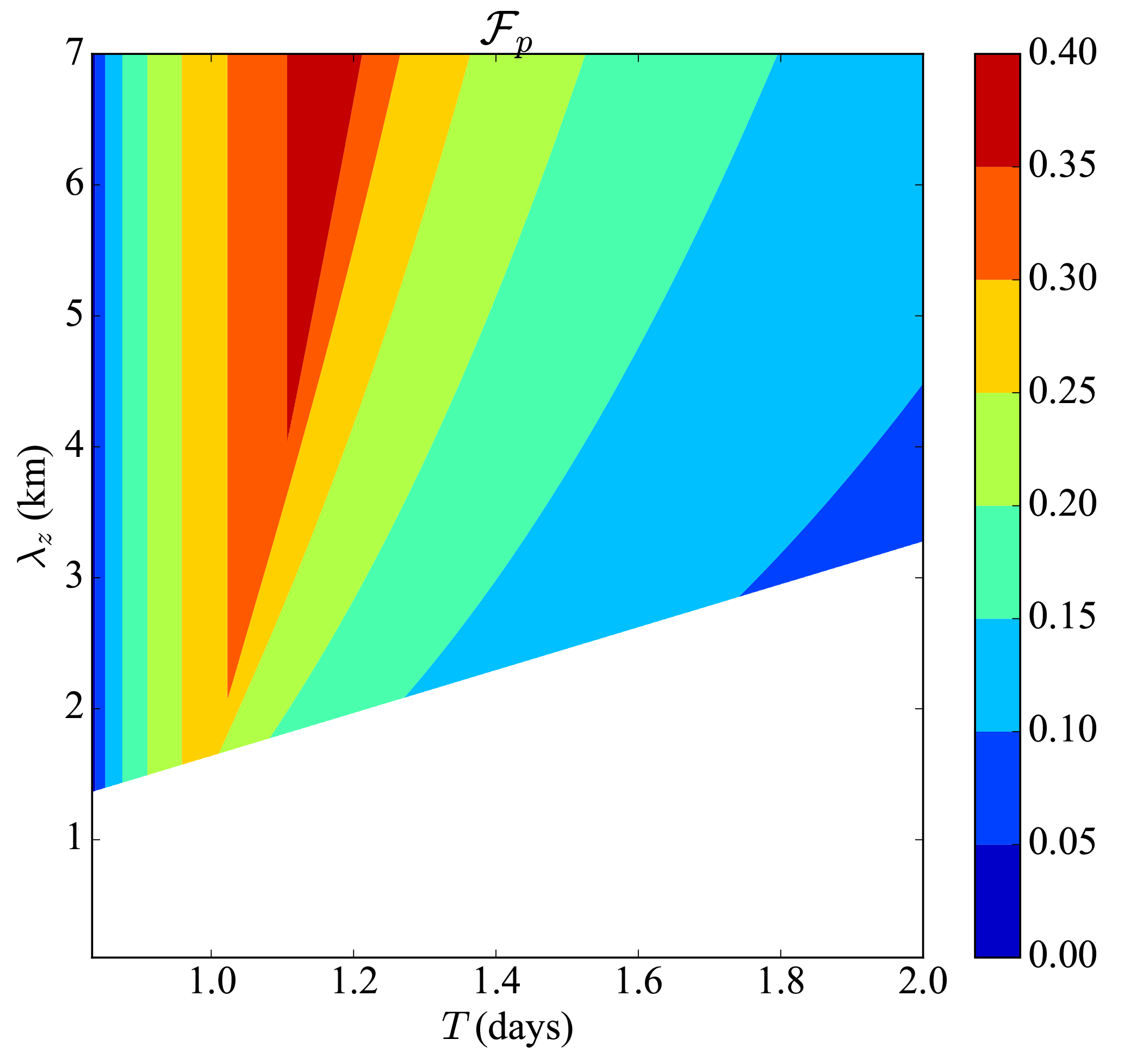
Figure 4Fraction ℱp of the wave phase space affected by the wave-driven localization, as a function of the period T = 2π∕ω and vertical wavelength λz = 2π∕m of the wave. RH = 0.85 and the parameters other than m and ω are given in Table 1. The regions of wave instability are not shown (white).
The dependency of ℱp to wave parameters is illustrated in Fig. 4 for RH = 0.85. This figure shows the existence of two regimes. In the first regime (wave periods below 1 day in that case), ℱp depends on the distance between the elliptic and saddle fixed points, and thus increases with the temperature amplitude of the wave (see Eq. 26). ℱp thus increases with the wave period T = 2π∕ω (it would also increase with W), with no dependency on the vertical wavelength λz = 2π∕m. This happens until the second regime is reached for larger periods. In this regime, ℱp is limited by crystals that fully sublimate. The wave parameters mainly act through modifying the radius at the fixed point (through vsed(rf) = = ), i.e., the position of the center of the orbits and their size. Hence, increasing λz increases ℱp mainly through an increase in rf, while increasing T decreases ℱp mainly through both a decrease in rf and an increase in the size of the orbits in r.
This exercise shows that low-frequency and large-vertical-wavelength waves are in general more susceptible to exhibit the wave-driven localization effect. However, it is quantitatively present (> 5 % of the wave phase space) for a large fraction of wave parameters, and is not restricted to the parameters chosen above.
In the previous section, a simplified framework was introduced to investigate the potential effects of the wave on ice crystal motions. The present section aims at confirming those effects with more realistic numerical simulations and to investigate them in observations.
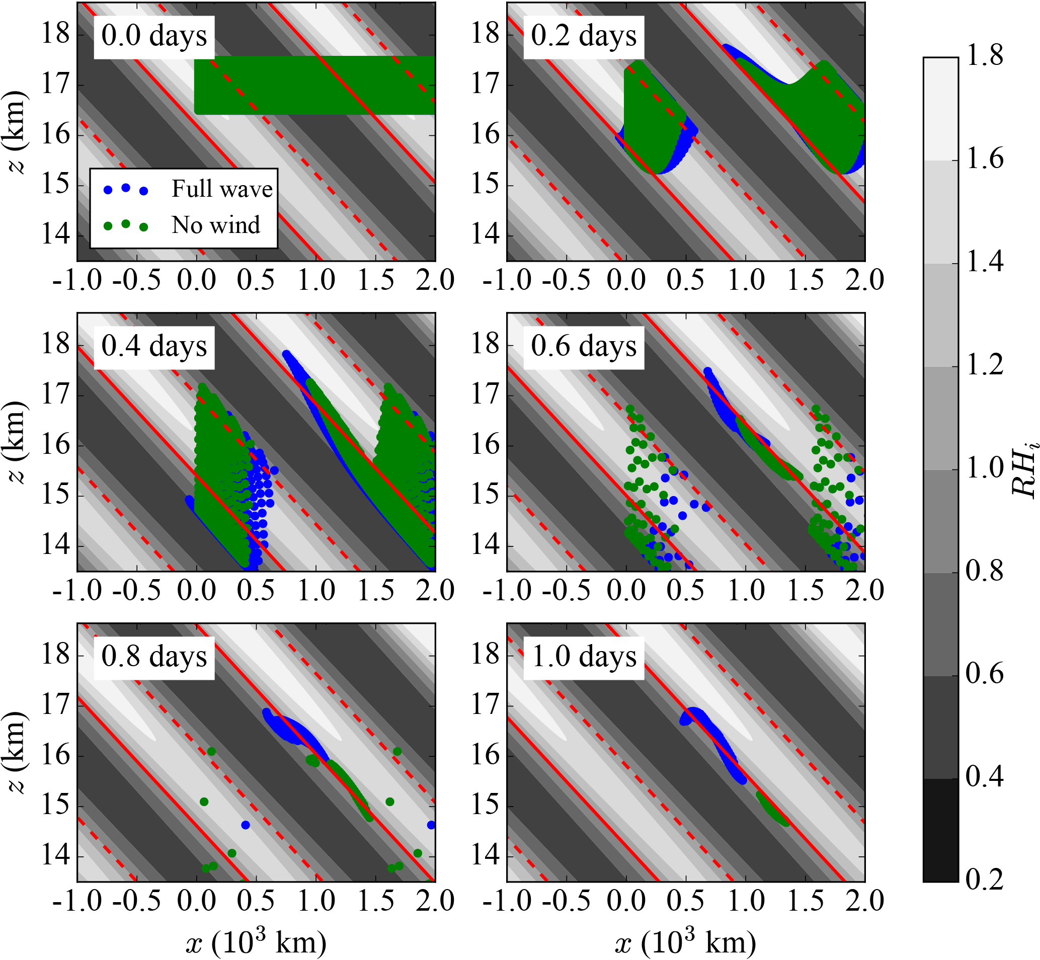
Figure 5Simulations of ice crystal growth and sedimentation in an idealized wave field at RH = 85 %. Different integration times are displayed, up to half a wave period, i.e., 1 day. The black and white background represents the RHi spatial variability and the colored dots correspond to the position of the ice crystals. The different colors correspond to simulations with different processes (un)accounted for: the blue dots represent the ice crystals' positions for the full simulation (wave advection and temperature fluctuations), whereas for the green dots both the horizontal and vertical winds induced by the wave have been neglected. The solid and dashed red lines respectively correspond to the locations of the elliptic and saddle points; for both of those RHi = 100 %. The initial ice crystal radius used for all crystals is 5 µm.
3.1 Full simulations
We now present numerical simulations of the full Eq. (14). The setup is the one presented in Sect. 2.2.1 (constant background relative humidity and idealized wave), but without the additional simplifications in Sect. 2.2.2. The full equations are solved, and the dependency of the microphysical parameters on the varying background temperature, pressure and crystal size are included. We still assume that there are few ice crystals, i.e., there is no water consumption. The goal is to extend the analysis of the simplified system, to check whether the expected patterns of cloud occurrence in preferred wave phases appear and to illustrate the impact of wave advection on transport. For that purpose, a population of ice crystals with radius 5 µm is initialized in all phases of the idealized wave. They then grow or sublimate depending on the environment's relative humidity. Sublimated ice crystals are irremediably lost, while the others continue their trajectories down to the bottom of the domain.
Figure 5 displays the results of a simulation at RH = 85 %, integrated during 1 day. The ice crystals are initialized with a radius of 5 µm around 17 km (16.5 to 17.5 km) in regularly gridded horizontal and vertical positions spanning all the phases of the wave. The different colors correspond to simulations accounting for wave advection or not, and will be discussed later.
Consistent with the analysis of the simplified system in Sect. 2 (see Fig. 2), three types of ice crystal behaviors are evident in Fig. 5 (blue dots):
-
Ice crystals initialized in (highly) subsaturated regions (RHi < 70 %, black in Fig. 5) quickly sublimate.
-
Ice crystals initialized in supersaturated regions below the saddle point grow and fall, and they cross the RHi = 100 % region (the elliptic fixed point) to sublimate below it, about half a vertical wavelength below their initial position.
-
Ice crystals initialized near the elliptic fixed point (RHi ∼ 100 %) tend to stay in the same wave phase and fall more slowly. This last group of ice crystals, which in this case amounts for about 5 % of the initialized crystals, tends to stay in the TTL for a significant amount of time after their initialization and may then be more frequently sampled during observations.
The qualitative behavior between the full ice crystal trajectories and the simplified system are thus similar. Now, is the remaining ice crystal population sensitive to the background relative humidity?
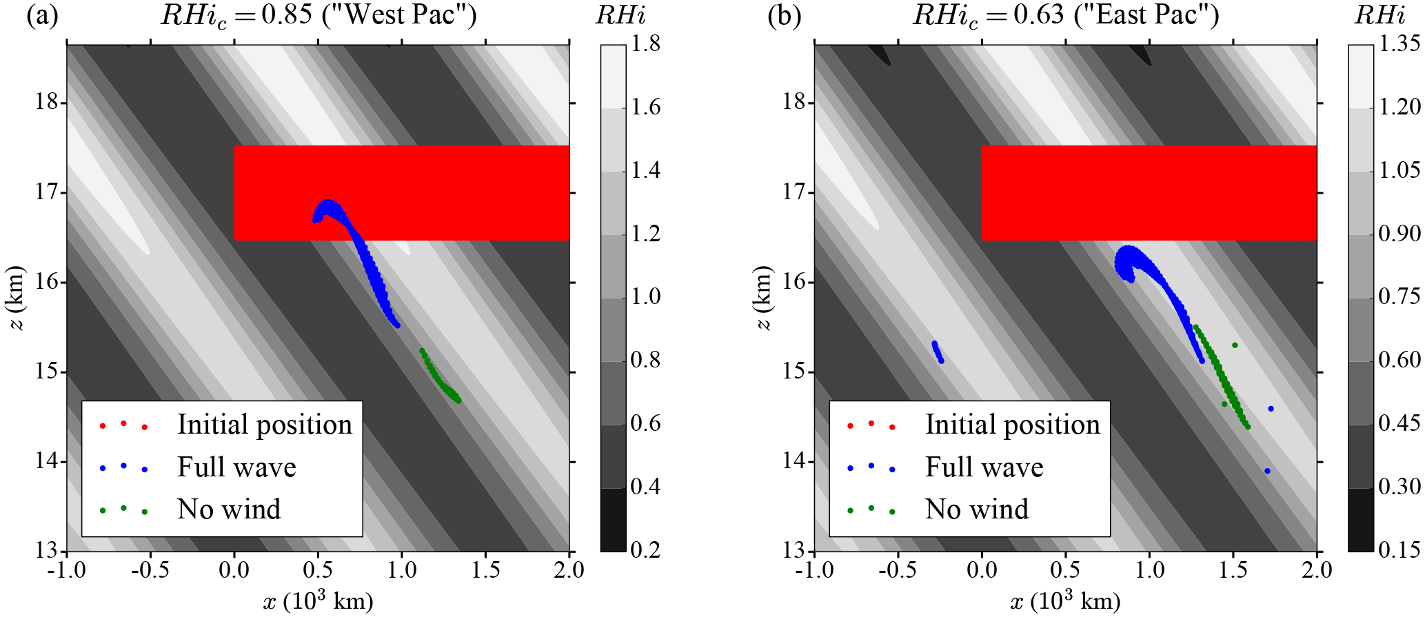
Figure 6Simulations of ice crystal growth and sedimentation in an idealized wave field at RH = 85 % (a) and RH = 63 % (b), after half a wave period, i.e., 1 day. Note that the scale for the relative humidity (background in black and white) differs between the two panels. Panel (a) is similar to the bottom right panel of Fig. 5. Dots represent the positions of the ice crystals, with the different colors corresponding to different trajectory simulations: the red dots are the initial positions of the particles and the blue dots represent the ice crystals' positions for the full simulation (wave advection and temperature fluctuations), whereas the green dots are ice crystals for which the wave-induced wind has been neglected in the simulation. The initial ice crystal radius used for all crystals is 5 µm. Note how the remaining crystals tend to be regrouped in the phase of the wave with RHi = 100 %.
In Fig. 6, the results of the previous simulation (RH = 85 %) are compared with the dry case (RH = 63 %) after 1 day of integration, i.e., half a wave period. The end position of the crystals are shown by the blue dots. The main characteristics described in Sect. 2.3.1 can again be noticed, with the remaining ice crystals (about 5 % of the initialized crystals in both cases) preferentially encountered where the relative humidity is near 100 % and in the < 0 ( > 0) phase of the wave. We also note that, in the dry case (Fig. 6b), there are remaining crystals after half a wave period even though those were not initialized in the region of perpetual oscillations expected from the theoretical analysis (their radius of 5 µm being too small, see Fig. 2c). They are, however, sufficiently close to this point to remain near the elliptic point a significant amount of time. Thus, due to the presence of the wave, those ice crystals can survive longer and remain in the TTL even though the large-scale state is subsaturated.
When the background relative humidity RH is increased even further (e.g., RH ≥ 100 %), the impact is similar with the remaining ice crystals near the elliptic point, which will be located at a different position in the phase such that RHi(Ψf) = 100 %. However, it should be noted that, for the ice crystals away from the elliptic point, the background relative humidity changes the relative proportion of ice crystals that sublimate versus those that quickly fall out of the TTL through the lower boundary of the domain.
In Sect. 2, we emphasized that ice crystals may encounter significant wave advection when they are more frequent in specific wave phases. The feedback between sedimentation and growth tends to localize the remaining ice crystals preferentially in the specific wave phase where the elliptic point is located. Hence, we can expect a mean impact on the downward velocity of the ice crystals.
To show that more precisely, we have also performed simulations without the wave advection. The crystals just fall, seeing the relative humidity perturbations created by the wave, but not the wave-induced wind perturbations. The end position of the ice crystals for the different simulations are represented in Figs. 5 and 6 by the green dots. For the low relative humidity case (RH = 63 %), the differences in the positions of the remaining ice crystals between the simulations with and without the wave-induced wind is limited, which is expected since the phase where the elliptic point is located in that case is characterized by very small vertical wind anomalies WcosΨe ≪ W. Yet, more crystals survive and do no sublimate in the full wind simulation than in the no-wind one (∼ 5 % vs. 1 %). In the high relative humidity setup, the differences between the full simulations and the no wind simulations already noticed for low RHi are enhanced: the downward sedimentation velocity of the crystals has been slowed down by almost a factor of 2, due to the crystals remaining in the phase WcosΨe ≃ W. This is in striking contrast with the simulation for which the wave wind was not accounted for.
The differences seen between these 2 simulations suggest that wave advection slows down the descent of the ice crystals. Indeed, when the full wave is appropriately accounted for, the crystals' downward motion at the elliptic point happens at a (negative) vertical speed:
whereas if the advection by the wave-induced wind is neglected, the crystals fall more rapidly and their downward vertical speed becomes larger (more negative), specifically
This is due to the fact that the vertical wind anomaly w′ = WcosΨe is positive at the elliptic point. Thus, the wave advection can significantly slow down the fall of ice crystals (in our example, by a factor of nearly 2). It is interesting to note that this effect does not only come from the wave-induced vertical wind but also from the horizontal wind disturbance, as detailed in Appendix C. The contribution of the wave to both wind components is thus central to entirely apprehend its impacts on ice crystals.
3.2 Quantifying the impact of wave advection on the vertical transport using observations
Overall, the experiments described above show that advection by the wave-induced wind has an impact on the sedimentation–growth of ice crystals and can significantly diminish the sedimentation mass flux, which suggests a mean impact of wave advection on the average dehydration efficiency of ice crystals. The downward water mass flux needed to close the water budget of the TTL may then be significantly affected by the waves. However, those simulations remain idealized: for instance, the described wave-driven localization is tied to the initialization of the crystals in all phases of the wave, in particular in the phase where RHi ≃ 100 %. Ice nucleation at low TTL temperatures is only active for RHi ≃ 120 % (heterogeneous nucleation) to 160 % (homogeneous nucleation) so that small-scale gravity waves superimposed to the large-scale wave would be required to bring all the air to the supersaturation threshold for nucleation. Given the number of additional assumptions and the complexity that would be required to represent them in a more complete setting, we leave those investigations in future work. Rather, to investigate the relevance of this potential effect to the atmosphere, we turn to aircraft observations in the TTL from ATTREX. In both 2013 and 2014 the Global Hawk carried a fast cloud droplet probe (FCDP) which was used to measure the size distribution and concentration of ice crystals from 1 to 50 µm diameter, and measured at about 1 Hz (180 m horizontal resolution). Temperature and pressure were provided at 1 Hz by the NASA Ames Meteorological Measurement System (MMS). Finally, of interest for this study, a microwave temperature profiler provided estimates of the local temperature lapse rate with a resolution of about 3 km along the flight track.
To evaluate the impact of the wave vertical wind on the ice mass flux, it would seem natural to use the standard altitude coordinate. In that case, the average ice mass vertical flux through a constant-altitude surface, is expressed as follows:
where qice is the ice mass concentration and Fsed the sedimentation flux, given by
with m(D) the mass of an ice crystal of maximum dimension D, N(D) the number density distribution and vsed(D) the sedimentation speed. Assuming spherical ice crystals, D is the diameter and m(D) = .
In practice, however, the method suggested by Eq. (33) turns out to be difficult to apply to observations, since vertical velocities are dominated by high-frequency waves (Podglajen et al., 2016a) whose mean impact cancels out ( = 0) but which add noise to the observational estimate. To overcome these issues, we use isentropic coordinates in which reversible motions are filtered out. This acknowledges that efficient, irreversible dehydration only occurs when ice crystals cross isentropic surfaces. Switching to isentropic coordinates θ on the vertical, the ice crystal vertical speed becomes
The wave advection impact is then hidden in the wave-induced stability fluctuations :
and this can be readily computed from observations of vertical temperature profiles and ice crystals' size, such as those from ATTREX campaign used by Kim et al. (2016). The results, presented in Appendix D, show generally smaller within clouds and are consistent with Kim et al. (2016), who showed that within clouds lower was found.
There is thus a systematic relation between clouds and anomalies of . This relation suggests that there is an impact of wave advection on the ice flux. To quantify this more precisely, we use a relevant quantity for dehydration in isentropic coordinates, the cross-isentropic vertical mass flux of total water :
with the total water mass concentration. In the first part of the equality, the term proportional to the diabatic heating rate corresponds to air masses crossing isentropes and transporting their water vapor and water condensates. The term Fsed corresponds to the cross-isentropic flux due to sedimentation. We have here neglected eddy diffusive fluxes. Permanent dehydration due to cloud formation will be brought by this irreversible cross isentropic water mass flux . The second part of the equation splits the sedimentation term into two terms, in order to emphasize the modulation introduced by the waves through their stability impact. Strictly speaking, the impact is actually more on the radiatively driven mass flux than on the sedimentation flux. However, we apply this splitting for the purpose of illustration, since a direct estimate would require further information such as the radiative heating rates within the clouds observed during the campaign. Figure 7 represents the sedimentation flux for the whole ATTREX campaign, as well as for the eastern and western Pacific flights separately. It can be clearly seen that the downward flux due to sedimentation is stronger over the cold, convective western Pacific than over the eastern Pacific. Furthermore, the wave advection impact is represented by the black curves for the whole campaign. The full curve corresponds to the term , which represents the wave advection impact on sedimentation. In the upper TTL, it is on average about 10 % of the mean downward flux. This influence is not very large, but still significant. The wave advection impact might hence be worth taking into account.
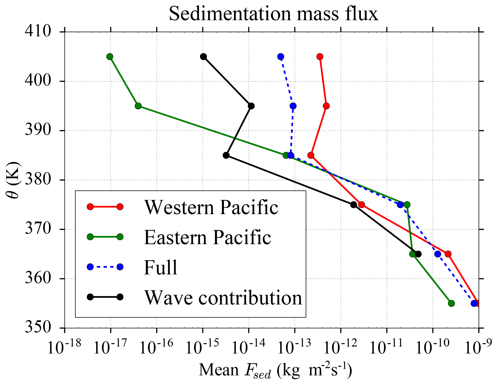
Figure 7Sedimentation water flux Fsed estimated from ATTREX observations in the eastern Pacific 2013 observations, western Pacific and for the whole campaign as a function of potential temperature. The wave stability impact is illustrated for the whole campaign by the black curve, which corresponds to the wave contribution to the flux . In the upper part of the TTL the wave stability impact reduces the sedimentation flux by about 10 % of the total flux.
4.1 An alternative mechanism to explain the clear-sky and cloudy-air relative humidity in the UTLS?
The frequency distribution of RHi in the upper troposphere shows two robust characteristics: (1) the common occurrence of 100 % relative humidity within clouds and (2) the high clear-sky supersaturations that get more frequent with increasing altitudes and decreasing temperatures in the TTL (Krämer et al., 2009). While those observations have both received explanations, the analysis presented above suggests that a new mechanism (wave-driven localization) may also contribute.
First, regarding (1), the explanation usually invoked is that the presence of ice crystals damps relative humidity variations towards saturation, by absorbing or releasing water molecules depending on the relative humidity. Using a theoretical parcel model framework, Korolev and Mazin (2003) explain this by the relaxation towards a quasi-equilibrium supersaturation state, close to RHi = 100 %. In their stochastic parcel model driven by colored noise temperature variability, Kärcher et al. (2014) also found a damping of the initial mean supersaturation by the ice crystals and a stabilization of the relative humidity with small fluctuations around 100 %. In both studies, large excursions away from RHi = 100 % were prevented by the stabilizing effect brought by the presence of the ice crystals.
In the simulations presented above (Fig. 6), the average relative humidity in clouds is also close to 100 %, but for a different reason. Indeed, contrary to the traditional explanations, the feedback of the cloud particles on the ambient relative humidity is not included in our simulations. Hence, ice crystals cannot regulate the vapor field towards RHi ≃ 100 %. What happens, on the contrary, is that only the ice crystals initially located near RHi ≃ 100 % remain and are constrained to follow the saturated regions due to the wave-driven localization.
Regarding point (2), it is thought that the increased occurrence of high supersaturations encountered in clear skies at low temperatures (Krämer et al., 2009) is due to the increase with decreasing temperature of the supersaturation threshold required for nucleation. These higher clear-sky supersaturations are often observed in the very cold TTL, and the absence of clouds in such conditions limits the efficiency of dehydration (Rollins et al., 2016). In our simulations (see for example Fig. 6), we also note that the amplitude of the RHi oscillations increases with altitude (whereas the temperature amplitude remains constant). The reason for these higher supersaturations at low temperatures in our simulations is the nonlinearity of the Clausius–Clapeyron relation with respect to temperature, combined with constant gravity wave temperature amplitude through the TTL. This may be seen from Eq. (21) (which is derived from the Clausius–Clapeyron equation): wave-induced RHi oscillations have their amplitude ΔRHi equal to
In our simulations, is the only factor that does depend on altitude (through the background state temperature gradient ). Given that increases with decreasing temperature (see Eq. 21) and the other factors are constant, it follows that high supersaturation (and subsaturation) are more common (and larger) at low temperatures.
Of course, our simplifications and the above considerations are not strictly applicable to the Earth cirrus clouds, which behave in a more complicated manner. For instance, in the TTL, clouds characterized by RHi ≃ 100 % generally have large numbers of ice crystals (Jensen et al., 2013; Rollins et al., 2016), which is consistent with the vapor-quenching explanation. Furthermore, even for TTL cirrus with low ice crystal number, the assumption made here of negligible water consumption is unrealistic. Damping of the super and subsaturation by the moving ice crystals will tend to broaden the equilibrium regions of RHi ≃ 100 %. Hence, we do not claim that the quenching does not occur and lead to RHi ≃ 100 %, but it is worthwhile to note that another mechanism can lead to the same relation. Our idealized examples may thus point to a process overlooked up to now.
4.2 Wave advection versus variability in sedimentation speed
The relevance of wave-driven localization to cirrus clouds' evolution and dehydration efficiency depends on their microphysical properties: size distribution and crystal shape. Those points are explained below.
First, regarding the size distribution, it is important to note that our considerations are relevant for crystals whose sedimentation speed vsed is close to , which limits the usefulness to rather small ice crystals (a few tens of microns for the maximum dimension). However, the sedimentation flux Fsed depends on the fourth- or fifth-order moment of the size distribution (Kärcher et al., 2014) and is hence more tied to the large ice crystals. The wave impact might hence be negligible if the crystals that dominate Fsed are large compared to those that are affected by the wave-driven localization. To investigate whether this is the case, we show in Fig. 8 the mean size distribution of the number, mass and mass flux of ice crystals from the ATTREX FCDP, and 2DS (2-D stereo probe) cloud probes during the 2014 field campaign. The mass and sedimentation flux are computed assuming spherical particles for the FCDP bins in which, for the 2DS, the maximum dimension, area and mass measured are directly used. The sedimentation speed needed for the mass-flux computation follows the work of Heymsfield and Westbrook (2010) with the measured maximum dimension, surface area and mass used as inputs to the formulas. Small ice crystals with sizes of a few tens of microns diameter or less dominate the number distribution, with a peak around 10 µm corresponding to fall speeds around a few millimeters per second. However, larger ice crystals become more important when the mass distribution is considered, and even more for the mass flux distribution. Nevertheless, the observations suggest that in the TTL, at levels higher than θ = 360 K, the mass flux is still dominated by crystals with maximum dimension smaller than 50 µm. In that case, the wave–sedimentation interaction described above will have an influence on the dehydration efficiency, since vsed is not much larger than .
Second, regarding crystal shape, we have been assuming so far that the ice crystals all have spherical shapes. Although this is mostly the case in observations of crystals dimensions below 65 µm at the largest, larger crystals are clearly aspherical (Lawson et al., 2008), which can strongly diminish their sedimentation speed (Jensen et al., 2008): for instance, the sedimentation speed for hexagonal plates might be diminished by 40 % relative to the spherical case (Jensen et al., 2008; Westbrook, 2008). This is especially important since those largest, aspherical ice crystals dominate Fsed. Hence, the sedimentation flux may be more affected by the microphysical characteristics of the crystals (their shape, etc.) than by the wave advection effect. Nevertheless, ATTREX observations do suggest that this effect is present. This might be related to the fact that, at high altitude, a large portion of the mass flux Fsed is associated with crystals below 65 µm maximum dimension (Fig. 7).
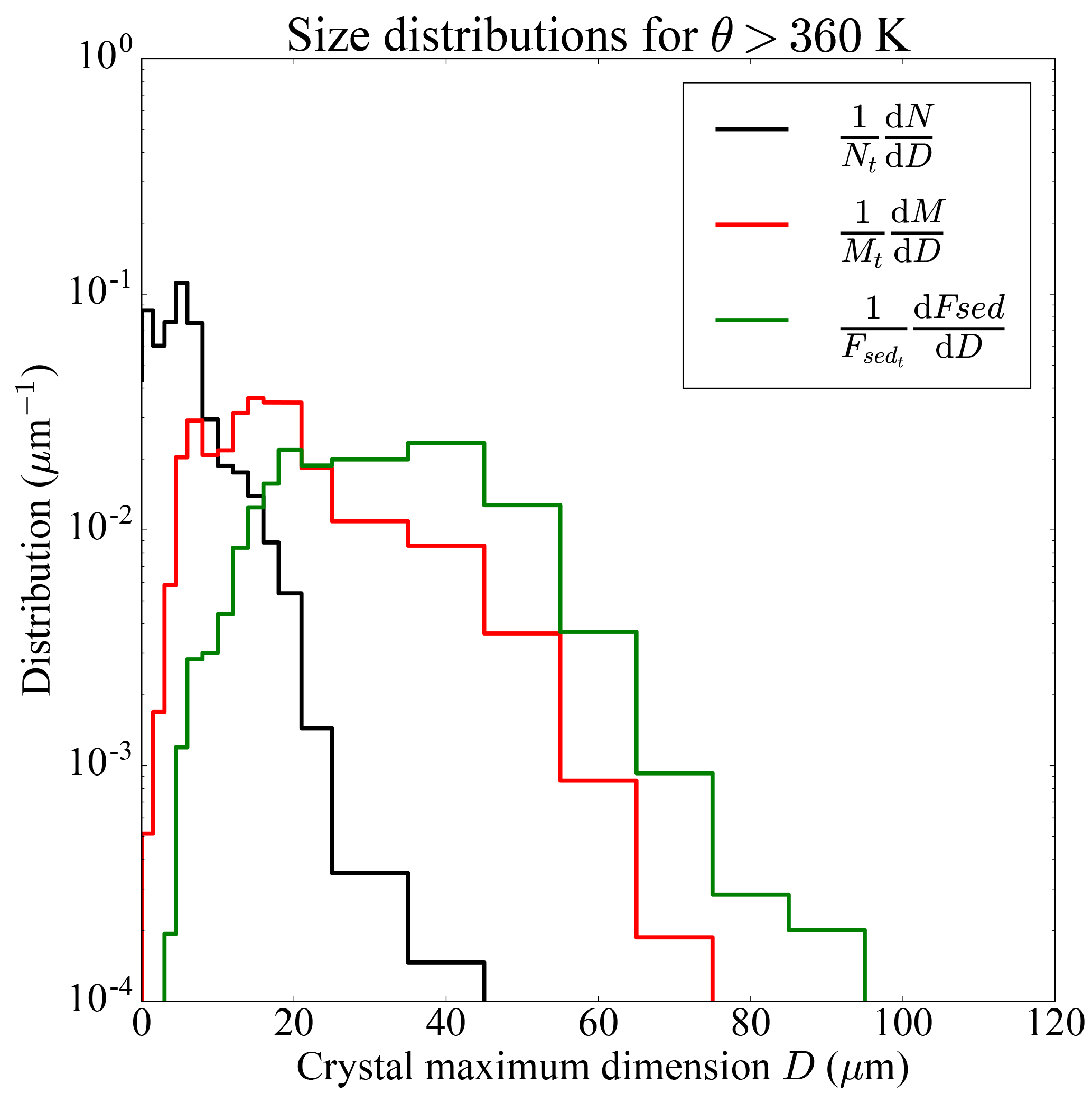
Figure 8Average ice crystal size distribution within cirrus clouds during ATTREX 2014 flights, above θ = 360 K. In black, number distribution; in red, mass distribution; in green, mass flux distribution. The distributions shown are composites of 2DS and FCDP measurements. The size considered is the maximum dimension, the diameter for spherical particles. It should be mentioned that the size retrieved by the FCDP is not strictly exact because the retrieval of size distribution from scattered light assumes spherical particles. The sedimentation speed needed for the mass flux computation are computed using the formula of Heymsfield and Westbrook (2010).
4.3 Representation in models
Our calculations emphasize the importance of an accurate representation of the waves for cirrus modeling. In particular, the simulations presented in Sect. 3.1 show that in the presence of the wave, ice crystals can survive in regions where the background environment is subsaturated. Climate models lack the vertical resolution to represent fine-vertical-scale equatorial waves, so that the processes described in this paper are in a large part absent. The situation is less critical for operational weather prediction models, but Podglajen et al. (2014) still found that large disagreements could arise between the winds represented in those products and the observed ones.
The role of equatorial and gravity waves has long been acknowledged in Lagrangian cirrus cloud models, which generally include a parameterization of wave fluctuations (Jensen and Pfister, 2004; Kärcher and Haag, 2004). Most of the time, however, only temperature fluctuations are accounted for, and the wave advection is ignored. The studies by Jensen et al. (2008) and by Grooß and Müller (2007) are exceptions, and the particle-following approach remains rarely used with most Lagrangian models only following air parcels. In models purely following air parcels (Fueglistaler and Baker, 2006; Spichtinger and Cziczo, 2010), a removal time is prescribed for the falling ice and the wave-driven localization is entirely absent. Column models in isentropic coordinates, such as the one of Jensen and Pfister (2004) and Ueyama et al. (2015), partly include this effect, but they neglect horizontal wind vertical shear which can modify the wave impact on the crystals'motion (see Sect. 3.1). By diminishing the average downward speed of the ice crystals, wave advection first limits the dehydration of the TTL, and then increases its average cloudiness by keeping surviving crystals within it. Neglecting that effect could add significant uncertainties in our understanding of the water budget of the TTL and lower stratosphere.
We have analytically investigated the impact of a monochromatic gravity wave on the motion of ice crystals. For an upward-propagating GW packet, assuming no water vapor release or depletion by the crystals, an interesting wave-driven localization effect is found, in which some of the ice crystals remain confined in a specific wave phase. This wave phase is characterized by positive vertical winds, which slow down the fall of the crystals.
The existence of the wave-driven localization is confirmed by idealized numerical simulations of ice crystals growth and/or sublimation and sedimentation under tropical tropopause conditions. We restricted ourselves to the case of a monochromatic large-scale wave, and did not consider ice nucleation or small-scale gravity waves, which should both be investigated by future work. Despite those limitations, our results provide a plausible and rather simple explanation for the relationship between waves and cirrus clouds observed in the tropical Pacific TTL by Kim et al. (2016). Indeed, in situ observations during ATTREX show that the cirrus clouds are associated with negative temperature anomalies in dry regions (over the tropical eastern Pacific) and with negative vertical temperature gradient anomalies in moister regions (over the tropical western Pacific). This observational finding is consistent with both our analytical results and our numerical simulations. Furthermore, from ATTREX observations, the wave-driven localization and wave wind advection might diminish the ice flux leaving the TTL by about 10 % relative to the flux estimated when the wave-induced vertical wind variations are ignored. This is due to the more frequent occurrence of positive vertical winds where the ice crystals are present.
Two main conclusions can be drawn from our study. First, there is a fundamental difference between air parcels and ice particles: due to wave-driven localization, waves can have an average impact on the motion of ice crystals even if they have none on air parcels'. Second, water vapor quenching by the ice is not the only mechanism to consider when examining the distribution of relative humidity in clouds. Ice crystals' motion in a variable relative humidity field is also highly relevant and should not be overlooked. Indeed, wave-driven localization guides ice crystals to concentrate where RHi ∼ 100 % without any effect of the ice crystals on the relative humidity.
Although we focused on TTL cirrus, the theory introduced here is general and might be relevant to other types of clouds or aerosols which are largely influenced by waves and the associated wind field. An example is the case of noctilucent clouds (NLCs) in the summer polar mesopause region. Rapp et al. (2002) have investigated the influence of waves on NLC and demonstrated that the interplay between sedimentation, transport by the wave vertical wind, and growth could lead to the NLC layer following the motion of the cold phase of the wave. However, if those authors also used particle trajectory calculations and emphasized the role of vertical wind in competition with sedimentation, they neglected the impact of the horizontal wind which can significantly modify the wave impact on sedimentation (see Sect. 3.1 and Appendix C). Another example of microphysical process strongly affected by waves is the case of polar stratospheric clouds, which are affected by mountain waves over the Antarctic Peninsula or the Scandinavian mountains (Carslaw et al., 1999) and could show similar relations to those presented here.
Besides the atmosphere, many other media, such as oceans and lakes, are perturbed by internal gravity waves. Those waves contribute to particle transport through the classical Stokes drift, mixing due to wave breaking and also through the resuspension of sediments due to the stress exerted by the induced flow on the bottom (Butman et al., 2006; Cacchione et al., 2002). Although it involves different physics, a parallel can be made between this last process and the irreversible wave-induced motion we describe: in both cases it is the combination of the wave presence and the particles' motion in relation to the flow that lead to irreversible transport by the wave. The effect of the waves on the sedimentation of particles (described in Sect. 2.1, before considering the growth and decay of ice crystals) might also directly play a role in sediment transport in oceans and lakes or particle transport in the atmosphere of any planet. Indeed, the theoretical derivation in Sect. 2.1 applies to any stratified fluids perturbed by internal waves and containing particles in suspension (that is, almost any stratified fluid).
Specifically for the atmosphere, a number of previous works have stressed the impact of waves on UTLS clouds. Here, we have unraveled yet another effect, which possibly provides an explanation for recently observed relations between waves and cirrus. Our results hence call for more quantitative observations of waves and cirrus clouds, in order to more precisely nail down the wave impact on clouds and improve its representation in models. Quasi-Lagrangian cloud and wave observations coupled with particle-following model simulations would be especially convenient to investigate this effect.
The ATTREX aircraft data used in this paper can be retrieved from NASA Earth Science Project Office (ESPO) at https://espoarchive.nasa.gov/archive/browse/attrex (Jensen et al., 2017).
To avoid strongly overestimating the effect of wave-driven vertical transport on sedimentation, it is important to recall that the wave amplitude is limited by a stability requirement. Shear and convective breaking of monochromatic gravity waves have been treated in a number of studies (Lindzen, 1981), and we adapt those considerations to our notations, to highlight where our two wave parameters ( and W) intervene.
We take the criterion that the Richardson number Ri must be larger than a critical value Ric. The Miles–Howard stability criterion suggests Ric ≃ , and a more conservative choice would be Ric ≃ 1. For simplicity and consistency with our configuration, we neglect the background shear; then the Richardson number induced by the monochromatic wave field is as follows:
with a = (a < 0 since we are interested in upward propagating waves).
Figure A1 represents the minimum Richardson number over all wave phases in our configuration. Examination of the figure or of Eq. (A1) shows that for , Ri ≥ 0.5. The condition Ri > is equivalent for the monochromatic upward propagating wave to the condition for convective stability, i.e., Ri > 0 or < 1. The condition Ri > 1 is a bit more restrictive and requires 0 ≥ a > ∼ −0.82. We will then restrict the chosen wave amplitude so that the minimum Ri remains above 1, i.e., < 0.82. Wave breaking and the generated turbulence probably has an important impact on vertical mixing and vertical transport of ice and water in the TTL (Podglajen et al., 2017), but this is not considered in our configuration, which focuses on propagating waves.
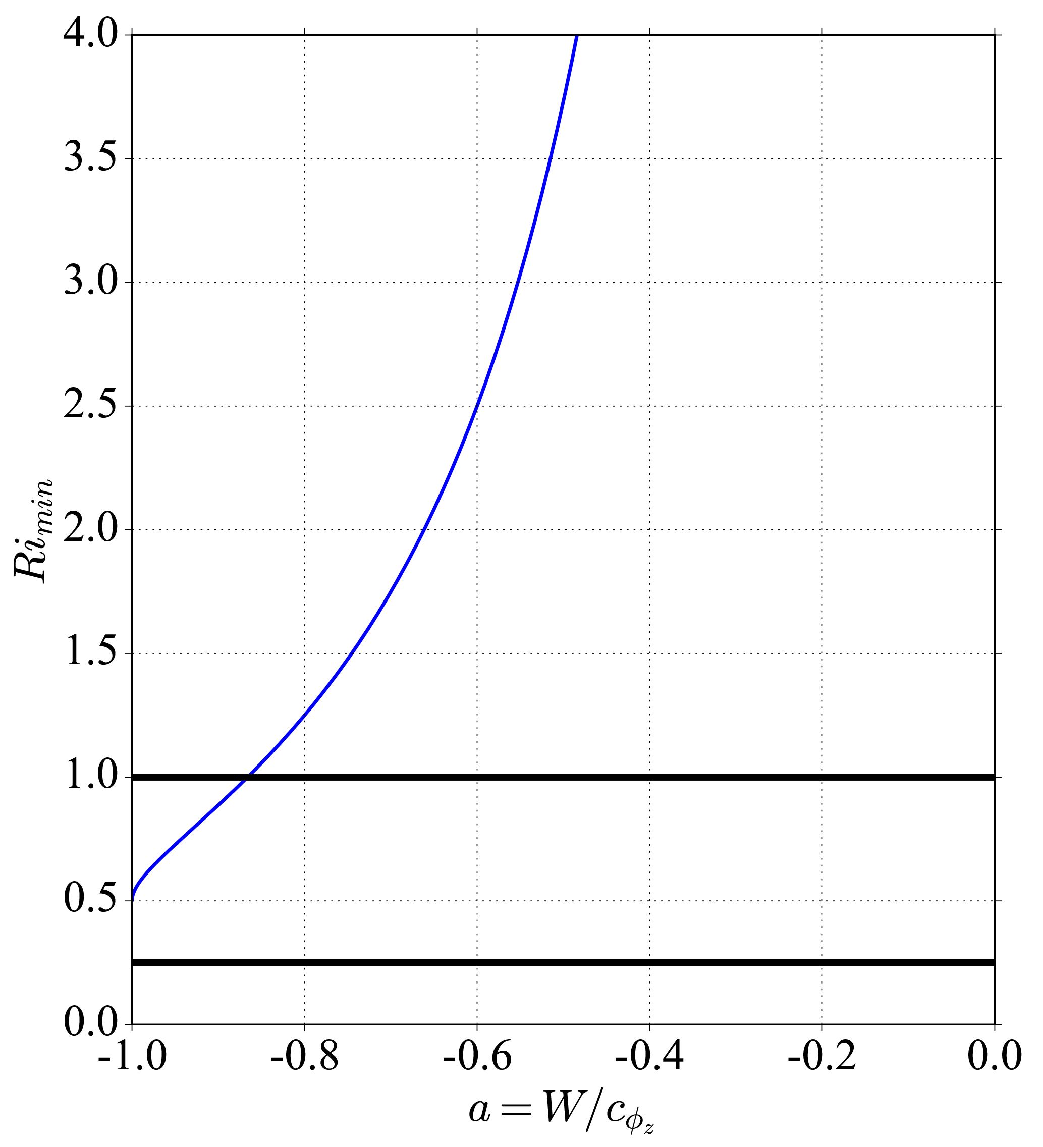
Figure A1Minimum Richardson number over all wave phases, as a function of the amplitude parameter .
Writing p = Ψ and q = r2, Eq. (23) reads as follows:
so that, with H(p, q) = − Ccos(p) + Dp, we have = and = . The system is therefore Hamiltonian, and the trajectories in the p–q space are given by the curves of constant H.
The existence of periodic orbits is equivalent to the existence of local extrema of the Hamiltonian function. Noting that the existence of fixed points (and extrema of H) for q > 0 requires that ω and m are of opposite signs, which implies that A and C are of the same sign. Given its expression, local extrema of H for q > 0 can then only be encountered for q = . Hence, there are local extrema of H iif there exists p ∈ [0; 2π] for which , ) = Csin(p) + D cancels and changes sign and for which , = C*cos(p) is of the sign of A (= ). It is easy to see that there exists such p iif < 1; since A and C are of the same sign; those extrema, which correspond to the elliptic points, are located where cos(p) > 0.
The expression of H enables us to determine the location of the separatrix which delimits the region of periodic orbits, when they exist. Noting pe (the phase of the elliptic point) and ps (that of the closest saddle point), and assuming A > 0, it can be seen from geometric arguments that the coordinates (p, q) of the separatrix are characterized by the following:
if H(ps, q = > H(pe, q = 0), otherwise by
The first case arises because q = r2 is physically required to be larger than 0. The general mathematical requirement for the separatrix (if negative q were possible) is the second case. Given those constraints, it is possible to find numerically the phase p = Ψsep of the intersections of the separatrix with the r = rf line, and hence the fraction ℱp of the phase space affected by that.
The theoretical analysis presented in this paper accounts for both the horizontal and the vertical wind components due to the wave. Figure C1 is similar to Fig. 6 but also shows the ice crystals' position when the horizontal wind induced by the wave is neglected. In the low RHi case (right panel of Fig. C1), contrasting the crystal positions between the full-wind and no-horizontal-wind simulations reveals a tendency of the remaining ice crystals to be present at higher altitude when full wave advection is accounted for. This difference between the full-wind and no-horizontal-wind simulations is even more striking for the high RHi scenario (left panel). Furthermore, when the horizontal wind is neglected, the proportion of ice crystals surviving after half a wave period is increased by a factor of 2 (moist case) to 3 (dry case). This shows the limits of the single-column approach.
It might seem surprising that, once the horizontal wind is neglected, the downward speed of the crystals at the elliptic point wc is similar whether or not the vertical wind is accounted for (see the orange and green dots in Fig. C1). This is due to the fact that when the vertical wind is taken into account but not the horizontal wind, the sedimentation speed at the elliptic fixed point is as follows:
so that the crystals have higher fall speeds and larger sizes than when neither the vertical nor the horizontal wind speeds are accounted for.
With only the wave vertical wind, the total vertical speed of the crystals wc is the sum of the vertical wind and the fall speed,
while with no wave wind the total vertical speed is just the crystal fall velocity:
Hence, interestingly, taking into account only the wave vertical wind increases the sedimenting ice flux at the elliptic point compared to the full-wind and no-wind cases, due to the increase in the size of the crystals when the vertical wind component is accounted for. This increase in the sedimenting mass flux occurs even so the positive vertical winds where the ice crystals are present would be expected to diminish that flux. However, one should recall that only the ice crystals confined near the elliptic point are concerned with this effect.

Figure C1Same as Fig. 6, but including ice crystal positions from simulations with the wave vertical wind accounted for but not the horizontal one (orange). As in Fig. 6, the blue dots are the ice crystals' positions for the full simulation (wave advection and temperature fluctuations), and the for the green dots both the horizontal and vertical winds induced by the wave have been neglected. The initial ice crystal radius used in both cases for all crystals is 5 µm.
This appendix compares the stability () within and outside of clouds in ATTREX observations, using cirrus cloud observations and vertical temperature profiles form the microwave temperature profiler. The results, consistent with those of Kim et al. (2016), complement them using the isentropic approach.
Figure D1 shows the mean lapse rate as a function of potential temperature, within and outside of clouds. In the upper TTL (above 380 K or about 16.5 km) over the western Pacific, the potential temperature lapse rate appears systematically lower within clouds compared to out of those, which is consistent with the results of Kim et al. (2016), who found anomalous negative lapse rate of wave temperature anomalies ddz within clouds. This difference between cloudy and cloud-free air is robust despite the limited number of independent events; it is seen in different flights in particular. It is also larger than the vertical change of stability in the upper TTL, so that it is not due to clouds being more prevalent in the lower part of the bins where stability is weaker.
This relationship between clouds and stability is further analyzed in Fig. D2, which presents the observed probability distribution of for cloudy air versus clear air, in the eastern and western Pacific and in different potential temperature ranges. In the eastern Pacific and in the western Pacific above 380 K, Fig. D2 shows a peak of the cloudy-air PDF (probability density function) in negative . The peak is shifted towards lower values of in the western Pacific above θ = 380 K than in the eastern Pacific, consistent with the results of Kim et al. (2016). Indeed, Kim et al. (2016) found that, in the western Pacific above 15 km, most clouds were characterized by negative ddz, whereas in the eastern Pacific clouds were seen both in positive and negative ddz. The picture provided by Fig. D2 is also consistent with the sensitivity to background moisture in the idealized and more realistic simulations results shown in Figs. 2 and 6: in the dry eastern Pacific, the ice crystals are more common in the minimum-temperature ddz ≃ 0 phase of the wave. In the moister western Pacific at high altitude, the ice crystals are focused in the ddz < 0 phase of the wave. In both cases, that phase is the phase where RHi ≃ 100 %.
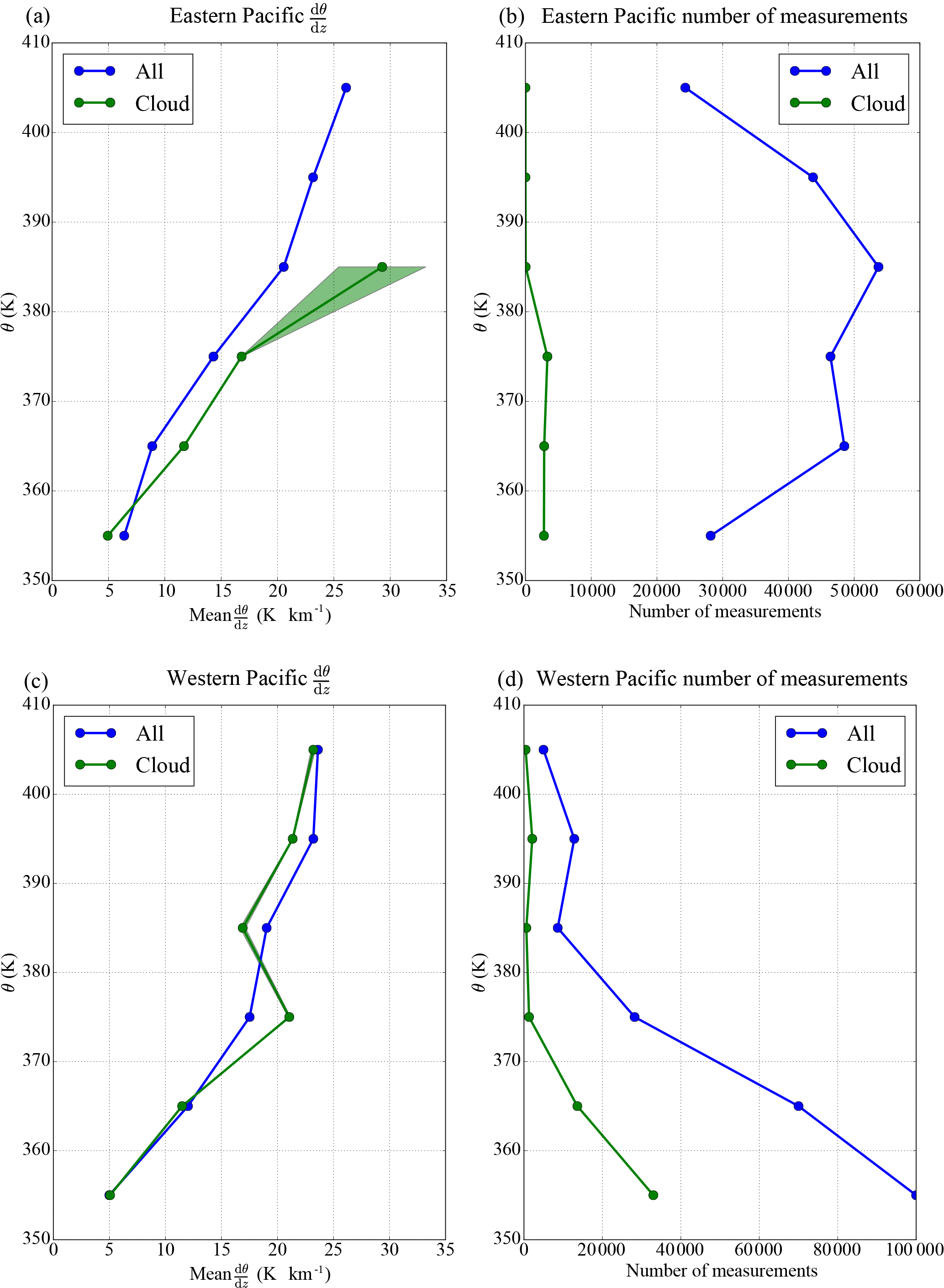
Figure D1(a, c) Average potential temperature vertical gradient in cloudy and cloud-free air in the eastern (a, b) and western Pacific (c, d). Panels (b, d) show the total and in cloud number of measurements as a function of altitude. In (a, c), the 1σ uncertainties are represented by shadings, but the amount of measurements are sufficient to make them indiscernible. This is nevertheless no statistical proof since the data come only from a few flights and are correlated.
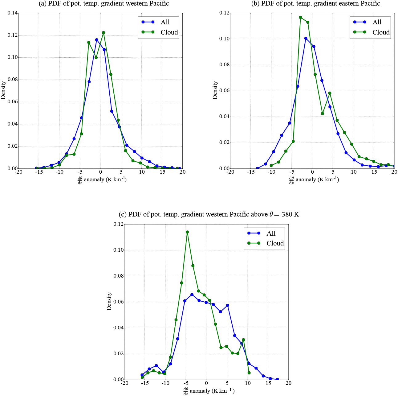
Figure D2Anomalies of stability distributions out of and within clouds from ATTREX observations in the (a) western Pacific, 2014, and (b) eastern Pacific, 2013. Panel (c) also corresponds to the western Pacific but only data above the potential temperature level 380 K.
AP and RP designed the study. AP performed the study, with suggestions from RP, AH and EJ. AP wrote the paper with contributions from all co-authors.
The authors declare that they have no conflict of interest.
The authors thank the teams involved in the development and exploitation of
the MMS, MTP, FCDP and 2DS instruments during the ATTREX campaign. Aurélien Podglajen thanks
Martina Krämer, Bernard Legras and Claudia Stubenrauch for their comments
on this work. We sincerely thank Peter Spichtinger and one anonymous referee for their
helpful comments and suggestions on the paper. Aurélien Podglajen,
Riwal Plougonven and Albert Hertzog
acknowledge support from the French ANR project StraDyVariUS (Stratospheric
Dynamic and Variability, ANR-13-BS06-0011-01) and from the French space
agency (CNES) through the Strateole 2 project.
Edited by: Peter Haynes
Reviewed by: Peter Spichtinger and one anonymous referee
Andrews, D., Holton, J., and Leovy, C.: Middle Atmosphere Dynamics, in: International geophysics series, Academic Press, San Diego, 1987. a
Boehm, M. T. and Verlinde, J.: Stratospheric influence on upper tropospheric tropical cirrus, Geophys. Res. Lett., 27, 3209–3212, https://doi.org/10.1029/2000GL011678, 2000. a
Butman, B., Alexander, P., Scotti, A., Beardsley, R., and Anderson, S.: Large internal waves in Massachusetts Bay transport sediments offshore, Cont. Shelf Res., 26, 2029–2049, https://doi.org/10.1016/j.csr.2006.07.022, 2006. a
Cacchione, D. A., Pratson, L. F., and Ogston, A. S.: The Shaping of Continental Slopes by Internal Tides, Science, 296, 724–727, https://doi.org/10.1126/science.1069803, 2002. a
Carslaw, K. S., Peter, T., Bacmeister, J. T., and Eckermann, S. D.: Widespread solid particle formation by mountain waves in the Arctic stratosphere, J. Geophys. Res.-Atmos., 104, 1827–1836, https://doi.org/10.1029/1998JD100033, 1999. a
Dinh, T., Fueglistaler, S., Durran, D., and Ackerman, T.: Cirrus and water vapour transport in the tropical tropopause layer – Part 2: Roles of ice nucleation and sedimentation, cloud dynamics, and moisture conditions, Atmos. Chem. Phys., 14, 12225–12236, https://doi.org/10.5194/acp-14-12225-2014, 2014. a
Dinh, T., Podglajen, A., Hertzog, A., Legras, B., and Plougonven, R.: Effect of gravity wave temperature fluctuations on homogeneous ice nucleation in the tropical tropopause layer, Atmos. Chem. Phys., 16, 35–46, https://doi.org/10.5194/acp-16-35-2016, 2016. a
Fritts, D. C. and Alexander, M. J.: Gravity wave dynamics and effects in the middle atmosphere, Rev. Geophys., 41, 1003, https://doi.org/10.1029/2001RG000106, 2003. a, b, c
Fueglistaler, S. and Baker, M. B.: A modelling study of the impact of cirrus clouds on the moisture budget of the upper troposphere, Atmos. Chem. Phys., 6, 1425–1434, https://doi.org/10.5194/acp-6-1425-2006, 2006. a
Grooß, J.-U. and Müller, R.: Simulation of ozone loss in Arctic winter 2004/2005, Geophys. Res. Lett., 34, l05804, https://doi.org/10.1029/2006GL028901, 2007. a
Heymsfield, A. J. and Westbrook, C. D.: Advances in the Estimation of Ice Particle Fall Speeds Using Laboratory and Field Measurements, J. Atmos. Sci., 67, 2469–2482, https://doi.org/10.1175/2010JAS3379.1, 2010. a, b, c
Hirsch, M., Smale, S., and Devaney, R.: Differential Equations, Dynamical Systems, and an Introduction to Chaos, Academic Press, Elsevier, Amsterdam, 2013. a
Jensen, E. and Pfister, L.: Transport and freeze-drying in the tropical tropopause layer, J. Geophys. Res.-Atmos., 109, D02207, https://doi.org/10.1029/2003JD004022, 2004. a, b
Jensen, E. J., Pfister, L., Bui, T. V., Lawson, P., Baker, B., Mo, Q., Baumgardner, D., Weinstock, E. M., Smith, J. B., Moyer, E. J., Hanisco, T. F., Sayres, D. S., Clair, J. M. S., Alexander, M. J., Toon, O. B., and Smith, J. A.: Formation of large (∼ 100 µm) ice crystals near the tropical tropopause, Atmos. Chem. Phys., 8, 1621–1633, https://doi.org/10.5194/acp-8-1621-2008, 2008. a, b, c
Jensen, E. J., Pfister, L., Bui, T.-P., Lawson, P., and Baumgardner, D.: Ice nucleation and cloud microphysical properties in tropical tropopause layer cirrus, Atmos. Chem. Phys., 10, 1369–1384, https://doi.org/10.5194/acp-10-1369-2010, 2010. a
Jensen, E. J., Diskin, G., Lawson, R. P., Lance, S., Bui, T. P., Hlavka, D., McGill, M., Pfister, L., Toon, O. B., and Gao, R.: Ice nucleation and dehydration in the Tropical Tropopause Layer, P. Natl. Acad. Sci. USA, 110, 2041–2046, https://doi.org/10.1073/pnas.1217104110, 2013. a, b
Jensen, E. J., Ueyama, R., Pfister, L., Bui, T. V., Alexander, M. J., Podglajen, A., Hertzog, A., Woods, S., Lawson, R. P., Kim, J.-E., and Schoeberl, M. R.: High-frequency gravity waves and homogeneous ice nucleation in tropical tropopause layer cirrus, Geophys. Res. Lett., 43, 6629–6635, https://doi.org/10.1002/2016GL069426, 2016. a
Jensen, E. J., Pfister, L., Jordan, D. E., Bui, T. V., Ueyama, R., Singh, H. B., Thornberry, T. D., Rollins, A. W., Gao, R., Fahey, D. W., Rosenlof, K. H., Elkins, J. W., Diskin, G. S., DiGangi, J. P., Lawson, R. P., Woods, S., Atlas, E. L., Navarro Rodriguez, M. A., Wofsy, S. C., Pittman, J., Bardeen, C. G., Toon, O. B., Kindel, B. C., Newman, P. A., McGill, M. J., Hlavka, D. L., Lait, L. R., Schoeberl, M. R., Bergman, J. W., Selkirk, H. B., Alexander, M. J., Kim, J., Lim, B. H., Stutz, J., and Pfeilsticker, K.: The NASA Airborne Tropical Tropopause Experiment: High-Altitude Aircraft Measurements in the Tropical Western Pacific, B. Am. Meteorol. Soc., 98, 129–143, https://doi.org/10.1175/BAMS-D-14-00263.1, 2017. a
Kärcher, B. and Haag, W.: Factors controlling upper tropospheric relative humidity, Ann. Geophys., 22, 705–715, https://doi.org/10.5194/angeo-22-705-2004, 2004. a
Kärcher, B. and Lohmann, U.: A parameterization of cirrus cloud formation: Homogeneous freezing of supercooled aerosols, J. Geophys. Res., 107, 4010, https://doi.org/10.1029/2001JD000470, 2002. a
Kärcher, B., Dörnback, A., and Sölch, I.: Supersaturation Variability and Cirrus Ice Crystal Size Distributions, J. Atmos. Sci., 71, 2905–2926, https://doi.org/10.1175/JAS-D-13-0404.1, 2014. a, b
Kay, J. E. and Wood, R.: Timescale analysis of aerosol sensitivity during homogeneous freezing and implications for upper tropospheric water vapor budgets, Geophys. Res. Lett., 35, L10809, https://doi.org/10.1029/2007GL032628, 2008. a
Kim, J.-E.: Impacts of Atmospheric Waves on Tropical Convection and the Tropical Tropopause Layer, PhD thesis, University of Colorado, Colorado, http://scholar.colorado.edu/atoc_gradetds/53 (last access: 20 July 2018), 2015. a
Kim, J.-E. and Alexander, M. J.: A new wave scheme for trajectory simulations of stratospheric water vapor, Geophys. Res. Lett., 40, 5286–5290, https://doi.org/10.1002/grl.50963, 2013. a
Kim, J.-E. and Alexander, M. J.: Direct impacts of waves on tropical cold point tropopause temperature, Geophys. Res. Lett., 42, 1584–1592, https://doi.org/10.1002/2014GL062737, 2015. a
Kim, J.-E., Alexander, M. J., Bui, T. P., Dean-Day, J. M., Lawson, R. P., Woods, S., Hlavka, D., Pfister, L., and Jensen, E. J.: Ubiquitous influence of waves on tropical high cirrus clouds, Geophys. Res. Lett., 43, 5895–5901, https://doi.org/10.1002/2016GL069293, 2016. a, b, c, d, e, f, g, h, i, j, k, l
Korolev, A. and Mazin, I.: Supersaturation of Water Vapor in Clouds, J. Atmos. Sci., 60, 2957–2974, https://doi.org/10.1175/1520-0469(2003)060<2957:SOWVIC>2.0.CO;2, 2003. a
Krämer, M., Schiller, C., Afchine, A., Bauer, R., Gensch, I., Mangold, A., Schlicht, S., Spelten, N., Sitnikov, N., Borrmann, S., de Reus, M., and Spichtinger, P.: Ice supersaturations and cirrus cloud crystal numbers, Atmos. Chem. Phys., 9, 3505–3522, https://doi.org/10.5194/acp-9-3505-2009, 2009. a, b, c, d
Lawson, R. P., Pilson, B., Baker, B., Mo, Q., Jensen, E., Pfister, L., and Bui, P.: Aircraft measurements of microphysical properties of subvisible cirrus in the tropical tropopause layer, Atmos. Chem. Phys., 8, 1609–1620, https://doi.org/10.5194/acp-8-1609-2008, 2008. a, b, c
Lindzen, R. S.: Turbulence and stress owing to gravity wave and tidal breakdown, J. Geophys. Res.-Oceans, 86, 9707–9714, https://doi.org/10.1029/JC086iC10p09707, 1981. a
Luo, B. P., Peter, T., Fueglistaler, S., Wernli, H., Wirth, M., Kiemle, C., Flentje, H., Yushkov, V. A., Khattatov, V., Rudakov, V., Thomas, A., Borrmann, S., Toci, G., Mazzinghi, P., Beuermann, J., Schiller, C., Cairo, F., Di Donfrancesco, G., Adriani, A., Volk, C. M., Strom, J., Noone, K., Mitev, V., MacKenzie, R. A., Carslaw, K. S., Trautmann, T., Santacesaria V., and Stefanutti, L.: Dehydration potential of ultrathin clouds at the tropical tropopause, Geophys. Res. Lett., 30, 1557–1560, 2003. a, b, c
Magee, N., Moyle, A. M., and Lamb, D.: Experimental determination of the deposition coefficient of small cirrus-like ice crystals near −50 Celsius, Geophys. Res. Lett., 33, L17813, https://doi.org/10.1029/2006GL026665, 2006. a
McFarquhar, G. M., Heymsfield, A. J., Spinhirne, J., and Hart, B.: Thin and subvisual tropopause tropical cirrus: Observations and radiative impacts, J. Atmos. Sci., 57, 1841–1853, https://doi.org/10.1175/1520-0469(2000)057<1841:TASTTC>2.0.CO;2, 2000. a
Mitchell, D. L.: Use of Mass- and Area-Dimensional Power Laws for Determining Precipitation Particle Terminal Velocities, J. Atmos. Sci., 53, 1710–1723, https://doi.org/10.1175/1520-0469(1996)053<1710:UOMAAD>2.0.CO;2, 1996. a
Peter, T., Luo, B. P., Wirth, M., Kiemle, C., Flentje, H., Yushkov, V. A., Khattatov, V., Rudakov, V., Thomas, A., Borrmann, S., Toci, G., Mazzinghi, P., Beuermann, J., Schiller, C., Cairo, F., Di Donfrancesco, G., Adriani, A., Volk, C. M., Strom, J., Noone, K., Mitev, V., MacKenzie, R. A., Carslaw, K. S., Trautmann, T., Santacesaria, V., and Stefanutti, L.: Ultrathin tropical tropopause clouds (UTTCs): I. Cloud morphology and occurrence, Atmos. Chem. Phys., 3, 1083–1091, https://doi.org/10.5194/acp-3-1083-2003, 2003. a
Podglajen, A., Hertzog, A., Plougonven, R., and Žagar, N.: Assessment of the accuracy of (re)analyses in the equatorial lower stratosphere, J. Geophys. Res., 119, 11166–11188, https://doi.org/10.1002/2014JD021849, 2014. a
Podglajen, A., Hertzog, A., Plougonven, R., and Legras, B.: Lagrangian temperature and vertical velocity fluctuations due to gravity waves in the lower stratosphere, Geophys. Res. Lett., 43, 3543–3553, https://doi.org/10.1002/2016GL068148, 2016a. a, b
Podglajen, A., Plougonven, R., Hertzog, A., and Legras, B.: A modelling case study of a large-scale cirrus in the tropical tropopause layer, Atmos. Chem. Phys., 16, 3881–3902, https://doi.org/10.5194/acp-16-3881-2016, 2016b. a
Podglajen, A., Bui, T. P., Dean-Day, J. M., Pfister, L., Jensen, E. J., Alexander, M. J., Hertzog, A., Kärcher, B., Plougonven, R., and Randel, W. J.: Small-scale wind fluctuations in the tropical tropopause layer from aircraft measurements: occurrence, nature and impact on vertical mixing, J. Atmos. Sci., 74, 3847–3869, https://doi.org/10.1175/JAS-D-17-0010.1, 2017. a, b, c
Potter, B. E. and Holton, J. R.: The Role of Monsoon Convection in the Dehydration of the Lower Tropical Stratosphere, J. Atmos. Sci., 52, 1034–1050, https://doi.org/10.1175/1520-0469(1995)052<1034:TROMCI>2.0.CO;2, 1995. a
Pruppacher, H. R. and Klett, J. D.: Microphysics of clouds and precipitation, D. Reidel Publishing Company, Dordrecht, Holland, 1978. a, b, c, d
Rapp, M., Lübken, F. J., Müllemann, A., Thomas, G. E., and Jensen, E. J.: Small-scale temperature variations in the vicinity of NLC: Experimental and model results, J. Geophys. Res.-Atmos., 107, AAC 11-1–AAC 11-20, https://doi.org/10.1029/2001JD001241, 2002. a, b
Rollins, A. W., Thornberry, T. D., Gao, R. S., Woods, S., Lawson, R. P., Bui, T. P., Jensen, E. J., and Fahey, D. W.: Observational constraints on the efficiency of dehydration mechanisms in the tropical tropopause layer, Geophys. Res. Lett., 43, 2912–2918, https://doi.org/10.1002/2016GL067972, 2016. a, b
Skrotzki, J., Connolly, P., Schnaiter, M., Saathoff, H., Möhler, O., Wagner, R., Niemand, M., Ebert, V., and Leisner, T.: The accommodation coefficient of water molecules on ice – cirrus cloud studies at the AIDA simulation chamber, Atmos. Chem. Phys., 13, 4451–4466, https://doi.org/10.5194/acp-13-4451-2013, 2013. a, b
Spichtinger, P. and Cziczo, D. J.: Impact of heterogeneous ice nuclei on homogeneous freezing events in cirrus clouds, J. Geophys. Res.-Atmos., 115, D14208, https://doi.org/10.1029/2009JD012168, 2010. a
Spichtinger, P. and Krämer, M.: Tropical tropopause ice clouds: a dynamic approach to the mystery of low crystal numbers, Atmos. Chem. Phys., 13, 9801–9818, https://doi.org/10.5194/acp-13-9801-2013, 2013. a
Ueyama, R., Jensen, E. J., Pfister, L., and Kim, J.-E.: Dynamical, convective, and microphysical control on wintertime distributions of water vapor and clouds in the tropical tropopause layer, J. Geophys. Res.-Atmos., 120, 10483–10500, https://doi.org/10.1002/2015JD023318, 2015. a
Wallace, J. and Kousky, V. E.: Observational Evidence of Kelvin Waves in the Tropical Stratosphere, J. Atmos. Sci., 25, 900–907, https://doi.org/10.1175/1520-0469(1968)025<0900:OEOKWI>2.0.CO;2, 1968. a
Westbrook, C. D.: The fall speeds of sub-100 µm ice crystals, Q. J. Roy. Meteorol. Soc., 134, 1243–1251, https://doi.org/10.1002/qj.290, 2008. a
- Abstract
- Introduction
- Theory
- Wave advection impact in realistic settings and in observations
- Discussion
- Conclusions
- Data availability
- Appendix A: Note on wave stability
- Appendix B: Hamiltonian structure of the equations
- Appendix C: Impact of neglecting the horizontal wind induced by the wave
- Appendix D: Clouds and stability during ATTREX
- Author contributions
- Competing interests
- Acknowledgements
- References